OzDES multi-fibre spectroscopy for the Dark Energy Survey: first-year operation and results

Abstract

OzDES is a five-year, 100-night, spectroscopic survey on the Anglo-Australian Telescope, whose primary aim is to measure redshifts of approximately 2,500 Type Ia supernovae host galaxies over the redshift range $0.1<z<1.2$, and derive reverberation-mapped black hole masses for approximately 500 active galactic nuclei and quasars over $0.3<z<4.5$. This treasure trove of data forms a major part of the spectroscopic follow-up for the Dark Energy Survey for which we are also targeting cluster galaxies, radio galaxies, strong lenses, and unidentified transients, as well as measuring luminous red galaxies and emission line galaxies to help calibrate photometric redshifts.

Here we present an overview of the OzDES program and our first-year results. Between Dec 2012 and Dec 2013, we observed over 10,000 objects and measured more than 6,000 redshifts. Our strategy of retargeting faint objects across many observing runs has allowed us to measure redshifts for galaxies as faint as $m_{r}=25$ mag. We outline our target selection and observing strategy, quantify the redshift success rate for different types of targets, and discuss the implications for our main science goals. Finally, we highlight a few interesting objects as examples of the fortuitous yet not totally unexpected discoveries that can come from such a large spectroscopic survey.

1 INTRODUCTION

The Australian Dark Energy Survey (OzDES) has been designed to provide efficient spectroscopic follow-up of targets identified from imaging by the Dark Energy Survey (DES; Flaugher, 2005; Diehl et al., 2014). OzDES extends DES by enabling new science goals that cannot be achieved without spectroscopic information — such as supernova cosmology and reverberation mapping of active galactic nuclei (AGN). We also enhance DES by providing an important source of calibration data for photometric redshifts, which are the cornerstone for the majority of the DES science programs.

The 3.9m Anglo-Australian Telescope (AAT) used by OzDES and the CTIO 4m Blanco telescope used by DES are ideal partners for spectroscopy and imaging because they have well matched $\sim$2 degree diameter fields of view (see Fig. 1). The AAT and CTIO 4m are similar in several respects — both are 4m class telescopes that were commissioned in 1974 and both have recently been rejuvenated with powerful new instrumentation: in the case of CTIO it is the 570 mega-pixel Dark Energy Camera (DECam; Diehl et al., 2012; Flaugher et al., 2012), while on the AAT it is the new efficient AAOmega spectrograph (Smith et al., 2004) coupled with the Two Degree Field (2dF) 400-fibre multi-object fibre-positioning system (Lewis et al., 2002).

The DES program consists of a wide-field survey covering 5000 square degrees, as well as a rolling survey of ten fields that cover a total of 30 square degrees (Diehl et al., 2014). These ten fields (see Table 1 for the sky coordinates) are targeted repeatedly over the course of the survey with a cadence of approximately 6 days in order to find transient objects, such as supernovae, and monitor variable objects, such as AGN. OzDES repeatedly targets these ten fields, selecting objects that range in brightness from $m_{r}\sim 17$ to $m_{r}\sim 25$ mag, a range of more than a thousand in flux density. Once a redshift is obtained, we deselect the target (with some exceptions). Objects that lack a redshift are observed until a redshift is measured. This tactic allows us to obtain redshifts for targets far fainter than ever previously achieved with the AAT. Together this means we can run an efficient survey of bright objects while simultaneously acquiring spectra for much fainter objects.

Table 1: Center coordinates of the ten DES SN fields.

Field Name	R.A. (h m s)	Decl. ($\circ$ ′ ′′)	Comment*
E1	00 31 29.9	-43 00 35	ELAIS$\dagger$ S1
E2	00 38 00.0	-43 59 53
S1	02 51 16.8	00 00 00	Stripe 82$\ddagger$
S2	02 44 46.7	-00 59 18
C1	03 37 05.8	-27 06 42	CDFS$\S$
C2	03 37 05.8	-29 05 18
C3 (deep)	03 30 35.6	-28 06 00
X1	02 17 54.2	-04 55 46	XMM-LSS$\parallel$
X2	02 22 39.5	-06 24 44
X3 (deep)	02 25 48.0	-04 36 00
*Overlap with areas covered by other surveys.
$\dagger$European Large-Area ISO Survey.
$\ddagger$An equatorial region repeatedly imaged by SDSS.
$\S$Chandra Deep Field South survey.
$\parallel$X-ray Multi Mirror Large Scale Structure survey.

OzDES has a total of 100 nights distributed across five years during the DES observing seasons (August to January). The first season of OzDES began in 2013B (August 2013 to January 2014) with 12 nights (designated as Y1). Allocations will progressively increase each year, to accommodate the increasing number of supernovae host galaxies that DES will have accumulated in subsequent years.

In the 2012B (August 2012 to January 2013) semester, a year before the start of DES and OzDES, the DECam was used to execute the DES SN program as part of its Science Verification (SV) phase of commissioning. In parallel, AAT/AAOmega-2dF time was awarded for the observation of the DES SN fields in a precursor program to OzDES. Supplementary observing time (1 night during SV and 2 nights during Y1) was also obtained through the National Optical Astronomy Observatory (NOAO).

In this paper, we present an overview of OzDES and the results obtained during the SV and Y1 seasons. Non-DES fields and targets observed in the SV season are excluded from the analysis. When appropriate, we also discuss changes and improvements to the OzDES in Y2 (2014B, August 2014 to January 2015).

We organise the paper as follows: In $\S$ 2 we summarise our science goals and in $\S$ 3 we present the operational details that were current at the end of Y1, highlighting what was modified to improve the efficiency of the survey for Y2. Results of redshifts and quality assessments are presented in $\S$ 4, followed by discussions of implications for science in $\S$ 5. Finally, we conclude in $\S$ 6.

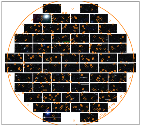
Figure 1: The 2dF spectrograph has 392 optical fibres to be placed at positions across a field of view 2.1 degree in diameter (large orange circle). This is well matched to the DECam field of view (image mosaic in the background), making spectroscopic follow-up very efficient. The small orange circles represent the locations of targets selected for one set of AAT observations.

2 Science Goals

Here we outline the wide range of science goals we aim to achieve with OzDES. Each science goal may require one or more types of target and the targeting strategies evolve with time. Details of the target types used in SV and Y1 are described in $\S$ 3.3.

2.1 Type Ia Supernova Cosmology

The main science motivation of OzDES is to obtain host galaxy spectroscopic redshifts for a sample of 2,500 Type Ia SNe discovered by DES, with the goal of improving measurements of the Universe’s global expansion history. This goal is efficiently achieved with AAT’s unique combination of multi-object fibre-fed spectroscopy and wide field of view.

Spectroscopy of live supernovae within a few weeks of maximum light serves the dual purpose of typing the transient (determining whether it is a Type Ia SN) and measuring its redshift. However, the spatial density of SNe Ia that are bright enough to be observed with the AAT at any instant in time is only a handful per square degree. An 8–10 metre class telescope is often required for such observations, but can usually only observe one object at a time. This mode of follow-up is thus time-consuming and requires an unrealistically large quantity of resources to acquire a large sample.

Alternatively, well sampled multicolour light curves can be used to reliably identify a SN Ia (Sako et al., 2011), after which a spectrum of the host galaxy can be used to measure its precise redshift. Host galaxy redshifts can also be used to improve photometric classification (Olmstead et al., 2014).

Host galaxies can be observed at any time, even after the supernova has faded. Thus one can wait to collect many supernovae in a field before measuring their host-galaxy redshifts efficiently with multi-object spectroscopy. This strategy has been tested in the Sloan Digital Sky Survey (SDSS-II, Olmstead et al., 2014) and the SuperNova Legacy Survey (SNLS, Lidman et al., 2013).

2.2 AGN Reverberation Mapping

The other primary science goal of OzDES is reverberation mapping of AGN and quasars. Reverberation mapping (Blandford & McKee, 1982; Peterson, 1993) is an effective way to measure supermassive black hole masses in AGN, over much of the age of the universe. This is possible because the continuum emission from the AGN accretion disk is variable, and this continuum emission photoionizes the clouds of gas at larger scales that give rise to the characteristic broad emission lines of most AGN. As the continuum emission varies in intensity, the broad emission lines reverberate in response with a time delay that depends on the light travel time from the continuum source.

Measurement of this time delay provides a geometric size for the broad line region. This size scale can be used to measure the mass of the supermassive black hole through application of the virial theorem and measurement of the velocity width of the broad emission line. Approximately 50 AGN have reverberation-based black hole masses to date, and the masses of these black holes agree well with mass measurements from stellar dynamics (Davies et al., 2006; Onken et al., 2014) and yield the same slope as the $M-\sigma_{*}$ relation that holds for quiescent galaxies (Woo et al., 2010; Grier et al., 2013). The size scale, typically determined from the H$\beta$ emission line, is also very well correlated with the AGN luminosity with the $R\propto L^{1/2}$ scaling expected from a simple photoionization model (e.g. Bentz et al., 2013). The relatively small scatter in this relation was used by Watson et al. (2011) to demonstrate that AGN could be used as standard candles.

The current sample of about 50 AGN with reverberation-based masses are all in low to moderate luminosity AGN, and nearly all in the relatively nearby universe ($z<0.3$). This is because reverberation mapping requires a substantial amount of telescope time to measure the time lags, and it has proven most straightforward to get the necessary allocation to observe bright objects with small telescopes. The lower-luminosity AGN also have lags of only days to weeks, and thus can be measured with a single semester of data. It is much more difficult to measure the year or longer lags of the most luminous AGN at redshifts $z>1$ and higher (although see Kaspi et al., 2007); yet these AGN are arguably the most interesting as they represent the majority of supermassive black hole growth in the universe. OzDES is presently monitoring $\sim$1000 AGN up to $z\approx 4$ and aims to measure reverberation lags and black hole masses for approximately 40% of the final sample (King et al., in prep). This new, multi-object reverberation mapping project, as well as other similar efforts (Shen et al., 2015), will provide a wealth of new data on black hole masses out to and beyond the peak of the AGN era. We will also use new measurements of the radius-luminosity relation to construct a Hubble diagram out to higher redshifts than can be reached with supernovae, which provides some complementary constraints on the time variation in dark energy (King et al., 2014).

2.3 Transients

Concurrent OzDES and DES observing enables time-critical spectroscopic observations of transients discovered in imaging. With a monthly observing cadence, OzDES is expected to target several hundred active transients, putting these at highest priority. This sample, supplemented by observations of fainter events by larger telescopes, will provide crucial validation of the photometric SN classification and enable detailed studies of these SNe.

We target all kinds of transient candidates, including those with uncertain physical nature. A survey of this size and scope expects to find surprises in the data. With our targeting strategy we aim to investigate the unexpected and potentially find as-yet unidentified classes of transients.

2.4 Photo-$z$ training

A core requirement of DES is to obtain accurate photometric redshifts (photo-$z$) for the majority of galaxies in the wide survey. This will enable key science goals, such as the measurement of baryon acoustic oscillations (BAO) with millions of galaxies, and the use of weak lensing for cosmology. Our spectra play an important role in providing a spectroscopic sample for calibrating and testing the DES photometric redshifts, and a significant number of our fibres are allocated to Luminous Red Galaxies (LRG), Emission Line Galaxies (ELG), and other photo-$z$ targets.

Redshifts from OzDES have already been used in a number of recently published studies on DES photometric redshifts. Sánchez et al. (2014) have used the redshifts to evaluate the performance of various photo-$z$ methods on DES SV data and found several codes to produce photo-$z$ precisions and outlier fractions that satisfy DES science requirements. Banerji et al. (2015) combines optical data from DES and near-infrared (NIR) data from VISTA Hemisphere Survey (VHS; McMahon et al., 2013) to improve photo-$z$ performance. In particular, selection criteria based on optical-NIR colors are applied to identify LRG targets at high redshift ($z\mathrel{\hbox{\hbox to0.0pt{\hbox{\lower 3.0pt\hbox{$\sim$}}\hss}\hbox{\raise 1.0pt\hbox{$>$}}}}0.5$) for OzDES. Spectroscopic results are used to verify the effectiveness of this selection method.

2.5 Radio galaxies, cluster galaxies, and strong lenses

The large number of fibres available to 2dF allows us to pursue a wide range of supplementary science goals. These include the following:

• Gathering redshifts of galaxies selected from the ATLAS (Australia Telescope Large Area Survey; Norris et al., 2006, Franzen et al. in prep, Banfield et al. in prep). ATLAS is a deep, 14/17 uJy/beam rms, 1.4 GHz survey of 3.6/2.7 deg² of the CDFS/ELAIS-S1 survey fields which have >90% overlap with the DES deep imaging. ATLAS is being used to study the astrophysics of radio sources, and is also being used as a pathfinder to develop the science and techniques for the primary radio continuum survey (EMU; Norris et al., 2011) of the Australian Square Kilometre Array Pathfinder (ASKAP). ATLAS has detected over 5000 radio sources of which at least half will be targeted by OzDES over the course of the survey. These redshifts will be used to determine the evolution of the faint radio population, including both star forming galaxies and radio AGN, up to redshift greater than one. They will also be used to calibrate photometric and statistical redshift algorithms for use with the 70 million EMU sources (for which spectroscopy is impractical). Furthermore, the detected optical emission lines will provide insights into the detailed astrophysics within these galaxies, including distinguishing star forming galaxies from AGN.

• Confirming previously unknown cluster candidates and gathering redshifts for cluster galaxies, especially central galaxies for the calibration of the cluster red sequence, as well as validation of cluster photometric redshifts. Our repeated returns to the same field allow us to collect redshifts for multiple galaxies in a single cluster. Usually this is impossible for all but very nearby clusters because the instrumental limit of fibre collisions prevents one from measuring closely neighbouring galaxies in the same exposure.

• Measuring redshifts for both the lens and the background lensed galaxy or quasar in strong lens candidates. Some of the lensed quasar targets may be suitable for time-delay experiments.

2.6 Calibration

About 10% of fibres are used for targets that facilitate the the calibration of the data. These include:

• Regions that are free of objects (sky fibres). Some of our targets are 100 times or more fainter than the sky in the $2{\hbox{${}^{\prime\prime}$}}$ fibre aperture, so a good estimate of the sky brightness is crucial.

• F stars that are used to monitor throughput, which is heavily dependent on the seeing and the amount of cloud cover. Up to 15 F stars are observed per field and used to derive a mean sensitivity curve. The variation of the sensitivity curve over each plate allows for an estimate of the accuracy of the flux calibration and the mean value allows us to appropriately weight data that are obtained over multiple occasions.

• Candidate hot (T${}_{\rm eff}\sim 20,000~{}\rm{K}$) DA (hydrogen atmosphere) white dwarfs (WDs) that can be used as primary flux calibrators for the DES deep fields. Stellar atmosphere modeling uncertainties for hot DA WDs are small so that synthetic photometry can be compared with DES observations with an expected accuracy of 2–3% or better per candidate. A collection of $\sim$100 such candidates over the DES deep fields will allow one to test the accuracy of the photometric calibration of the DES deep fields. The number of known DA WDs in the DES deep fields is currently too small to make this test, so we aim to find new ones.

3 Observing Strategy

3.1 Instrument Setup and Observations

The 2dF robotic positioner allows up to 392 targets to be observed simultaneously over a field of view 2.1 degrees in diameter (there are also 8 fibre bundles for guiding). The projected fibre diameter is approximately two arcsec. Two sets of fibres are provided on separate field plates mounted back-to-back on a tumbler. Configuration of all fibres on a single plate takes about 40 minutes and can be done as the other plate is being observed, thereby greatly reducing overheads. A minimum separation of 30 to 40 arcsec between fibres is imposed by the physical size of the rectangular fibre buttons. This constraint and other hardware limits are respected by the custom fibre configuration software.

The fibres feed AAOmega, which is a bench mounted double beam spectrograph sitting in one of the Coude rooms of the AAT. The light from the fibres is first collimated with a mirror before passing through a dichroic which splits the light at 570 nm into two arms, one red and one blue. In the blue arm, we used the 580V grating (dispersion of 1 A per pixel). In the red arm, we used the 385R grating (dispersion of 1.6 A per pixel). The resulting wavelength coverage starts at 370 nm and ends at 880 nm, with a resolution of R$\sim$1400. Up until the beginning of 2014, the detectors were two 2k$\times$4k E2V CCDs. These detectors were replaced with new, cosmetically superior and more efficient 2k$\times$4k E2V CCDs during 2014 (Brough, Green & Bryant, 2014).

The full SV and Y1 observing log is shown in Table 2. The standard observing sequence for a field configuration is 3 consecutive 40 minute exposures. In practice, the sequence is constrained by observing conditions and field observability. Among the ten DES SN fields, the two deep fields (C3 and X3) take priority in the scheduling and have accumulated the longest integration time, about 16 hours compared to an average of 7 hours for the shallow ones.

For each configuration, we took a single arc and up to two fibre flats. The arc is used for wavelength calibration, while the flats are used to define the location of the fibres on the detector (the so-called tram line map) and to determine the relative chromatic throughput of the fibres.

At the end of each run the nightly bias and dark frames are combined to produce a master bias frame and a master dark frame. During our first observing season, the blue CCD contained several notable defects. The master bias and master dark were used to mitigate the impact of these defects on the science exposures. By comparison, the red CCD was cosmetically superior, so the corresponding master bias and master dark for the red CCD were not needed (indeed, applying the correction just added noise).

Table 2: OzDES first year observing log for DES SN fields.

UT Date

Observing Run

Total exposure time for DES field (minutes)

Note

E1

E2

S1

S2

C1

C2

C3(deep)

X1

X2

X3(deep)

2012-12-13

001

–

–

–

–

40

80

–

120

–

–

2012-12-14

–

–

–

–

120

80

–

–

–

–

2012-12-15

–

–

–

–

–

40

120

–

–

–

2012-12-16

–

–

–

–

–

–

80

–

–

160

2013-01-05*

002

–

–

–

–

–

–

120

–

–

80

2013-09-29$\dagger$

003

–

–

–

–

–

–

40

–

–

–

About one night lost due to bad weather.

2013-09-30

–

120

–

–

–

100

80

–

–

120

2013-10-01

–

–

–

–

150

–

–

–

–

–

2013-10-30

004

120

–

–

–

80

–

120

–

–

120

About one night lost due to hardware problem.

2013-10-31

–

120

–

–

–

–

–

–

–

–

2013-11-01

120

–

120

–

–

80

–

120

–

–

2013-11-02

–

–

–

120

80

–

–

–

40

–

2013-11-03

–

120

–

–

–

–

120

–

80

120

2013-11-04

120

–

120

–

–

80

–

120

–

–

2013-11-28

005

–

–

–

–

–

–

14

–

–

120

About one night lost due to bad weather.

2013-11-29

–

–

–

–

–

–

120

–

–

120

2013-11-30

120

–

–

–

40

120

–

–

120

–

2013-12-01

–

120

40

–

107

–

–

120

–

–

2013-12-25*

006

–

–

–

–

–

–

–

–

–

–

About one night lost due to bad weather.

2013-12-26*

–

–

–

–

40

–

120

–

–

120

2012–2013

Total (mins)

480

480

280

120

657

580

934

480

240

960

*NOAO time allocation.

$\dagger$C3 field was observed at the end of the night during time allocated to the XMM-XXL collaboration.

3.2 Target Selection

There are three stages to target selection:

i)

creation of the input catalogues,

ii)

target prioritisation, and

iii)

target allocation.

For each field, the input catalogues contain a large number of potential targets (step i), from which we select a prioritised set of 800 potential targets (step ii), which the 2dF configuration software uses to optimally allocate its fibres for each observation (step iii).

In the first stage, science targets are provided by the science working groups within DES and OzDES. The working groups are responsible for updating their input catalogs between observing runs, e.g. removing objects that have reliable redshifts from earlier runs.

The number of targets greatly exceeds the number of fibres, so not all targets can be observed. Based on the scientific importance of the targets, we assign a priority (larger number for higher priority) and a quota to each type of object, as defined in Table 3.

From the initial input catalog, the prioritised target list is selected based on priority and quota, starting with the highest priority and ending at priority 4. Targets of a particular type are randomly selected up to its quota. If an object cannot be selected because the quota has been reached, then the object goes into one of two pools. Objects with priorities six and above go into a high priority backup pool (priority 3). All other objects, including objects for photo-$z$ calibration go into a low priority pool (priority 2). If at the end of this initial allocation the number of objects is less than 800, then objects from the high priority backup pool are randomly selected until 800 objects have been chosen. If the total number of objects is still less than 800, then objects from the low priority backup pool are selected until 800 objects have been chosen.

In the third stage, targets are allocated to fibres using the custom 2dF fibre configuration software. This software avoids fibre collisions (see $\S$ 3.1) while optimising the target distribution so the highest-priority targets are preferentially observed. A maximum of 392 fibres are allocated in this step including 25 for sky positions. Another 8 fibres are placed on bright sources for guiding. The input list size of 800 balances efficiency and performance of the fibre configuration software. A sufficient number of objects is required for a good spacial distribution but the algorithm slows down significantly for a larger number of targets than 800.

If a field is observed a second time during an observing run, the above three-step allocation process is repeated. Usually the only change to the input catalogues is the inclusion of just-discovered transients. During target prioritisation, we deselect targets that have been given secure redshifts from the previous nights, freeing those fibres for new targets. The priority of objects that have been observed in the current run, but do not satisfy the deselection criteria (defined in Table 3) are boosted by an amount that depends on their initial priority.

3.3 Target Definition

Here, we define the target types and their related targeting strategy used during SV and Y1, ordered by object priority from highest to lowest. If more than one priority is available for a type, its location in the list is determined by the higher priority. In general, we do not expect the list to evolve significantly, especially for targets that have high priority. However, it is likely that we will modify the quotas as the survey progresses so as to maximise the results of the survey.

The number of each type of target we observed by end of Y1 is given in Table 3. Examples of spectra for the main types of targets are shown in Fig. 2.

Table 3: OzDES Target Types and Priorities. Highest priorities are allocated first, up to their quota. Objects are removed from the target pool based on the deselection criteria. In most cases this is when the target has a successful redshift measurement, but for transients (which include supernovae) it is after they have faded, and some are never deselected as they require constant monitoring (AGN and F stars). The final column shows both the number with successful redshifts, and the redshift success rate as a percentage of the number observed.

Type	Priority	Quota	Deselection	Number	Average Exposure	Number
	(1-9)		criterion	Observed	(minutes)	With Redshift
Transient	8	unlimited	faded	327	192	238 (73%)
AGN reverberation	7	150	redshift or never *	2103	283	1772 (84%)
SN host	6	200	redshift	986	194	528 (54%)
WhiteDwarf	6	3	classification	17	139	…
StrongLens	6	3	redshift	15	181	3 (20%)
ClusterGalaxy I	6	10	redshift	439	165	232 (53%)
RadioGalaxy I	6	25	redshift	350	259	161 (46%)
FStar	5	15	never$\dagger$	48	88	…
Sky Fibres	5	25	never	..	…	…
ClusterGalaxy II	4	50	redshift	133	249	89 (67%)
LRG	4	50	redshift	1208	157	728 (60%)
ELG	4	50	redshift	2382	156	1326 (56%)
Photo-$z$	2	unlimited	redshift	2192	123	1621 (74%)
*Never deselected if a target is picked to be monitored.
$\dagger$Never deselected if confirmed as an appropriate calibration source.

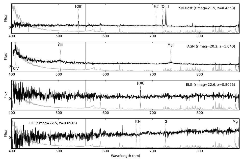
Figure 2: Sample spectra for targets of typical magnitude and redshift, with flux on a linear scale. Spectra are truncated at the blue end and smoothed by a gaussian filter of sigma 1 pixel. Key features used to measure the redshifts are marked. The spectra are not flux calibrated and the relative variance is plotted in gray. The discontinuity at 570 nm in the variance marks the dichotic split.

1. Transient: transient of any type, including supernova. Currently, an approximate $r$-band magnitude limit of 22.5, corresponding to the peak r-band magnitude of a Type Ia supernovae at $z\sim 0.5$, is imposed on the brightness of the transient. This magnitude is the limit at which we can identify a hostless Type Ia supernova with AAOmega. Because of the time-sensitive nature of transients, these objects are of the highest priority. Regardless of whether a redshift or a classification is obtained, a transient remains on the target list until it becomes fainter than the magnitude limit. There are only 5 to 10 active transients at any one time in each DES field, so all of these will be assigned a fibre unless a collision with another transient occurs.

2. AGN Reverberation: AGN candidate or previously-identified AGN that we began to monitor in Y1. The AGN candidates were selected based on photometry from DES, VHS (McMahon et al., 2013), and WISE (Wright et al., 2010) with a variety of methods (Banerji et al., 2015). The selection methods were designed to emphasize completeness over efficiency, particularly for the brightest candidates, in order to maximize the number of bright AGN. Besides brightness, we use redshift, emission-line equivalent width, and luminosity to identify targets for monitoring. For each run in Y1, approximately 150 fibers per field were devoted to AGN targets (Table 2). As Y1 progressed, a growing fraction of these fibers were devoted to the monitoring program.

3. SN Host: host galaxy of a supernova or other transient detected since the DES SV season. A host galaxy is defined as the closest galaxy in units of its effective light radius from the SN (cf. Sako et al., 2014; Sullivan et al., 2006). An allocated fibre is placed at the core of the galaxy to maximize the flux input (but see $\S$ 5.3 for a complementary strategy employed in Y2). Around 20 new hosts are identified for each DES field for each OzDES observing run. The total number of targets accumulates as fainter objects remain in the list until it becomes clear that we are unlikely to get a redshift. During the first year, no target was dropped. We are currently using these data to assess when targets should be dropped in favour of new targets.

4. White Dwarf: white dwarf candidate. The list is updated between observing runs based on analysis of the observed spectra, when successfully classified targets are dropped.

5. Strong Lens: strong lens system identified in the DES imaging. Up to five lens systems per field were targeted in Y1.

6. Cluster Galaxy: cluster galaxy selected via the redMaPPer cluster finder on the SVA1 Gold catalog (a galaxy catalog from co-added SV imaging; Rykoff et al., 2014, Rykoff et al., in prep). High probability cluster galaxies are selected to be luminous galaxies in moderately rich clusters that have a luminosity consistent with the cluster richness, as well as occupying regions with a high local density. An additional constraint of $m_{r}<22.5$ mag is put on the galaxies for AAOmega targeting. Central cluster galaxies with $0.6<z_{\mathrm{photo}}<0.9$ are given a higher priority (ClusterGalaxy I in Table 3), with the median target redshift of $0.80$. Another lower priority list of targets (ClusterGalaxy II) is made for centrals and bright satellites of clusters at $z<0.6$.

7. Radio Galaxy: galaxy selected from the ATLAS survey. Although these are labelled “Radio Galaxy” for convenience, about half the objects are star forming galaxies or radio-quiet AGN. As for cluster galaxies, we allow two priority settings, for RadioGalaxy I and RadioGalaxy II. During Y1, category II was rarely used (only two objects), so it is not listed in Table 3.

8. F star: F star candidate in Y1 (from Nov. 2013), to obtain spectroscopic classification. The goal is to have approximately 10 to 15 high signal to noise F stars per field to be used as flux calibrators. Candidates were selected in the Northern fields using photometry from SDSS that included u-band.

9. Sky: sky regions with no detectable sources in DES imaging. Approximately 25 fibres are allocated per field.

10. LRG: luminous red galaxy used to calibrate DES photometric redshifts. The high-$z$ (median$\sim$0.7) population is selected based on DES+VHS photometric data (Banerji et al., 2015).

11. ELG: emission line galaxy used to calibrate DES photometric redshifts. Color selections similar to Comparat et al. (2013) are used. For bright targets ($19<m_{i}<21.3$), $-0.2<(m_{g}-m_{r})<1.1$ and $-0.8<(m_{r}-m_{i})<1.4$; for faint targets ($21.3<m_{i}<22$), $-0.4<(m_{g}-m_{r})<0.4$, $-0.2<(m_{r}-m_{i})<1.2$ and $m_{g}-m_{r}<m_{r}-m_{i}$.

12. photo-$z$: galaxy target, selected using the DES i-band magnitude cut $17\leq m_{i}<21$, used to calibrate DES photometric redshifts.

3.4 Data Reduction

We process the data from AAOmega soon after they have been taken so that we are able to quickly determine redshifts, usually within 48 hours of them being observed and often before the next night’s observations. This gives us the chance to deselect targets if a secure redshift (see below) has been obtained and therefore free up fibres to observe other targets later in the run.

All data from AAOmega are processed with 2dfdr (Croom, Saunders & Heald, 2004). The procedure is broken into a number of steps, each of which is discussed below.

• Bias Subtraction and Bad Pixel Masking. For data taken with the blue CCD, this consists of using the overscan region to subtract the bias, subtracting a master bias to remove features that cannot be removed by using a fit to the overscan region, and subtracting a scaled version of the master dark. For the red CCD, this simply consists of using the overscan region to remove the bias. Cosmic rays are detected with an edge detection filter. The affected pixels are masked as bad throughout the subsequent analysis and are not used. Some cosmic rays sneak through this step, but are captured later when multiple exposures are combined.

• Tram line mapping and wavelength calibration. The fibre flat is used to measure the location of the fibre traces (the tram line map), while the arc is used to wavelength calibrate the path along each fibre. In future versions of 2dfdr, the fibre flat will also be used to model the fibre profile.

• Extraction. A 2d spline model of the background scattered light is then subtracted, and the flux from individual fibres is extracted. The flux perpendicular to the fibre trace is weighted with a Gaussian that has a FWHM that matches the FWHM of the fibre trace. In future versions of 2dfdr, both of these steps will be replaced with a single step that optimally extracts the flux and determines the background (Sharp & Birchall, 2010).

• Wavelength calibration. The extracted spectra are calibrated in units of constant wavelength using the arcs.

• Sky subtraction. The relative throughput of the fibres is normalised, and the sky is removed using the extracted spectrum of the sky fibres. Usually, there are residuals that remain after this step. These are removed using a principal component analysis of the residuals (Sharp & Parkinson, 2010).

• Combining and Splicing. If more than one exposure was obtained, which is usually the case, the reduced spectra are co-added. Remaining cosmic rays are found as outliers and removed at this stage. The red and blue halves of the spectra are then spliced. At this stage, we do not weight the data before we combine it. In future versions of the OzDES pipeline, we will weight the spectra and both the splicing and combining will be merged into a single step.

3.5 Redshifting

All spectra are visually inspected by OzDES team members using the interactive redshifting software runz, originally developed by Will Sutherland for the 2dFGRS. runz first attempts an automatic redshift determination by both cross-correlating to a range of galaxy and stellar templates and searching for emission line matches. It then displays the spectrum and marks the locations of the common emission and absorption features at the best redshift estimate. A redshifter visually inspects the fit and determines whether the redshift is correct. A number of interactive tools are provided, e.g. to switch to a different template, to mark a specific emission line, to add a comment, or to input the redshift directly.

Uncertainties on the redshifts are calculated by runz based on the width of the cross-correlation peak or the fit to emission lines. However, we are able to derive more representative uncertainties for various classes of objects (e.g. galaxies and AGN, see 4.2) using objects that are observed multiple times.

Each redshift is assigned a quality flag. For most objects, we use a number between 1 and 4, with a larger number meaning a more secure redshift estimate. We reserve quality flag 6 for stars.

• Quality 4 is given when there are multiple strong spectral line matches. With the exception of AGN and transients, these are removed from the target pool and are not re-observed.

• Quality 3 is given for multiple weak spectral line matches or single strong spectral line match (e.g. a bright emission line that is consistent with high-redshift [OII]). These can be used for science, but for some target types (e.g. SN hosts), may also be re-observed until the quality is deemed worthy of a 4.

• Quality 2 is given to targets where there are one or two very weak features (e.g. a single weak emission line that may be [OII]). The redshift is speculative and not reliable enough for science.

• Quality 1 is given to objects where no features can be identified.

Targets with quality 1 and quality 2 redshifts are re-observed until the deselection criteria are met.

In practice, the assignment of quality flags by a redshifter is subjective to experience and many other factors. We require independent assessments from two members of the team for each object. The results from the two redshifters are then compared by a third “expert”, who chooses the appropriate redshifts and quality flags and provides feedback to the individual redshifters. This helps to train redshifters and to homogenise the redshifting process. The number of cases where there is true disagreement is small, most disagreements arise from a difference in quality rating.

At the beginning of Y1, we set the following requirements for the reliability of the redshift:

• 6: more than 99% correct (reserved for stars)

• 4: more than 99% correct (reserved for galaxies)

• 3: more than 95% correct (for any object)

Redshifts with quality of 3 and above are considered trustworthy for science analysis, so it is important to know the actual rate of redshift blunders. By comparing objects that were observed multiple times and redshifted independently, we find that we are achieving the required level of reliability for quality flags 4 and 6, but are tracking below 95% for quality 3. These results are presented in $\S$ 4.3.

3.6 Classification of Active Transients

Timely identification is critical for transient studies. Discovery of a supernova at an early phase may trigger observations at other wavelengths or spectroscopic time series throughout its evolution. The earlier the follow-up campaign starts, the more information it will gather to understand the explosion physics. In the exciting case of an unknown type of transient, early observations may be vital for the interpretation of its true nature and the only chance to observe it if it is short-lived.

Spectral classification of a SN is usually done by comparison to templates. The best match type and age are found through either cross-correlation (e.g. the Supernova Identification, SNID, Blondin & Tonry, 2007) or chi-square minimization (e.g. Superfit, Howell et al., 2005).

During the first season of OzDES, we observed 320 transients and determined the redshifts (mostly from features of the host galaxies) of about 73% of them. Of these, 12 were positively identified as supernovae (Childress et al., 2013b; Yuan et al., 2013, 2014). This is a small fraction of all transients. There are a number or reasons for this.

First, one of the aims of OzDES is to explore the range of transient phenomena that exists in the DES deep fields, so a deliberate decision was made to target objects that were clearly not SN. This includes objects that turned out to be AGN or variable stars.

Second, the amount of host galaxy light relative to SN light that enters the $2\hbox{${}^{\prime\prime}$}$ 2dF fibre is larger than is normally the case for long slit observations, which typically use slits that are $1\hbox{${}^{\prime\prime}$}$ wide. This, coupled with the typical seeing at the AAT ($2\hbox{${}^{\prime\prime}$}$), makes the SN less clearly visible in spectra from 2dF.

Third, SN typing relies on identifying broad spectral features. At the beginning of Y1, the pipeline that was used to process the data imprinted features to the spectra (e.g. a discontinuity between the red and blue halves) that obfuscated the SN signal. Only the brightest SN in Y1 could be identified with confidence.

3.7 Ongoing improvements

While the Y1 spectra are suitable for determining redshifts, artefacts that come from the processing result in data that are less suitable for other analyses, such as the spectral typing of transients. The most common artefact is a flux discontinuity in the overlap region between the red and blue halves of the spectra.

Since the first year of the OzDES campaign, considerable work has gone into mitigating these artefacts by improving the algorithms in 2dfdr. These improvements include better tramline tracking, implementation of optimal extraction (which leads to more accurate treatment of the background scattered light), better flat fielding, more effective cosmic ray removal and improved flux calibration. During Y1, we have used the sensitivity functions provided with 2dfdr to do the flux calibration. In future versions of the OzDES pipeline, we will use the F stars that are observed contemporaneously with the other targets to do the flux calibration. Absolute calibration will be done using the broad band DES photometry.

Not all of the above algorithms are implemented at once, but better data reduction has already helped us to classify 50% more SNe in Y2 than in Y1. Reprocessing of the entire OzDES data set from Y1 and Y2 is planed, after which redshifts and spectra will be publicly released (Childress et al. in prep).

4 Results

During Y1 and SV, 10482 unique targets were observed and 6727 redshifts (with quality flag 3 and above) were obtained. Figure 3 shows the redshift distributions for selected targets. The fraction of objects with measured redshifts and their number are listed in Table 3 for each type of target. For selected groups of extragalactic objects, we also show the completeness of redshifts as a function of integrated magnitude within the fibre diameter (Figure 4). For non-transient objects, photometry measurements are taken from the DES SV Gold catalog (Rykoff et al., in prep). For transients, the magnitude does not include the flux of the underlying host and represents luminosity measured in the last epoch when the target was selected.

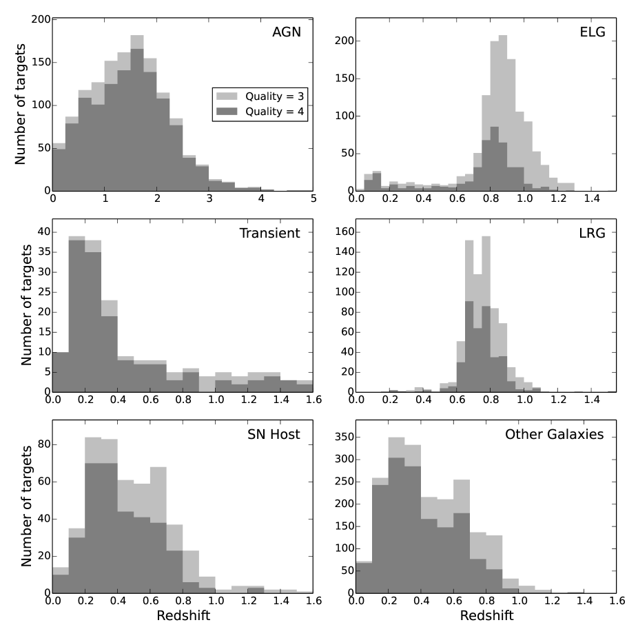
Figure 3: Redshift distributions for selected target types. Objects that have redshifts consistent with Galactic origins are excluded. Dark shaded histograms represent objects with redshift quality flag of 4 (most reliable; see $\S$ 3.5) and the light shaded histograms represent objects with redshift quality flag of 3 (reliable). Other galaxies include radio galaxies, cluster galaxies and galaxies that are specifically chosen to calibrate photometric redshifts. Redshift bins are set to be smaller for ELGs and LRGs to provide higher resolutions around the peak.

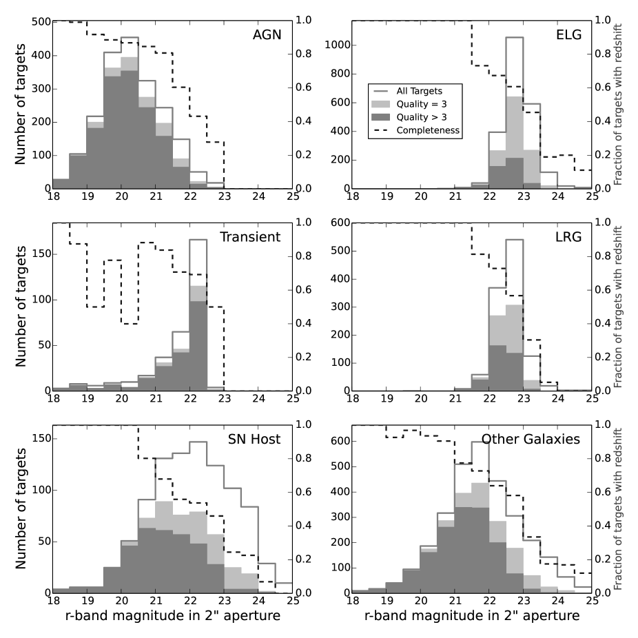
Figure 4: Redshift completeness as functions of r-band magnitude measured in a $2\hbox{${}^{\prime\prime}$}$ diameter aperture, for selected groups of extragalactic objects. Unfilled histograms are for all targets. Dark shaded histograms represent objects with redshift quality of 4 and above (most reliable; see $\S$ 3.5). Light shaded histograms represent objects with redshift quality of 3 (reliable). Completeness (as dashed curves) is defined as the fraction of objects for which redshifts are measured with quality flag 3 and above. The magnitude range is fixed for all panels for easy comparison. A few galaxies in the bottom two panels have measured magnitudes fainter than 25. These bins have low completeness and are excluded to emphasize the more typical magnitude range.

4.1 Efficiency and Completeness

As expected, the probability of a successful redshift measurement drops for fainter targets. This trend is weak for the transients because the redshifts of most transients are inferred from spectral features of their hosts. Strength of such features depends on the host luminosity, redshift and location of the transient relative to its host.

The redshift efficiency is the likelihood of measuring a redshift above a certain quality level in a given observation time. Difference in completeness during comparable integration times reflects difference in efficiency for different types of targets. In general, emission lines allow measurements of redshift for sources with faint continuum, while cross-correlation for a galaxy without identifiable emission features relies on well measured spectral shape, combined with absorption features that are usually relatively weak, and therefore needs brighter continuum. Hence, for ELGs, the efficiency is less sensitive to the integrated broad-band magnitude than for the LRGs.

In practice, the ELGs are selected to be at $z\sim 1$, so only the [OII] $\lambda\lambda$ 3726,3728 doublet is within our wavelength range. This double line appears blended at the resolution of our spectra, and although it can often be recognized as a wide or flat-topped line, it is a single feature that is prone to misidentification. It is hard for redshifters to say conclusively that it is [OII] and not another line or an artefact. A high fraction of the ELGs are therefore rated at a redshift quality of 3.

The nominal target type is known to the redshifter. For ELGs, LRGs and AGN, this may cause the redshifter to assign a higher redshift quality flag than would be the case if the target type was not available to the redshifter.

SN hosts show lower completeness across a wide magnitude range than either ELGs or LRGs (see Figure 4). This sample is selected based on criteria independent of whether the galaxy is of early or late type. The redshift range may be constrained by the selection criteria, but knowing the target type does not directly help in determining a redshift.

At a given magnitude, the redshift completeness grows with integration time. Many of the faint targets are expected to be observed in multiple seasons and accumulate significantly more signal than obtained so far. The data from Y1 do not have sufficient range of exposure time to determine this trend with much certainty. In O’Neill et al. (in prep), we use data gathered by the end of Y2 to model how the number of redshifts acquired increase as a function of number of visits to the field, for various types of targets with different magnitude and redshift distributions. We then estimate the redshift completeness of the survey and the number of objects we are likely to observe by extrapolating to a total of 25 visits. We are on track to obtain redshifts for 80% of all SN host galaxies that are targeted.

4.2 Redshift Precision

Estimates of the redshift precision based on emission line fitting or template cross-correlation may suffer different biases. For almost all of our target groups, a combination of techniques has been used. It is recognized that for most of our science cases, we exceed the minimum requirement of precision. Therefore, we do not attempt to assign accurate uncertainties for individual redshift measurements, but instead provide an overall statistical error estimate for classes of targets, based on the dispersion in measured redshifts for individual objects with multiple independent measurements, either from different observing runs or from appearing in the overlap regions of the DES fields. Objects with inconsistent redshift measurements are excluded (see next section). For each object, we calculate the pair-wise differences of these redshifts, divided by $1+z_{\rm median}$. The distributions are examined for several populations of extra-galactic objects. We quote the 68 percent ($\sigma_{68}$) and 95 percent ($\sigma_{95}$) inclusion regions in Table 4, since the distributions have extended tails. Typical uncertainties ($\sigma_{68}$) for AGN and galaxies are 0.0015 and 0.0004 respectively.

We also compare our results against the redshifts from other surveys covering our targeted sky area. Only redshifts with the most confident quality flag defined by the corresponding survey are considered. The results are listed in Table 4 as “external”. No significant systematic offset is found between OzDES and surveys such as GAMA (Driver et al., 2011) or SDSS (Ahn et al., 2014). Distributions of the differences between our redshifts and those from other surveys are consistent with the internal comparisons.

A large number of AGN were targeted repeatedly from run to run by design. This allows us to split the sample and quote the uncertainties in two redshift bins. The redshifts of AGN are often measured by cross-correlating with template spectra. Due to intrinsic variation of the emission profiles from AGN to AGN, the precision of a measurement depends on the quality of the template, the wavelength region included in the cross-correlation and/or the line chosen by the redshifter to centre on. At redshift one and above, high ionization emission lines with large profile variation, such as CIII] or CIV are often used, resulting in larger uncertainties in the redshifts.

The number of repeated observations is small for all other galaxy targets as they are usually removed when secure redshifts are obtained. To investigate possible type dependence, we examine separately the dispersions for ELG, LRG and SN host targets. The smaller dispersion for the ELGs is consistent with the expectation that better constraints can be obtained from narrow emission lines.

4.3 Redshift Reliability

For a quantitative evaluation of the reliability of our redshifts, we compare multiple redshifts obtained for the same objects from independent observations, either from different observing runs or from appearing in the overlap regions of the DES fields. For each redshift, we calculate its offset from a redshift that is deemed to be correct. For simplicity, we call this value the base redshift. We elaborate on how the base value is determined below. A redshift is considered wrong if it differs from the base redshift by more than $0.02(1+z)$ for a AGN or $0.005(1+z)$ for a galaxy, which are roughly ten times the standard deviations measured from the previous section.

The base redshift can be obtained from either internal or external sources. Internally, if a redshift with a higher quality flag exists, we consider that redshift as the base redshift. Otherwise, the median value is used if more than two redshifts are available or a random selection is made assuming at least one measurement is correct. The external redshifts are chosen from other surveys to have the highest quality flag defined. When a conflict between an OzDES redshift and an external redshift is found, the OzDES spectra are re-examined. In three cases (for quality 3 AGN), the data quality is not good enough to confirm either redshift. These are excluded in the calculations.

As shown in Table 4, overall close to 100% of redshifts are correct with quality flag 4 but only about 90% of redshifts are correct with quality flag 3. To better understand the sources of error, we examine different galaxy types separately. The relatively high error rate for SN hosts (more than 15% for quality 3) possibly arises because of the diversity of objects that host supernovae. The ELG sample appears more homogeneous.

As noted earlier, the error rate for quality 3 objects is higher than our goal of 5%. After Y1, we implemented a number of changes (better training of the human redshifters and more scrutiny of quality 3 objects by the third person) that have resulted in fewer errors.

With increasing experience and better data processing, further improvements on the reliability and the quality of the redshifts are expected in the coming seasons and will be closely monitored.

Table 4: Redshift uncertainties and error rates. Uncertainties are calculated using weighted pair-wise redshift differences, $\Delta z/(1+z)$, for objects observed in multiple overlapping fields or multiple observing runs ($\S$ 4.2). A redshift is considered wrong if it differs from a chosen base redshift ($\S$ 4.3) by more than $0.02(1+z)$ for a AGN or $0.005(1+z)$ for a galaxy.

Type	Number of redshift pairs	$\sigma_{68}$*	$\sigma_{95}$*	Error rate (Q = 4)	Error rate (Q = 3)
AGN	-	-	-	1/1647 (0.1%)	22/388 (5.7%)
AGN ($z\leq 1$)	521	0.0004	0.0011	-	-
AGN ($z>1$)	1568	0.0015	0.0038	-	-
AGN (external)	424	0.0016	0.0048	0/387 (0.0%) $\ddagger$	6/46(13.0%)$\S$
Galaxy$\dagger$	99	0.0004	0.0013	0/74 (0.0%)	10/95 (10.5%)
ELG	25	0.0002	0.0006	0/8 (0.0%)	2/32 (6.3%)
LRG	21	0.0005	0.0013	0/16 (0.0 %)	3/20 (15.0%)
SN host	36	0.0003	0.0013	0/38 (0.0%)	4/25 (16.0%)
Galaxy (external)	182	0.0004	0.0010	0/159 (0.0%)$\parallel$	0/24 (0.0%)
*68 percent ($\sigma_{68}$) and 95 percent ($\sigma_{95}$) inclusion regions.
$\dagger$All types of galaxy targets that are not AGN.
$\ddagger$In three cases of discrepancy, spectra are inspected and the OzDES measurements are confirmed to be correct.
$\S$All discrepant redshifts are checked by hand. Objects are excluded if the available data is not good enough to confirm either
redshift measurement.
$\parallel$In one case of discrepancy, spectra are inspected and the OzDES measurement is confirmed to be correct.

5 Discussion and highlights

In this section, we present updates on some of our key science goals in light of the results from Y1. When necessary, complementary data taken in Y2 are included to demonstrate the potential of our observing strategy. Some of the discussions involve changes in Y2 that are inspired by analysis of the Y1 data.

5.1 SN Ia Cosmology

The DES SN survey strategy is optimized to detect a large number of SNe Ia with a redshift distribution that extends to redshift 1.2 and peaks around redshift 0.6 (cf. Figure 10 of Bernstein et al., 2012). Since host galaxy redshifts from OzDES will be the main source of redshifts for Hubble Diagram analyses, the efficiency of obtaining redshifts by OzDES will affect the actual redshift distribution in addition to the discovery efficiency of DES.

In practice, SNe Ia candidates are first selected based on DES light-curves and photo-$z$ of putative host galaxies. The host galaxies of these candidates are then targeted by OzDES. Any redshifts obtained are subsequently used to refine the selection. Only those SNe Ia with a secure host spectroscopic redshift are considered further for cosmology studies. The combined efficiency of this process can be evaluated by comparing the selected SNe Ia sample to a simulated population. From the DES Y1 data, we select SNe that satisfy light curve quality cuts defined in Table 6 of Bernstein et al. (2012), with the exception that only two filters are required to have maximum signal-to-noise above 5 (i.e. 2 filters with SNRMAX $>$ 5). The looser cuts are compensated for by additional selection criteria on peak color and SALT2 (Guy et al., 2007) model fit parameters ($x1$ and color) to achieve $>$ 96% purity (tuned for simulation, cf. Gjergo et al., 2013). We show in Figure 5 the redshift distribution of the selected SNe Ia for which host spectroscopic redshifts are available by end of Y2. The median redshift of this observed sample is 0.52, compared to a median redshift of 0.63 for SNe Ia selected with the same photometric criteria from a SNANA (Kessler et al., 2009) simulation with realistic survey characteristics (e.g. observing cadence, seeing conditions and photometry zero points) from Y1 as input. The lower median redshift for the observed sample is mainly due to the difficulty of measuring redshifts in more distant and fainter galaxies. In the two deep fields (C3 and X3), half of the SNe Ia host galaxies are fainter than 24th magnitude in r-band and the overall redshift completeness is only about half of that for the shallow fields.

With longer exposure times, the redshift completeness will improve at all redshifts. Only for the most distant SNe, spectroscopic redshifts may remain scarce for host galaxies at typical brightness. This bias against faint host galaxies needs to be considered as it has been shown that stretch and color-corrected SN Ia peak magnitude depend on the host galaxy stellar mass (e.g. Kelly et al., 2010; Sullivan et al., 2010; Lampeitl et al., 2010; Childress et al., 2013a).

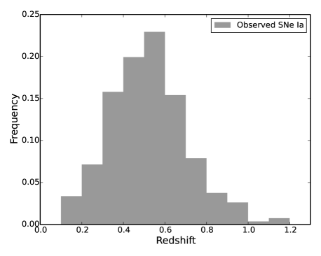
Figure 5: Normalized redshift distribution of selected SNe Ia candidates from Y1 that have host spectroscopic redshifts. The selection criteria are tuned to achieve $>$ 96% purity (see text in $\S$ 5.1). The median redshift of this sample is 0.52.

5.2 Faint SN hosts and Spectra Stacking

As discussed above, high redshift efficiency across a wide brightness range is critical to maximize the statistics and minimize the bias of a sample of SNe with host galaxy spectroscopic redshifts. Such a goal is achieved by OzDES’s unique strategy of repeat targeting, dynamic fibre allocation, and stacking. Multiple observations of the same DES field allows dynamic control of effective exposure times for targets of different brightness. The brighter galaxies are deselected between the observing runs when redshifts are measured; while fainter galaxies remain in the queue. Stacking across many observing runs allows OzDES to go deeper than otherwise possible with the 3.9m AAT. Figure 6 shows an example of stacked spectra, for a SN host target of r-band magnitude 23.7 and redshift 0.732. The growing significance of the emission line, roughly consistent with square root of exposure time, supports the credibility of the feature.

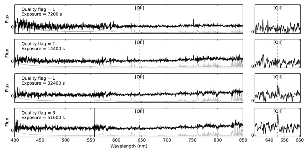
Figure 6: Selected co-added spectra of a SN host target of r-band magnitude 23.7 and redshift 0.732. The significance of the candidate [OII] feature appears to have increased with exposure time. A quality flag of 3 is assigned so the target will remain in the queue until more data confirms the redshift.

5.3 Hostless SNe and Super-Luminous SNe

We showed in $\S$ 4.1 that redshift efficiency has a different dependence on target brightness for different types of galaxies. The likelihood of measuring an emission line redshift is less sensitive to apparent broad-band luminosity. A significant fraction of SNe (including most SNe Ia and most core-collapse SNe) are expected to occur in star-forming regions. For some, strong emission lines may show up in dispersed AAT spectra even though the continuum is too faint to be detected by DECam imaging in the first few seasons. A new strategy of targeting hostless SN, by placing a fibre at the position of a SN after the transient has faded, is implemented after Y1 and has already yielded redshifts that would otherwise be elusive.

This strategy is particularly interesting for validating Super-Luminous SN (SLSN) candidates. SLSNe are a rare and extreme class of SN discovered in recent years (Gal-Yam, 2012). The origin of SLSNe are unclear, but they play a key role in understanding the evolution of massive stars, chemical enrichment and possibly cosmic re-ionization via their bright UV luminosity. DES will discover many of these intrinsically bright objects out to redshift about 2.5 (Papadopoulos et al., 2015). At high redshifts, the optical (rest-frame UV) spectra of the SLSNe are poorly understood. Redshifts from host galaxies are thus crucial to constrain their distances and intrinsic luminosities. However, SLSNe preferentially occur in dwarf star-forming galaxies (Lunnan et al., 2014), many of which are too faint to be detected or to have reliable photo-$z$ estimates from DES multi-band imaging. OzDES provides a cost-effective inspection as the number of SLSN candidates is large with respect to the time available on 8 to 10m class telescope but is small compared to the number of AAT fibres. These SLSNe targets will gain high priority in future AAT observing seasons.

5.4 AGN

We obtained almost 6000 spectra of AGN and AGN candidates in Y1 (see $\S$ 3.3 for details on the target selection strategy and Figure 2 for an example spectrum). After the completion of Y1, we identified 989 AGN to monitor. The number of AGN targets decreases from 150 per field to 100 per field, but the priority is maintained at 7 to ensure that the object is observed as frequently as possible.

The median redshift of these AGN is 1.63 and the distribution extends to z$\sim$4.5 (see Figure 7). The sample will primarily be analyzed using either the Mg ii@ or Civ@ emission line, and in some cases both lines. We will also monitor a substantial number of targets using the $H\beta$ emission line, which is the most commonly used line in previous reverberation mapping campaigns (e.g. Peterson et al., 2004). We expect to accurately recover the radius-luminosity relationship for all three lines (King et al., in prep).

Based on data obtained from Sept. 2013 through the end of 2014, we presently have 5 (6) or more spectroscopic epochs for 693 (455) AGN (70% and 46% of the sample). These numbers are close to the expected 7 epochs (in the first two seasons) for 500 AGN in our survey simulation (King et al., in prep). For more than 10% of the sample, we have acquired spectra in 8 epochs.

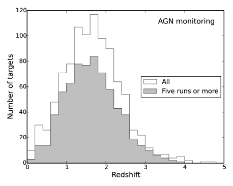
Figure 7: Redshift distribution of the AGN being monitored after the first year. Shaded area represents objects that have been observed in 5 runs or more by the end of 2014.

5.5 Radio Galaxies

By the end of Y1, we had observed 350 targets from the first data release of the ATLAS survey (Norris et al., 2006; Middelberg et al., 2008), augmenting the earlier work of Mao et al. (2012). Secure redshifts were obtained for 40% of the targeted sources and the majority currently without redshifts are fainter than $m_{r}=22.5$ mag. Sources without a redshift will be re-observed in coming campaign seasons to build up the necessary integration time to determine their redshifts and classifications. As we continue to observe these targets, we expect to increase our completeness.

With the availability of the ATLAS data release 3 (Franzen et al. in prep, Banfield et al. in prep), target selection has been modified slightly after Y1. The additional post-processing provides higher detection reliability at low radio flux levels leading to increased sensitivity to low-level star formation.

The redshifts obtained will be used to further the science goals for ATLAS including:

• to determine the cosmic evolution of both star forming galaxies and radio AGN, through the measurement of their redshift-dependent radio luminosity functions. For example, we will be able to measure luminosity functions for star-forming galaxies to $\sim L$* (the expected knee of the luminosity function at $z$=1).

• to calibrate and develop photometric and statistical redshift algorithms for use with the 70 million EMU (Norris et al., 2011) sources (for which spectroscopy is impractical).

• to measure line widths and ratios of emission lines to distinguish star forming galaxies from AGN, low-ionization nuclear emission-line regions (LINERs), etc, and identify quasars and broad-line radio galaxies.

• to measure how radio polarisation evolves with redshift, as a potential measure of cosmic magnetism.

• to explore how morphology and luminosity of radio-loud AGN evolve with redshift, to understand the evolution of the jets and feedback mechanisms.

5.6 Unusual Objects

The large number of spectra taken by OzDES almost guarantees discoveries of rare events or objects. Even in the photometrically selected samples, outliers are expected to exist. Although an exhaustive search for unusual objects is beyond the scope of this work, we highlight this potential by noting some objects that clearly stand out when the spectra were visually inspected in runz. These objects fall in the following broad categories:

1. Unusual transients: Time sensitive observations of live transients are of high priority. To maximize the discovery space, we target all transients that satisfy a straightforward magnitude cut. As discussed in $\S$ 3.6, studies of transient spectra have been complicated by host galaxy light contamination and data reduction issues. A more systematic investigation will be carried out when data reduction is refined.

2. Rare stars: At least four WD and M-dwarf binaries are recognized as Galactic objects with both a hot and a cool spectral components. We have also found a WD candidate that is likely a rare DQ WD (with carbon bands).

3. Serendipitous spectroscopic SN: A SN may be observed unintentionally for two reasons. It happens to occur in a galaxy where a redshift is desired or it is mis-classified into a different target type. During the SV season, one of the photo-$z$ targets turned out to be a Type II SN. The chance for this to happen drops significantly in subsequent seasons as long-term photometry becomes available. However, the first possibility becomes more likely as more galaxies are targeted. Approximately one SN occurs every century in a Milky Way-like galaxy and a SN remains bright for a few weeks to a few months. It is thus expected that every few thousand galaxy spectra at relatively low redshift may contain a visible SN. The concept of spectroscopic SN search has been successfully tested (Madgwick et al., 2003; Graur & Maoz, 2013). However, such a survey method requires more than human eyes because the host galaxy light often dominates and has to be carefully modeled.

4. Broad Absorption Line (BAL) AGN: A large number of AGN are observed as reverberation mapping targets, radio sources, galaxies or transients. More than a dozen of these exhibit extraordinary absorption line systems. Selected objects will be monitored throughout our survey.

5. Multiple redshifts: If two objects fall in the same fibre, two distinct sets of spectral features may be observed. Searching for double redshifts in galaxy spectra provides a way of finding strong gravitational lens candidates (e.g. Bolton et al., 2004), particularly for small Einstein radii and faint background sources that are hard to detect by imaging. Four OzDES targets were noticed to show convincing features at two different extra-galactic redshifts. Inspection of the images reveal that two of these are merely chance alignment between background sources and foreground galaxies. The remaining two systems are lens candidates, both consisting of a foreground early type galaxy and a background emission line galaxy.

6 Conclusions

OzDES is an innovative spectroscopic program that brings together the power of multi-fibre spectrograph and time-series observations. In five years, each DES SN survey field will be targeted in about 25 epochs during the DES observing seasons by the 2dF/AAOmega spectrograph on the AAT. The 400 fibres are configured nightly to target a range of objects with the goal of measuring spectroscopic redshifts of galaxies, monitoring spectral evolution of AGN or classifying transients. Stacking of multi-epoch spectra allows OzDES to measure redshifts for galaxies that are as faint as $m_{r}=25$ mag. Along with efficient redshifting and recycling of fibres, we expect to obtain about 2,500 host galaxy redshifts for the DES SN cosmology study. The long term time series, contemporaneous with DECam imaging, will enable reverberation mapping of the largest AGN sample to date. In addition, OzDES is an important source of redshifts for various DES photo-$z$ programs.

In the above sections, we have summarized the OzDES observing strategy, reported results from the first year of operation and evaluated the outcome in light of various science goals. Overall, our strategy has worked well in the first year and produced a large number of redshifts with good quality. We are on track to achieve our main science goals. Meanwhile, we have identified a number of areas for improvements, including better data reduction procedures to reduce artefacts and more rigorous cross-check to raise redshift reliability.

By the time of writing, the second observing season (Y2) has completed and already a number of updates have been implemented. Additional data and better understanding of the survey yield has allowed us to reassess target selection and de-selection criteria for different target types and science goals. For example, targeting the brightest objects first maximizes the number of measured redshifts for radio galaxies, but such tactics only work when selection bias is not a major consideration. It is also desirable to abandon an unsuccessful target after certain number of exposures while the maximum integration time allowed depends on the total number of redshifts anticipated for this particular target type. Short integration times allow faster recycling of fibres and more redshifts to be measured. During poor observing conditions, a backup program is in place to measure redshifts for bright galaxies, along with high priority targets such as AGN and active transients.

As for all long-term projects, we expect to continue to refine our data quality, actively analyze new data and adapt the observing strategy in the coming years.

Affiliations

¹Research School of Astronomy and Astrophysics, The Australian National University, Canberra, ACT 2611, Australia
²ARC Centre of Excellence for All-sky Astrophysics (CAASTRO)
³Australian Astronomical Observatory, North Ryde, NSW 2113, Australia
⁴School of Mathematics and Physics, University of Queensland, QLD 4072, Australia
⁵Department of Physics & Astronomy, University College London, Gower Street, London WC1E 6BT, UK
⁶Kavli Institute for Cosmology, University of Cambridge, Madingley Road, Cambridge CB3 0HA, UK
⁷Institute of Astronomy, University of Cambridge, Madingley Road, Cambridge CB3 0HA, UK
⁸Fermi National Accelerator Laboratory, P.O. Box 500, Batavia, IL 60510 USA
⁹Observatório Nacional, Rua Gal. José Cristino 77, Rio de Janeiro, RJ - 20921-400, Brazil
¹⁰Laboratório Interinstitucional de e-Astronomia - LIneA, Rua Gal. José Cristino 77, Rio de Janeiro, RJ - 20921-400, Brazil
¹¹Department of Physics and JINA Center for the Evolution of the Elements, University of Notre Dame, 225 Nieuwland Science Hall, Notre Dame, IN 46556, USA
¹²INAF- Astrophysics Observatory of Turin , Strada Osservatorio 20, Pino Torinese, Torino, 10025, Italy
¹³Institut de Ciències de l’Espai, IEEC-CSIC, Campus UAB, Facultat de Ciències, Torre C5 par-2, 08193 Bellaterra, Barcelona, Spain
¹⁴Institute of Cosmology and Gravitation, University of Portsmouth, Dennis Sciama Building, Burnaby Road, Portsmouth, PO1 3FX, UK
¹⁵Kavli Institute for Particle Astrophysics & Cosmology, P. O. Box 2450, Stanford University, Stanford, CA 94305, USA
¹⁶Department of Astronomy, University of Illinois at Urbana-Champaign, 1002 W. Green St., Urbana, IL 61801, USA
¹⁷Department of Physics, University of Illinois at Urbana-Champaign, 1110 W. Green St., Urbana, IL 61801, USA
¹⁸Kavli Institute for Cosmological Physics, University of Chicago, Chicago, IL 60637, USA
¹⁹Centre for Astrophysics and Supercomputing, Swinburne University of Technology, Hawthorn, VIC 3122, Australia
²⁰Lawrence Berkeley National Laboratory, 1 Cyclotron Road, Berkeley, CA 94720, USA
²¹Dark Cosmology Centre, Niels Bohr Institute, University of Copenhagen, Juliane Maries Vej 30, DK-2100 Copenhagen, Denmark
²²Argonne National Laboratory, 9700 South Cass Avenue, Lemont, IL 60439, USA
²³Sydney Institute for Astronomy, School of Physics, A28, The University of Sydney, NSW, 2006, Australia
²⁴Center for Cosmology and Astro-Particle Physics, The Ohio State University, Columbus, OH 43210, USA
²⁵Department of Astronomy, The Ohio State University, Columbus, OH 43210, USA
²⁶CSIRO Astronomy & Space Science, Epping, NSW 1710, Australia
²⁷CAPES Foundation, Ministry of Education of Brazil, Brasília - DF 70040-020, Brazil
²⁸Astronomy Centre, University of Sussex, Falmer, Brighton, BN1 9QH, UK
²⁹SLAC National Accelerator Laboratory, Menlo Park, CA 94025, USA
³⁰Department of Physics, University of Arizona, 1118 E 4th St, Tucson, AZ 85721, USA
³¹Department of Physics and Astronomy, University of Pennsylvania, Philadelphia, PA 19104, USA
³²School of Physics and Astronomy, University of Southampton, Southampton, SO17 1BJ, UK
³³Department of Physics, Stanford University, 382 Via Pueblo Mall, Stanford, CA 94305, USA
³⁴Cerro Tololo Inter-American Observatory, National Optical Astronomy Observatory, Casilla 603, La Serena, Chile
³⁵Institut d’Astrophysique de Paris, Univ. Pierre et Marie Curie & CNRS UMR7095, F-75014 Paris, France
³⁶National Center for Supercomputing Applications, 1205 West Clark St., Urbana, IL 61801, USA
³⁷George P. and Cynthia Woods Mitchell Institute for Fundamental Physics and Astronomy, and Department of Physics and Astronomy, Texas A & M University, College Station, TX 77843-4242, USA
³⁸Department of Physics, Ludwig-Maximilians-Universität, Scheinerstr. 1, 81679, München, Germany
³⁹Jet Propulsion Laboratory, California Institute of Technology, 4800 Oak Grove Dr., Pasadena, CA 91109, USA
⁴⁰Department of Physics, University of Michigan, Ann Arbor, Michigan 48109, USA
⁴¹Max-Planck-Institut für extraterrestrische Physik, Giessenbachstr. 85748 Garching, Germany
⁴²University Observatory Munich, Scheinerstrasse 1, 81679 Munich, Germany
⁴³Department of Physics, The Ohio State University, Columbus, OH 43210, USA
⁴⁴ICRA, Centro Brasileiro de Pesquisas Físicas, Rua Dr. Xavier Sigaud 150, CEP 22290-180, Rio de Janeiro, RJ, Brazil
⁴⁵Department of Astronomy, University of Michigan, Ann Arbor, MI 48109, USA
⁴⁶Institut de Física d’Altes Energies, Universitat Autònoma de Barcelona, E-08193 Bellaterra, Barcelona, Spain
⁴⁷Institució Catalana de Recerca i Estudis Avançats, E-08010 Barcelona, Spain
⁴⁸Brookhaven National Laboratory, Bldg 510, Upton, NY 11973, USA
⁴⁹Centro de Investigaciones Energéticas, Medioambientales y Tecnológicas (CIEMAT), Avda. Complutense 40, Madrid, Spain

References

- Ahn et al. (2014) Ahn C. P. et al., 2014, ApJS, 211, 17
- Banerji et al. (2015) Banerji M. et al., 2015, MNRAS, 446, 2523
- Bentz et al. (2013) Bentz M. C. et al., 2013, ApJ, 767, 149
- Bernstein et al. (2012) Bernstein J. P. et al., 2012, ApJ, 753, 152
- Blandford & McKee (1982) Blandford R. D., McKee C. F., 1982, ApJ, 255, 419
- Blondin & Tonry (2007) Blondin S., Tonry J. L., 2007, ApJ, 666, 1024
- Bolton et al. (2004) Bolton A. S., Burles S., Schlegel D. J., Eisenstein D. J., Brinkmann J., 2004, AJ, 127, 1860
- Brough, Green & Bryant (2014) Brough S., Green A., Bryant J., 2014, AAObserver, 126, 15
- Childress et al. (2013a) Childress M. et al., 2013a, ApJ, 770, 108
- Childress et al. (2013b) Childress M. et al., 2013b, The Astronomer’s Telegram, 5568, 1
- Comparat et al. (2013) Comparat J. et al., 2013, MNRAS, 428, 1498
- Croom, Saunders & Heald (2004) Croom S., Saunders W., Heald R., 2004, AAO Newsletter, 106, 12
- Davies et al. (2006) Davies R. I. et al., 2006, ApJ, 646, 754
- Diehl et al. (2014) Diehl H. T. et al., 2014, in Society of Photo-Optical Instrumentation Engineers (SPIE) Conference Series, Vol. 9149, Society of Photo-Optical Instrumentation Engineers (SPIE) Conference Series, p. 0
- Diehl et al. (2012) Diehl H. T. et al., 2012, Physics Procedia, 37, 1332
- Driver et al. (2011) Driver S. P. et al., 2011, MNRAS, 413, 971
- Flaugher (2005) Flaugher B., 2005, International Journal of Modern Physics A, 20, 3121
- Flaugher et al. (2012) Flaugher B. L. et al., 2012, in Society of Photo-Optical Instrumentation Engineers (SPIE) Conference Series, Vol. 8446, Society of Photo-Optical Instrumentation Engineers (SPIE) Conference Series, p. 11
- Gal-Yam (2012) Gal-Yam A., 2012, Science, 337, 927
- Gjergo et al. (2013) Gjergo E., Duggan J., Cunningham J. D., Kuhlmann S., Biswas R., Kovacs E., Bernstein J. P., Spinka H., 2013, Astroparticle Physics, 42, 52
- Graur & Maoz (2013) Graur O., Maoz D., 2013, MNRAS, 430, 1746
- Grier et al. (2013) Grier C. J. et al., 2013, ApJ, 773, 90
- Guy et al. (2007) Guy J. et al., 2007, A&A, 466, 11
- Howell et al. (2005) Howell D. A. et al., 2005, ApJ, 634, 1190
- Kaspi et al. (2007) Kaspi S., Brandt W. N., Maoz D., Netzer H., Schneider D. P., Shemmer O., 2007, ApJ, 659, 997
- Kelly et al. (2010) Kelly P. L., Hicken M., Burke D. L., Mandel K. S., Kirshner R. P., 2010, ApJ, 715, 743
- Kessler et al. (2009) Kessler R. et al., 2009, PASP, 121, 1028
- King et al. (2014) King A. L., Davis T. M., Denney K. D., Vestergaard M., Watson D., 2014, MNRAS, 441, 3454
- Lampeitl et al. (2010) Lampeitl H. et al., 2010, ApJ, 722, 566
- Lewis et al. (2002) Lewis I. J. et al., 2002, MNRAS, 333, 279
- Lidman et al. (2013) Lidman C. et al., 2013, PASA, 30, 1
- Lunnan et al. (2014) Lunnan R. et al., 2014, ApJ, 787, 138
- Madgwick et al. (2003) Madgwick D. S., Hewett P. C., Mortlock D. J., Wang L., 2003, ApJ, 599, L33
- Mao et al. (2012) Mao M. Y. et al., 2012, MNRAS, 426, 3334
- McMahon et al. (2013) McMahon R. G., Banerji M., Gonzalez E., Koposov S. E., Bejar V. J., Lodieu N., Rebolo R., VHS Collaboration, 2013, The Messenger, 154, 35
- Middelberg et al. (2008) Middelberg E. et al., 2008, AJ, 135, 1276
- Norris et al. (2006) Norris R. P. et al., 2006, AJ, 132, 2409
- Norris et al. (2011) Norris R. P. et al., 2011, PASA, 28, 215
- Olmstead et al. (2014) Olmstead M. D. et al., 2014, AJ, 147, 75
- Onken et al. (2014) Onken C. A. et al., 2014, ApJ, 791, 37
- Papadopoulos et al. (2015) Papadopoulos A. et al., 2015, MNRAS, 449, 1215
- Peterson (1993) Peterson B. M., 1993, PASP, 105, 247
- Peterson et al. (2004) Peterson B. M. et al., 2004, ApJ, 613, 682
- Rykoff et al. (2014) Rykoff E. S. et al., 2014, ApJ, 785, 104
- Sako et al. (2014) Sako M. et al., 2014, ArXiv e-prints
- Sako et al. (2011) Sako M. et al., 2011, ApJ, 738, 162
- Sánchez et al. (2014) Sánchez C. et al., 2014, MNRAS, 445, 1482
- Sharp & Birchall (2010) Sharp R., Birchall M. N., 2010, PASA, 27, 91
- Sharp & Parkinson (2010) Sharp R., Parkinson H., 2010, MNRAS, 408, 2495
- Shen et al. (2015) Shen Y. et al., 2015, ApJS, 216, 4
- Smith et al. (2004) Smith G. A. et al., 2004, in Society of Photo-Optical Instrumentation Engineers (SPIE) Conference Series, Vol. 5492, Ground-based Instrumentation for Astronomy, Moorwood A. F. M., Iye M., eds., pp. 410–420
- Sullivan et al. (2010) Sullivan M. et al., 2010, MNRAS, 406, 782
- Sullivan et al. (2006) Sullivan M. et al., 2006, ApJ, 648, 868
- Watson et al. (2011) Watson D., Denney K. D., Vestergaard M., Davis T. M., 2011, ApJ, 740, L49
- Woo et al. (2010) Woo J.-H. et al., 2010, ApJ, 716, 269
- Wright et al. (2010) Wright E. L. et al., 2010, AJ, 140, 1868
- Yuan et al. (2013) Yuan F. et al., 2013, The Astronomer’s Telegram, 5642, 1
- Yuan et al. (2014) Yuan F. et al., 2014, The Astronomer’s Telegram, 5757, 1