Analysis of a Classical Matrix Preconditioning Algorithm

Abstract.

We study a classical iterative algorithm for balancing matrices in the $L_{\infty}$ norm via a scaling transformation. This algorithm, which goes back to Osborne and Parlett & Reinsch in the 1960s, is implemented as a standard preconditioner in many numerical linear algebra packages. Surprisingly, despite its widespread use over several decades, no bounds were known on its rate of convergence. In this paper we prove that, for any irreducible $n\times n$ (real or complex) input matrix $A$, a natural variant of the algorithm converges in $O(n^{3}\log(n\rho/\varepsilon))$ elementary balancing operations, where $\rho$ measures the initial imbalance of $A$ and $\varepsilon$ is the target imbalance of the output matrix. (The imbalance of $A$ is $\max_{i}|\log(a_{i}^{\text{out}}/a_{i}^{\text{in}})|$, where $a_{i}^{\text{out}},a_{i}^{\text{in}}$ are the maximum entries in magnitude in the $i$th row and column respectively.) This bound is tight up to the $\log n$ factor. A balancing operation scales the $i$th row and column so that their maximum entries are equal, and requires $O(m/n)$ arithmetic operations on average, where $m$ is the number of non-zero elements in $A$. Thus the running time of the iterative algorithm is $\widetilde{O}(n^{2}m)$. This is the first time bound of any kind on any variant of the Osborne-Parlett-Reinsch algorithm. We also prove a conjecture of Chen that characterizes those matrices for which the limit of the balancing process is independent of the order in which balancing operations are performed.

1. Introduction

1.1. Background and discussion of results

In numerical linear algebra, it is standard practice to precondition an $n\times n$ real or complex matrix $A$ by performing a similarity transform $D^{-1}AD$ for some diagonal scaling matrix $D$, prior to performing other computations on $A$ such as computing its eigenvalues. The goal is that $D^{-1}AD$ should be balanced, in the sense that the norm of the $i$th row is equal to the norm of the $i$th column, for all $i$. The point here is that standard linear algebra algorithms tend to be numerically unstable for unbalanced matrices. Diagonal scaling achieves balance without affecting the eigenvalues of $A$. (Preconditioning typically also involves a separate process of row and column permutations which we ignore here.)

This idea goes back to Osborne in 1960 [14], who suggested an iterative algorithm for finding a $D$ that balances $A$ in the $L_{2}$ norm, and proved that it converges in the limit; he also proposed using the analogous iteration in the $L_{\infty}$ norm. Parlett and Reinsch generalized the algorithm to other norms [15]. Neither of these papers gave any bound on the convergence time of the algorithm (in any norm). In the decades since then, this algorithm has been implemented as standard in almost all numerical linear algebra software, including EISPACK, LAPACK and MATLAB. For further background see, e.g., [20, 12]. Surprisingly, despite its widespread use in practice, no bounds are known on the running time of any variant of this iterative balancing algorithm.

Our goal in this paper is to initiate a quantitative study of the Osborne-Parlett-Reinsch algorithm. We emphasize that our motivation is to understand an existing method which has emerged as the leading choice of practitioners, rather than to devise a new competitor in the asymptotic regime; however, the bounds we obtain show that even asymptotically this method is not far off the theoretically best (and much more complex) algorithms. (See the Related Work section for a discussion.)

The iterative algorithm is very easy to describe, and involves repeated execution of a simple local balancing operation. Let $\|\cdot\|$ be a norm. For an index $i\in[n]$, let $\|a_{i\cdot}\|$ and $\|a_{\cdot i}\|$ denote the norms of the $i$th row and $i$th column of $A$ respectively. To avoid technicalities, we make the standard assumption that $A$ is irreducible (see below), which ensures these norms are always nonzero; otherwise, earlier (and faster) stages of the preconditioning decompose $A$ into irreducible components. A balancing operation at $i$ scales each entry in column $i$ of $A$ by $r_{i}={\small\sqrt{\|a_{i\cdot}\|/\|a_{\cdot i}\|}}$, and each entry in row $i$ by $r_{i}^{-1}$ (thus leaving $a_{ii}$ unchanged). Note that this operation corresponds to the diagonal transformation $D^{-1}AD$, where $D={\rm diag}(1,\ldots,r_{i},\ldots,1)$. The iterative algorithm simply performs the following step repeatedly: Pick an index $i$ and perform a balancing operation at $i$.

We focus in this paper on the case of balancing in the $L_{\infty}$ norm, where the goal is to find $D$ so that in $D^{-1}AD$ the largest entry (in magnitude) in the $i$th row is equal to the largest entry in the $i$th column, for all $i$. We refer to such a matrix as balanced. The scaling factor in the algorithm is then just $r_{i}={\small\sqrt{a_{i}^{\text{out}}/a_{i}^{\text{in}}}}$, where $a_{i}^{\text{out}}=\max_{j}|a_{ij}|$ and $a_{i}^{\text{in}}=\max_{j}|a_{ji}|$ are the maximum elements in the $i$th row and column respectively. This version of the algorithm is particularly simple to implement, which makes it an attractive alternative to (say) the $L_{2}$ version. Since the algorithm depends only on the magnitudes of the $a_{ij}$, and multiplies them only by positive reals, we will simplify from now on by assuming that all entries $a_{ij}$ are non-negative, keeping in mind that the balancing operations are actually performed on the original matrix $A$.

It is instructive to view this procedure in terms of the directed weighted graph $G_{A}$, in which there is an edge $(i,j)$ of weight $a_{ij}$ if $a_{ij}>0$ (and no edge if $a_{ij}=0$). Irreducibility of $A$ corresponds to $G_{A}$ being strongly connected. The above balancing operation scales all incoming (respectively, outgoing) edge weights at vertex $i$ by $r_{i}={\small\sqrt{a_{i}^{\text{out}}/a_{i}^{\text{in}}}}$ (respectively, $r_{i}^{-1}$), where $a_{i}^{\text{out}}$, $a_{i}^{\text{in}}$ are respectively the maximum outgoing and incoming weights at $i$. At first sight (taking logarithms of the edge weights) this process resembles a diffusion on $G_{A}$; however, the fact that the scaling at each step depends on the maximum incoming/outgoing edge weight is a nonlinearity that makes the process much harder to analyze.

Clearly any fixed point of the above iteration must be a balanced matrix $A$, i.e., $a_{i}^{\text{out}}=a_{i}^{\text{in}}$ for all $i$; in other words, in the weighted graph $G_{A}$, the maximum incoming edge weight is equal to the maximum outgoing edge weight at every vertex. Note that the product of the edge weights along any cycle in $G_{A}$ is an invariant of the algorithm. It is thus natural to call two matrices equivalent if they agree on all these invariants. The fact that the algorithm always converges asymptotically to a balanced matrix was proved, surprisingly recently, by Chen [2]; in particular this implies the existence of a balanced matrix in each equivalence class. Chen also conjectured that a worst-case input (in terms of rate of convergence) is one in which $G_{A}$ is simply a directed cycle; in this case each vertex has only one incoming and one outgoing edge, so the balancing operation is linear and convergence is easily seen to occur within $\Theta(n^{3})$ operations. (The $\Theta$ here hides factors that depend on the maximum imbalance in the input matrix and the desired bound on how close the output matrix is to being balanced.) In most cases the process seems to converge much faster, but the problem of analyzing the convergence rate in general graphs, or even in any strongly connected graph other than a directed cycle, has remained open until now. For example, even the case of two directed cycles that share a common vertex is quite non-trivial and has proved resistant to standard arguments.

The first difficulty one faces in analyzing convergence rates is that the balanced matrix to which the algorithm converges is in general not uniquely defined, but may depend on the sequence of indices $i$ selected.

$$A=\left(\begin{array}[]{cccc}0&2&0&0\\ 8&0&2&0\\ 0&1&0&2\\ 0&0&8&0\end{array}\right);\qquad B_{1}=\left(\begin{array}[]{cccc}0&4&0&0\\ 4&0&2&0\\ 0&1&0&4\\ 0&0&4&0\end{array}\right);\qquad B_{2}=\left(\begin{array}[]{cccc}0&4&0&0\\ 4&0&1&0\\ 0&2&0&4\\ 0&0&4&0\end{array}\right)$$

Figure 1. Example of a non-UB matrix $A$. The balanced matrix $B_{1}$ results from $A$ by balancing at indices 1,4, while $B_{2}$ results by balancing at indices 2,4.

(See Figure 1 for a simple example that illustrates this phenomenon.) Our first result proves a conjecture of Chen [2], which characterizes all cases in which the balancing problem has a unique solution. For a balanced matrix $B=\{b_{ij}\}$ and any real $w>0$, let $G_{B}^{w}$ denote the subgraph of $G_{B}$ consisting of those edges of magnitude at least $w$, with isolated vertices removed. (A vertex with a self-loop is not considered isolated.)

Theorem 1.

A balanced matrix $B$ is the unique balanced matrix in its equivalence class if and only if $G_{B}^{w}$ is strongly connected for all $w$.

Note that this result gives an implicit criterion for whether a given input matrix $A$ can be uniquely balanced: namely, that it is equivalent to a balanced matrix $B$ with the above property. We say that such matrices $A$ satisfy the Unique Balance (UB) condition.

In an earlier version of the present paper [17], we focused on the UB case and showed that a certain variant of the Osborne-Parlett-Reinsch algorithm converges in $O(n^{3}\log n)$ balancing operations on any UB input matrix $A$. In this paper we extend that analysis to all input matrices, for a slightly different variant of the algorithm. (The term “variant” here refers only to the order in which balancing operations are performed.)

To describe this variant, we need the notion of “raising” and “lowering” operations, which are one-sided versions of the standard balancing operation. A raising operation at $i$ performs a standard balancing operation at $i$ if $a_{i}^{\text{out}}>a_{i}^{\text{in}}$ and does nothing otherwise; similarly, a lowering operation at $i$ performs a standard balancing operation at $i$ if $a_{i}^{\text{out}}<a_{i}^{\text{in}}$ and does nothing otherwise. Our variant of the algorithm will perform a sequence of random raising operations followed by a sequence of random lowering operations; equivalently, it can be viewed as the standard algorithm (with a random index order) in which some of the balancing operations are censored according to a very simple condition.

To specify the algorithm precisely, we also need a measure of how far a matrix is from balanced. We thus define the imbalance of $A$ as $\max_{i}|\log(a_{i}^{\text{out}}/a_{i}^{\text{in}})|$, and say that $A$ is $\varepsilon$-balanced if its imbalance is at most $\varepsilon$. The target balance parameter $\varepsilon>0$ is provided to the algorithm as an additional input. We also need one-sided versions of these definitions: namely, $A$ is $\varepsilon$-raising-balanced if $\max_{i}\log(a_{i}^{\text{out}}/a_{i}^{\text{in}})\leq\varepsilon$ (or raising-balanced if $\varepsilon=0$), and $\varepsilon$-lowering-balanced if $\max_{i}\log(a_{i}^{\text{in}}/a_{i}^{\text{out}})\leq\varepsilon$ (or lowering-balanced if $\varepsilon=0$). Plainly $A$ is $\varepsilon$-balanced iff it is both $\varepsilon$-raising-balanced and $\varepsilon$-lowering-balanced.

Input: An $n\times n$ matrix $A$ with (unknown) imbalance $\rho$; and a target $\varepsilon>0$.

Output: A matrix equivalent to $A$ that is $\varepsilon$-balanced with high probability.

1 Compute $\rho$ in time $O(n^{2})$

2 Repeat $T=O(n^{3}\log(\rho/\varepsilon))$ times                      //Raising Phase//

3       Pick an index $i$ u.a.r. and apply a raising operation at $i$

4 Repeat $T=O(n^{3}\log(\rho/\varepsilon))$ times                      //Lowering Phase//

5       Pick an index $i$ u.a.r. and apply a lowering operation at $i$

6 Output the resulting matrix

Algorithm 1 2PhaseBalance$(A,\varepsilon)$

We note that even the asymptotic convergence of this variant of the algorithm is not immediately clear, and does not follow from Chen’s proof [2] or from our proof in Appendix A. The reason is that those proofs assume that the sequence of balancing operations is fair, in the sense that each index $i$ appears arbitrarily often. In the two-phase version, fairness cannot be guaranteed since some balancing operations are censored. Instead, convergence of the two-phase algorithm is an immediate consequence of the following theorem.

Theorem 2.

For any input matrix $A$, any fair sequence of raising (resp., lowering) operations converges to a unique raising-balanced (resp., lowering-balanced) matrix, independent of the order of the operations.

Correctness of the two-phase algorithm follows because it is easy to see that the lowering phase cannot increase the raising imbalance of $A$ (see Proposition 4). The value $T$ is chosen to guarantee that $A$ is $\varepsilon$-raising-balanced (resp., $\varepsilon$-lowering-balanced) at the end of a phase w.h.p.; hence, at the conclusion of both phases $A$ will indeed be $\varepsilon$-balanced w.h.p.

Theorem 2 is actually a somewhat surprising result: even when $A$ is not UB (so that the balanced matrix to which the original version of the algorithm converges depends on the sequence of operations performed), if we perform only raising (or only lowering) operations we are guaranteed a unique limit. It is this fact that will allow us to obtain an analysis of the rate of convergence.

We are now able to state the main result of the paper, which bounds the rate of convergence of the above algorithm.

Theorem 3.

On input $(A,\varepsilon)$, where $A$ is an arbitrary irreducible non-negative matrix with imbalance $\rho$, the above two-phase $L_{\infty}$ balancing algorithm performs $O(n^{3}\log(n\rho/\varepsilon))$ balancing operations and outputs a matrix equivalent to $A$ that is $\varepsilon$-balanced w.h.p.

This is the first time bound (except on the cycle) for any variant of the Osborne-Parlett-Reinsch algorithm (under any norm). Moreover, the bound on the convergence rate is actually tight up to a factor $O(\log n)$, in view of the $\Omega(n^{3})$ lower bound we mentioned earlier for the cycle. Indeed, Theorem 3 implies that the cycle is a worst case input for the algorithm (up to the $\log n$ factor), as conjectured by Chen [2].

Remark. Throughout the paper, we quantify the rate of convergence of the algorithm in terms of the number of balancing operations performed. Since each balancing operation (raising or lowering) involves finding a maximum element in one row and column and then scaling the row and column, it can be performed on average in $O(m/n)$ arithmetic operations, where $m$ is the number of edges in $G_{A}$ (i.e., the number of non-zero entries in $A$). Thus, in terms of arithmetic operations, the (average) running time of the algorithm is $O(n^{2}m\log n)$.

We close this section with a brief outline of our approach to analyzing the algorithm. As we have observed above, it suffices to analyze only the raising phase; by symmetry, an identical analysis applies to the lowering phase. The first key observation is that the uniqueness of the limit in the raising phase allows us to assign a well-defined height to every vertex in $G_{A}$; the height of a vertex measures the “amount of raising” that needs to be performed at that vertex in order to reach the unique raising-balanced configuration. Each raising operation can then be viewed as smoothing these heights locally. In a diffusion process this naturally leads to an associated Laplacian potential function consisting of the sum of squares of local height differences, whose convergence is captured by the eigenvalues of the heat kernel operator. Attempts to conduct a similar analysis here fail. One serious problem is that a balancing operation at vertex $i$ depends only on the incoming and outgoing edges of maximum weight, but has side effects on all other edges incident at $i$. Another problem is that there are, essentially, “levels” within the graph: roughly speaking, vertices that lie in the “lower” levels of the graph cannot reliably converge toward (raising) balance until the vertices in the “higher” levels have converged. While phenomena similar to this can arise in diffusion processes, in our nonlinear setting standard tools such as eigenvalues are lacking to capture them.

The chief technical challenge in our analysis is to relate the local height changes achieved by raising operations to an improvement in a global potential function (the sum of the heights), thus ensuring significant progress (in expectation) over time. The details of our analysis ensure an expected improvement that is a factor $\Omega(n^{3})$ of the current value of the potential function in each step, thus leading to global convergence in $\tilde{O}(n^{3})$ raising operations.

To establish the above local-global connection, we need a two-dimensional representation of the current state of the algorithm, which records not only the height of a vertex but also its level; unlike the heights, which change over time, the level of a vertex is fixed. This two-dimensional representation leads naturally to the notion of the momentum of a vertex, which measures how far a vertex currently is from its true level. Momentum is a key ingredient in relating local improvements to the global potential function.

1.2. Related work

As mentioned above, the idea of iterative diagonal balancing was introduced by Osborne [14] in 1960, who was motivated by the observation that minimizing the Frobenius norm of $A$ is equivalent to balancing $A$ in the $L_{2}$ norm. Osborne formulated an $L_{2}$ version of the above iterative algorithm and proved that it converges in the limit (but with no rate bound); he also proposed the $L_{\infty}$ algorithm discussed in this paper but left the question of convergence open. Convergence was first proved by Chen [2] almost 40 years later. Parlett and Reinsch [15] generalized Osborne’s algorithm to other norms (without proving convergence) and discussed a number of practical implementation issues for preconditioning. For the $L_{1}$ version of the Osborne-Parlett-Reinsch algorithm, convergence was proved by Grad [6], uniqueness of the balanced matrix by Hartfiel [7], and a characterization of it by Eaves et al. [4], but again no bounds on the running time of $L_{1}$ balancing were given.

Despite the scarcity of theoretical support, these algorithms are implemented as standard in many numerical linear algebra packages and experience shows them to be both useful and fast.

A sequence of two papers offers an alternative, and substantially more complex, non-iterative algorithm for matrix balancing in the $L_{\infty}$ norm. Schneider and Schneider [16] gave an $O(n^{4})$-time algorithm based on finding maximum mean-weight cycles in a graph; the running time was improved to $O(nm+n^{2}\log n)$ using Fibonnaci heaps and other techniques by Young, Tarjan and Orlin [21]. This is asymptotically faster than the $\widetilde{O}(n^{2}m)$ worst case running time we establish for the iterative algorithm; and for some graphs (e.g., the cycle) it is faster than the actual running time of the iterative algorithm.

However the iterative method has been favored in practice. This may be justified by the empirical distribution of inputs. Moreover, it is definitely driven by the fact that the iterative method offers steady partial progress, and so can deliver, without being run to completion, a matrix that is sufficiently balanced for the subsequent linear algebra computation. In practice indeed the method is usually run for far fewer iterations than are needed in the worst case. Our purpose in this paper is to provide the first theoretical understanding of the widely used iterative methods, rather than to derive new theoretical bounds for the underlying problem.

In other work on matrix balancing, Kalantari et al. [10] considered balancing in the $L_{1}$ norm, and provided the first polynomial time algorithm by reduction to convex programming: $\widetilde{O}(n^{4})$ via the ellipsoid method.

Diagonal scaling has also been used to minimize matrix norms without regard to balancing. For example, Ström [19] considers the problem of finding diagonal scaling matrices to minimize the max and Frobenius norms of the matrix. In particular, for the max norm he proves that (when $A$ is irreducible) the optimal diagonal scaling matrix is obtained from the principal eigenvector. Chen and Demmel [3] show that a suitable notion of weighted balancing can be used to minimize the 2-norm, and discuss Krylov-based algorithms that work efficiently on sparse matrices. Boyd et al. [1] formulate the problem of minimizing the Frobenius norm as a generalized eigenvalue problem.

A different notion of matrix balancing is often known as Sinkhorn balancing after Sinkhorn [18], who proposed a natural iterative algorithm analogous to that of Osborne-Parlett-Reinsch. The goal here is to find a scaling matrix $D$ such that $D^{-1}AD$ has prescribed row and column sums. A polynomial time algorithm for this problem was given by Kalantari and Khachian [9], while the convergence rate of Sinkhorn’s iterative algorithm was studied by several authors [5, 8, 13, 11]. In particular Linial, Samorodnitsky and Wigderson [13] gave strongly polynomial bounds (after a non-Sinkhorn preprocessing step) and derived a surprising approximation scheme for the permanent of a non-negative matrix.

2. Preliminaries

In this section we introduce some terminology and notation that we will use throughout the paper. We begin with an equivalent reformulation of the Osborne-Parlett-Reinsch balancing algorithm from the Introduction.

Let $A$ be an irreducible $n\times n$ matrix. As described in the Introduction, the algorithm operates by iteratively picking an index $i$ and geometrically averaging the maximum entries (in magnitude) $a_{i}^{\text{out}}$ and $a_{i}^{\text{in}}$. It is convenient to switch to arithmetic averages by setting $\alpha_{ij}=\log|a_{ij}|$ (so that 0 entries of $A$ become $-\infty$). Letting $\alpha_{i}^{\text{out}}=\max_{j}\alpha_{ij}$ and $\alpha_{i}^{\text{in}}=\max_{j}\alpha_{ji}$, a balancing operation at $i$ then consists of adding $(\alpha_{i}^{\text{out}}-\alpha_{i}^{\text{in}})/2$ to the $i$th column and subtracting the same quantity from the $i$th row. (In the actual implementation of the algorithm, this corresponds to the multiplicative diagonal transformation $D={\rm diag}(1,\ldots,r_{i},\ldots,1)$ applied to the original matrix $A$. However, for the rest of the paper we will assume that the algorithm operates additively on the logarithms of the matrix entries and ignore the details of this trivial translation.)

We re-use the notation $G_{\alpha}$ from the Introduction to denote the digraph with edges $(i,j)$ such that $\alpha_{ij}>-\infty$. (The passage from roman to greek letters will always resolve this abuse of notation.) Irreducibility of $A$ again corresponds to $G_{\alpha}$ being strongly connected. We shall regard $\alpha$ as a real-valued function defined only on the edges of $G_{\alpha}$, and call it a graph function. Note that if balancing operations change the graph function $\alpha$ to $\alpha^{\prime}$ we always have $G_{\alpha}=G_{\alpha^{\prime}}$. For the remainder of the paper, we use letters $u,v$ etc. rather than $i,j$ to denote vertices as our focus will be on the graph $G_{\alpha}$ rather than on the matrix $A$.

We say that a graph function $\alpha$ is balanced if $\alpha_{v}^{\text{out}}=\alpha_{v}^{\text{in}}$ for all $v$. For each $v$, define $\rho_{v}=|\alpha_{v}^{\text{out}}-\alpha_{v}^{\text{in}}|$. The imbalance of $\alpha$ is $\rho:=\max_{v}\rho_{v}$, and $\alpha$ is $\varepsilon$-balanced if $\rho\leq\varepsilon$. (These definitions are equivalent to those in the Introduction in terms of the matrix entries $a_{ij}$.) A balancing operation is available at $v$ iff $\rho_{v}>0$.

As indicated in the Introduction, we analyze a slightly modified version of the basic Osborne-Parlett-Reinsch algorithm, which has two phases and performs only certain balancing operations (raising or lowering) during a phase. Let $\rho_{v}^{R}=\max\{0,\alpha_{v}^{\text{out}}-\alpha_{v}^{\text{in}}\}$ and $\rho_{v}^{L}=\max\{0,\alpha_{v}^{\text{in}}-\alpha_{v}^{\text{out}}\}$ be the raising and lowering imbalances, respectively, at $v$. Note that $\rho_{v}=\rho_{v}^{R}+\rho_{v}^{L}=\max\{\rho_{v}^{R},\rho_{v}^{L}\}$, since one of $\rho^{R}_{v}$, $\rho^{L}_{v}$ must be zero. A raising operation at $v$ performs a standard balancing operation at $v$ if $\rho^{R}_{v}>0$ and does nothing otherwise; similarly, a lowering operation at $v$ performs a standard balancing operation at $v$ if $\rho^{L}_{v}>0$ and does nothing otherwise. Such an operation is said to raise (resp., lower) $v$ by an amount $\rho_{v}^{R}/2$ (resp., $\rho_{v}^{L}/2$); note that a raising operation at $v$ reduces its raising imbalance to zero unless the maximum outgoing edge from $v$ is a self-loop, in which case the raising imbalance is reduced by a factor of 2. The raising imbalance of $\alpha$ is $\rho^{R}:=\max_{v}\rho^{R}_{v}$, and the lowering imbalance of $\alpha$ is $\rho^{L}:=\max_{v}\rho^{L}_{v}$. We say that $\alpha$ is $\varepsilon$-raising-balanced if $\rho^{R}\leq\varepsilon$, and $\varepsilon$-lowering-balanced if $\rho^{L}\leq\varepsilon$. Clearly $\alpha$ is $\varepsilon$-balanced iff it is both $\varepsilon$-raising-balanced and $\varepsilon$-lowering-balanced.

For any real $w$, denote by $G_{\alpha}^{w}$ the subgraph of $G_{\alpha}$ consisting of edges $(u,v)$ such that $\alpha_{uv}\geq w$, with isolated vertices removed. (A vertex with a self-loop is not considered isolated.)

Let $\alpha,\gamma$ be two graph functions on the same graph $G$. We say that $\alpha,\gamma$ are equivalent, $\alpha\sim\gamma$, if their sums around all cycles of $G$ are equal, i.e., if $\sum_{\ell=1}^{k}(\alpha_{v_{\ell},v_{\ell+1}}-\gamma_{v_{\ell},v_{\ell+1}})=0$ for all cycles $(v_{1},\ldots,v_{k})$, where $v_{k+1}=v_{1}$.

It is convenient for our analysis to introduce a generalization of the standard local balancing operation at a vertex. Let $\alpha$ be a graph function. For any $x\in\mathbb{R}$ and $S\subseteq[n]$, denote by $\alpha+xS$ (“$\alpha$ shifted by $x$ at the set $S$”) the graph function given by $(\alpha+xS)_{uv}=\alpha_{uv}+x\cdot(I_{S}(u)-I_{S}(v))$, where $I_{S}$ is the indicator function for membership in $S$. Thus the balancing operation at $v$ is equivalent to shifting by $(\alpha_{v}^{\text{in}}-\alpha_{v}^{\text{out}})/2$ at the set $\{v\}$. It is readily seen that two graph functions are equivalent iff there is a sequence of shifts converting one to the other. Note that, like balancing operations, shifts of $\alpha$ do not change $G_{\alpha}$.

3. The Unique Balance property

As shown by Chen (and reproved with a different argument in the present paper—see Appendix A), balancing operations do not cycle; Chen argued this topologically while we show that there is an order on graph functions such that nontrivial balancing operations are strictly lowering in the order. However, neither the topological nor the order-theoretic argument yields useful quantitative information on the rate of convergence. One reason for this, but not the only reason, is that the limit point of the process is not in general uniquely determined by the input matrix $A$ (see Figure 1 for a simple example).

For a broad class of inputs, however, a unique limit does exist. The characterization of this class was conjectured by Chen [2] and is our first result. This was already stated as Theorem 1 in the Introduction; we restate it here in slightly different notation.

Theorem 1. A balanced graph function $\beta$ is the unique balanced graph function in its equivalence class if and only if $G_{\beta}^{w}$ is strongly connected for all $w$.

Proof of $\Rightarrow$: Let $\beta$ be balanced. Suppose $G_{\beta}^{w}$ is not strongly connected, and that $w$ is the largest value for which this is the case. Note that since $\beta$ is balanced, $G_{\beta}^{w}$ has no sources or sinks, and hence must contain at least one source strongly connected component (scc) $S$ and one sink scc $T$, both of which are non-trivial (i.e., contain at least two vertices or one self-loop). Moreover, by maximality of $w$, the weights of external edges (between scc’s) in $G_{\beta}^{w}$ are all exactly $w$. Choose vertices $s\in S$ and $t\in T$, and consider a directed simple path $P$ from $s$ to $t$ in $G_{\beta}$. (Such a path exists because $G_{\beta}$ is strongly connected.) Let $\varepsilon>0$ be smaller than the gap between any two distinct values of $\beta$. Then in $G_{\beta+\varepsilon T}$, the length of $P$ is $\varepsilon$ less than it is in $G_{\beta}$.

Now apply balancing operations in any order to the graph function $\beta+\varepsilon T$ (which is equivalent to $\beta$), to balance it (in the limit). We claim that no balancing operation will ever be applied at any vertex inside a non-trivial scc of $G_{\beta}^{w}$, and hence at either $s$ or $t$. To see this, note that such a balancing operation can only occur if the weight of some external edge incident on the scc reaches a value larger than $w$. But in $\beta+\varepsilon T$ no external edge has weight larger than $w$ (this was true in $\beta$ and the shift at $T$ has increased the weight only of edges leaving $T$, but to a value less than $w$), so balancing operations at the vertices outside the scc’s cannot increase the weight of edges above $w$. Hence in the limiting (and hence balanced) graph function, the length of the path $P$ from $s$ to $t$ will remain $\varepsilon$ less than it is in $\beta$. (The length of a path can be altered only by a balancing operation at one of its endpoints.) Hence this limiting graph function is different from $\beta$.

Proof of $\Leftarrow$: Let $\alpha\sim\beta$ be distinct balanced graph functions. We show that there is a $w$ such that neither $G_{\beta}^{w}$ nor $G_{\alpha}^{w}$ is strongly connected.

Let $w$ be the largest value such that $G_{\beta}^{w}\neq G_{\alpha}^{w}$ (the supremum is achieved as the graph is finite), and suppose w.l.o.g. there is an edge $(u,v)$ in $G_{\beta}^{w}-G_{\alpha}^{w}$. Then $G_{\beta}^{w}$ cannot be strongly connected because if it were, consider any cycle in $G_{\beta}^{w}$ which includes $(u,v)$. The weight of this cycle is larger in $G_{\beta}$ than in $G_{\alpha}$ because all weights larger than $w$ in the cycle are identical in both functions, and in $G_{\beta}$ all remaining weights equal $w$, while in $G_{\alpha}$ all are at most $w$ and at least one is strictly less than $w$. Hence $\alpha\not\sim\beta$, which is a contradiction.

Likewise, if there is an edge in $G_{\alpha}^{w}-G_{\beta}^{w}$ then $G_{\alpha}^{w}$ is not strongly connected. This leaves only the case $G_{\alpha}^{w}\subset G_{\beta}^{w}$. Let $U$ be the set of vertices from which $u$ can be reached in $G_{\beta}^{w}$, and $V$ be the set of vertices reachable from $v$ in $G_{\beta}^{w}$. As shown in the previous paragraph, these sets are disjoint. Each set must contain a non-trivial scc (because $\beta$ is balanced and therefore $G_{\beta}^{w}$ contains no sources or sinks). These scc’s (call them $U^{\prime}$ and $V^{\prime}$) must also be strongly connected in $G_{\alpha}^{w}$; in fact, we argue that $\alpha$ equals $\beta$ on the edges of $G_{\beta}^{w}$ within each scc. For, consider any cycle using edges of $G_{\beta}^{w}$ in the scc. The cycle may contain edges heavier than $w$ (which are identical in $\alpha$ and $\beta$), and some edges that are equal to $w$ in $\beta$ and $\leq w$ in $\alpha$. But then since $\alpha\sim\beta$, these edges must also equal $w$ in $\alpha$. So $\alpha$ and $\beta$ are identical on the edges of $G_{\beta}^{w}$ in the scc. Now, if $G_{\alpha}^{w}$ is strongly connected, then it contains a path from $V^{\prime}$ to $U^{\prime}$. Then since $G_{\alpha}^{w}\subset G_{\beta}^{w}$, this path also lies in $G_{\beta}^{w}$. Contradiction.    $\Box$

In light of Theorem 1, we say that a graph function $\alpha$ has the Unique Balance (UB) property if there is a balanced $\beta\sim\alpha$ such that $G_{\beta}^{w}$ is strongly connected for all $w$. By the convergence theorem (see Appendix A), on any input matrix with the UB property the original Osborne-Parlett-Reinsch balancing algorithm will converge to a unique balanced matrix. In an earlier version of the present paper [17], we analyzed the rate of convergence of (a suitable variant of) the algorithm in the UB case, and derived the same bound as we now obtain for general matrices in Theorem 3. In the remainder of this paper, we turn our attention to the general case and leave Theorem 1 as an interesting structural result.

4. Convergence of the two-phase algorithm

The goal of this section is to prove that the two-phase variant of the iterative balancing algorithm described in the Introduction converges and outputs a $\varepsilon$-balanced graph function. Note that convergence does not follow from the general convergence proof given in Appendix A, since the sequence of balancing operations in this case is not “fair” in the sense that every vertex is guaranteed to appear arbitrarily often.

Convergence of the two-phase variant follows immediately from Theorem 2 stated in the Introduction, which we restate here in graph function terms.

Theorem 2. For any initial graph function $\alpha$, any fair sequence of raising (resp., lowering) operations converges to a unique raising-balanced graph function $\alpha^{R}$ (resp., lowering-balanced graph function $\alpha^{L}$), independent of the order of the operations.

To deduce that the output of the two-phase algorithm is indeed $\varepsilon$-balanced, we need the following additional simple observation.

Proposition 4.

A lowering operation cannot increase any raising imbalance $\rho^{R}_{v}$. Symmetrically, a raising operation cannot increase any lowering imbalance $\rho^{L}_{v}$.

Proof.

We give the proof only for lowering operations; the proof for raising operations is symmetrical. Consider a lowering operation at vertex $v$, and assume that it has a non-zero effect, i.e., $\rho^{L}_{v}>0$. Lowering at $v$ reduces $\rho^{L}_{v}$ (to zero unless the maximum incoming edge at $v$ is a self-loop in which case the reduction is to $\rho_{v}^{L}/2$) and keeps $\rho^{R}_{v}$ at zero. The only other imbalances that can be affected are at neighbors of $v$. Lowering at $v$ decreases edge weights $\alpha_{uv}$, which cannot increase $\rho^{R}_{u}$. Similarly, lowering at $v$ increases edge weights $\alpha_{vw}$, which again cannot increase $\rho^{R}_{w}$.    $\Box$

It is now easy to see that the two-phase algorithm terminates with an $\varepsilon$-balanced graph function. By Theorem 2 each of the two phases terminates with the appropriate balance condition. At the end of the raising phase the function is $\varepsilon$-raising balanced, and by Proposition 4 it remains so throughout the lowering phase. At the end of the lowering phase the resulting graph function is both $\varepsilon$-raising balanced and $\varepsilon$-lowering balanced, and hence $\varepsilon$-balanced as required.

The remainder of this section is devoted to proving Theorem 2. We focus on raising operations; the proof for lowering operations follows by a symmetrical argument.

We introduce the following notation. Fix the initial graph function $\alpha$ and a particular fair infinite sequence of raising operations. Let $\alpha=\alpha(0),\alpha(1),\ldots,\alpha(t),\ldots$ be the resulting sequence of graph functions obtained. Also, for each $t\geq 0$ let the raising vector $r(t)=(r_{v}(t))$ record the cumulative amount by which each vertex has been raised. I.e., $r(0)=0$ and, if the $t$th raising operation is at vertex $v$, then $r_{v}(t)=r_{v}(t-1)+\rho^{R}_{v}/2$ and $r_{u}(t)=r_{u}(t-1)$ for all $u\neq v$. Note that the vector $r(t)$ completely specifies $\alpha(t)$ via the relation

(1) $$\alpha_{uv}(t)=\alpha_{uv}(0)+r_{v}(t)-r_{u}(t).$$

Lemma 5.

The sequence $r(t)$ is increasing and bounded above, and hence converges to a limit vector $r^{*}$ as $t\to\infty$.

Proof.

The fact that $r(t)$ is increasing is immediate from its definition. To see that it is bounded, observe first that the graph function $\alpha(t)$ is bounded above and below for all $t$; indeed, it is immediately clear from the definition of balancing that $\max_{u,v}\alpha_{uv}(t)$ cannot increase with $t$, while the less obvious fact that $\alpha_{uv}(t)$ is bounded below follows from Lemma 17 in Appendix A.

Now define the function $\Phi(t)=\sum_{(u,v)\in E,u\neq v}N_{uv}(t)!\alpha_{uv}(t)$, where $N_{uv}(t)$ is the number of edges $(u^{\prime},v^{\prime})$ of weight $\alpha_{u^{\prime}v^{\prime}}(t)\leq\alpha_{uv}(t)$. We claim that, if the $t$th raising operation is at vertex $v$, the change in $\Phi$ is bounded by

(2) $$\Phi(t+1)-\Phi(t)\leq-\rho^{R}_{v}/2.$$

Since by the observations in the previous paragraph $\Phi(t)$ is always bounded, and the increase in $r_{v}(t)$ is exactly $\rho^{R}_{v}/2$, we conclude from (2) that $r_{v}(t)$ is also bounded.

To prove (2), represent each edge $(u,v)$ by a particle on the real line at position $\alpha_{uv}(t)$. We will view $[t,t+1]$ as a continuous time interval, during which each particle $(u,v)$ moves at constant speed from $\alpha_{uv}(t)$ to $\alpha_{uv}(t+1)$. We now compute the rate of change of $\Phi$ under a raising operation at vertex $v$ (assuming that $\rho^{R}_{v}>0$ so that the raising operation is non-trivial; otherwise, $\Phi$ does not change). The only particles that move are $(u,v)$ and $(v,w)$ as $u,w$ range over neighbors of $v$; each particle $(u,v)$ moves a distance $\rho^{R}_{v}/2$ to the right, and each $(v,w)$ moves the same distance to the left. Let $\bar{u},\bar{w}$ be such that $\alpha_{{\bar{u}}v}=\max_{(u,v)}\alpha_{uv}(t)$ and $\alpha_{v{\bar{w}}}=\max_{(v,w)}\alpha_{vw}(t)$, so that $\rho^{R}_{v}=\alpha_{v\bar{w}}(t)-\alpha_{\bar{u}v}(t)$. The rate of change of $\Phi(t^{\prime})$ for $t^{\prime}$ in the interval $[t,t+1)$ is given by

$$\frac{\partial\Phi(t^{\prime})}{\partial t^{\prime}} = \frac{\rho^{R}_{v}}{2}\Bigl{(}\sum_{(u,v)}N_{uv}(t^{\prime})!-\sum_{(v,w)}N_{vw}(t^{\prime})!\Bigr{)}$$

$$\leq \frac{\rho^{R}_{v}}{2}\Bigl{(}(N_{v\bar{w}}(t^{\prime})-1)(N_{v\bar{w}}(t^{\prime})-1)!-N_{v\bar{w}}(t^{\prime})!\Bigr{)}$$

$$\leq -\frac{\rho^{R}_{v}}{2}.$$

The negative term in the second line arises from the contribution of the particle $(v,\bar{w})$, whose edge remains heaviest throughout. The positive term arises because there are at most $N_{v\bar{w}}(t^{\prime})-1$ particles to the left of $(v,\bar{w})$, each of which contributes at most $(N_{v\bar{w}}(t^{\prime})-1)!$.

As the particles move and pass other particles, the coefficients $N_{uv}(t^{\prime})$ change. However, observe that the above calculation is valid at all times $t^{\prime}\in[t,t+1)$, since it relies only on the fact that $(v,\bar{w})$ is the rightmost moving particle. Hence we deduce the bound (2) claimed earlier, which completes the proof.    $\Box$

It follows immediately from Lemma 5 and equation (1) that $\alpha(t)$ also converges to a limit $\alpha^{*}$, and by continuity and fairness $\alpha^{*}$ must be raising-balanced. It remains to show that $\alpha^{*}$ is independent of the sequence of raising operations. For this we require the following monotonicity property of raising operations.

Lemma 6.

Let $r,s$ be raising vectors obtained from a common initial graph function $\alpha$ via different sequences of raising operations. Suppose that $r\leq s$, and let $r^{\prime},s^{\prime}$ be the new raising vectors obtained from $r,s$ after one additional raising operation at a common vertex $v$. Then $r^{\prime}\leq s^{\prime}$.

Proof.

Clearly we have $r^{\prime}_{u}=r_{u}\leq s_{u}=s^{\prime}_{u}$ for all $u\neq v$, so we need only show that $r^{\prime}_{v}\leq s^{\prime}_{v}$. By definition of the raising operation at $v$, we have (using equation (1))

$$r^{\prime}_{v} = r_{v}+\frac{\rho_{v}^{R}}{2}$$

$$= r_{v}+\frac{1}{2}\max\bigl{\{}0,\max_{w:v\to w}(\alpha_{vw}+r_{w}-r_{v})-\max_{u:u\to v}(\alpha_{uv}+r_{v}-r_{u})\bigr{\}}$$

$$= \frac{1}{2}\max\bigl{\{}2r_{v},\max_{w:v\to w}(\alpha_{vw}+r_{w})+\min_{u:u\to v}(r_{u}-\alpha_{uv})\bigr{\}}.$$

(Here, and subsequently, we use the notation $u\to v$ to indicate that there is an edge $(u,v)$ in $G_{\alpha}$.) Since the right-hand side here is monotonically increasing in all entries of $r$, and $r\leq s$, we conclude that $r^{\prime}_{v}\leq s^{\prime}_{v}$ as required.    $\Box$

Lemma 7.

For any initial graph function $\alpha$ and sequence of raising vectors $r(1),r(2),\ldots,r(t),\ldots$ obtained from a fair sequence of raising operations, the limit $r^{*}=\lim_{t\to\infty}r(t)$ exists and depends only on $\alpha$, not on the sequence of raising operations.

Proof.

Consider some fair sequence of raising operations starting from $\alpha$, and let $\alpha(t)$, $r(t)$ be the corresponding sequences of graph functions and raising vectors respectively. By Lemma 5, the limits $\alpha^{*}=\lim_{t\to\infty}\alpha(t)$ and $r^{*}=\lim_{t\to\infty}r(t)$ exist and $\alpha^{*}$ is raising-balanced.

Now consider a second sequence of raising operations also starting from $\alpha$, and let $s(t)$ be the corresponding sequence of raising vectors. Again, by Lemma 5, the limit $s^{*}=\lim_{t\to\infty}s(t)$ exists.

Suppose we apply this second sequence of raising operations, starting on the one hand from $\alpha$ and on the other hand from $\alpha^{*}$. The resulting raising vectors (with respect to $\alpha$) are respectively $s^{*}$ and $r^{*}$ (the latter because $\alpha^{*}$ is already raising-balanced). Applying Lemma 6 to compare the raising vectors at each step of this process yields $s^{*}\leq r^{*}$. But by symmetry we must also have $r^{*}\leq s^{*}$, and hence $r^{*}=s^{*}$. This completes the proof.    $\Box$

Since the graph function $\alpha^{*}$ is completely determined by the raising vector $r^{*}$, Lemma 7, and its symmetric counterpart for lowering operations, proves Theorem 2, which was the main goal of this section.

Figure 2 shows an example of a graph function and its associated unique corresponding raising- and lowering-balanced functions.

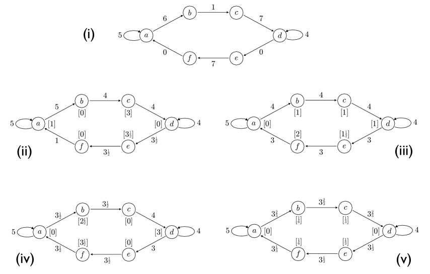
Figure 2. Example showing convergence of raising and lowering operations. (i) A graph function $\alpha$. (ii) The raising-balanced graph function $\alpha^{R}$ obtained in the limit from $\alpha$ by raising operations; numbers in square brackets at the vertices show the limiting raising vector $r^{*}$. (iii) The balanced graph function $(\alpha^{R})^{L}$ obtained in the limit by applying lowering operations to $\alpha^{R}$, together with its associated lowering vector. (This is the unique balanced graph function to which the two-phase algorithm “converges” if both phases are run to convergence.) Figures (iv) and (v) show the graph functions $\alpha^{L}$ and $(\alpha^{L})^{R}$ respectively (and their associated lowering/raising vectors), obtained by reversing the order of the raising and lowering phases. Note that the balanced graph functions $(\alpha^{R})^{L}$ (in (iii)) and $(\alpha^{L})^{R}$ (in (v)) are not the same; while both versions (raising-lowering and lowering-raising) converge to a unique balanced graph function, these limits are not equal. The graph function $\alpha$ is not UB.

5. Rate of convergence

In this section we will prove the main result of the paper, Theorem 3 from the Introduction, which gives a tight bound on the rate of convergence of the iterative balancing algorithm. We restate the result here for convenience.

Theorem 3. On input $(A,\varepsilon)$, where $A$ is an arbitrary irreducible non-negative matrix with imbalance $\rho$, the above two-phase $L_{\infty}$ balancing algorithm performs $O(n^{3}\log(n\rho/\varepsilon))$ balancing operations and outputs a matrix equivalent to $A$ that is $\varepsilon$-balanced w.h.p.

We give here a brief, high-level outline of our analysis. First note that, by Proposition 4 in the previous section, it suffices to analyze each phase of the algorithm separately. Accordingly, we will analyze only the raising phase, showing that it achieves an $\varepsilon$-raising-balanced graph function w.h.p. after $O(n^{3}\log(\rho/\varepsilon))$ raising operations. By symmetry the same bound holds for the lowering phase: simply observe that lowering on the graph $G_{\alpha}$ is equivalent to raising on the transpose graph $G^{T}_{\alpha}$.

In the Introduction we already discussed some of the difficulties which prevent us from analyzing the dynamics of the algorithm by tracking a scalar quantity at each vertex, as would be the case for the analogous but much simpler heat-kernel dynamics. A key ingredient in our solution to the problem is to introduce a two-dimensional representation of the graph function $\alpha$, together with an associated potential function that will enable our analysis of the raising phase. One coordinate (the vertical coordinate) in this representation, called the “height” of a vertex, is based on the unique raising vector $r^{*}$ whose existence is guaranteed by Lemma 7 of the previous section; the second (horizontal) coordinate is the “level” of the vertex, as alluded to in the Introduction. This representation, which is specified in detail in Section 5.1, will be instrumental in obtaining upper and lower bounds relating the (global) potential function to the local imbalances (which govern the effect of a single raising operation); these bounds are derived in Sections 5.2 and 5.3 respectively. Finally, in Section 5.4 we conclude the proof of Theorem 3.

5.1. A two-dimensional representation

Throughout this and the next two subsections, we focus exclusively on the raising phase. As we observed above, exactly the same rate of convergence will apply to the lowering phase.

Recall from Lemma 7 that, for any initial graph function $\alpha$, the limiting raising vector $r^{*}$, which records the asymptotic total amount of raising performed at each vertex by any infinite fair sequence of raising operations, is uniquely defined and specifies a unique raising balanced graph function $\alpha^{R}$. We may therefore use $r^{*}$ to define a height function

$${y}_{v}:=-r^{*}_{v},$$

i.e., $-{y}_{v}$ is the amount of raising that remains to be performed at vertex $v$ in order to reach the raising-balanced graph function $\alpha^{R}$. (Note that, throughout, all heights are non-positive and converge monotonically to zero. This convention turns out to be convenient in our analysis.) The heights are related to $\alpha$ and $\alpha^{R}$ by

(3) $$\alpha^{R}_{uv}-\alpha_{uv}={y}_{u}-{y}_{v},$$

which is just a restatement of equation (1).

In addition to the heights ${y}_{v}$, we will need to introduce a second coordinate ${x}_{v}$ defined by

(4) $$x_{v}:=\max_{u:u\to v}\alpha^{R}_{uv}.$$

We refer to ${x}_{v}$ as the level of vertex $v$. Note that (intuitively at least), lower level vertices can only reliably be close to raising-balanced after higher level ones are close, so the levels capture one of the distinguishing features of the problem. The two-dimensional representation $(x_{v},{y}_{v})$ of vertices $v$ will be key to the remainder of our argument.

Figure 3 shows the two-dimensional representation of the graph function in Figure 2(i). The horizontal coordinates can be read off from the maximum incoming edges at each vertex in Figure 2(ii), and the vertical coordinates from the square brackets in the same figure.

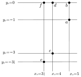
Figure 3. Two-dimensional representation of the graph function $\alpha$ shown in Figure 2(i).

We will measure progress of the raising phase by means of the global potential function $\Psi=-\sum{y}_{v}$, which is the total amount of raising that remains to be done to reach $\alpha^{R}$. In order to relate $\Psi$ to the local imbalances $\rho_{v}^{R}$, it will be convenient to introduce a closely related global quantity $h$, which is just the difference between the maximum and minimum heights. That is, setting ${y}_{\min}=\min_{u}{y}_{u}$ and ${y}_{\max}=\max_{u}{y}_{u}$, we define

$$h:={y}_{\max}-{y}_{\min}.$$

(As we shall see shortly (Corollary 11), it is always the case that ${y}_{\max}=0$ so in fact $h=-{y}_{\min}$.) Note that $\Psi$ and $h$ differ by at most a factor of $n$, namely:

(5) $$\Psi\geq h\geq\frac{1}{n}\Psi.$$

The key ingredients in our analysis are the following two bounds relating $h$ to the local imbalances $\rho_{v}^{R}$.

Proposition 8.

For any graph function $\alpha$, we have $\rho^{R}/2\leq h$.

Proposition 9.

For any graph function $\alpha$, we have $h\leq(n-1)\sum_{v}\rho^{R}_{v}$.

Proposition 8 confirms that, to ensure $\varepsilon$-raising-balance, it suffices to achieve $\Psi\leq\varepsilon/2$. The much more subtle Proposition 9 implies that $\Psi$ decreases at each step by an expected $(1-\Omega(\frac{1}{n^{3}}))$ factor. To see this implication, note that the expected decrease in $\Psi$ in one raising operation is $\frac{1}{2n}\sum_{v}\rho_{v}^{R}$, and apply Proposition 9 and equation (5).

In the next two subsections we prove Propositions 8 and 9 respectively.

5.2. Proof of Proposition 8

The proposition will follow almost immediately from the following straightforward lemma relating heights to local imbalances. Since we are dealing exclusively with the raising phase, in this and the next two subsections we will write $\rho_{v},\rho$ in place of $\rho_{v}^{R},\rho^{R}$ to simplify notation.

Lemma 10.

Let $\alpha$ be a graph function and $v$ a vertex with $\rho_{v}>0$. Then there exist edges $(u,v)$ and $(v,w)$ in $G_{\alpha}$ such that

(6) $${y}_{v}+\frac{\rho_{v}}{2}\leq\frac{{y}_{u}+{y}_{w}}{2}.$$

Proof.

Let $u,w$ be vertices such that $\alpha_{uv}=\alpha^{\text{in}}_{v}$ and $\alpha_{vw}=\alpha^{\text{out}}_{v}$ (i.e., $(u,v)$ and $(v,w)$ are incoming and outgoing edges of maximum weight at $v$). Note that $\rho_{v}=\alpha_{vw}-\alpha_{uv}$.

To prove (6) we let $u^{\prime}$ be a vertex such that the edge $(u^{\prime},v)$ achieves the maximum in (4), i.e., $\alpha^{R}_{u^{\prime}v}=x_{v}$, and write

(7) $${y}_{v}+\frac{\rho_{v}}{2} = {y}_{u^{\prime}}+\alpha_{u^{\prime}v}-\alpha^{R}_{u^{\prime}v}+\frac{\rho_{v}}{2}$$

$$= {y}_{u^{\prime}}+\alpha_{u^{\prime}v}-\alpha^{R}_{u^{\prime}v}+\frac{\alpha_{vw}-\alpha_{uv}}{2}$$

$$\leq {y}_{u^{\prime}}-\alpha^{R}_{u^{\prime}v}+\frac{\alpha_{vw}+\alpha_{u^{\prime}v}}{2},$$

where in the first line we used equation (3) and in the last line the fact that $\alpha_{u^{\prime}v}\leq\alpha_{uv}$. Now two further applications of equation (3) give

$$\alpha_{vw} = {y}_{w}-{y}_{v}+\alpha^{R}_{vw};$$

$$\alpha_{u^{\prime}v} = {y}_{v}-{y}_{u^{\prime}}+\alpha^{R}_{u^{\prime}v}.$$

Plugging these into (7) yields

$${y}_{v}+\frac{\rho_{v}}{2}\leq{y}_{u^{\prime}}-\alpha^{R}_{u^{\prime}v}+\frac{{y}_{w}-{y}_{u^{\prime}}+\alpha^{R}_{vw}+\alpha^{R}_{u^{\prime}v}}{2}=\frac{{y}_{u^{\prime}}+{y}_{w}}{2}+\frac{\alpha^{R}_{vw}-\alpha^{R}_{u^{\prime}v}}{2}\leq\frac{{y}_{u^{\prime}}+{y}_{w}}{2},$$

where the last inequality follows from the facts that $\alpha^{R}$ is raising balanced and $\alpha^{R}_{u^{\prime}v}$ is maximal among incoming edges at $u$. This completes the proof.    $\Box$

Before proving Proposition 8, we pause to observe a consequence of Lemma 10:

Corollary 11.

$y_{\max}=0$.

Proof.

A raising operation applied at some vertex $v$ increases $y_{v}$ to ${y}_{v}+\frac{\rho_{v}}{2}$. By Lemma 10 this is $\leq\frac{{y}_{u}+{y}_{w}}{2}\leq y_{\max}$. Therefore $y_{\max}$ can never increase during the raising phase. Choose a vertex $u$ so that $y_{u}=y_{\max}$ initially. Then $u$ can never rise, and so $r^{*}_{u}=0$. Thus $y_{\max}=y_{u}=-r^{*}_{u}=0$.    $\Box$

We conclude this subsection by proving Proposition 8.

Proof of Proposition 8. Let $v$ be any vertex with raising imbalance $\rho_{v}>0$. By Lemma 10 we have

$$\frac{\rho_{v}}{2}\leq\frac{{y}_{u}+{y}_{w}}{2}-{y}_{v}\leq y_{\max}-y_{\min}=h.$$

Together with the fact that, by definition, $h\geq 0$, this completes the proof.    $\Box$

5.3. Proof of Proposition 9

The reverse inequality, Proposition 9, is considerably more delicate. It will make crucial use of the two-dimensional representation introduced earlier, as well as one additional concept which we call “momentum,” whose role will emerge shortly. The momentum of a vertex $v$ is defined by

(8) $$m_{v}:=\max_{u:u\to v}\{\alpha_{uv}-{x}_{v}\},$$

where ${x}_{v}$ is the level of $v$ as defined above.

One key property of momentum is that it can be upper bounded at a vertex in terms of the sum of the momentum and the local imbalance at the predecessors of the vertex in the graph. (The form of this bound is complicated by a dependence on the levels of the vertices; see part (i) of Lemma 12.) The second key property of momentum is that, along any edge, height can increase only at a rate bounded by momentum and local imbalance. (Again there are additional terms complicating the dependence; see part (ii) of Lemma 12.) Putting these two properties together will show that, if the height difference between some two vertices in the graph is substantial, then the aggregate local imbalance $\textstyle\sum_{v}\rho_{v}$ must be large, which is exactly the content of Proposition 9.

Lemma 12.

The momentum satisfies the following inequalities:

• For any vertex $v$,   $m_{v}\leq\max\big{\{}0,\max_{u:u\to v,{y}_{u}<{y}_{v}}(m_{u}+\rho_{u}+{x}_{u}-{x}_{v})\big{\}}$.

• For any edge $(u,v)$ in $G_{\alpha}$,   ${y}_{v}\leq{y}_{u}+m_{u}+\rho_{u}+{x}_{u}-\alpha^{R}_{uv}$.

Proof.

Both parts rely on the following elementary observation. For any edge $(u,v)$, by the definition of $\rho_{u}$ we have

(9) $$\alpha_{uv}\leq\max_{u^{\prime}:u^{\prime}\to u}\alpha_{u^{\prime}u}+\rho_{u}=m_{u}+\rho_{u}+{x}_{u},$$

where we have used the definition of momentum (8).

For part (i), we thus have

$$m_{v}=\max_{u:u\to v}\{\alpha_{uv}-{x}_{v}\}\leq\max_{u:u\to v}\{m_{u}+\rho_{u}+{x}_{u}-{x}_{v}\}.$$

Now note that if ${y}_{u}\geq{y}_{v}$ we have, recalling equations (3, 4),

(10) $$\alpha_{uv}-{x}_{v}={y}_{v}-{y}_{u}+\alpha^{R}_{uv}-{x}_{v}\leq 0.$$

This justifies the restriction on the right-hand side of (i) to maximization over $u$ s.t. ${y}_{u}<{y}_{v}$. This completes the proof of (i).

For part (ii), apply equations (3, 9) to deduce

$${y}_{v}={y}_{u}+\alpha_{uv}-\alpha^{R}_{uv}\leq{y}_{u}+m_{u}+\rho_{u}+{x}_{u}-\alpha^{R}_{uv},$$

as required.    $\Box$

To complete the proof of Proposition 9, we need to translate Lemma 12, which gives local bounds on the increase of momentum and height between adjacent vertices, into global bounds in $G_{\alpha}$, as specified in Lemma 13 below. The key to this translation will be to apply part (ii) of Lemma 12 to a carefully chosen sequence of edges, for each of which the extra term $x_{u}-\alpha^{R}_{uv}$ in the lemma is non-positive and which together span the heights in the graph; these edges will be identified in Lemma 14 below.

For a vertex $v$, let $S_{v}$ denote the set of vertices whose height is strictly smaller than $v$, i.e., $S_{v}=\{u:{y}_{u}<{y}_{v}\}$. Also, let $\rho(S_{v})=\sum_{u\in S_{v}}\rho_{u}$. Finally, define

(11) $$z_{v}:=\max\{{x}_{u}:{y}_{u}\leq{y}_{v}\}-{x}_{v}.$$

This definition has the consequences that $z_{v}\geq 0$ and

(12) $$[y_{u}\leq y_{v}]\Rightarrow[x_{u}+z_{u}\leq x_{v}+z_{v}].$$

We are now ready to state our global bounds.

Lemma 13.

For any vertex $v$, the following two bounds hold:

1. $m_{v}\leq\rho(S_{v})+{z}_{v}$;

2. ${y}_{v}-y_{\min}\leq|S_{v}|\cdot\rho(S_{v})$.

Proof.

Both parts (i) and (ii) are proved by induction on vertices $v$ in order of height. We begin with part (i), which will be used in the proof of part (ii).

Part (i). We use induction on the height ${y}_{v}$ of $v$. If ${y}_{v}=\min_{u}y_{u}$, the statement is true since $m_{v}\leq 0$ (this follows from part (i) of Lemma 12) and the right-hand side is non-negative. Assuming ${y}_{v}>\min_{u}y_{u}$, and beginning with part (i) of Lemma 12, we may write

$$m_{v} \leq \max\big{\{}0,\max_{u:u\to v,{y}_{u}<{y}_{v}}\{m_{u}+\rho_{u}+{x}_{u}-{x}_{v}\}\big{\}}$$

$$\leq \max\big{\{}0,\max_{u:u\to v,{y}_{u}<{y}_{v}}\{\rho(S_{u})+{z}_{u}+\rho_{u}+{x}_{u}-{x}_{v}\}\big{\}}$$

$$\leq \max\big{\{}0,\max_{u:u\to v,{y}_{u}<{y}_{v}}\{\rho(S_{v})+{z}_{u}+{x}_{u}-{x}_{v}\}\big{\}},$$

where in the second line we applied induction to bound $m_{u}$ since ${y}_{u}<{y}_{v}$, and in the third line we used the fact that $u\in S_{v}\setminus S_{u}$ to deduce that $\rho(S_{u})+\rho_{u}\leq\rho(S_{v})$.

To complete the proof we need only apply Eqn. (12) to conclude that for all $u$ in the last maximization, $x_{u}+z_{u}\leq x_{v}+z_{v}$.

Part (ii). Again we use induction on the height of $v$. The base case is ${y}_{v}=y_{\min}$, in which case the statement holds trivially.

Now let $v$ be any vertex with $y_{\min}<{y}_{v}$, and suppose part (ii) is established for all $u$ with $y_{u}<{y}_{v}$. Let $U$ be the subset of $\{u:y_{u}<y_{v}\}$ having $x_{u}=x_{U}$, where $x_{U}=\max\{x_{u}:y_{u}<y_{v}\}$. Of course $U\neq\emptyset$, and $z_{u}=0$ for all $u\in U$. We require the following additional fact:

Lemma 14.

There is a vertex $u^{\prime}\in U$ having an edge $(u^{\prime},v^{\prime})$ where $v^{\prime}\notin U$, $\alpha^{R}_{u^{\prime}v^{\prime}}\geq x_{U}$, $y_{v^{\prime}}\geq y_{v}$.

We defer the proof of Lemma 14 to the end of the subsection and continue with the proof of Lemma 13(ii). Applying part (ii) of Lemma 12 to the edge $(u^{\prime},v^{\prime})$ provided by Lemma 14, we have

$${y}_{v}\,\leq\,{y}_{v^{\prime}} \leq {y}_{u^{\prime}}+m_{u^{\prime}}+\rho_{u^{\prime}}+{x}_{u^{\prime}}-\alpha^{R}_{u^{\prime}v^{\prime}}$$

$$\leq {y}_{u^{\prime}}+m_{u^{\prime}}+\rho_{u^{\prime}}$$

$$\leq {y}_{u^{\prime}}+\rho(S_{u^{\prime}})+{z}_{u^{\prime}}+\rho_{u^{\prime}}$$

$$= {y}_{u^{\prime}}+\rho(S_{u^{\prime}})+\rho_{u^{\prime}}$$

$$\leq y_{\min}+|S_{u^{\prime}}|\rho(S_{u^{\prime}})+\rho(S_{u^{\prime}})+\rho_{u^{\prime}}$$

$$\leq y_{\min}+|S_{v}|\rho(S_{v}).$$

In the second line here we have used the guarantee of Lemma 14 that $\alpha^{R}_{u^{\prime}v^{\prime}}\geq x_{U}$; in the third line we have used part (i) of the current lemma; in the fourth line we have used the fact noted earlier that $z_{u^{\prime}}=0$ for any $u^{\prime}\in U$; in the fifth line we have used the inductive hypothesis applied to ${y}_{u^{\prime}}$ (which is strictly less than ${y}_{v}$); and in the last line we have used the fact that $u^{\prime}\in S_{v}\setminus S_{u^{\prime}}$. This completes the inductive proof of part (ii) of the lemma.    $\Box$

Our main goal in this subsection, Proposition 9, now follows trivially from Lemma 13.

Proof of Proposition 9. By part (ii) of Lemma 13 we have, for any vertex $v$, ${y}_{v}-{y}_{\min}\leq(n-1)\sum_{u}\rho_{u}$.    $\Box$

It remains only for us to supply the missing proof of Lemma 14.

Proof of Lemma 14. The proof will follow from two claims.

Claim (i): Every vertex $u\in U$ has an outgoing edge $(u,w)$ with $\alpha^{R}_{uw}=x_{U}$.

To state the second claim, define the graph $G^{\prime}$ formed by the set of edges $\{(u,w):u\in U,\alpha^{R}_{uw}\geq x_{U}\}$.

Claim (ii): There is an edge $(u,w)\in G^{\prime}$ such that $w\notin U$.

Claim (ii) implies the lemma because $(u,w)\in G^{\prime}$ implies $\alpha^{R}_{uw}\geq x_{U}$; this last implies also that $x_{w}\geq x_{U}$; and then $w$ cannot have $y_{w}<y_{v}$ as it would then be in $U$.

Proof of Claim (i): Since $u\in U$, we know that ${y}_{u}<0$ and hence some raising must eventually be performed at $u$, i.e., eventually $\rho^{R}_{u}>0$ and then $\rho^{L}_{u}=0$. But once this happens, the same argument as in the proof of Proposition 4 shows that $\rho^{L}_{u}=0$ at all future times, and hence in $\alpha^{R}$ (at the conclusion of the raising phase) we must have $\rho^{R}_{u}=\rho^{L}_{u}=0$. Thus if $(u,w)$ is a maximum outgoing edge at $u$ in $\alpha^{R}$, we have $\alpha^{R}_{uw}=\max_{v}\alpha^{R}_{vu}=x_{U}$.    $\Box$

Proof of Claim (ii): By Claim (i), every $u\in U$ has an outgoing edge in $G^{\prime}$. Suppose for contradiction that $w\in U$ for all edges of $G^{\prime}$. Then in $G^{\prime}$ there is a sink scc on vertices $U^{\prime}\subseteq U$. ($U^{\prime}$ may be as small as a single vertex with a self-loop.)

Let $\delta_{0}=-\max_{u^{\prime}\in U^{\prime}}{y}_{u^{\prime}}$. Note that $\delta_{0}>0$. Also, let $\delta_{1}=\min\{\alpha^{R}_{rr^{\prime}}-\alpha^{R}_{ss^{\prime}}:\alpha^{R}_{rr^{\prime}}-\alpha^{R}_{ss^{\prime}}>0\}$; if this set is empty let $\delta_{1}=\infty$. Finally, select $0<\delta<\min\{\delta_{0},\delta_{1}\}$.

Now fix any infinite fair sequence of raising operations, and consider the first operation in the sequence that increases any ${y}_{u}$, $u\in U^{\prime}$, to a value larger than $-\delta$. (This is well defined as all ${y}_{u},u\in U^{\prime}$ increase monotonically to zero.) Let $u^{\prime}$ be the vertex raised by this operation, and let $\alpha$ be the graph function immediately after the operation and ${y}$ the height function corresponding to $\alpha$.

By construction there is an edge $(t,u^{\prime})$ in $G^{\prime}$, with $t\in U^{\prime}$. Applying equation (3) to the edge $(t,u^{\prime})$, we see that

(13) $$\alpha_{tu^{\prime}}=\alpha^{R}_{tu^{\prime}}+y_{u^{\prime}}-y_{t}\geq x_{U}+y_{u^{\prime}}-y_{t}\geq x_{U},$$

where the first inequality is because the edge is in $G^{\prime}$, and the second inequality is by choice of $u^{\prime}$. (Note that equality can hold here only if $t=u^{\prime}$.)

Now let $(u^{\prime},w)$ be a maximum (in $\alpha$) outgoing edge at $u^{\prime}$. Since a nontrivial raising operation has just been performed at $u^{\prime}$, it must be the case that $w\neq u^{\prime}$. (Raising preserves the order of weights among outgoing edges in $\alpha$. If a self-loop is a maximal outgoing edge from $u^{\prime}$ in $\alpha$ then it was also maximal before raising. But then there could have been no nontrivial raising at $u^{\prime}$.) Also, since we have just raised at $u^{\prime}$, $\rho^{L}_{u^{\prime}}=0$, so $\alpha_{u^{\prime}w}\geq\alpha_{tu^{\prime}}$. Combining with (13) we have

(14) $$\alpha_{u^{\prime}w}\geq x_{U}.$$

Applying equation (3) to the edge $(u^{\prime},w)$ we get

$$\alpha^{R}_{u^{\prime}w}=\alpha_{u^{\prime}w}+{y}_{u^{\prime}}-{y}_{w}\geq\alpha_{u^{\prime}w}+{y}_{u^{\prime}}\geq\alpha_{u^{\prime}w}-\delta\geq x_{U}-\delta,$$

where the first inequality is because heights are nonpositive, the second is by the choice of $u^{\prime}$, and the third is by equation (14). But since $\delta<\delta_{1}$ this in fact implies that $\alpha^{R}_{u^{\prime}w}\geq x_{U}$. Hence the edge $(u^{\prime},w)$ belongs to $G^{\prime}$, and since $U^{\prime}$ is a sink scc it must be the case that $w\in U^{\prime}$. But this implies that $\alpha^{R}_{u^{\prime}w}\leq x_{w}=x_{U}$, and therefore in fact that $\alpha^{R}_{u^{\prime}w}={x}_{U}$; and also, by choice of $u^{\prime}$, that ${y}_{w}<{y}_{u^{\prime}}$. Hence

$$\alpha_{u^{\prime}w}=\alpha^{R}_{u^{\prime}w}-{y}_{u^{\prime}}+{y}_{w}=x_{U}-{y}_{u^{\prime}}+{y}_{w}<x_{U},$$

which in light of (14) gives us the desired contradiction. This completes the proof of Claim (ii) and therefore the lemma.    $\Box$

5.4. Proof of Theorem 3

We are now finally in a position to prove our main result, Theorem 3.

Proof of Theorem 3. It suffices to show that, with high probability, $O(n^{3}\log(\rho n/\varepsilon))$ raising operations suffice to achieve an $\varepsilon$-raising-balanced graph function. As we observed at the beginning of the section, by symmetry the same holds for the lowering phase, and hence the output of the algorithm will be $\varepsilon$-balanced w.h.p.

To analyze the raising phase, we index all quantities by $t$, the number of raising operations that have so far been performed. Thus in particular ${y}_{v}(t)$ is the height of vertex $v$ after $t$ raising operations. We also introduce the potential function $\Psi(t)=-\sum_{v}{y}_{v}(t)$. Note that $\Psi(t)\geq 0$ and that $\Psi(t)$ decreases monotonically to 0 as $t\to\infty$. Moreover, by Proposition 8 we have

$$\Psi(t)=-\sum_{v}{y}_{v}(t)\geq h(t)\geq\rho^{R}(t)/2.$$

Hence in order to achieve raising imbalance at most $\varepsilon$ after $t$ raising steps it suffices to ensure that $\Psi(t)\leq\varepsilon/2$.

Since a raising operation at vertex $v$ increases ${y}_{v}$ by $\rho^{R}_{v}/2$, the expected decrease in $\Psi(t)$ in one raising operation is

$${\rm E}[\Psi(t)-\Psi(t+1)]=\frac{1}{2n}\sum_{v}\rho^{R}_{v}(t)\geq\frac{h(t)}{2n(n-1)}=\frac{-{y}_{\min}(t)}{2n(n-1)}\geq\frac{1}{2n^{3}}\Psi(t),$$

where in the first inequality we have used Proposition 9, in the next step Corollary 11, and in the last inequality the fact that ${y}_{\min}$ is less than the average of the ${y}_{v}$. Iterating for $t$ steps yields

$${\rm E}[\Psi(t)]\leq\Bigl{(}1-\frac{1}{2n^{3}}\Bigr{)}^{t}\Psi(0).$$

To get an upper bound on $\Psi(0)$, we observe that

$$\Psi(0)=-\sum_{v}{y}_{v}(0)\leq-n{y}_{\min}(0)=nh(0)\leq n(n-1)\sum_{v}\rho^{R}_{v}(0)\leq n^{3}\rho^{R}(0)\leq n^{3}\rho,$$

where we have again used Corollary 11 and Proposition 9. (Recall that $\rho=\max\{\rho^{R}(0),\rho^{L}(0)\}$ is the imbalance of the original matrix.) Hence, for any $\delta\in(0,1)$, after $t=6n^{3}\ln(2\rho n/\varepsilon\delta)$ raising operations we have

$${\rm E}[\Psi(t)]\leq\varepsilon\delta/2.$$

By Markov’s inequality this implies that $\Psi(t)\leq\varepsilon/2$ with probability at least $1-\delta$. To obtain the result w.h.p., it suffices to take $\delta=o(1)$.    $\Box$

6. Open problems

We close the paper with some remarks and open problems.

1.  The introduction of raising and lowering phases into the Osborne-Parlett-Reinsch algorithm is trivial from an implementation perspective (the effect being simply to censor some of the balancing operations), but seemingly crucial to our analysis. If balancing operations of both types are interleaved, we no longer have a reliable measure of progress. It would be interesting to modify the analysis so as to handle an arbitrary sequence of balancing operations, and on the other hand to investigate whether the introduction of phases actually improves the rate of convergence (both in theory and in practice). Similarly, it would be interesting to investigate the effect of choosing a random sequence of indices at which to perform balancing, rather than a deterministic sequence as in the original algorithm.

2.  Recall that, without raising and lowering phases, the balanced matrix to which the algorithm converges is not unique (except, by definition, in the UB case). It would be interesting to investigate the geometric structure of the set of fixed points, which apparently can be rather complicated.

3.  As we have seen, our $\widetilde{O}(n^{3})$ bound on the worst case convergence time is essentially optimal. While this goes some way towards explaining the excellent performance of the algorithm in practice, more work needs to be done to explain its empirical dominance over algorithms with faster worst-case asymptotic running times. In particular, can one identify features of “typical” matrices that lead to much faster convergence?

4.  We have analyzed only the $L_{\infty}$ variant of the Osborne-Parlett-Reinsch algorithm. It would be interesting to analyze the algorithm for other norms $L_{p}$, in particular $L_{2}$ and $L_{1}$. (In the latter case, the problem corresponds to finding a circulation—in the sense of network flows—that is equivalent to the initial assignment of flows to the edges of the graph.)

7. Acknowledgements

We thank Tzu-Yi Chen and Jim Demmel for introducing us to this problem and for several helpful pointers, Martin Dyer for useful discussions, and Yuval Rabani for help in the early stages of this work which led to the proof of Theorem 1. We also thank anonymous referees of an earlier version for suggestions that improved the presentation of the paper.

Appendix A Proof of convergence

In this section we present an alternative proof of convergence of the original Osborne-Parlett-Reinsch $L_{\infty}$ balancing algorithm. As remarked earlier this was first proved by Chen [2] using a compactness argument. In the interests of making the present paper self-contained, we give here an alternative proof that is more combinatorial in nature. For this proof only, we explicitly allow more general sequences of balancing operations, subject only to the “fairness” constraint that every index $i$ appears infinitely often. (Clearly, the random sequence discussed in the main text has this property with probability 1.) Note, however, that this proof does not apply to the two-phase version of the algorithm which we analyze in this paper because the sequence of balancing operations in that version is not fair. We prove convergence of the two-phase version in Section 4.

Theorem 15.

Consider the Osborne-Parlett-Reinsch $L_{\infty}$ balancing algorithm applied to any irreducible (real or complex) input matrix $A$, and assume that balancing operations are performed infinitely often at all indices $i$. Then the algorithm converges, i.e., if $A^{(t)}$ is the sequence of matrices after each step of the algorithm, then there exists a balanced matrix $B$ equivalent to $A$ such that $A^{(t)}\to B$ as $t\to\infty$.

Proof. We work in the framework of Section 2, representing $A$ as a graph $G_{\alpha}$ with an associated graph function $\alpha$, where $\alpha_{uv}=\log|a_{uv}|$ (and edges $(u,v)$ with $a_{uv}=0$ are omitted). We let $\alpha_{v}^{\text{in}}$ and $\alpha_{v}^{\text{out}}$ denote the maximum incoming and outgoing edge weights at vertex $v$ in $G_{\alpha}$; we also set $\alpha_{v}^{\text{max}}=\max\{\alpha_{v}^{\text{in}},\alpha_{v}^{\text{out}}\}$.

The key ingredient in the proof is the following partial order on graph functions defined on a common strongly-connected graph $G$. For two such graph functions $\alpha,\gamma$, we say that $\alpha<\gamma$ if, for the largest weight $w$ such that $G_{\alpha}^{w}\neq G_{\gamma}^{w}$, we have $G_{\alpha}^{w}\subset G_{\gamma}^{w}$.

Now, if a decreasing sequence $\alpha^{(t)}$ of graph functions in this order has the property that all values $\alpha^{(t)}_{uv}$ in the functions are bounded below by a common value $b$, it is clear that the sequence has a limit. The convergence of the iterative balancing algorithm will therefore follow from the next two lemmas. Call a balancing operation at $i$ non-trivial if $\alpha_{v}^{\text{in}}\neq\alpha_{v}^{\text{out}}$, so that the operation actually changes the weights. By definition $\alpha$ is balanced iff no non-trivial balancing operation is available.

Lemma 16.

Non-trivial balancing operations are strictly decreasing in the above order on graph functions.

Proof.

Let $\alpha$ be the current graph function, and let $v$ be a vertex at which a non-trivial balancing operation is performed. Let $\bar{\alpha}$ denote the new graph function after the operation. We have $\bar{\alpha}_{v}^{\text{max}}=\alpha_{v}^{\text{max}}-|\bar{\alpha}_{v}^{\text{in}}-\bar{\alpha}_{v}^{\text{out}}|/2$, and $\bar{\alpha}_{v}^{\text{max}}<\alpha_{v}^{\text{max}}$. The balancing operation affects only edges incident at $v$. Before the balancing, at least one of those edges belongs to $G_{\alpha}^{\alpha_{v}^{\text{max}}}$, while none belong to $G_{\alpha}^{w}$ for any $w>\alpha_{v}^{\text{max}}$. After the balancing, none of those edges belong to $G_{\alpha}^{\alpha_{v}^{\text{max}}}$. Thus the largest value of $w$ for which $G_{\alpha}^{w}$ and $G_{\bar{\alpha}}^{w}$ differ is $w=\alpha_{v}^{\text{max}}$, and $G_{\bar{\alpha}}^{\alpha_{v}^{\text{max}}}\subset G_{\alpha}^{\alpha_{v}^{\text{max}}}$.    $\Box$

Lemma 17.

Given any graph function $\alpha$, there is a $b>-\infty$ such that no sequence of balancing operations can create an edge of weight less than $b$.

Proof.

A balancing operation at vertex $v$ reduces $\alpha_{v}^{\text{max}}$, so no such operation can increase the maximum edge value above its original value in $G_{\alpha}$, say $m_{1}$. Let $w_{1}$ be the least average weight of any cycle in $G_{\alpha}$; note that $w_{1}$ remains invariant under any sequence of balancing operations. Consider the value of any edge $(u,v)$ under any graph function $\alpha^{\prime}$ that is reached by balancing operations from $\alpha$. Let $(u,v)$ belong to some (simple) cycle of average weight $w_{2}$ and length $\ell$. Then $(\alpha^{\prime}_{uv}+(\ell-1)m_{1})/\ell\geq w_{2}\geq w_{1}$, so $\alpha^{\prime}_{uv}\geq w_{1}-(\ell-1)(m_{1}-w_{1})\geq w_{1}-(n-1)(m_{1}-w_{1})$. This completes the proof of the lemma and the theorem.    $\Box$

References

- [1] S. Boyd, L. El Ghaoui, E. Feron, and V. Balakrishnan. Linear Matrix Inequalities in System and Control Theory. SIAM Studies in Applied Mathematics Vol. 15, 1994.
- [2] T.-Y. Chen. Balancing sparse matrices for computing eigenvalues. Master’s thesis, UC Berkeley, May 1998.
- [3] T.-Y. Chen and J. Demmel. Balancing sparse matrices for computing eigenvalues. Linear Algebra and its Applications, 309:261–287, 2000.
- [4] B. C. Eaves, A. J. Hoffman, U. G. Rothblum, and H. Schneider. Line-sum-symmetric scalings of square non-negative matrices. Math. Programm. Study, 25:124–141, 1985.
- [5] J. Franklin and J. Lorenz. On the scaling of multidimensional matrices. Linear and Multilinear Algebra, 23:717–735, 1989.
- [6] J. Grad. Matrix balancing. The Computer Journal, 14:280–284, 1971.
- [7] D. J. Hartfiel. Concerning diagonal similarity of irreducible matrices. Proceedings of the American Mathematical Society, 30:419–425, 1971.
- [8] B. Kalantari and L. Khachiyan. On the rate of convergence of deterministic and randomized RAS matrix scaling algorithms. Operations Research Letters, 14:237–244, 1993.
- [9] B. Kalantari and L. Khachiyan. On the complexity of nonnegative matrix scaling. Linear Algebra and its Applications, 240:87–104, 1996.
- [10] B. Kalantari, L. Khachiyan, and A. Shokoufandeh. On the complexity of matrix balancing. SIAM Journal on Matrix Analysis and Applications, 18:450–463, 1997.
- [11] B. Kalantari, I. Lari, F. Ricca, and B. Simeone. On the complexity of general matrix scaling and entropy minimization via the RAS algorithm. Mathematical Programming, 112(2):371–401, 2008.
- [12] D. Kressner. Numerical Methods for General and Structured Eigenvalue Problems. Springer, 2005.
- [13] N. Linial, A. Samorodnitsky, and A. Wigderson. A deterministic strongly polynomial algorithm for matrix scaling and approximate permanents. Combinatorica, 20:531–544, 2000.
- [14] E. E. Osborne. On pre-conditioning of matrices. Journal of the ACM, 7(4):338–345, 1960.
- [15] B. N. Parlett and C. Reinsch. Balancing a matrix for calculation of eigenvalues and eigenvectors. Numerische Mathematik, 13:293–304, 1969.
- [16] H. Schneider and M. H. Schneider. Max-balancing weighted directed graphs and matrix scaling. Mathematics of Operations Research, 16(1):208–222, 1991.
- [17] L. J. Schulman and A. Sinclair. Analysis of a classical matrix preconditioning algorithm. Proceedings of the 47th Annual ACM Symposium on Theory of Computing (STOC), 2015.
- [18] R. Sinkhorn. A relationship between arbitrary positive matrices and doubly stochastic matrices. Annals of Mathematical Statistics, 35:876–879, 1979.
- [19] T. Ström. Minimization of norms and logarithmic norms by diagonal similarities. Computing, 10:1–7, 1972.
- [20] L. N. Trefethen and M. Embree. Spectra and Pseudospectra: The Behavior of Nonnormal Matrices and Operators. Princeton University Press, 2005.
- [21] N. Young, R. E. Tarjan, and J. B. Orlin. Faster parametric shortest path and minimum balance algorithms. Networks, 21:205–221, 1991.