Solution of the Hyperon Puzzle within a Relativistic Mean-Field Model

Abstract

The equation of state of cold baryonic matter is studied within a relativistic mean-field model with hadron masses and coupling constants depending on the scalar field. All hadron masses undergo a universal scaling, whereas the couplings are scaled differently. The appearance of hyperons in dense neutron star interiors is accounted for, however the equation of state remains sufficiently stiff if the reduction of the $\phi$ meson mass is included. Our equation of state matches well the constraints known from analyses of the astrophysical data and particle production in heavy-ion collisions.

, and

1 Introduction

A nuclear equation of state (EoS) is one of the key ingredients in the description of neutron star (NS) properties [1], supernova explosions [2] and heavy-ion collisions [3, 4]. A comparison of various EoSs in how well they satisfy various empirical constraints was undertaken in Ref. [5] for the EoSs obtained within relativistic mean-field models (RMF) and some more microscopic calculations and in Ref. [6] for the Skyrme models. It turns out difficult to reconcile the constraint on the maximum NS mass, which must be larger than $1.97\,M_{\odot}$ after the recent measurements reported in [7, 8], and the upper constraints on the stiffness of the EoS extracted from the analyses of heavy-ion collisions (HICs) [3, 4]. Another relevant constraint on the EoS of the NS matter is imposed by the direct Urca (DU) processes, like $n\to p+e+\bar{\nu}$, which occur as soon as the nucleon density exceeds some critical value $n_{\rm DU}^{n}$. The occurrence of these very efficient processes, even with account for the nucleon pairing, is hardly compatible with NS cooling data, if the value of the NS mass, at which the central density becomes larger than $n_{\rm DU}^{n}$, is $M_{\rm DU}^{n}<1.5M_{\odot}$ (the so-called “strong” DU constraint) [9, 5]. There should be $M_{\rm DU}^{n}<1.35M_{\odot}$ (the “weak” DU constraint) [10, 5], since $1.35\,M_{\odot}$ is the mean value of the NS mass distribution, as it follows from the analysis of the observational data on NSs in binary systems. The DU problem appears in the EoSs with linear dependence of the symmetry energy except, maybe, most stiff ones. All the standard RMF EoSs and the microscopic Dirac-Brueckner-Hartree-Fock (DBHF) EoS suffer of this linear dependence. On the contrary, variational calculations of the Urbana-Argonne group with A18 + $\delta v$ + UIX* forces [11], as well as the RMF models with density dependent hadron coupling constants [12], generate a weaker growth of the symmetry energy with the density, and the problem with the DU reactions is avoided. The later models are also able to describe NSs, as heavy as those in Refs. [7, 8].

The problems worsen if strangeness is taken into account, because the population of new Fermi seas of hyperons leads to a softening of the EoS and reduction of the maximum NS mass. By employing a recently constructed hyperon-nucleon potential, the maximum masses of NSs with hyperons are computed to be well below $1.4M_{\odot}$ [13]. Also, within RMF models one is able to explain observed massive NSs only, if one artificially prevents the appearance of hyperons, cf. [13, 14] and the references therein. This is called in the literature, the “hyperon puzzle”. So, the difference between NS masses with and without hyperons proves to be so large for reasonable hyperon fractions in the standard RMF approach that in order to solve the puzzle one has to start with very stiff purely nuclear EoS, that hardly agrees with the results of the microscopically-based variational EoS [11] and the EoS calculated with the help of the auxiliary field diffusion Monte Carlo method [15]. Such an EoS would also be incompatible with the restrictions on the EoS stiffness extracted from the analysis of nucleon and kaon flows in heavy-ion collisions [3, 4]. All suggested explanations require additional assumptions, see discussion in [16]. For example, the inclusion of an interaction with a $\phi$-meson mean field, and the usage of smaller ratiohypreon-nucleon coupling constants following the SU(3) symmetry relations [17], as well as other modifications performed within the standard RMF approach, all help to increase the NS mass.

There is also another part of the “hyperon puzzle”, which attracted less attention so far. With the hyperon coupling constants introduced with the help of the SU(6) symmetry relations the critical densities for the appearance of first hyperons prove to be rather low, $n_{\rm DU}^{H}\sim 3n_{0}$, cf. [18, 19]. However with the appearance of the hyperons the efficient DU reaction on hyperons, e.g. $\Lambda\to p+e+\bar{\nu}$, occurs that may potentially cause a very rapid cooling of the NSs with $M>M_{\rm DU}^{H}$, $M_{\rm DU}^{H}$ being the NS mass, at which the central density reaches the value $n^{H}_{\rm DU}$. The problem should be additionally studied with account for a suppression of hyperon concentrations and weak interaction vertices of hyperons compared to the corresponding neutron concentrations and nucleon weak interaction vertices, and with account for the hyperon pairing, cf. [20, 21].

In Ref. [10] two of us formulated an RMF model, in which hadron masses and meson-baryon coupling constants are dependent on the $\sigma$ mean field. A working model MW(n.u., z=0.65) labeled in [5] as KVOR model has been constructed. This model was shown in [5] to satisfy appropriately the majority of experimental constraints known by that time. In Ref. [22] the particle thermal excitations were incorporated and the model was successfully applied to description of heavy-ion collisions. However hyperons are not included in the model. Even without hyperons the KVOR EoS with the added (BPS) crust EoS from [23] yields $M_{\rm max}^{\rm KVOR}=2.01M_{\odot}$ that fits the new constraint [7, 8] only marginally.

In the present Letter we will show that within the RMF models with hadron masses and coupling constants dependent on the $\sigma$ mean field one is able to overcome the mentioned above problems and to construct the appropriate EoS with hyperons satisfying presently known experimental constraints.

2 Energy density functional

In our RMF model we include nucleons $N=(p,n)$ and hyperons $H=(\Lambda^{0},\Sigma^{\pm,0},\Xi^{-,0})$ interacting with mean fields of mesons $m=\sigma,\omega,\rho,\phi$. For simplicity, we drop the $\rho$ meson self-interaction and disregard, therefore, a possibility of the charged $\rho$-meson condensation discussed in [10]. As the bare masses of the particles we take $m_{N}=938$ MeV, $m_{\Lambda}=1116$ MeV, $m_{\Sigma}=1193$ MeV, $m_{\Xi}=1318$ MeV and neglect the small mass splitting in isospin multiplets. Lepton masses are $m_{e}=0.5$ MeV and $m_{\mu}=105$ MeV.

Following the approach [10], the scalar field enters as a dimensionless variable $f=g_{\sigma N}\chi_{\sigma N}(\sigma)\sigma/m_{N}$ and the meson-baryon coupling constants $g_{mB}$, $B=(N,H)$, are made $\sigma$-dependent with the help of scaling coupling constants, $g_{mB}\chi_{mB}(f)$ with $\chi_{\omega H}(f)=\chi_{\omega N}(f)$ , $\chi_{\rho H}(f)=\chi_{\rho N}(f)$ . The bare masses of hadrons $m_{B}$ and $m_{m}$ are replaced in the model by the effective masses $m_{B}^{*}=m_{B}\Phi_{B}(f)$ and $m_{m}^{*}=m_{m}\Phi_{m}(f)$ scaled by the functions

$$\Phi_{N}(f) =\Phi_{m}(f)=1-f\,,$$

$$\Phi_{H}(f) =1-x_{\sigma H}\frac{m_{N}}{m_{H}}\xi_{\sigma H}f\,,$$ (1)

where $x_{\sigma H}={g_{\sigma H}}/{g_{\sigma N}}$ and $\xi_{\sigma H}(f)=\chi_{\sigma H}(f)/\chi_{\sigma N}(f)$.

Taking into account the equations of motion for vector fields, the energy density of the cold infinite matter with an arbitrary isospin composition is recovered from the Lagrangian of the model in the standard way, see Ref. [10]:

$$E[f]=\sum_{B}E_{\rm kin}\big{(}p_{{\rm F},B},m_{B}\Phi_{B}(f)\big{)}+\sum_{l=e,\mu}E_{\rm kin}(p_{{\rm F},l},m_{l})$$

$$\,\,+\frac{m_{N}^{4}f^{2}}{2C_{\sigma}^{2}}\eta_{\sigma}(f)+\frac{1}{2m_{N}^{2}}\Big{[}\frac{C_{\omega}^{2}\widetilde{n}_{B}^{2}}{\eta_{\omega}(f)}+\frac{C_{\rho}^{2}\widetilde{n}_{I}^{2}}{\eta_{\rho}(f)}+\frac{C_{\phi}^{2}\widetilde{n}_{S}^{2}}{\eta_{\phi}(f)}\Big{]}\,,$$ (2)

$$\widetilde{n}_{B}=\sum_{B}x_{\omega B}n_{B}\,,\,\widetilde{n}_{I}=\sum_{B}x_{\rho B}t_{3B}n_{B}\,,\,\widetilde{n}_{S}=\sum_{H}x_{\phi H}n_{H}\,,$$

where $x_{\omega(\rho)B}=g_{\omega(\rho)B}/g_{\omega(\rho)N}$, $x_{\phi H}=g_{\phi H}/g_{\omega N}$, $g_{\phi N}=0$.

The values of the isospin projections for baryons $t_{3i}$ follow from the Gell-Mann–Nishijima relation $t_{3B}=Q_{B}-(1+S_{B})/2$, where $Q_{B}$ and $S_{B}$ are the baryon electric charge and strangeness, respectively. The baryon densities are related to the baryon Fermi momentum as $n_{B}=p_{{\rm F},B}^{3}/3\pi^{2}$ and the fermionic kinetic energy density is

$$E_{\rm kin}(p_{\rm F},m)=\int_{0}^{p_{\rm F}}\frac{p^{2}dp}{\pi^{2}}\sqrt{p^{2}+m^{2}}\,.$$

The dimensionless coupling constants are $C_{m}=\frac{g_{mN}m_{N}}{m_{m}}$ for all $m$ except $\phi$. Since the ratios $x_{\phi H}$ are determined through $g_{\omega N}$, the $\phi$-field contribution enters the energy density with the constant $C_{\phi}=C_{\omega}m_{\omega}/m_{\phi}$. Here we take $m_{\omega}=783\,{\rm MeV}$, $m_{\phi}=1020\,{\rm MeV}$. Bare masses and coupling constants of all mesons except $\phi$ enter the energy density only in combinations $C_{m}$ and the scaling functions $\Phi_{m}$ and $\chi_{m}$ enter only through the scaling factors

$$\eta_{m}(f)=\Phi_{m}^{2}(f)/\chi_{mN}^{2}(f)\,.$$ (3)

Therefore we actually do not need to determine $\Phi_{m}(f)$ and $\chi_{m}(f)$ separately, but only $\eta_{m}(f)$ combinations. The self-interaction of the scalar field introduced usually in RMF models through a potential $U(f)$ is hidden now in the definition of $\eta_{\sigma}(f)$. The equation of motion for the remaining field variable $f$ follows from the minimization of the energy density $\partial E[f]/\partial f=0\,.$ If we suppress $\phi$ and $H$ terms, put $\eta_{\sigma}=1+2\frac{C_{\sigma}^{2}}{f^{2}}(\frac{b}{3}f^{3}+\frac{c}{4}f^{4})$ and put all other scaling functions to unity, we recover the energy density functional of the standard non-linear Walecka $\sigma$-$\omega$-$\rho$ model.

For the NS matter sustained in the $\beta$-equilibrium the Fermi momenta of a baryon can be expressed through the baryon chemical potential, $\mu_{B}$, as $p_{{\rm F},B}^{2}=(\mu_{B}-V_{B})^{2}-m^{2}_{B}\Phi^{2}_{B}$, where $V_{B}\,m_{N}^{2}=C^{2}_{\omega}x_{\omega B}\tilde{n}_{B}/\eta_{\omega}+C^{2}_{\rho}x_{\rho B}t_{3B}\tilde{n}_{I}/\eta_{\rho}+C^{2}_{\phi}x_{\phi B}\tilde{n}_{S}/\eta_{\phi}$; $\mu_{B}$ is related to the nucleon and electron chemical potentials as $\mu_{B}=\mu_{n}-Q_{B}\mu_{e}$. Solving the system of equations for $p_{{\rm F},B}$ and making use of the electro-neutrality condition $\sum_{B}Q_{B}n_{B}=n_{e}+n_{\mu}$, where the lepton densities are $n_{e}=\mu_{e}^{3}/3\pi^{2}$, $n_{\mu}=(\mu_{e}^{2}-m_{\mu}^{2})^{3/2}/3\pi^{2}$, we can express the hadron densities and the total energy density through the total baryon density $n=\sum_{B}n_{B}$. The total pressure is calculated as $P=\sum_{i=B,l}\mu_{i}n_{i}-E$.

The parameters of the nucleon sector are tuned to reproduce the properties of nuclear matter at saturation: the saturation density $n_{0}$, the binding energy per nucleon $\mathcal{E}_{0}$, the effective nucleon mass $m_{N}^{*}$, the compressibility modulus $K$ and the symmetry energy $\widetilde{J}$. The coupling constants of hyperons with vector mesons are interrelated by SU(6) symmetry relations [26]:

$$g_{\omega\Lambda}=g_{\omega\Sigma}=2g_{\omega\Xi}={\textstyle\frac{2}{3}}g_{\omega N}\,,\,\,\,g_{\rho\Sigma}=2g_{\rho\Xi}=2g_{\rho N}\,,$$

$$2g_{\phi\Lambda}=2g_{\phi\Sigma}=g_{\phi\Xi}=-{\textstyle\frac{2\sqrt{2}}{3}}g_{\omega N}\,,\quad g_{\rho\Lambda}=g_{\phi N}=0\,.$$ (4)

The coupling constants of hyperons with the scalar mean field are constrained with the help of the hyperon binding energies per nucleon $\mathcal{E}_{\rm bind}^{H}$ in the isospin symmetric matter (ISM) at $n=n_{0}$ given by [18]:

$$\mathcal{E}_{\rm bind}^{H}(n_{0}) =C_{\omega}^{2}m_{N}^{-2}x_{\omega H}n_{0}-(m_{N}-m_{N}^{*}(n_{0}))x_{\sigma H}\,,$$ (5)

where we suppose $\xi_{\sigma H}(f(n_{0}))=1$ and use

$$\mathcal{E}_{\rm bind}^{\Lambda}(n_{0})=-28\,{\rm MeV},\quad\mathcal{E}_{\rm bind}^{\Sigma}(n_{0})=30\,{\rm MeV},$$

$$\mathcal{E}_{\rm bind}^{\Xi}(n_{0})=-15\,{\rm MeV}\,.$$ (6)

The repulsive $\Sigma$ potential prevents the appearance of $\Sigma$ hyperons in all models considered below.

The NS configuration follows from the solution of the Tolman–Oppenheimer–Volkoff equation. For $n\stackrel{{\scriptstyle\scriptstyle<}}{{\phantom{}{}_{\sim}}}(0.6-0.8)n_{0}$, our RMF EoSs should be matched with the EoS of the NS crust, where the formation of a pasta phase is explicitly included. The presence of the pasta, although it may change transport properties of the matter, affects an EoS only slightly  [24]. Therefore simplifying consideration we chose the frequently-used crust BPS EoS from [23], ignoring the pasta phase. The same BPS crust EoS was used in [5] where it was joined with the various EoSs describing the interior region. The pressure as a function of the density for the EoSs, we consider here, intersects the BPS pressure at density $n_{1}$, such that $0.45n_{0}\stackrel{{\scriptstyle\scriptstyle<}}{{\phantom{}{}_{\sim}}}n_{1}\stackrel{{\scriptstyle\scriptstyle<}}{{\phantom{}{}_{\sim}}}0.7n_{0}$. We construct the resulting pressure as a function of the density by using the BPS pressure for $n\leq 0.45n_{0}$, then a cubic spline interpolation for $0.45n_{0}<n\leq 0.7n_{0}$, and the pressure for beta-equilibrium matter (BEM) given by our model for $n>0.7\,n_{0}$. The choice of the interval, which includes the intersection points for both EoSs, guarantees the smoothness of the interpolation. We have also checked that a narrowing of the interpolation interval limits almost does not reflect on such observables as the star mass and radius.

3 Models

We discuss now two models constructed according to the principles described above. One is the formal extension of the KVOR model from Ref. [10] to hyperons, which we call the KVORH model now. In this example we demonstrate the problems, which appear when one includes hyperons. For the second model, labeled as MKVOR (or MKVORH when hyperons are included), we propose new set of scaling functions. In Table 1 we present the saturation parameters for both models and the coefficients of the expansion of the nucleon binding energy per nucleon near the nuclear saturation density $n_{0}$,

$$\mathcal{E}=\mathcal{E}_{0}+\frac{K}{2}\epsilon^{2}-\frac{K^{{}^{\prime}}}{6}\epsilon^{3}+\beta^{2}\widetilde{J}(n)+O(\beta^{4})\,,$$

$$\widetilde{J}(n)=\widetilde{J}+L\epsilon+\frac{K_{\rm sym}}{2}\epsilon^{2}+\dots\,,$$ (7)

in terms of small $\epsilon=(n-n_{0})/3n_{0}$ and $\beta=(n_{n}-n_{p})/n$ parameters.

Table 1: Characteristics of KVOR and MKVOR models at saturation

EoS	$\mathcal{E}_{0}$	$n_{0}$	$K$	$m_{N}^{*}(n_{0})$	$\widetilde{J}$	$L$	$K^{\prime}$	$K_{\rm sym}$
	[MeV]	[fm-3]	[MeV]	$[m_{N}]$	[MeV]	[MeV]	[MeV]	[MeV]
KVOR	$-16$	0.16	275	0.805	32	71	422	-86
MKVOR	$-16$	0.16	240	0.73	30	41	557	-158

3.1 KVORH model

Reference [10] proposed a set of input parameters for the RMF model, which matches the APR EoS (in the relativistic HHJ parameterization of [27]) up to $n\stackrel{{\scriptstyle\scriptstyle<}}{{\phantom{}{}_{\sim}}}4n_{0}$, see Eq. (61) in [10]. To fulfill the DU constraint Ref. [10] introduced the scaling function $\eta_{\rho}(f)\neq 1$, see Eq. (63) in [10]. Thus the model labeled as KVR in Ref. [5] was constructed. The idea behind the KVOR modification of the KVR model was to demonstrate that introducing the additional scaling function $\eta_{\omega}\neq 1$ one can increase the maximum value of the NS mass without a sizable change of the EoS for densities $n\stackrel{{\scriptstyle\scriptstyle<}}{{\phantom{}{}_{\sim}}}4n_{0}$. The coupling constants for the KVOR model are given in Eq. (58) in Ref. [10]. The KVOR model produces the maximum NS mass $M_{\rm max}=2.01M_{\odot}$, and the critical proton density for the DU reaction threshold on neutrons $n_{\rm DU}^{n}=3.92n_{0}$ corresponding to $M_{\rm DU}^{n}=1.76M_{\odot}$.

In the KVORH model the parameters $x_{\sigma H}$ deduced from hyperon binding energies in Eq. (5) are

$$x_{\sigma\Lambda}=0.599\,,\,\,\,x_{\sigma\Sigma}=0.282\,,\,\,\,x_{\sigma\Xi}=0.305\,.$$ (8)

The baryon concentrations for the KVORH model are depicted in Fig. 1 as functions of the baryon density $n$. For $n<0.6n_{0}$ the curves presented in Fig. 1 should be replaced by those computed within the EoS of the crust. The KVORH model produces the maximum NS mass $M_{\rm max}=1.66M_{\odot}$. The critical density for the appearance of first hyperons, which is simultaneously the critical density for the onset of the DU reactions on hyperons ($\Lambda$ in this case) is $n_{\rm DU}^{\Lambda}=2.82n_{0}$, and the corresponding NS mass at which first $\Lambda$s appear in the NS center is $M_{\rm DU}^{\Lambda}=1.38M_{\odot}$. The total strangeness concentration (the ratio of the number of strange quarks to the total number of quarks) in the NS with the maximum mass is $f_{\rm S}=0.034$ .

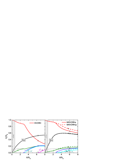
Figure 1: Baryon concentrations and the variable $f$ in BEM as functions of total baryon density for the KVORH, MKVORH$\phi$ and MKVORH$\phi\sigma$ models. Dotted lines show the thresholds of the DU reaction on neutrons. For the MKVORH$\phi$ and MKVORH$\phi\sigma$ models the thresholds are not distinguishable on the plot scale. Short vertical bars on the lines show the maximum densities reachable in the NS for the given model.

3.2 MKVORH model

Reference [10] showed that the EoS is more sensitive to the value of $m_{N}^{*}(n_{0})$ than to the compressibility $K$. The smaller $m_{N}^{*}(n_{0})$ is in a certain RMF model, the larger is the value of the maximum NS mass. The input parameters for the new MKVOR model are listed in Table 1 together with the corresponding parameters of the nuclear binding energy per nucleon at saturation. We took in the MKVOR model a smaller value of $m_{N}^{*}(n_{0})$ than in the KVOR model and a smaller value of the compressibility, $K=240$ MeV, that agrees with canonical value $K=240\pm 20$ MeV extracted from the analysis of giant monopole resonances (GMR) [28].

The scaling functions of the MKVOR model are as follows:

$$\eta_{\sigma}^{-1}(f)=1-\frac{2}{3}C_{\sigma}^{2}bf\big{[}1+\frac{3}{4}\big{(}c-\frac{8}{9}C_{\sigma}^{2}b^{2}\big{)}f\big{]}+\frac{1}{3}df^{3}\,,$$

$$\eta_{\omega}(f)=\Big{(}\frac{1+zf_{0}}{1+zf}\Big{)}^{\alpha}+\frac{a_{\omega}}{2}\left[1+\tanh(b_{\omega}(f-f_{\omega}))\right]\,,$$

$$\eta_{\rho}(f)=a_{\rho}^{(0)}+a_{\rho}^{(1)}f+\frac{a_{\rho}^{(2)}f^{2}}{1+a_{\rho}^{(3)}f^{2}}$$

$$\quad\quad\,\,+\beta\exp\Big{[}-\gamma\frac{(f-f_{\rho})^{2}({1+e_{\rho}(f-f_{0})^{2}})}{1+d_{\rho}(f-f_{0})+e_{\rho}(f-f_{0})^{2}}\Big{]}\,.$$ (9)

The parameters of the model and of the scaling functions are collected in Table 2. The choice of the scaling functions is definitively not unique. Their final form was tuned to satisfy best the experimental constraints, that we demonstrate below, and to keep a connection to the KVOR model parameterization. The first term in $\eta_{\omega}$ is the same as in the KVOR model, the function $\eta_{\sigma}$ and the first three terms in $\eta_{\rho}$ are basically the reparameterization of the functions of the KVOR model. The new terms, the second one in $\eta_{\omega}$ and the last one in $\eta_{\rho}$ are added to control the growth of the scalar field with density. Note that the density dependencies of our scaling functions for the $\sigma N$, $\omega N$ and $\rho N$ coupling constants prove to be similar to those exploited in the DD and DD-F models with the density dependent coupling constants and bare meson field masses, cf. [25, 5].

Table 2: Parameters of the MKVOR model

$C_{\sigma}^{2}$		$C_{\omega}^{2}$		$C_{\rho}^{2}$	$b\cdot 10^{3}$	$c\cdot 10^{3}$	$d$	$\alpha$	$z$	$a_{\omega}$
234.15		134.88		81.842	4.6750	$-2.9742$	$-0.5$	0.4	0.65	0.11
$b_{\omega}$	$f_{\omega}$	$\beta$	$\gamma$	$f_{\rho}$	$a_{\rho}$	$a_{\rho}^{(1)}$	$a_{\rho}^{(2)}$	$a_{\rho}^{(3)}$	$d_{\rho}$	$e_{\rho}$
7.1	0.9	3.11	28.4	0.522	0.448	$-0.614$	3	0.8	$-4$	6

The maximum NS mass increases in the MKVOR model compared to the KVOR model up to $M_{\rm max}=2.33\,M_{\odot}$. The DU threshold values are $n_{\rm DU}^{n}=4.14n_{0}$ and $M_{\rm DU}^{n}=2.22M_{\odot}$.

In the model with hyperons (MKVORH) we use the $\sigma H$ coupling constant ratios deduced from hyperon binding energies in ISM following Eq. (5) for $\xi_{\sigma H}=1$:

$$x_{\sigma\Lambda}=0.607\,,\,\,\,x_{\sigma\Sigma}=0.378\,,\,\,\,x_{\sigma\Xi}=0.307\,.$$ (10)

Note that the value $x_{\sigma\Lambda}\simeq 0.61$ is close to the best value derived from hypernuclei $x_{\sigma\Lambda}\simeq 0.62$ in Ref. [26].

To have an opportunity for an increase of the maximum NS mass in the model with hyperons, we incorporate the $\phi$-meson mean field with a scaled $\phi$ meson mass (version labeled MKVORH$\phi$) and, additionally, allow for a scaling of the $\sigma H$ coupling constants, $\xi_{\sigma H}(n)\neq 1$ (version MKVORH$\phi\sigma$).

In the model MKVORH$\phi$ we will exploit the very same scaling of the $\phi$-meson mass as for other hadrons $\Phi_{\phi}=1-f$. This implies the scaling function

$$\eta_{\phi}=(1-f)^{2}\,.$$ (11)

We use the minimal model, assuming parameterization Eq. (4) for the vector-meson–hyperon coupling constants, and the $\sigma H$ coupling constants from Eq. (10). As the result the maximum NS mass in MKVORH$\phi$ model becomes $M_{\rm max}=2.22\,M_{\odot}$ with the strangeness concentration $f_{\rm S}=0.023$. The critical density for the appearance of first hyperons is $n_{\rm DU}^{\Lambda}=2.63n_{0}$, corresponding to the star mass $M_{\rm DU}^{\Lambda}=1.43\,M_{\odot}$. Although the model does not satisfy the “strong” DU constraint ($M_{\rm DU}>1.5M_{\odot}$), we should notice that for reactions on hyperons this constraint might be a bit soften since the baryon part of the squared matrix element of the DU reaction on $\Lambda$s is 25 times smaller than that for the DU reaction on neutrons [20], besides the pairing gaps might be not as small.

The effect of the $\xi_{\sigma H}(n)$ scaling we demonstrate at hand of the MKVORH$\phi\sigma$ model, where we take $\xi_{\sigma H}(n)$ such that $\xi_{\sigma H}(n\leq n_{0})=1$, and assume that $\xi_{\sigma H}(n)$ decreases with an increase of $n$ and vanishes for densities $n>\min\{n_{\rm DU}^{H}\}$. This means that effectively we will exploit vacuum hyperon masses for $n>\min\{n_{\rm DU}^{H}\}$. Note that the KVOR model extended to high temperatures in Ref. [22] (called there as the SHMC model) matches well the lattice data up to $T\sim 250$ MeV provided $\sigma B$ coupling constants for all baryons except the nucleons, are artificially suppressed, that partially motivates our choice of suppressed values $\xi_{\sigma H}$.

The baryon concentrations from the MKVORH$\phi$ and MKVORH$\phi\sigma$ models are shown in Fig. 1. The proton fractions of the MKVORH$\phi$ and MKVORH$\phi\sigma$ models are smaller than those for the KVORH model. We also see that inclusion of the $\phi$ scaling (11) reduced the hyperon population. The reduction of the $\sigma H$ coupling constants prevents the appearance of $\Lambda$ and $\Xi^{0}$ hyperons and shifts the threshold density of the $\Xi^{-}$ appearance to higher values. Without $\Lambda$s the reaction $\Xi^{-}\to\Lambda+e^{-}+\bar{\nu}_{e}$ does not occur and the DU threshold is determined by the DU reactions on nucleons. Replacing the values of $f(n)$ depicted in Fig. 1 for the BEM in Eq. (1) one can recover the density dependence of the effective hadron masses and from Eqs. (9) and (11) that of the effective coupling constants. Within the MKVORH$\phi\sigma$ model we get $M_{\rm max}=2.29\,M_{\odot}$, $n_{\rm DU}^{n}=3.69\,n_{0}$ ($M_{\rm DU}^{n}=2.09\,M_{\odot}$), and the total strangeness concentration in the heaviest NS is reduced to $f_{\rm S}=6.2\times 10^{-3}$.

Applying the $\phi$-mass scaling and the $\xi_{\sigma H}$ scaling to the KVORH model we obtain for the KVORH$\phi$ model $M_{\rm max}=1.88\,M_{\odot}$ and that the first hyperons, $\Lambda$s, appear at the density $n_{\rm DU}^{\Lambda}=2.81\,n_{0}$ ($M_{\rm DU}^{\Lambda}=1.37\,M_{\odot}$). The strangeness fraction is $f_{\rm S}=0.035$. For the KVORH$\phi\sigma$ model we find $M_{\rm max}=1.96\,M_{\odot}$, $f_{\rm S}=9.2\times 10^{-3}$. The first among hyperons appear $\Xi^{-}$s, therefore the DU threshold is shifted to $n_{\rm DU}^{n}=3.95\,n_{0}$ ($M_{\rm DU}^{n}=1.76\,M_{\odot}$).

Below we compare how well the EoSs obtained within the MKVORH$\phi\sigma$ and KVORH models satisfy various phenomenological constraints.

4 Constraints on the models

4.1 Symmetry energy and nucleon optical potential

Figure 2: (Left) The symmetry energy coefficient $\widetilde{J}(n)$ as a function of the nucleon density calculated in the KVOR and MKVOR models. Shaded area shows the constraint from the study of analog isobar states (AIS) in [29]. Hatched area is the constraint from the electric dipole polarizability $(\alpha_{\rm D})$ in ²⁰⁸Pb [30]. (Right) The nucleon optical potential as a function of the nucleon kinetic energy for ISM at $n=n_{0}$ for the KVOR, cf. [22], and MKVOR models. Shaded area shows the extrapolation from finite nuclei to the nuclear matter from [32].

Constraints on the density dependence of the symmetry energy [parameter $\tilde{J}(n)$ in Eq. (7)] are extracted in [29] from the study of the analog isobar states and in [30] from the electric dipole polarizability of ²⁰⁸Pb nuclei. They are shown in Fig. 2 (left panel) by the shaded and hatched regions, respectively, together with the symmetry energies calculated in the KVOR and MKVOR models. We see that the both models follow the lower boundary of the region.

The dependence of the nucleon optical potential on the nucleon kinetic energy in the ISM at $n=n_{0}$ is shown in Fig. 2 (right panel). The shaded region is extracted from the atomic nucleus data [31] and recalculated to the case of the infinite nuclear ISM in [32]. The KVOR model describes the nucleon optical potential for low and high particle energies but does not describe it for intermediate energies. The MKVOR model describes the nucleon optical potential rather well for nucleon energies $E_{N}-m_{N}\stackrel{{\scriptstyle\scriptstyle<}}{{\phantom{}{}_{\sim}}}400$ MeV. To fit appropriately the data at higher particle energies, the momentum dependence of the $NN$ interaction would be required that is not present in the mean-field approach. The iso-vector part of the optical potential $U_{\rm opt}^{n}-U_{\rm opt}^{p}$ is less constrained by the data, therefore we do not show it.

4.2 Particle flow in heavy-ion collisions

The analysis of the transverse and elliptical flow data in HICs allowed [3] to extract a constraint on the pressure of the ISM as a function of the nucleon density and to reconstruct the pressure for the purely neutron matter (PNM) with some assumptions about the density dependence of the symmetry energy $\tilde{J}(n)$ (soft or stiff one). Reference [33] on the basis of calculations of the kaon production in HICs  [4] provided some restrictions on the pressure at lower densities. These constraints are shown in Fig. 3 together with the results of the GMR data analysis taken from [33] and the pressure calculated in the KVOR and MKVOR models. The constraints rule out a very stiff EoS. We see that the KVOR model satisfies the requirements. The MKVOR model fulfills the constraints, for $n<4n_{0}$ in ISM. For PNM the MKVOR curve passes through the hatched region with stiffer $\tilde{J}(n)$, whereas the KVOR EoS is softer. The choice of the smaller $m_{N}^{*}(n_{0})$ leads to a stiffening of the EoS in ISM and the scaling functions $\eta_{\sigma}(f)$ and $\eta_{\omega}(f)$ are chosen to soften the EoS for $n\stackrel{{\scriptstyle\scriptstyle<}}{{\phantom{}{}_{\sim}}}4n_{0}$ to fulfill the nucleon- and kaon-flow constraints. To increase the maximum NS mass we had to stiffen the EoS in the BEM that was accomplished by the choice of the $\eta_{\rho}$ function.

Figure 3: Pressure as a function of the nucleon density in ISM and PNM for the KVOR and MKVOR models. Hatched areas show the empirical constraints from the analyses of a particle flow in HICs in [3], kaon production in HICs [33, 4], and the GMR data [33].

4.3 DU constraint

In the BEM the DU process on neutrons, $n\to p+e+\bar{\nu}_{e}$, can occur only, if the proton fraction is high enough so that the Fermi momenta of neutrons, protons and electrons ($p_{{\rm F},i=n,p,e}$) satisfy the inequality $p_{{\rm F},n}\leq p_{{\rm F},p}+p_{{\rm F},e}$. Usually, RMF models yield uncomfortably low values of the threshold densities for these reactions and correspondingly low values of the NS mass, $M_{\rm DU}^{n}$, at which the process begins to occur in the NS center. Every star with a mass only slightly above $M_{\rm DU}^{n}$ cools down fast due to the DU process, even in the presence of nucleon pairing, and becomes invisible for the thermal detection within few years [9]. Most of single NSs have likely masses below $1.5M_{\odot}$ in accordance with the type-II supernova explosion scenario [2] and the population synthesis analysis [34]. Therefore, it is natural to believe that majority of the pulsars, which surface temperatures have been measured, have masses $M\stackrel{{\scriptstyle\scriptstyle<}}{{\phantom{}{}_{\sim}}}1.5M_{\odot}$. The analysis of these data in the existing cooling scenarios supports the constraint $M_{\rm DU}^{n}\stackrel{{\scriptstyle\scriptstyle>}}{{\phantom{}{}_{\sim}}}1.5M_{\odot}$ [35, 36]. The adequate description of the new data on the cooling of the Cassiopea A also requires the absence of the DU reactions [35].

In the presence of $\Lambda$ hyperons, reactions $\Lambda\to p+e+\bar{\nu}$ may occur. As seen in Fig. 1, proton concentrations for the KVORH, MKVORH$\phi$ models do not exceed the neutron-DU threshold for $n<n_{\rm DU}^{\Lambda}$, and for higher densities the DU reactions on $\Lambda$s start occurring. For the MKVORH$\phi\sigma$ model $\Lambda$s do not appear at all and the DU processes occur for $n>n_{\rm DU}^{n}$.

4.4 Gravitational mass versus baryon mass constraint

The unique double-neutron-star system J0737-3039 with two millisecond pulsars provided an important constraint on the nuclear EoS. The gravitational mass of one of the companions (B) is very low $M_{G}=1.249\pm 0.001M_{\odot}$ [37] which implies a very peculiar mechanism of its creation – a type-I supernova of an O-Ne-Mg white dwarf driven hydrostatically unstable by electron captures onto Mg and Ne. Knowing this mechanism Refs. [38, 39] calculated the number of baryons in the pulsar and the corresponding baryon mass: $M_{B}=1.366\mbox{--}1.375M_{\odot}$ [38] and $M_{B}=1.358\mbox{--}1.362$ [39]. The constraint of Ref. [38] can be released by $1\%\,M_{\odot}$ because of a possible baryon loss and a critical mass variation due to carbon flashes during the collapse. Therefore one can speak about “strong” (without the mass loss) and “weak” (with the mass loss) constraints on the EoS, respectively. Microscopically motivated EoSs, like the relativistic DBHF EoS [41], the APR EoS [11], the diffusion Monte-Carlo one [15], and many RMF-based models do not fulfill the strong constraint of Ref. [38]. Many EoSs do not satisfy the constraint of  [39] and even the weak constraint of Ref. [38], cf. [5].

Figure 4: (Left) Gravitational NS mass $M_{G}$ versus the baryon mass $M_{B}$. Shaded rectangles show the constraints from J0737-3039(B) pulsar derived in Refs. [38] and [39] labeled by 1 and 2, respectively. The empty rectangle demonstrates the change of the constraint [38] by 1% $M_{\odot}$. (Right) The NS mass-radius relations for the KVORH, MKVORH$\phi$, MKVORH$\phi\sigma$ models compared with constraints from the isolated NS RX J1856.5 3754 [40], QPOs in the LMXBs 4U 0614+09 [42], the millisecond pulsar PSR J0437-4715 [43], and the Bayesian probability distribution analyses (BPA) [1]. The horizontal lines border the uncertainty range for the mass of PSR J0348+0432 [8].

In Fig. 4 (left panel) we plot the gravitational NS mass $M_{G}$ versus the baryon mass $M_{B}$. The KVOR model matches marginally the weak constraint of Ref. [38], whereas the MKVOR model matches marginally both the result from Ref. [39] and the strong constraint of  [38], the latter was not reproduced by the EoSs considered in Ref. [5]. Note that hyperons do not appear in the NS with the mass of $1.25M_{\odot}$, therefore the curves for the models KVORH and KVOR coincide, as well as the curves for the MKVOR, MKVORH$\phi$ and MKVORH$\phi\sigma$ models. Comparing particle concentration for different models shown in Fig. 1 and the baryon mass of the NS, we observe a correlation: the smaller is the proton fraction within the density interval $n_{0}<n\stackrel{{\scriptstyle\scriptstyle<}}{{\phantom{}{}_{\sim}}}2.5n_{0}$, the better the given EoS satisfies the baryon-mass constraint. For $n\sim n_{0}$ the value of the proton fraction is correlated with the values of $\widetilde{J}$ and $L$ in Eq. (7). The value of $\widetilde{J}$ may vary only a little (from 28 MeV to 34 MeV or even in a narrower interval) but $L$ varies broadly in various works, e.g., cf. Fig. 4 in Ref. [33]. With a decrease of $L$ curves in Fig. 4 (left panel) are shifted to the right. For $L<40$ MeV (at fixed other parameters) the MKVOR curves would pass through the shaded area 1. The smaller $L$ is for the given EoS, the less the proton fraction is in the relevant density interval $n_{0}<n\stackrel{{\scriptstyle\scriptstyle<}}{{\phantom{}{}_{\sim}}}2.5n_{0}$, and the better the constraint is satisfied.

4.5 Mass and radius constraints

In Fig. 4 (right panel) we show mass-radius relations of NSs for the KVORH, MKVORH$\phi$ and MKVORH$\phi\sigma$ models. Largest precisely-measured masses of NSs are $1.97\pm 0.04M_{\odot}$ for PSR J1614-2230 [7] and $2.01\pm 0.04M_{\odot}$ for PSR J0348+0432 [8]. The MKVORH$\phi$ and MKVORH$\phi\sigma$ models can describe these high-mass NSs, whereas the KVORH model fails badly. Experimental information about heavier NSs is plagued with large experimental errors and with additional theoretical uncertainties, see Ref. [1] for a review. In Fig. 4 (right panel) we confront our models with other constraints derived from the quasi-periodic oscillations in the low-mass X-ray binary 4U 0614+091 [42] and thermal spectra of the nearby isolated NS RX J1856.5-3754 [40]. More details on these constraints can be found in Ref. [5]. In contrast to the mass determination, there are no accurate estimates of NS radii. Some constraints were derived recently from the X-ray spectroscopy of PSR J0437 4715 with the proper account for the system geometry [43] and from the Bayesian probability analysis of several X-ray burst sources in Ref. [1]. These constraints are also shown in Fig. 4. We see that the MKVORH$\phi$ and MKVORH$\phi\sigma$ satisfy the mass-radius constraints and produce the radii of NSs in a narrow interval $11.7\pm 0.5$ km for star masses $M>0.5M_{\odot}$.

5 Concluding remarks

We constructed relativistic mean-field models with scaled hadron masses and coupling constants including a $\phi$ meson mean field and hyperons. The hyperon–vector–meson ($\omega,\rho,\phi$) coupling constants obey the SU(6) symmetry relations. The most challenging is to fulfill the flow constraint and produce a high maximum neutron-star mass simultaneously. For that we introduced the scaling functions such that our equation of state is rather soft for $n\stackrel{{\scriptstyle\scriptstyle<}}{{\phantom{}{}_{\sim}}}4n_{0}$ in the isospin symmetric matter but is sufficiently stiff in the beta-equilibrium matter. This behavior is achieved by the proper selection of the scaling functions $\eta_{\omega}$ and $\eta_{\rho}$. The inclusion of the $\phi$ meson with the mass scaled in the same way as masses of nucleons and other mesons, but with the $\phi$ coupling constants being fixed, allows to fulfill the empirical constraints on the maximum neutron star mass; see curve for the MKVORH$\phi$ model in Fig. 4 (right panel). In such an approach the “hyperon puzzle” can be resolved within our model without any additional assumptions, like, e.g., the change of a scheme for the choice of the hyperon–vector-meson coupling constants from SU(6) to SU(3), as in [17]. We stress that we would not succeed if we used the bare $\phi$ meson mass. Other constraints are also satisfied except that the model MKVORH$\phi$ produces a rather low threshold value of the neutron star mass $M_{\rm DU}^{\Lambda}\simeq 1.44M_{\odot}$ for the occurrence of direct Urca reactions on $\Lambda$s. On the other hand, such a value of $M_{\rm DU}^{\Lambda}$ might be already sufficiently high to cause no problems with the too rapid cooling of neutron stars, since the DU process on $\Lambda$s might be less efficient than that on neutrons. Nevertheless we demonstrated how one can fully eliminate this possible deficiency. The model MKVORH$\phi\sigma$, where the hyperon masses do not change in medium, satisfies appropriately all constraints discussed in this Letter, which are known from the analyses of atomic nuclei, heavy-ion collisions and neutron star data. Moreover, the maximum neutron star mass increased. As an interesting finding, we indicate that the smaller the proton fraction is in the density interval $n_{0}<n<2.5n_{0}$ and the smaller the value of $L$ is at $n_{0}$, the better the baryon-gravitational mass constraint is fulfilled.

References

- [1] J. M. Lattimer, Ann. Rev. Nucl. Part. Sci. 62 (2012) 485.
- [2] S.E. Woosley, A. Heger, and T.A. Weaver, Rev. Mod. Phys. 74 (2002) 1015.
- [3] P. Danielewicz, R. Lacey, and W.G. Lynch, Science 298 (2002) 1592.
- [4] C. Fuchs, Prog. Part. Nucl. Phys. 56 (2006) 1.
- [5] T. Klähn et al., Phys. Rev. C 74 (2006) 035802.
- [6] M. Dutra et al., Phys. Rev. C 85 (2012) 035201.
- [7] P. Demorest et al., Nature 467 (2010) 1081.
- [8] J. Antoniadis et al., Science 340 (2013) 6131.
- [9] D. Blaschke, H. Grigorian, and D.N. Voskresensky, Astron. Astrophys. 424 (2004) 979; H. Grigorian and D.N. Voskresensky, Astron. Astrophys. 444 (2005) 913.
- [10] E.E. Kolomeitsev and D.N. Voskresensky, Nucl. Phys. A 759 (2005) 373.
- [11] A. Akmal, V.R. Pandharipande, and D.G. Ravenhall, Phys. Rev. C 58 (1998) 1804.
- [12] S. Typel and H.H. Wolter, Nucl. Phys. A 656 (1999) 331.
- [13] J. Schaffner-Bielich, Nucl. Phys. A 804 (2008) 309; H. Djapo, B.J. Schaefer, and J. Wambach, Phys. Rev. C 81 (2010) 035803.
- [14] N. K. Glendenning, Compact Stars: Nuclear Physics, Particle Physics, and General Relativity, 2nd ed., Springer-Verlag, N. Y., 2000.
- [15] S. Gandolfi et al., Mon. Not. R. Astron. Soc. 404 (2010) L35.
- [16] M. Fortin et al, arXiv:1408.3052.
- [17] S. Weissenborn, D. Chatterjee, and J. Schaffner-Bielich, Phys. Rev. C 85 (2012) 065802; Erratum-ibid. 90 (2014) 019904.
- [18] E.E. Kolomeitsev and D.N. Voskresensky, Phys. Rev. C 68 (2003) 015803.
- [19] S. Weissenborn, D. Chatterjee, and J. Schaffner-Bielich, Nucl. Phys. A 881 (2012) 62.
- [20] M. Prakash et al, Astrophys. J. 390 (1992) L77.
- [21] R. Xu, C. Wu, and Z. Ren, Int. J. Mod. Phys. E 23 (2014) 1450078.
- [22] A.S. Khvorostukhin, V.D. Toneev, and D.N. Voskresensky, Nucl. Phys. A 791 (2007) 180; ibid 813 (2008) 313; ibid 845 (2010) 106.
- [23] G. Baym, C. Pethick, and P. Sutherland, Astrophys. J. 170 (1971) 317.
- [24] T. Maruyama et al, Phys. Rev. C 72 (2005) 015802.
- [25] S. Typel, Phys. Rev. C 71 (2005) 064301.
- [26] E.N.E. van Dalen, G. Colucci, and A. Sedrakian, Phys. Lett. B 734 (2014) 383.
- [27] H. Heiselberg and M. Hjorth-Jensen, Phys. Rep. 328 (2000) 237.
- [28] S. Shlomo, V.M. Kolomietz, and G. Colo, Eur. Phys. J. A 30 (2006) 23.
- [29] P. Danielewicz and J. Lee, Nucl. Phys. A 922 (2014) 1.
- [30] Zh. Zhang and L.-W. Chen, arXiv:1504.01077.
- [31] S. Hama et al., Phys. Rev. C 41 (1990) 2737.
- [32] H. Feldmeier and J. Lindner, Z. Phys. A 341 (1991) 83.
- [33] W.G. Lynch et al., Prog. Part. Nucl. Phys. 62 (2009) 427.
- [34] S. Popov et al., Astrophys. 448 (2006) 327.
- [35] D. Blaschke et al., Phys. Rev. C 85 (2012) 022802; D. Blaschke, H. Grigorian, and D. N. Voskresensky, Phys. Rev. C 88 (2013) 065805.
- [36] K.G. Elshamouty et al., Astrophys. J. 777 (2013) 22.
- [37] M. Kramer et al., eConf C 041213 (2004) 0038.
- [38] P. Podsiadlowski et al., Mon. Not. R. Astron. Soc. 361 (2005) 1243.
- [39] F.S. Kitaura, H.-Th. Janka, and W. Hillebrandt, Astron. Astrophys. 450 (2006) 345.
- [40] J.E. Trümper et. al, Nucl. Phys. B (Proc. Suppl.) 132 (2004) 560.
- [41] C. Fuchs, Lect. Notes Phys. 641 (2004) 119.
- [42] S. van Straaten et al., Astrophys. J. 540 (2000) 1049.
- [43] S. Bogdanov, Astrophys. J. 762 (2013) 96.