The Roles of Reconnected Flux and Overlying Fields in CME Speeds

Abstract

Researchers have reported (i) correlations of coronal mass ejection (CME) speeds and the total photospheric magnetic flux swept out by flare ribbons in flare-associated eruptive events, and, separately, (ii) correlations of CME speeds and more rapid decay, with height, of magnetic fields in potential coronal models above eruption sites. Here, we compare the roles of both ribbon fluxes and the decay rates of overlying fields in a set of 16 eruptive events. We confirm previous results that higher CME speeds are associated with both larger ribbon fluxes and more rapidly decaying overlying fields. We find the association with ribbon fluxes to be weaker than a previous report, but stronger than the dependence on the decay rate of overlying fields. Since the photospheric ribbon flux is thought to approximate the amount of coronal magnetic flux reconnected during the event, the correlation of speeds with ribbon fluxes suggests that reconnection plays some role in accelerating CMEs. One possibility is that reconnected fields that wrap around the rising ejection produce an increased outward hoop force, thereby increasing CME acceleration. The correlation of CME speeds with more rapidly decaying overlying fields might be caused by greater downward magnetic tension in stronger overlying fields, which could act as a source of drag on rising ejections.

1 Introduction

In a coronal mass ejection (CME), magnetic forces in the low corona accelerate a hot ($\approx 1$ MK) mass ($\approx 10^{15}$ g) of magnetized plasma at high speed (from a few hundred km sec^-1 at the slow end to 2000 km sec^-1 or more at the fast end) into interplanetary space. These events are the primary drivers of severe space weather disturbances at Earth (Gosling, 1993), but key aspects of their initiation and subsequent evolution are not well understood. Prediction of CME speeds prior to their arrival at 1 AU is an important goal for space weather forecasts, both to accurately estimate their arrival times, and to account for the known correlation between CME speed and geoeffectiveness (Richardson and Cane, 2011).

Characterizing the forces that act upon CMEs as they begin to propagate away from the Sun is essential to understand, and eventually predict, their dynamics. Here, we investigate two reported influences on the dynamics of flare-associated CMEs: (i) magnetic reconnection during the eruption process, as quantified by the amount of photospheric magnetic flux swept out by flare ribbons; and (ii) magnetic tension from large-scale magnetic fields that overlie the eruption site, parametrized by the rate of decay of horizontal field strengths with height, $r$, above the photosphere in potential field models.

In the “standard model” of eruptive flares, dubbed the CSHKP (Carmichael-Sturrock-Hirayama-Kopp-Pneumann; e.g., Webb and Howard 2012; Svestka and Cliver 1992) model, magnetic reconnection in the corona beneath the rising ejection leads, either directly or indirectly, to particle acceleration. The resulting energetic flare particles then propagate downward along the newly-reconnected magnetic fields toward the transition region and upper chromosphere, where they interact with the denser plasma and heat the atmosphere. This heating then powers dramatic intensity enhancements, which typically form two parallel, elongated emission structures, known as flare ribbons. These ribbons always straddle polarity inversion lines (PILs), along which the radial photospheric magnetic field changes sign, which is consistent with ribbon emission occurring on conjugate footpoints of newly reconnected magnetic flux. In the simplistic CSHKP picture, the erupting structure itself originates directly above the PIL. Flare ribbons tend to systematically move apart as the ejection rises, as the reconnection links fields with footpoints that are farther and farther apart. Observers often study ribbons in H$\alpha$ and UV images (e.g., in the 1600 Å  channel of the Transition Region and Coronal Explorer (TRACE) satellite (Handy et al., 1999).

Flare ribbons overlie strongly magnetized areas of the photosphere within and near active regions (ARs), and it was long ago hypothesized that the rate of (unsigned) magnetic flux being swept out by the ribbons as they move apart should be related to the rate of coronal magnetic reconnection (Forbes and Priest, 1984; Poletto and Kopp, 1986). More recently, in a study of 13 CMEs with flares, Qiu and Yurchyshyn (2005) reported a very strong correlation between the total unsigned magnetic flux swept out by ribbons over the course of each event — which we hereafter refer to as the ribbon flux — and the CME speed: they found a linear correlation coefficient of 0.89. In a related study, Qiu et al. (2004) reported an association between the rate of flux being swept out by ribbons and CME acceleration. These findings are consistent: the time integral of acceleration yields velocity, and the time integral of the rate of magnetic flux being swept by ribbons ($\propto$ acceleration) yields the total magnetic flux swept by ribbons ($\propto$ velocity).

The large-scale magnetic environment of CME source regions is also believed to influence CME dynamics. Kliem and Török (2006) argued that CMEs are a manifestation of the torus instability, by which a toroidal current ring will be unstable to expansion if the external field surrounding the torus — which could inhibit any expansion via magnetic tension — decreases sufficiently rapidly in strength with radial distance from the center of the torus. Parametrizing the rate of decrease in external field strength with radius by defining a decay index, they theoretically characterized the dependence of the acceleration of the outward-expanding torus on the decay index, finding that a more rapid decay of external fields implies a more rapid expansion. Démoulin and Aulanier (2010) analytically modeled instabilities in more general configurations in terms of decay indices, and found that instability thresholds depended upon the field’s structure. Observationally, Wang and Zhang (2007) and Liu (2008) suggested that magnetic fields lying above flare sites can inhibit eruptions: using potential-field, source-surface (PFSS) models of magnetic fields above flare sites, they found that flares below horizontal fields that remained relatively strong with increasing height were less likely to be eruptive than flares below horizontal fields that decayed more rapidly with height. This is consistent with the idea that magnetic tension from stronger fields above flare sites is more capable of confining would-be ejections than weaker fields. Liu (2008) quantified the rate of decay of magnetic field with height using a decay index defined to be the fitted index of an assumed power-law decrease in horizontal magnetic field strength with radial height $r$ above the flare site in the interval between about 45 Mm and 115 Mm above the Sun’s surface.

Beyond the role of the rate of decay of overlying magnetic fields in the genesis of CMEs, overlying fields might also influence the speed of a CME after it has begun. When eruption occurs, it is physically plausible that magnetic tension from magnetic flux overlying a CME source region that is entrained by the leading edge of a rising ejection could slow the resulting CME. Also, flux above an eruption site that is not entrained would still need to be pushed aside, and might thereby impose an “effective drag” on the erupting CME, since this pushing would require doing work against magnetic pressure. Consistent with this picture, Xu et al. (2012) studied 38 CMEs and compared plane-of-sky CME speeds from the Large Angle Spectroscopic Coronagraph (LASCO; Brueckner et al. 1995) CME catalog with decay indices derived from local, Green’s function potential field extrapolations above manually identified PILs. They reported that faster CMEs had larger indices; that is, field strengths above faster CMEs’ source regions decreased more rapidly with height. Although they did not compute correlation coefficients between their decay indices and CME speeds, their table contains the necessary information to do so, and we find linear and rank-order correlations of 0.64 and 0.60, respectively. We note that their extrapolations used evenly spaced grid points in height, but they apparently fitted the logarithm of height, so their fitted decay indices are probably biased toward the rate of change in field strengths at larger heights. To the extent that fields decay more rapidly at greater heights, as in their Figure 1, this might bias their decay indices to be systematically larger than fits with points evenly spaced in the logarithm of height.

We note that the approach of only modeling the field directly above the flaring PIL followed by Wang and Zhang (2007), Liu (2008), and Xu et al. (2012) does not account for the effects of complex magnetic structure in the erupting field. For instance, Sterling and Moore (2001) consider a scenario in which CMEs erupt sideways, from the edge of an active region. We also remark that the potential-field models that we analyze lack any electric currents, so must certainly differ from the actual coronal fields, which evidently possess electric currents that store the energy needed to power CMEs.

Based upon these reports of the roles of ribbon fluxes and decay indices in CME speeds, we set out to investigate the relative strengths of these two factors in determining CME speeds. Which factor matters most? And what is the unexplained variance in CME speeds after accounting for the joint influence of both factors?

To address these and other questions, we analyze both ribbon fluxes and decay indices in a sample of 18 CMEs. In the next section, we present the events in our sample. Then, in Section 3, we describe our methods for analyzing each event, such as identifying ribbons and PILs, extrapolating fields, and determining decay indices. In Section 3.1, we illustrate these in a case study. We then present our results in Section 4, and conclude with a discussion their significance in Section 5.

2 Data

Once again, our aim is to quantitatively characterize the joint influence of ribbon flux and decay rate of overlying fields on CME speeds. To do so, we study a sample of 16 CME events from a seven year span, from 1998 to 2005. In Table 1, we show event times, solar source locations, CME speeds, and other parameters discussed below.

In order to be able to compare our results with the findings of Qiu and Yurchyshyn (2005), we analyze several events from that study. All the eruptive events we chose were “halo” CMEs, meaning that all CMEs were Earth-directed. Usually, halo CMEs originate from source active regions near disk center, so from the perspective of Earth-based observations, we can study them in greater detail (Webb and Howard, 2012). More significantly, since halo CMEs are responsible for the strongest geomagnetic storms and other space weather phenomena (Webb and Howard, 2012), it is very important for us to be able to predict them. Also, the sample we chose consists of mostly fast CMEs: only four have speeds less than 800 km s^-1. We note that there are two events from the same source region, AR 10486, separated by several hours. These events are very famous, with remarkably high CME speeds ($>$ 2000 km s^-1) and ribbon fluxes.

Ribbon fluxes and magnetic field maps in event source regions for all of these events were provided by Qiu and collaborators (Qiu and Yurchyshyn 2005; Qiu et al. 2007, and private communication). Full-disk, line-of-sight (LOS) magnetograms for these events were recorded by the Michelson Doppler Imager (MDI; Scherrer et al. 1995), and Qiu and collaborators extrapolated from the photospheric level to 2000 km, to estimate the flux density near the expected height of formation of ribbon emission. Here, the LOS field was used directly as an approximate measure of the radial magnetic field, and pixel areas were not corrected for foreshortening from the viewing angle. Images of flare ribbons were recorded either at Big Bear Solar Observatory, in H$\alpha$, or by the TRACE satellite, in UV. For each event, Qiu et al. generated 26 different ribbon masks (i.e., two-dimensional, binary maps) outlining the cumulative areas swept out by flare ribbons over the course of each event, by slightly varying selection criteria for ribbon pixels (Qiu and Yurchyshyn, 2005; Qiu et al., 2007). These variations were undertaken to enable estimation of systematic errors due to mask selection parameters. Magnetogram data were interpolated onto the grid corresponding to the H$\alpha$/TRACE pixels. (This introduced artifacts at the edges of some magnetograms, which we discuss further below.) The lack of adjustment for foreshortening introduces errors of $10\pm 7$% over the set of all event fluxes; variations resulting from different ribbon-mask selection criteria are substantially larger. Note that, following Qiu and Yurchyshyn (2005), the ribbon flux is the total unsigned magnetic flux swept by the ribbon pixels — i.e., by including ribbon pixels in both polarities, the ribbon flux should be approximately double the amount of reconnected magnetic flux.

3 Models and Methods

Since we already have estimates of the ribbon flux and CME speed for each event, in order to compare the relative influence of decay indices on CME speeds we must still estimate the how the magnetic field changes with height above the CME source region for each event.

As an initial step, we developed an automated (and therefore objective) method to define each CME’s source region on the photosphere from ribbon emission. It should be noted that CMEs are large-scale (possibly global) phenomena, so the small source region that we identify for each event should be interpreted more as the center or core of a much larger, surrounding source region than as an origin of all CME-associated dynamics. We expect that the magnetic field structure above the photospheric source region that we identify represents the large-scale magnetic environment of the erupting CME.

As noted above, flare ribbons are thought to be the photospheric manifestation of coronal reconnection, so indicate which PIL(s) within the AR participated in the flare reconnection. Therefore, much as Xu et al. (2012) did, we used ribbon loci to determine, in part, where to model the structure of coronal fields. While ribbons typically straddle the PIL, the eruption itself is assumed to originate above the PIL; hence, we define CME source areas to be near-PIL regions that are bracketed by flare ribbon emission. To identify near-PIL regions, we used an algorithm similar to that of Welsch and Li (2008), which requires both positive and negative fields with unsigned flux densities above a threshold of 100 Mx cm^-2 to be close together: single-polarity magnetograms were created, then dilated by five pixels, and multiplied together; nonzero areas in the result correspond to the PIL mask. This flux-density threshold limits our analysis to strong-field PILs, by excluding insignificant PILs from small-scale fluctuations in weak-field regions. We then found the intersection of these near-PIL regions with masks of ribbon emission. In Section 3.1, we study how varying parameters used in defining near-PIL regions can effect our estimates of the rate of decay of overlying magnetic fields.

In addition, for some of the events, (i) strong-field PILs and (ii) transient emission enhancements both occur far from the main flaring PIL(s). While this spatially remote, transient emission is likely related to the flare, we do not expect the overlying magnetic fields above such distant regions to strongly influence dynamics of the erupting structure near the core ribbon areas. Here, we have implicitly assumed that the bulk of the CME originates from above the main flaring PIL. We justify this assumption via Occam’s razor: flare ribbons are known to be associated with eruptions; we have no evidence that the eruptions that we study originated from parts of their source ARs remote from the largest area of ribbon emission; we therefore favor the simplest assumption given the observations, i.e., that the CMEs that we study originate in the corona above the main site of ribbon emission. Consequently, we choose to exlude fields overlying far-away, small-scale brightenings from our analysis. To do so, we kept only those pixels within a proximity threshold of 75 pixels from the geometric centroid of the ribbon mask for each event. Note that because pixel sizes vary between the interpolated magnetograms used in our extrapolations, this threshold does not represent a fixed distance, but was rather chosen to exclude transient emission that was clearly remote from the main flare ribbons.

The resulting source area for each event is therefore the intersection of three sets: the ribbon mask; near-PIL regions; and pixels within the proximity threshold. We refer to pixels in this intersection as RPP pixels, for ribbon, PIL, and proximity. Since there are 26 masks for each event, there are in principle 26 sets of RPP pixels for each event. We note, however, that some choices of ribbon identification parameters lead to no overlap between our PIL masks and the ribbon masks. For this reason, there is only one RPP pixel in events #6 and #8.

We note that the decay index of the field above an individual pixel might not accurately represent the rate of decay of the field over the larger area through which an eruption must propagate. Consequently, increasing the number of pixels used to characterize the source region’s decay index might improve the correlation with CME speed. Set against this, however, including fields drawn from a larger area might introduce field structure that is irrelevant to the dynamics of some eruption(s), which could diminish the speed versus decay index correlation. For instance, while we have identified all PIL regions, not all PILs participate in every eruption, so including the field structure above only those PILs near ribbons seems appropriate. As a practical matter, though, more pixels could be included easily enough, by separately dilating the ribbon and PIL masks (the “R” and first “P”, respectively, in “RPP”), which would likely increase the number of pixels in the intersection. In addition, the RPP intersection itself could be further dilated. In a case study, below, we do briefly investigate the sensitivity of the estimated decay index for one event to choices of masking parameters, but we leave a more thorough investigation of modifications to our approach to a future study

To model the fields overlying a CME’s source area, we extrapolate the potential magnetic field’s components above each RPP pixel. Like Xu et al. (2012), we use a Cartesian, Green’s function model. This approach treats the flux in each magnetogram pixel as a point source (e.g., Sakurai 1982), and assumes no sources exist outside of the magnetogram. The magnetograms are centered on the source ARs, and most are a few hundred seconds of arc on a side, meaning strong fields within several tens of megameters of RPP pixels are included in the extrapolations.

No currents are present in our model field, but they are certainly present in the actual magnetic field in CME source regions. We expect, however, that current densities should usually decay rapidly with height, and, further, that the potential field approximates the actual field’s strength, if not its orientation.

Next, we analyze the extrapolation(s) to characterize the overlying field’s structure. Following Liu (2008), we characterize the rate of decay of the overlying magnetic field with height by fitting the extrapolated horizontal magnetic field strength, $B_{\rm h}=\sqrt{B_{x}^{2}+B_{y}^{2}}$, as a function of radial height $r$. For this fit, we assume $B_{\rm h}$ follows a power law in $r$,

$$B_{\rm h}\propto r^{\gamma}~{},$$ (1)

where $\gamma$ is the decay index. We fit $B_{\rm h}(r)$ for $r\in\{46.5,59.2,72.3,85.8,99.9,114.5\}$ Mm. We have not investigated the orientation of the extrapolated field over this range, so the field morphology might not be arcade-like, as we assumed.

This range of heights matches that fitted by Liu (2008) in global, potential-field source-surface (PFSS) extrapolations. These particular fitted heights, however, match those used by Suzuki, Welsch, and Li (2012) in fitting $\log(R_{\odot}+r)$, in which they are nearly uniformly spaced. Like Xu et al. (2012), however, we used Green’s function extrapolations instead of PFSS models. As noted above, Xu et al. (2012) fitted the logarithm of points linearly spaced in height $r$, which biased their fitted decay indices toward the decay rate at the large-$r$ end of their fitting interval. Unfortunately, this bias from uneven sampling in $\log(r)$ did not occur to us until after much of our study had been completed. In fact, the heights we fit are not evenly spaced in either $r$ or $\log(r)$; while they are more evenly spaced in $\log(r)$ than points evenly spaced in $r$ would be, we still over sample the high-$\log(r)$ end of the range compared to the low-$\log(r)$ end. This can slightly weight our estimates of $\gamma$ by the rate of decay for larger $r$, but since our focus is on variations in $\gamma$ between events, a uniform bias should not be problematic for our analysis.

We fit the horizontal magnetic field strength because we expect is a better measure of tension from the overlying field than the total field strength. A more negative value of $\gamma$ corresponds to a more rapid decline in $B_{\rm h}$ as a function of height and thus a weaker overlying field. In our qualitative model, this would indicate that there is less downward magnetic tension due to the overlying field, and we would expect the CME to be faster than one from a source region with a less rapid fall-off in $B_{\rm h}$.

Suzuki, Welsch, and Li (2012) used two methods to find $\gamma$, the fitted decay rate, from $B_{\rm h}(r)$. We use similar approaches here, estimating $\gamma$ two ways for each event and set of RPP pixels. In our Method 1, we first compute the average of transverse field strengths over the RPP pixels at each height, and then fit $\gamma$ from these average field values. In our Method 2, we first fit $\gamma$ from $B_{\rm h}(r)$ for each RPP pixel, and then average these $\gamma$’s to find a whole-RPP $\gamma$. Comparisons of $\gamma$’s computed two ways enables estimating the uncertainty in $\gamma.$ The results computed with each method are presented in Table 1; the significance of differences in these results will be discussed in Section 4. In both approaches, we used a linear, least-squares fit to the logarithms of both horizontal field strength, $B_{\rm h}$, and radial heights, $r$. For Method 1, we passed in the standard deviation of $B_{\rm h}$ over the RPP pixels at each height to the linear fitting procedure as an uncertainty weighting, to account for varying field strengths at that height. The uncertainty in $\gamma$ derived this way comes from the standard error of the estimation procedure. For Method 2, the uncertainty of $\gamma$ comes from the standard deviation of the $\gamma$ values computed from all different pixels in the extrapolation region.

In our conceptual model of the CME process (an extension of the CSHKP cartoon), reconnection of magnetic fields beneath the erupting structure might actively contribute to driving the CME’s eruption. This might occur either: directly, e.g., by momentum transfer to the CME from the “dipolarizing,” post-reconnection magnetic fields; or indirectly, e.g., by increasing the amount of flux that wraps around the ejection, thereby increasing the hoop force on the ejection. This reconnection can be measured by total photospheric flux swept out by flare ribbons. We calculated the magnetic flux by first taking the absolute values of the magnetograms and then summing over the product of these unsigned field strengths and the ribbon mask. Note that this double counts the reconnected magnetic flux; but since our analysis focuses on linear correlations, this factor of two is irrelevant. Since for each event we have 26 different ribbon masks, we used the average of the fluxes calculated from each of the masks and estimated the uncertainty of the flux using the standard deviation of these fluxes. The fluxes computed this way are listed in Table 1.

3.1 Case Study: A Typical Event

In this section, we examine in detail the event on 26 July 2002 (# 9), to illustrate how selection of RPP pixels and modeling of the overlying field was done, and to study the effect of different methods and parameters on our calculated value of $\gamma$. The CME associated with this event had a speed of 818 km s^-1 and ribbon flux 2.6 $\times 10^{21}$ Mx. These are both around the average levels in our event list (although this speed is fast compared to most CMEs; e.g., Gopalswamy et al. 2010). We chose this event as a typical example of those in our list of CMEs to investigate the validity and robustness of our basic approach, as opposed to any particular features of this event. The magnetogram of this event exhibits some artifacts that are present in some other events’ magnetograms. We developed different extrapolation methods to test how different our results could be and how robust our original method is to these imperfections of our input data.

The flare ribbon locations for this event, found from H$\alpha$ flare observations, are shown (yellow contours) in Figure 1a, plotted over the corresponding magnetogram. In Figure 1b, we show PIL regions (green contours) identified from the magnetogram. In Figure 2a, we show the 75-pixel proximity threshold (blue circle) centered on the mean position of the ribbon mask for this event. In Figure 2b, we show RPP pixels (red contours), which are the intersection of all three sets. Note that not all intersections of PIL regions and the ribbon mask are confined to a small area; some intersections are relatively far from the center of the ribbon emission, e.g., the relatively small patches of yellow at $(x,y)$=(275,215) and (325,120). As noted above, we do not expect the magnetic field directly above such small-scale, remote areas of ribbon emission to significantly influence the dynamics of the erupting CME, so they are excluded from our analysis by the proximity threshold. Accordingly, we only include RPP pixels in the potential field extrapolation.

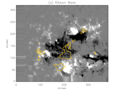
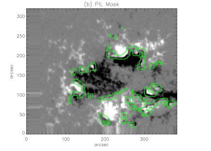
Figure 1: (a) Contours of derived ribbon mask overlain on the interpolated full-disk MDI magnetogram for event # 9. (b) Contours of derived PIL regions over the same magnetogram. The magnetograms are displayed with a saturation level of 500 Mx cm^-2, and the white areas represent positive fields whereas black areas represent negative fields.

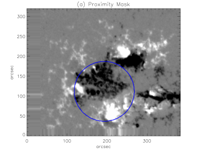
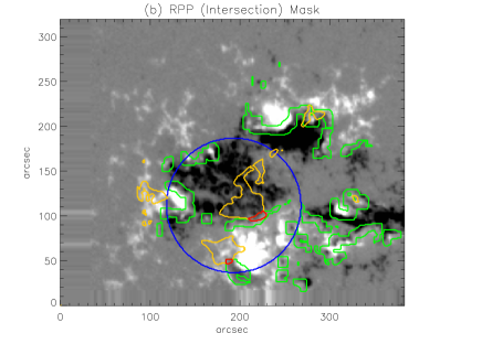
Figure 2: (a) Contours of a circular mask of radius 75 pixels centered at the mean position of ribbon pixels. (b) RPP pixels (red) lie in the intersection of ribbon mask (yellow), PIL regions (green), and the circular mask (blue). The PIL region is selected with a threshold of 100 Mx cm^-2. The potential field extrapolation was carried out above all red pixels.

Having defined the source region for this event, the extrapolation can be carried out. Using a Green’s function method, horizontal magnetic field strengths at points above the selected pixels were calculated from the line of sight field strengths of all other points in the magnetogram. This is done at heights of $\{46.5,59.2,72.3,85.8,99.9,114.5\}$ Mm. According to our assumed power-law relation between CME speeds and the transverse field strengths, the power-law index $\gamma$ is $-2.26\pm 0.2$ using Method 1 and $-2.09\pm 0.3$ using Method 2.

How robust is our estimate of this decay index? To find out, we conducted several tests, which we outline in the following paragraphs.

To start, we tried some different parameters when deriving some of the key components for extrapolation to test the robustness of our methods. First, we note that when selecting the PILs, we used a rather high threshold 100 Mx cm^-2 to exclude insignificant PILs. This substantially reduces the number of pixels identified for potential field calculation. To see if including more pixels would alter the result, we lowered the threshold to 50 Mx cm^-2. Figure 3a shows the new PIL areas selected, which encompass many more pixels than with the higher threshold (Figure 1b). Following the same extrapolation and fitting procedures, we determined the decay index from Method 1 to be -2.15, which is slightly lower than what we found with fewer pixels. This is expected since we now include some peripheral pixels with weaker fields. Still, this result is within one standard deviation of the original, indicating that original approach is robust.

Also, we note that there are bad margins present in magnetograms for some of the events, including both this example and events $\#1$, $\#3$, $\#4$, $\#5$, $\#11$, $\#12$, $\#15$ and $\#16$. In these cases, field values are replicated from the edge of the estimated chromospheric field values to the margins of the magnetogram arrays. How significantly do these artifacts affect our estimated decay indices? To investigate the effect of bad margins on our decay index estimate for this particular event, we excluded the artifacts by setting the field there to zero (Figure 3b). The resulting $\gamma$ from Method 1 based on this modified magnetogram is -2.31 which is slightly higher than originally computed but also within one standard deviation.

It is possible that the limited fields of view of our magnetograms could also affect our estimated decay indices, since fields outside of our magnetograms are ignored. But even within a magnetogram, how sensitively do our estimated decay indices depend upon magnetic flux relatively far from the flaring region? To see if our use of limited information matters, we decided to restrict our information to a circle with radius 150 pixels at the weighted event center. This specific radius was chosen because in the extrapolation for this event, the range of the heights are roughly comparable to 150 pixels and it is believed that, for the Green’s function extrapolation of a localized source distribution, the main contribution of the field at height $H$ comes from fields with a circle of radius $H$ centered at that point. A new test magnetogram was then obtained by setting the line-of-sight field outside the circle to zero. For this test, the decay index computed by Method 1 is -2.17, which is again only slightly different from our original value. This suggests that relatively distant magnetic flux should not significantly alter our estimates. These tests suggest that our original approach for estimating $\gamma$ values do not depend sensitively on our parameter choices or details of the magnetograms that we analyze.

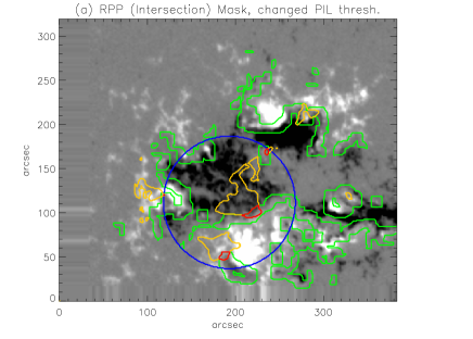
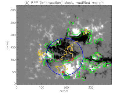
Figure 3: (a) We show ribbon pixels (yellow), the proximity threshold (blue), PILs regions (green), and RPP pixels (red), but with the PIL regions determined using a different threshold: 50 Mx cm^-2 instead of the 100 Mx cm^-2 used in Figure 2b. Comparison with that figure shows that more RPP pixels are identified, including a new, small patch separated from the other patches. (b) The same quantities, but with the original PIL threshold, and the magnetic field artifacts at the magnetogram margins set to zero. Changes in neither the PIL threshold nor magnetogram margins significantly affect $\gamma$.

4 Results

Following the approach discussed above, we carried out potential field extrapolation for all 16 events, for all masks with nonzero ribbon pixels. We then computed the decay index based on these extrapolations. The speed of each CME, $v_{\rm CME}$, was taken from the CDAW CME list. A significant correlation between CME speeds ($v_{\rm CME}$), ribbon fluxes ($\psi$), and decay indices ($\gamma$) was found. The CME speed data and ribbon flux yield a linear correlation coefficient of 0.76, with coefficient of determination 0.58; see Figure 5a. The scatter plot of $v_{\rm CME}$ versus $\gamma$ in Figure 5b also shows a clear correlation, with a linear correlation coefficient of -0.36, and coefficient of determination 0.13. A negative correlation between $\gamma$ — in which more negative values correspond to more rapidly decaying fields — and CME speeds accords with stronger overlying fields exerting stronger downward tension forces that lower the speeds of CMEs. To account for these mutual correlations, we compute the partial correlation between CME speed residuals and $\gamma$, which excludes the effect of flux $\psi$ in both variables. This yields a correlation of -0.44 with coefficient of determination 0.19; see Figure 4. The existence of a residual correlation implies that extra information about CME speeds is contained in the decay index that is not accounted for by the ribbon flux. So, while it is plausible that $\gamma$ and $\psi$ might be physically related (i.e., not physically independent variables), neither is redundant.

Figure 4: Scatter plot of CME speeds’ residual dependence on $\gamma$, after removal of the dependence of both speeds and $\gamma$ upon ribbon flux $\psi$.

Accordinly, we must characterize the joint dependence of $v_{\rm CME}$ on $\gamma$ and $\psi$. To do so, we fitted the CME speeds with a two-variable linear regression on $\psi$ and $\gamma$, with all three variables standardized (i.e., the mean of each was removed, and the result was scaled by its standard deviation). The linear regression line was calculated to be

$$v_{\rm CME}=0.73\psi-0.29\gamma~{},$$ (2)

where $v_{\rm CME}$ is the standardized speed and $\psi$ is the standardized magnetic flux. (Note that our use of standardized variables here implies that no constant term is fitted in the model.) The multiple correlation coefficient — the correlation between the predicted and actual speeds — is 0.81, with a coefficient of determination of 0.66. For linearly related variables with Gaussian deviations, a coefficient of determination equal to one would imply that the dependent variable is completely determined by the independent variables; the difference between this coefficient and one is the fraction of variance unexplained by the independent variable(s). Under these assumptions, the increase in coefficient of determination from 0.58 for $\psi$ alone to 0.66 for both $\psi$ and $\gamma$ represents a roughly 20% decrease in unexplained variance. Clearly, even with both variables, a substantial fraction of the variability in CME speeds remains unaccounted for.

To characterize the sensitivity of our results to the particular set of 16 events that comprise our sample, we estimated the variances in our results using a delete-1 jackknife procedure (Efron, 1982), i.e., by running our regression analysis on each of 16 subsets created from our event sample, each with one event deleted. We found the mean coefficient of $\psi$ in our regression to be 0.736 with standard deviation 0.034, and the mean coefficient of $\gamma$ to be -0.293 with standard deviation 0.062. Applying the delete-1 procedure to our standardized variables implies the means of each variable in the resulting 15-event subsets depart from zero, i.e., the subsets are no longer standardized. In this case, our regression procedure also generally returns a nonzero constant term. The mean and standard deviation of the fitted constant terms are 0.0036 and 0.045, respectively. Finally, we found the mean and standard deviation of the coefficient of determination to be 0.66 and 0.045, respectively.

Our use of standardized variables implies that the independent variables in Equation (2) enter with equal weight, implying their predictive power can be directly compared from their regression coefficients. Consequently, the larger coefficient for $\psi$, 0.73 versus 0.29 for $\gamma$, implies that ribbon fluxes are much stronger predictors of CME speeds than decay indices.

In Figure 6a, we plot the predicted CME speeds, based upon the regression in Equation (2), versus the actual CME speeds. The histogram of residuals between the actual CME speeds and the linear regression predictions is plotted in Figure 6b, computed in physical units. Discrepancies tend to be larger for very fast CMEs, compensated by a slight tendency for the model to overestimate speeds: there are 9 overestimates versus 7 underestimates. The outlier at the right end corresponds to event number 5. It is plausible that CME dynamics depend non-linearly on the variables we consider, instead of the linear dependence that we assume; but discriminating between the linear model and a more complex model would require a larger event sample.

Also, inspired by the work of Robbrecht, Patsourakos, and Vourlidas (2009) on stealth CMEs —CMEs observed without “low coronal signatures” — we plotted flux and gamma as a function of CME speed to see if there were some lower bounds for flux and decay index below which there is no eruption at all. The flux versus CME speeds plot in Figure 5a suggests that there is no minimum ribbon flux required for CMEs, a result expected given reports of stealth CMEs. Usually such CMEs are slow ($\approx 300$ km s^-1; Ma et al. 2010), and in order for a CME to be accelerated to a speed greater that the ambient speed of the solar wind ($\approx 450$ km s^-1), a significant amount of coronal magnetic reconnection, with consequent ribbon fluxes, appears necessary. In contrast, our fit of speeds versus $\gamma$ implies that, statistically, a minimum absolute value of $\gamma$ around 1.6 is required for CMEs. In our sample, though, several CMEs actually occur even with values of $\gamma$ less than this, highlighting that the fitted threshold is statistical.

Figure 5: (a) Ribbon fluxes as a function of CME speeds. (b) Gamma as a function of CME speeds. Event numbers are shown with each plotted symbol.

5 Discussion

We have investigated the combined roles of (i) flare ribbon flux, $\psi$, and (ii) the decay rate of overlying fields, $\gamma$, in a set of 16 eruptive events. We have confirmed previous results that higher CME speeds are associated with both larger ribbon fluxes and more rapidly decaying overlying fields. Comparing the two effects, we found that CME speeds depend more strongly on ribbon fluxes than the rate of decay of overlying fields.

Using a simple linear regression, we found that these two factors alone can explain 66% of the variation in CME speeds. Given existing routine observations of (i) photospheric magnetic fields and (ii) EUV and/or H$\alpha$ emission that can be used to identify flare ribbons, our results suggest that observers can readily make an approximate prediction of the speed of a flare-associated CME at the time of its eruption, prior to its appearance in a coronagraph. In terms of fractional errors in the predicted speeds of the relatively fast, halo CMEs in our sample, our mean $|dv|/v$ is 25%, and our mean $dv/v$ is -10%. Velocity estimates based on our results could be incorporated into existing CME propagation models (e.g., Zhao and Dryer 2014). Independent of variations in CME speeds due to acceleration occurring in interplanetary space, our errors in predicting CME speeds imply mean signed and unsigned errors in CME arrival times of 4 h and 10 h, respectively. This compares favorably with the current approach of fitting displacements of CME structure in LASCO image sequences (e.g., Mays et al. 2015), although we have only analyzed a small sample.

We note that, compared to the study by Qiu and Yurchyshyn (2005), we included some additional events. In our study, we found that the correlation of CME speeds with ribbon fluxes was weaker than the correlation they reported. We hypothesize that either the effect of outliers in their smaller sample or new events within our larger sample are responsible for the difference.

We remark that $\gamma$ values might depend significantly upon the method used to determine the potential field. Before we extrapolated fields using the Green’s function method, we first tried using PFSS models to estimate $\gamma$ above active regions in a sample of 47 CMEs. Following essentially the same PIL identification method discussed above (but without ribbon observations to identify which PIL regions were involved in these flares), we calculated the decay index $\gamma$ above PILs in these regions. In Table 2, we compare our results from the Green’s function method used described above with $\gamma$’s estimated from PFSS models. We find that Green’s function $\gamma$’s are systematically more negative than PFSS $\gamma$s, implying more rapid decrease of horizontal field strength with height.

Given the similar approaches used, why do the inferred values for $\gamma$ differ systematically? First, it should be noted that these two sets of extrapolations were done above different sets pixels, which might by itself explain the differing $\gamma$ values. But the difference might also be due to the lower spatial resolution of typical PFSS models (ours used spherical harmonics up to $\ell=$ 192), which yield smaller field strengths at low coronal heights. While our Green’s function method treats each pixel in the magnetogram as a single, delta-function source, PFSS models typically integrate over pixels to compute spherical harmonic coefficients. In this way, small bipoles (positive and negative flux close to each other) can get averaged out in low-resolution PFSS models, thus not contributing to the extrapolated field. With their better resolution, however, Green’s function methods can incorporate fields from small-scale bipoles into the extrapolations. Since the dipole moments from these small-scale fields are quite strong just above the photosphere but decay relatively rapidly with height, the field strengths computed using Green’s functions probably systematically decrease faster with height than PFSS fields, resulting in a more negative $\gamma$. A more detailed study comparing methods of estimating decay indices would be worthwhile.

Why do CME speeds depend more strongly on ribbon fluxes than decay indices? One possibility is that this is an artifact of our approach: since we only studied events with successful CME onset, we did not take into account the fact that there might be failed eruptions due to downward tension caused by overlying fields (e.g., Wang and Zhang 2007; Liu 2008). In this sense, part of the effect of the decay rate of the overlying field on a CME eruption is obscured compared to the effect of ribbon fluxes: $\gamma$ might need to be negative enough for an eruption to be permitted at all, i.e., a high enough decay rate might be a necessary condition for an eruption in the first place. (Given that Xu et al. (2012) report eruptions for a very wide range of $\gamma$ values, however, it is not clear if any meaningful threshold in $\gamma$ exists.) Another possiblity is that potential field models are too inaccurate: perhaps discrepancies between the potential and actual magnetic fields above eruption sites are significant enough that our estimates for decay indices are wrong. Or perhaps decay indices themselves are irrelevant: maybe lateral motions in the early stages of eruptions enable CMEs to erupt “sideways” rather than pushing through overlying fields as we assume.

Ultimately, it is clear that factors other than just the two that we consider also govern CME speeds. Likely possibilities include the internal magnetic structure of the pre-flare magnetic system that later erupts (e.g., the amount of flux within this system, and / or the degree of its initial magnetic twist, perhaps quantified by magnetic helicity) and interplanetary magnetic field and density structures (including the effects of previous CMEs). We also remark that the CME speeds that we cite are plane-of-sky speeds; CMEs’ true speeds might be faster, which is an additional source of discrepancy between our simplistic model and the observations.

Figure 6: (a) A scatter plot of actual CME speeds vs. predicted values. (b) Histogram of deviations of actual CME speeds from the linear regression predictions, in original units.

Table 1: Under CME Label, data sources are identified by H(H$\alpha$) and T(TRACE). We note that compared to Qiu and Yurchyshyn (2005) and Qiu et al. (2007), we add event $\#1$ and $\#2$. The information about date, time and speed of these events are from CDAW CME list, and the information about location and AR number are from UH IfA active region label maps. TRACE’s $0.^{\prime\prime}5$ pixels were summed 2 x 2. The * in the Decay indices (Method 2) of events $\#6$ and $\#8$ denotes that in the calculation of $\gamma$ for the two events, there is only one pixel in the RPP regions, thus precluding estimating standard deviations.

CME	Date	Time	Location	$v_{\rm CME}$	AR	Gamma	Gamma	Flux	Pixel
Label		[hh:mm:ss]		[km s-1]	#	(Method 1)	(Method 2)	[1021Mx]	size (′′)
1(H)	2000 Jan 18	16:03:02	S18E14	739	8831	$-1.32\pm 0.1$	$-1.28\pm 0.1$	$0.55\pm 1.1$	1.16
2(T)	2000 Jul 25	01:39:01	N06W01	528	9097	$-1.80\pm 0.4$	$-1.79\pm 0.3$	$0.9\pm 0.2$	1
3(H)	2000 Aug 09	14:23:01	N11W01	702	9114	$-1.98\pm 0.1$	$-2.07\pm 0.1$	$1.8\pm 1.5$	1.05
4(H)	2000 Nov 24	20:48:02	N21E06	1000	9236	$-2.66\pm 0.2$	$-3.12\pm 0.5$	$1.7\pm 0.3$	1.12
5(T)	2001 Apr 10	04:48:02	S22W07	2411	9415	$-2.55\pm 0.1$	$-2.19\pm 0.1$	$4.9\pm 0.5$	1
6(T)	2001 Apr 26	09:36:03	N16W15	1006	9433	$-1.47\pm 0.2$	$-1.47*$	$1\pm 1.4$	1
7(H)	2001 Sep 28	07:59:02	N13E26	846	9636	$-1.69\pm 0.1$	$-1.75\pm 0.1$	$4.4\pm 0.6$	1.07
8(H)	2002 Mar 20	16:00:01	S19W06	603	9871	$-1.28\pm 0.1$	$-1.30*$	$1.7\pm 0.3$	1.07
9(H)	2002 Jul 26	19:11:00	S16E34	818	10039	$-2.26\pm 0.2$	$-2.09\pm 0.3$	$2.6\pm 1.3$	1
10(T)	2003 Oct 28	09:35:03	S16E18	2459	10486	$-1.29\pm 1.3$	$-0.79\pm 1.0$	$22\pm 3.2$	1
11(T)	2003 Oct 29	19:11:03	S17E04	2029	10486	$-3.37\pm 0.3$	$-3.32\pm 0.4$	$13\pm 1.2$	1
12(T)	2003 Nov 18	06:23:03	N03E35	1660	10501	$-1.90\pm 0.2$	$-2.02\pm 0.2$	$3.2\pm 0.9$	1
13(T)	2004 Nov 07	14:23:03	N09W08	1759	10696	$-2.30\pm 0.1$	$-2.31\pm 0.1$	$5.6\pm 0.7$	1
14(H)	2005 May 13	16:03:02	N12E19	1642	10759	$-1.99\pm 0.3$	$-1.95\pm 0.1$	$7.9\pm 0.5$	1.07
15(H)	1998 Apr 29	15:59:04	S17E30	1374	8210	$-2.26\pm 0.1$	$-2.20\pm 0.1$	$4.1\pm 0.5$	1.04
16(H)	1998 Nov 05	15:36:04	N18W07	1118	8375	$-2.05\pm 0.5$	$-2.09\pm 0.2$	$3.7\pm 0.6$	1.04

Table 2: In this table, we compare $\gamma$’s computed using Method 1 with our Green’s function method with $\gamma$’s from PFSS models for an overlapping set of seven events. Apparently the magnitudes of $\gamma$’s computed from PFSS models are either about the same or smaller that $\gamma$’s computed with Method 1.

Event	$\gamma$,	$\gamma$,
Number	Green’s function	PFSS
1	$-1.32\pm 0.09$	$-1.03\pm 0.152$
4	$-2.66\pm 0.156$	$-1.11\pm 0.108$
5	$-2.26\pm 0.144$	$-2.17\pm 0.281$
6	$-1.47\pm 0.187$	$-1.51\pm 1.037$
10	$-1.29\pm 1.29$	$-1.30\pm 0.101$
11	$-3.37\pm 0.278$	$-1.15\pm 0.120$
14	$-1.99\pm 0.259$	$-1.03\pm 0.046$

References

- Brueckner et al. (1995) Brueckner, G.E., Howard, R.A., Koomen, M.J., Korendyke, C.M., Michels, D.J., Moses, J.D., Socker, D.G., Dere, K.P., Lamy, P.L., Llebaria, A., Bout, M.V., Schwenn, R., Simnett, G.M., Bedford, D.K., Eyles, C.J.: 1995, The Large Angle Spectroscopic Coronagraph (LASCO). Solar Phys. 162, 357. DOI.
- Démoulin and Aulanier (2010) Démoulin, P., Aulanier, G.: 2010, Criteria for flux rope eruption: Non-equilibrium versus torus instability. Astrophys. J. 718, 1388. DOI. ADS.
- Efron (1982) Efron, B.: 1982, The Jackknife, the Bootstrap and Other Resampling Plans. CBMS-NSF Regional Conference Series in Applied Mathematics, 38, Society for Industrial and Applied Mathematics (SIAM), Philadelphia. ADS.
- Forbes and Priest (1984) Forbes, T.G., Priest, E.R.: 1984, Reconnection in solar flares. In: Butler, D.M., Papadopoulos, K. (eds.) Solar Terrestrial Physics: Present and Future, NASA Reference Publ. 1120., 1.
- Gopalswamy et al. (2010) Gopalswamy, N., Akiyama, S., Yashiro, S., Mäkelä, P.: 2010, Coronal mass ejections from sunspot and non-sunspot regions. In: Hasan, S.S., Rutten, R.J. (eds.) Magnetic Coupling between the Interior and Atmosphere of the Sun, Springer, Berlin, Heidelberg, 289. DOI. ADS.
- Gosling (1993) Gosling, J.T.: 1993, The solar flare myth. J. Geophys. Res. 98(A11), 18,937.
- Handy et al. (1999) Handy, B.N., Acton, L.W., Kankelborg, C.C., Wolfson, C.J., Akin, D.J., Bruner, M.E., et al.: 1999, The Transition Region and Coronal Explorer. Solar Phys. 187, 229. DOI. ADS.
- Kliem and Török (2006) Kliem, B., Török, T.: 2006, Torus instability. Phys. Rev. Lett. 96(25), 255002. DOI.
- Liu (2008) Liu, Y.: 2008, Magnetic field overlying solar eruption regions and kink and torus instabilities. Astrophys. J. Lett. 679, L151. DOI.
- Ma et al. (2010) Ma, S., Attrill, G.D.R., Golub, L., Lin, J.: 2010, Statistical study of coronal mass ejections with and without distinct low coronal signatures. Astrophys. J. 722, 289. DOI. ADS.
- Mays et al. (2015) Mays, M.L., Taktakishvili, A., Pulkkinen, A., MacNeice, P.J., Rastätter, L., Odstrcil, D., et al.: 2015, Ensemble Modeling of CMEs Using the WSA-ENLIL+Cone Model. Solar Phys. 290, 1775. DOI. ADS.
- Poletto and Kopp (1986) Poletto, G., Kopp, R.A.: 1986, Macroscopic electric fields during two-ribbon flares. In: Neidig, D.F. (ed.) The Lower Atmosphere of Solar Flares; Proceedings of the Solar Maximum Mission Symposium, National Solar Observatory, Sunspot, NM, 453. ADS.
- Qiu and Yurchyshyn (2005) Qiu, J., Yurchyshyn, V.B.: 2005, Magnetic reconnection flux and coronal mass ejection velocity. Astrophys. J. Lett. 634, L121. DOI. ADS.
- Qiu et al. (2004) Qiu, J., Wang, H., Cheng, C.Z., Gary, D.E.: 2004, Magnetic reconnection and mass acceleration in flare-coronal mass ejection events. Astrophys. J. 604, 900. DOI.
- Qiu et al. (2007) Qiu, J., Hu, Q., Howard, T.A., Yurchyshyn, V.B.: 2007, On the magnetic flux budget in low-corona magnetic reconnection and interplanetary coronal mass ejections. Astrophys. J. 659, 758. DOI. ADS.
- Richardson and Cane (2011) Richardson, I.G., Cane, H.V.: 2011, Geoeffectiveness (Dst and Kp) of interplanetary coronal mass ejections during 1995-2009 and implications for storm forecasting. Space Weather 9, 7005. DOI.
- Robbrecht, Patsourakos, and Vourlidas (2009) Robbrecht, E., Patsourakos, S., Vourlidas, A.: 2009, No trace left behind: STEREO observation of a coronal mass ejection without low coronal signatures. Astrophys. J. 701, 283. DOI. ADS.
- Sakurai (1982) Sakurai, T.: 1982, Green’s function methods for potential magnetic fields. Solar Phys. 76, 301.
- Scherrer et al. (1995) Scherrer, P.H., Bogart, R.S., Bush, R.I., Hoeksema, J.T., Kosovichev, A.G., Schou, J., et al.: 1995, The Solar Oscillations Investigation - Michelson Doppler Imager. Sol. Phys. 162, 129 .
- Sterling and Moore (2001) Sterling, A.C., Moore, R.L.: 2001, Internal and external reconnection in a series of homologous solar flares. J. Geophys. Res. 106, 25227. DOI. ADS.