Spin-charge separated quasiparticles in one dimensional quantum fluids

Abstract

We revisit the problem of dynamical response in spin-charge separated one dimensional quantum fluids. In the framework of Luttinger liquid theory, the dynamical response is formulated in terms of noninteracting bosonic collective excitations carrying either charge or spin. We argue that, as a result of spectral nonlinearity, long-lived excitations are best understood in terms of generally strongly interacting fermionic holons and spinons. This has far reaching ramifications for the construction of mobile impurity models used to determine threshold singularities in response functions. We formulate and solve the appropriate mobile impurity model describing the spinon threshold in the single-particle Green’s function. Our formulation further raises the question whether it is possible to realize a model of noninteracting fermionic holons and spinons in microscopic lattice models of interacting spinful fermions. We investigate this issue in some detail by means of density matrix renormalization group (DMRG) computations.

I Introduction

Understanding the essential features of a quantum many-body system usually entails finding a simple explanation of its low-energy spectrum in terms of weakly interacting, long-lived quasiparticles. For example, in Landau’s Fermi liquid theory the quasiparticles are fermions carrying the same quantum numbers as an electron, namely charge $e$ and spin 1/2. However, it is well established that the long lived excitations in strongly correlated systems may carry only a fraction of the quantum numbers of the elementary constituents. In fact, fractionalization is often invoked as a route towards exotic phases of matter such as spin liquids or high-temperature superconductors xu .

Perhaps the most prominent example of fractionalization is spin-charge separation in one dimensional (1D) quantum fluids known as Luttinger liquids deshpande . The hallmark of these theories is a low energy spectrum described by two decoupled free bosonic fields associated with collective spin and charge degrees of freedom, respectively. On the experimental side, the most direct evidence for spin-charge separation involves the observation of multiple peaks associated with spin and charge collective modes in dynamical response functions at fairly high energies auslaender ; kim ; jompol ; schlappa , beyond the regime where Luttinger liquid theory is applicable. Spin-charge separation is known to persist at high energies for integrable theories such as the 1D Hubbard hubbardbook ; EK94a ; EK94b ; Andrei ; Deguchi ; penc1 ; favand ; penc ; benthien ; adrian and $1/r^{2}$ $t$-$J$arikawa01 ; arikawa04 models. In these cases any eigenstate with a finite energy in the thermodynamic limit can be classified in terms of elementary excitations called holons (which carry charge $e$ and spin 0) and spinons (which carry charge 0 and spin $1/2$), along with their bound states. A convenient way for describing such excitations as well as their scattering is to define corresponding creation and annihilation operators $Z^{\dagger}_{a}(\theta)$ and $Z_{a}(\theta)$, where $a$ labels the different types of elementary excitations and $\theta$ is a variable that parameterizes the momentum $p_{a}(\theta)$ (the form of this function depends on the particular model under consideration). As a consequence of integrability, creation and annihilation operators fulfil the Faddeev-Zamolodchikov algebra Zam ; Fadd

$$Z_{a}(\theta_{1})Z_{b}(\theta_{2}) = S_{ab}^{cd}(\theta_{1},\theta_{2})Z_{d}(\theta_{2})Z_{c}(\theta_{1}),$$

$$Z_{a}(\theta_{1})Z^{\dagger}_{b}(\theta_{2}) = 2\pi\delta(\theta_{1}-\theta_{2})\delta_{a,b}$$ (1)

$$+S_{bc}^{da}(\theta_{2},\theta_{1})Z^{\dagger}_{d}(\theta_{2})Z_{c}(\theta_{1}).$$

Here $S_{ab}^{cd}(\theta_{1},\theta_{2})$ is the purely elastic two-particle S-matrix. The corresponding elementary excitations are infinitely long lived, but generally strongly interacting, as can be seen from their scattering matrices EK94a ; EK94b ; Andrei . Moreover, their quantum numbers, e.g. charge 0 and spin 1/2 for spinons in the Hubbard model, differ from those of the collective bosonic spin modes in the Luttinger liquid description. It is natural to assume that breaking integrability slightly will not generically lead to a qualitative change in the nature of elementary holon and spinon excitations, but merely render the lifetimes finite.

How to reconcile this picture emerging from the exact solution with Luttinger liquid theory? In the latter, the nature of elementary excitations is obscured by the fact that, due to the linear dispersion approximation, the spectrum is highly degenerate and allows for many interpretations, which ultimately all give the same results for physical observables. Examples are chiral Luttinger liquid descriptions of quantum Hall edges kareljan and the low-energy excitations of the Hubbard model. The latter can be understood both in terms of interacting, fermionic holons and spinons JNW ; hubbardbook ; woynarovich ; frahmkorepin , and in terms of noninteracting bosons associated with collective spin and charge degrees of freedom Affleck ; gogolin ; giamarchi .

Going beyond the linear dispersion approximation is expected to remove ambiguities in the quasiparticle description of the spectrum: there will be a particular choice that maximizes the lifetimes of elementary excitations. In integrable models such as the Hubbard chain these lifetimes are infinite.

Over the last decade it has been established in a series of works that going beyond the linear dispersion approximation is essential for correctly describing the dynamics of one dimensional models with gapless excitations work1 ; rozhkov ; Roz06 ; work2 ; carmelo1 ; carmelo2 ; carmelo3 ; BAW1 ; work3 ; work4 ; work5 ; IG08 ; work6 ; BAW2 ; ABW ; work7 ; work8 ; PWA09 ; pereira12 ; Roz14 ; austen ; PS ; Pereira ; SIG1 ; SIG2 ; FHLE ; SIG3 ; ts ; Seabra . This has resulted in the so-called “nonlinear Luttinger liquid” (nLL) approach to gapless 1D quantum liquids; see Refs. SIG3, ; pereira12, for recent reviews. The basic reason for the failure of linear Luttinger liquid theory is that at finite energies the running coupling constants of irrelevant perturbations such as band curvature terms are in fact different from zero. Taking them into account in perturbation theory leads to infrared singularities. These need to be resummed to all orders in the coupling constants, which gives rise to new, momentum-dependent exponents in response functions.

A key ingredient of the nLL method is the identification of quasiparticles describing excited states both at high and at low energies. This is straightforward for spinless fermions, because the quasiparticles are adiabatically connected to free fermions PWA09 . The spinful case is considerably more involved due to the onset of spin-charge separation for arbitrarily weak interactions and the concomitant qualitative change in the nature of the elementary excitations compared to the noninteracting limit. It was realized in Refs. PS, ; SIG1, ; SIG2, ; Pereira, that in many important cases exact results can be obtained by using a phenomenological model of weakly interacting fermionic holons and spinons, whose dispersions delineate the edges of the support of the dynamical response function under consideration. By construction these excitations are different from the true elementary excitations in the Hubbard model. In particular, they carry different spin and charge quantum numbers. It is then an obvious but crucial question how to reconcile this approach with the exact solution of integrable models like the Hubbard chain.

In this work we develop a new approach to deriving mobile impurity models for studying dynamical correlations in gapless models of spinful fermions. We first carry out a direct construction of the “physical” holon and spinon fields in the limit of weak electron-electron interactions. This results in a representation of spinful nonlinear Luttinger liquids in terms of strongly interacting holons and spinons, which is in direct accord with known results obtained in integrable cases. Recalling that the spinless fermion case was best understood by considering weak interactions, we address the construction of a microscopic model of interacting electrons giving rise to a theory of noninteracting fermionic holons and spinons at low energies, but in presence of spectral nonlinearities. We then derive mobile impurity models to analyze dynamical response functions in our formulation. We demonstrate explicitly how to recover results obtained previously by means of the approach of Refs. SIG1, ; SIG2, . Finally, we address the question how to realize a lattice model of interacting electrons that gives rise to noninteracting holons and spinons at low energies.

II Spinless Fermions

Before we approach the problem of defining quasiparticles for spin-$1/2$ fermions, it is instructive to review the case of spinless fermions. For concreteness, consider the simplest lattice model of interacting spinless fermions:

$$H=-t\sum_{j=1}^{L}(c^{\dagger}_{j}c^{\phantom{\dagger}}_{j+1}+\textrm{h.c.})+V\sum_{j}n_{j}n_{j+1}.$$ (2)

Here $c_{j}$ is the annihilation operator for a fermion at site $j$, $n_{j}=c^{\dagger}_{j}c^{\phantom{\dagger}}_{j}$ is the number operator, $t$ is the hopping parameter, and $V$ is the nearest-neighbor interaction strength. This model has a U(1) symmetry, $c_{j}\to e^{i\alpha}c_{j}$, $\alpha\in\mathbb{R}$, associated with conservation of the total number of fermions $N$. Moreover, the model is integrable and the exact spectrum for arbitrary values of $V$ can be calculated from the Bethe ansatz solution korepinbook ; Faddeev84 . There is a gapless phase extending between $-2<V\leq 2$. At $V=2$ the model is equivalent to the SU(2)-symmetric Heisenberg spin chain korepinbook .

A useful starting point for analytical approximations is the noninteracting model with $V=0$. In this case, the elementary excitations are free fermions with dispersion relation $\epsilon_{0}(k)=-2t\cos k-\mu$ measured from the Fermi energy $\mu$. Low-energy excitations are particles and holes with momentum close to the Fermi points, $k\approx\pm k_{F}$. The Fermi momentum is related to the average density by $k_{F}=\pi N/(La_{0})$, where $a_{0}$ is the lattice spacing.

At weak coupling, $V/t\ll 1$, standard bosonization can be used to derive an effective low-energy theory for model (2), see e.g. Refs. Affleck, ; gogolin, ; review, . One starts by taking the continuum limit and projecting the fermionic field onto states with momentum near the Fermi points. This leads to the right- and left-moving components in the mode expansion

$$c_{j}\to\sqrt{a_{0}}[e^{ik_{F}x}R(x)+e^{-ik_{F}x}L(x)].$$ (3)

The effective Hamiltonian in terms of $R$ and $L$ fermions reads

$$\mathcal{H} = \int dx[-v^{\prime}R^{\dagger}i\partial_{x}R+v^{\prime}L^{\dagger}i\partial_{x}L$$ (4)

$$+gR^{\dagger}RL^{\dagger}L+\mathcal{H}_{\textrm{irr}}(x)],$$

where all operators are normal ordered with respect to the noninteracting Dirac sea. To first order in $V$, we have the parameters $v^{\prime}\approx 2ta_{0}\sin k_{F}\left(1+\frac{V}{\pi t}\sin k_{F}\right)$ and ${g\approx 4Va_{0}\sin^{2}k_{F}}$. The coupling constant $g$ is the only marginal interaction. The term $\mathcal{H}_{\textrm{irr}}(x)$ contains nonlinear dispersion terms and other interactions which are irrelevant in the renormalization group (RG) sense. In the standard Luttinger liquid approach this term is dropped, which corresponds to linearizing the dispersion around the Fermi points $\pm k_{F}$.

The bosonization formula for chiral spinless fermions reads

$$R(x) = \frac{\eta}{\sqrt{2\pi}}\,e^{-\frac{i}{\sqrt{2}}\varphi(x)},$$ (5)

$$L(x) = \frac{\bar{\eta}}{\sqrt{2\pi}}\,e^{\frac{i}{\sqrt{2}}\bar{\varphi}(x)},$$ (6)

where $\eta,\bar{\eta}$ are Majorana fermions and $\varphi(x),\bar{\varphi}(x)$ are chiral bosons that obey the commutation relations

$$[\varphi(x),\bar{\varphi}(y)] = 0,$$ (7)

$${[\varphi(x),\varphi(y)]} = 2\pi i\text{sgn}(x-y)=-[\bar{\varphi}(x),\bar{\varphi}(y)].$$ (8)

Throughout this paper we use “CFT normalizations” for bosonic vertex operators

$$\langle e^{i\alpha\varphi(x)}e^{-i\alpha\varphi(y)}\rangle=\frac{1}{(x-y)^{2\alpha^{2}}}.$$ (9)

A consequence of employing these conventions is that vertex operators are dimensionful

$${\rm dim}\left(e^{i\alpha\varphi(x)}\right)={\rm length}^{-\alpha^{2}}.$$ (10)

We also define the canonical bosonic field $\Phi(x)$ and its dual $\Theta(x)$ by

$$\Phi(x) = \varphi(x)+\bar{\varphi}(x),$$ (11)

$$\Theta(x) = \varphi(x)-\bar{\varphi}(x),$$ (12)

which obey

$$[\Phi(x),\Theta(x^{\prime})]=4\pi i\text{sgn}(x-x^{\prime}).$$ (13)

Bosonization of Eq. (4) then leads to the Hamiltonian

$$\mathcal{H}=\int dx[\mathcal{H}_{\textrm{LL}}(x)+\mathcal{H}_{\textrm{irr}}(x)].$$ (14)

The first term,

$$\mathcal{H}_{\textrm{LL}}(x)=\frac{v}{16\pi}\left[K(\partial_{x}\Theta)^{2}+\frac{1}{K}(\partial_{x}\Phi)^{2}\right],$$ (15)

is the Luttinger model. The velocity $v$ and the Luttinger parameter $K$ are given to first order in $V$ by $v\approx v^{\prime}$ and $K\approx 1-\frac{V}{\pi t}\sin k_{F}$. The bosonic fields describe the collective low-energy density mode of the quantum fluid. The uniform part of the density operator is related to $\Phi(x)$ by the bosonization relation

$$Q(x)=R^{\dagger}(x)R(x)+L^{\dagger}(x)L(x)\sim-\frac{1}{\pi\sqrt{8}}\partial_{x}\Phi(x).$$ (16)

The total charge operator is given by the integral

$$q=\int_{-\infty}^{+\infty}dx\,Q(x).$$ (17)

Thus, an elementary excitation with charge $q=1$ corresponds to a kink of amplitude $\pi\sqrt{8}$ in the bosonic field $\Phi(x)$. As is well known, the model in Eq. (15) correctly captures the long-distance asymptotic decay of correlation functions for any 1D system in the Luttinger liquid universality class Affleck ; gogolin ; giamarchi .

The limitations of Luttinger liquid theory appear when one considers dynamical response functions at small but finite frequency and momentum. At finite energy scales it becomes necessary to take the irrelevant perturbations ${\cal H}_{\rm irr}$ to the Luttinger model into account. At weak coupling and in the absence of particle-hole symmetry (i.e. away from half-filling in the lattice model), the leading corrections in (4) are the dimension-three operators

$$\mathcal{H}_{\textrm{irr}} = -\frac{1}{2\tilde{m}}(R^{\dagger}\partial_{x}^{2}R+L^{\dagger}\partial_{x}^{2}L)$$ (18)

$$+g_{3}(R^{\dagger}RL^{\dagger}i\partial_{x}L-L^{\dagger}LR^{\dagger}i\partial_{x}R+\textrm{h.c.}).$$

Here we have introduced $\tilde{m}^{-1}\approx m^{-1}+\frac{Va_{0}^{2}}{\pi}\sin 2k_{F}$, with $m^{-1}=2ta_{0}^{2}\cos k_{F}$ the inverse free fermion mass, and $g_{3}\approx Va_{0}^{2}\sin 2k_{F}$. Bosonizing these irrelevant terms we obtain cubic boson-boson interactions

$$\mathcal{H}_{\textrm{irr}} = \lambda_{3}^{+}\partial_{x}\Phi[(\partial_{x}\Phi)^{2}+(\partial_{x}\Theta)^{2}]$$ (19)

$$+\lambda_{3}^{-}\partial_{x}\Phi[(\partial_{x}\Phi)^{2}-(\partial_{x}\Theta)^{2}],$$

with $\lambda_{3}^{+}\approx-\frac{1}{48\sqrt{2}\pi}\left[\frac{1}{m}+\frac{g_{3}}{\pi}\right]$ and $\lambda_{3}^{-}\approx\frac{1}{96\sqrt{2}\pi}\left[\frac{1}{m}-\frac{2g_{3}}{\pi}\right]$. While the bosonic representation allows one to take the marginal interaction $g$ into account exactly, perturbation theory in the nonlinear boson interactions (19) suffers from infrared divergences work2 ; pereira12 . The latter are associated with the huge degeneracy of states in the linear dispersion approximation: all states with an arbitrary number of bosons moving in the same direction carrying the same total momentum are degenerate work2 ; pereira12 .

A way to circumvent these difficulties in analyzing the nonlinear bosonic theory is suggested by reverting to the fermionic representation (18). At the free fermion point, the irrelevant interaction vanishes, $g_{3}=0$, and one is left with the quadratic dispersion term with effective mass $m$. Taking the nonlinear dispersion into account in the free fermion model removes the degeneracy of particle-hole pairs that carry the same total momentum. One can then approach the problem from free fermions with nonlinear dispersion and include interactions perturbatively work1 . This approach reveals that the most pronounced effect of the interactions is to give rise to power-law singularities at the edges of the excitation spectrum. While a complete analytical solution of model (4) taking into account both band curvature and interaction is highly nontrivial, the edge singularities can be described by an effective impurity model in analogy with the x-ray edge problem work1 ; Schotte .

Consider, for instance, the single-fermion spectral function

$$A(\omega,k)=-\frac{1}{\pi}\text{Im }G_{\text{ret}}(\omega,k),$$ (20)

where

$$G_{\text{ret}}(\omega,k) = -i\int_{0}^{\infty}dt\,e^{i\omega t}\sum_{l}\,e^{-ikla_{0}}$$ (21)

$$\times\langle\psi_{0}|\{c^{\phantom{\dagger}}_{j+l}(t),c^{\dagger}_{j}\}|\psi_{0}\rangle$$

is the retarded Green’s function, with $|\psi_{0}\rangle$ the exact ground state. We can separate the negative- and positive-frequency parts of the spectral function:

$$A(\omega,k)=A_{<}(\omega,k)+A_{>}(\omega,k).$$ (22)

The Lehmann representation reads:

$$A_{<}(\omega,k) = 2\pi\sum_{n}|\langle\psi_{n}|c^{\phantom{\dagger}}_{k}|\psi_{0}\rangle|^{2}\delta(\omega+E_{n}-E_{0}),$$ (23)

$$A_{>}(\omega,k) = 2\pi\sum_{n}|\langle\psi_{n}|c^{\dagger}_{k}|\psi_{0}\rangle|^{2}\delta(\omega-E_{n}+E_{0}),$$ (24)

where $c_{k}$ annihilates a fermion with momentum $k$ and $|\psi_{n}\rangle$ denotes an exact eigenstate of the Hamiltonian with energy $E_{n}$. Let us focus on the negative-frequency part for $k<k_{F}$. For free fermions, we have $A^{(0)}_{<}(\omega,k)=\delta(\omega-\epsilon_{0}(k))$, where $\epsilon_{0}(k)<0$ is the energy of the particle annihilated below the Fermi surface. When weak interactions are turned on, the renormalized fermion dispersion $\epsilon(k)$ becomes a threshold of the support of $A_{<}(\omega,k)$, such that a power-law singularity develops for $\omega<\epsilon(k)$. To describe the edge singularity for fixed $k<k_{F}$, we go back to the mode expansion in Eq. (3) and generalize it to include three patches of momentum:

$$c_{j}\to\sqrt{a_{0}}[e^{ik_{F}x}r(x)+e^{-ik_{F}x}l(x)+e^{ikx}\chi^{\dagger}(x)],$$ (25)

Here the “impurity field” $\chi^{\dagger}(x)$ creates a hole in a state with momentum close to $k$, within a subband of width $\Lambda\ll k_{F}-k$. The low-energy Fermi fields $r(x)$ and $l(x)$ are also defined with a cutoff of order $\Lambda$. In the case $q=k_{F}-k\ll k_{F}$, the field $l(x)$ can be regarded as the projection of $L(x)$ into a narrower subband, while $R(x)$ is split into two separate subbands corresponding to the low-energy mode $r(x)$ and the “high-energy” mode $\chi(x)$. Restricting the energy window to the vicinity of the threshold with a single impurity, we now have to calculate the propagator of $\chi(x)$:

$$G_{\text{ret},<}(\omega,k) \approx -i\int_{0}^{\infty}dt\,e^{i\omega t}\int_{-\infty}^{\infty}dx$$ (26)

$$\times\langle\psi_{0}|\chi(0,0)\chi^{\dagger}(t,x)|\psi_{0}\rangle.$$

At weak coupling, i.e. as long as the four-fermion interaction strength $V$ is small, we can substitute Eq. (25) into Eq. (2) and bosonize the low-energy fields to derive an effective Hamiltonian for the single hole coupled to low-energy collective modes. The result is the mobile impurity model work5

$$\mathcal{H}_{\rm imp} = \int dx\Big{\{}\frac{v}{16\pi}\Big{[}K(\partial_{x}\Theta)^{2}+\frac{1}{K}(\partial_{x}\Phi)^{2}\Big{]}$$ (27)

$$+\chi^{\dagger}(\varepsilon-iu\partial_{x})\chi$$

$$+\chi^{\dagger}\chi[f(q)\partial_{x}\varphi+\bar{f}(q)\partial_{x}\bar{\varphi}]\Big{\}},$$

where $\varepsilon\equiv-\epsilon(k)>0$ is the energy of the “deep hole” excitation, $u=\frac{d\epsilon}{dk}$ is the velocity obtained by linearizing the dispersion around the centre of the impurity subband, and $f(q)$ and $\bar{f}(q)$ are momentum-dependent impurity-boson couplings of order $V$. The calculation of the Green’s function in Eq. (21) is made possible by performing a unitary transformation that decouples the impurity from the low-energy modes:

$$U=e^{-i\int_{-\infty}^{\infty}dx\,[\gamma\varphi(x)+\bar{\gamma}\bar{\varphi}(x)]\chi^{\dagger}(x)\chi(x)}.$$ (28)

The bosonic fields transform as

$$\varphi^{\circ}(x) = U\varphi(x)U^{\dagger}=\varphi(x)-2\pi\gamma C(x),$$

$$\varphi^{\circ}(x) = U\bar{\varphi}(x)U^{\dagger}=\varphi(x)+2\pi\bar{\gamma}C(x),$$ (29)

where

$$C(x)=\int_{-\infty}^{\infty}dy\,\text{sgn}(x-y)\chi^{\dagger}(y)\chi(y).$$ (30)

The transformed impurity field is

$$d(x) = U\chi(x)U^{\dagger}$$ (31)

$$= \chi(x)e^{i[\gamma\varphi(x)+\bar{\gamma}\bar{\varphi}(x)]}e^{-i\pi(\gamma^{2}-\bar{\gamma}^{2})C(x)}.$$

Note that the impurity density is invariant under the unitary transformation, i.e. $\chi^{\dagger}(x)\chi(x)=d^{\dagger}(x)d(x)$.

We choose the parameters $\gamma,\bar{\gamma}$ as the solution of

$$\left(\begin{array}[]{c}f\\ \bar{f}\end{array}\right)=\left(\begin{array}[]{cc}v_{+}-u&v_{-}\\ -v_{-}&-v_{+}-u\end{array}\right)\left(\begin{array}[]{c}\gamma\\ \bar{\gamma}\end{array}\right),$$ (38)

where

$$v_{\pm}=\frac{v}{2}\left(K\pm\frac{1}{K}\right).$$ (39)

With this choice, the Hamiltonian becomes noninteracting:

$$H_{\rm imp} = \int dx\Big{\{}\frac{v}{16\pi}\Big{[}K(\partial_{x}\Theta^{\circ})^{2}+\frac{1}{K}(\partial_{x}\Phi^{\circ})^{2}\Big{]}$$ (40)

$$+d^{\dagger}(\varepsilon-iu\partial_{x})d+\dots\Big{\}},$$

where $\dots$ stands for irrelevant operators which are neglected in the impurity model (since they only introduce subleading corrections to edge singularities). On the other hand, the expression in Eq. (26) now becomes

$$G_{\text{ret,<}}(\omega,k) \approx -i\int_{0}^{+\infty}dt\,e^{i\omega t}\int_{-\infty}^{\infty}dx\langle d^{\phantom{\dagger}}(0,0)d^{\dagger}(t,x)\rangle_{0}$$ (41)

$$\times\langle F(0,0)F^{\dagger}(t,x)\rangle_{0},$$

where $\langle\,\rangle_{0}$ denotes the expectation value in the noninteracting ground state $|\tilde{\psi}_{0}\rangle=U|\psi_{0}\rangle$ and $F(x)$ is the string operator

$$F(x)=e^{i[\gamma\varphi^{\circ}(x)+\bar{\gamma}\bar{\varphi}^{\circ}(x)]}.$$ (42)

The correlation function in Eq. (41) can then be calculated by standard methods SIG3 . The important point is that the scaling dimension of the operator $F(x)$ changes continuously as a function of $\gamma,\bar{\gamma}$. As a result, the effective impurity model predicts a power-law singularity in the spectral function,

$$A_{<}(\omega,k)\sim\theta(\epsilon(k)-\omega)|\epsilon(k)-\omega|^{-1+2(\gamma^{2}+\bar{\gamma}^{2})}.$$ (43)

Importantly, the impurity mode $\chi(x)$ in Eq. (27) carries charge $q=1$ because it is defined from the original fermion $c_{j}$ at the noninteracting point. This is the particle that can be identified with an elementary excitation in the Bethe ansatz solution for the integrable model. From the exact S-matrix it is known that interactions between these elementary excitations increases as $V$ increases. Particularly at the SU(2) point, $V=2$, the elementary excitations are rather strongly interacting. By contrast, the transformed impurity operator $d(x)=\chi(x)F(x)$ carries a fractional charge that depends on the interaction strength, since the string $F(x)$ in general does not commute with the charge operator in Eq. (17).

In the low-energy limit, an alternative approach to obtain the edge singularity in the spectral function was put forward in Ref. work8, . In this approach one starts by introducing fermionic quasiparticles that are asymptotically free at low energies. In our notation, the idea is to define chiral bosons $\phi,\bar{\phi}$ by

$$\Phi(x) = \sqrt{K}(\phi+\bar{\phi}),$$ (44)

$$\Theta(x) = \frac{1}{\sqrt{K}}(\phi-\bar{\phi}).$$ (45)

In terms of these, the Luttinger model (15) reads

$$\mathcal{H}_{\text{LL}}(x)=\frac{v}{8\pi}[(\partial_{x}\phi)^{2}+(\partial_{x}\bar{\phi})^{2}].$$ (46)

The quasiparticles $\tilde{R}(x)$ and $\tilde{L}(x)$ are defined by

$$\tilde{R}(x) = \frac{\eta}{\sqrt{2\pi}}e^{-\frac{i}{\sqrt{2}}\phi(x)},$$ (47)

$$\tilde{L}(x) = \frac{\bar{\eta}}{\sqrt{2\pi}}e^{\frac{i}{\sqrt{2}}\bar{\phi}(x)}.$$ (48)

The commutator with the charge operator yields

$$[q,\tilde{R}^{\dagger}(x)]=\sqrt{K}\tilde{R}^{\dagger}(x),\quad[q,\tilde{L}^{\dagger}(x)]=\sqrt{K}\tilde{L}^{\dagger}(x).$$ (49)

Thus, the quasiparticles carry charge $\sqrt{K}$. On the other hand, this refermionization procedure removes the marginal interaction between the quasiparticles since the chiral modes are decoupled in Eq. (46) work8 ; rozhkov . The leading interaction is then represented by the irrelevant operator $g_{3}$ in Eq. (18), which can be neglected as a first approximation in the low-energy limit. The relation between the original right-moving fermion and the new quasiparticle is

$$\tilde{R}(x)=R(x)F_{0}(x),$$ (50)

where $F_{0}(x)$ is the limit $q=k_{F}-k\to 0$ of the string operator in Eq. (42). At this point a noninteracting impurity mode $\tilde{\chi}(x)$ can be introduced by projecting the free field $\tilde{R}(x)$ into low-energy and high-energy subbands. This leads to a universal result for the exponent in the vicinity of threshold, $|\omega-\epsilon(k)|\ll k^{2}/\tilde{m}$, which corresponds to Eq. (43) with parameters $\gamma=\frac{1}{\sqrt{2}}\left(1-\frac{1}{2\sqrt{K}}-\frac{\sqrt{K}}{2}\right)$ and $\bar{\gamma}=\frac{1}{\sqrt{2}}\left(\frac{1}{2\sqrt{K}}-\frac{\sqrt{K}}{2}\right)$. This result differs from the prediction of the linear theorywork8 .

In summary, there are two possible paths towards calculating edge exponents in the nLL theory for spinless fermions: (i) starting with free fermions, one defines low-energy and impurity subbands, and then turns on interactions between the elementary excitations in the impurity model; after that, the interaction with the impurity is removed by a unitary transformation, which introduces the string operator in the correlation function; or (ii) starting from the Luttinger model for interacting fermions, one refermionizes into weakly interacting quasiparticles, which differ from the original fermions by a string operator, and then projects the quasiparticles into low-energy and impurity subbands. The projection onto the impurity model is well controlled in both paths because the model of interacting spinless fermions is smoothly connected with the free model; i.e., the parameters $\gamma,\bar{\gamma}$, which quantify the scattering between high-energy and low-energy particles, vanish continuously as $V\to 0$. However, it is important to emphasize the difference between the original fermions, which carry unit charge of the U(1) symmetry, and the quasiparticles with fractional charge. While the latter are always weakly interacting in the low-energy limit, the fermions that carry the correct quantum numbers become strongly interacting even at low energies as $V$ increases.

Once the low-energy, weak-coupling regime is well understood, the impurity model of nLL theory can be extended phenomenologically to high energies, strong interactions and thresholds with more than one impurity, as has indeed been done successfully for spinless fermions SIG3 .

III Spinful Fermions

As we have seen above, the spinless case is most easily understood by considering the vicinity of noninteracting fermions. The situation is very different in the spinful case. In order to understand this point in some detail, let us consider the particular example of the 1D Hubbard model

$$H_{\textrm{Hub}}=-t\sum_{j=1}^{L}\sum_{\sigma}(c_{j,\sigma}^{\dagger}c_{j+1,\sigma}^{\phantom{\dagger}}+{\rm h.c.})+U\sum_{j}n_{j,\uparrow}n_{j,\downarrow},$$ (51)

where $c_{j,\sigma}$ annihilates a fermion with spin $\sigma=\uparrow,\downarrow$ at site $j$, $n_{j,\sigma}=c_{j,\sigma}^{\dagger}c_{j,\sigma}^{\phantom{\dagger}}$ is the number operator, and $U\geq 0$ is the strength of the on-site repulsion. We work at fixed density below half-filling with zero magnetization, $N_{\uparrow}=N_{\downarrow}<L/2$. In this case the model has a global U(1)$\otimes$SU(2) symmetry. Let us focus first on the limit of weak interactions $U/t\ll 1$ and low energies. It is well known hubbardbook that the low-energy degrees of freedom are collective spin and charge modes respectively, i.e.

$$H_{\rm Hub}\longrightarrow{\cal H}_{\rm charge}+{\cal H}_{\rm spin}+\ldots$$ (52)

where the dots denote additional terms that are irrelevant in the renormalization group sense. Crucially, as $H_{\rm Hub}$ is spin rotationally symmetric, ${\cal H}_{\rm spin}$ must exhibit a spin SU(2) symmetry. In order to parallel our analysis in the spinless case we wish to express ${\cal H}_{\rm spin}$ in terms of fermionic fields carrying spin quantum numbers $\pm 1/2$. This is possible in an SU(2)-symmetric way only if the fermions are strongly interacting, i.e., the situation is similar to the $V=2$ case for spinless fermions. In the charge sector the situation is analogous unless we work at very low electron densities. In order to generalize the mobile impurity model construction reviewed in section II to the spinful case, we therefore cannot work with weakly interacting spinful fermions, but require a model that gives rise to noninteracting fermions describing the collective spin and charge degrees of freedom. As such a model is not known, we proceed along the lines sketched in Fig. 1.

Figure 1: Strategy map for calculating edge exponents in nonlinear Luttinger liquid theory for spinful fermions in the low-energy limit. See the main text for details.

1. Starting with weakly interacting spinful fermions at low energies, we derive the corresponding model of strongly interacting spin and charge fermions.

2. We then decrease the interactions in the spin and charge fermion model, and derive a low-energy effective Hamiltonian in the vicinity of the “Luther-Emery point” luther where the spin/charge fermions become noninteracting.

3. Having completed this construction, we are in a position to construct mobile impurity models by following the logic employed in the spinless case.

4. Having constructed a suitable mobile impurity model, we may calculate threshold exponents by standard methods.

5. Through an appropriate tuning of the parameters defining our mobile impurity model, we may analyze the case of weakly interacting SU(2)-invariant spinful fermions. This is analogous to the analysis of strongly interacting spinless fermions with SU(2) symmetry based on a mobile impurity model formulated at weak coupling.

A key ingredient in our approach is our “Luther-Emery model” of noninteracting holons and spinons. An obvious question is what such a theory might look like in terms of interacting spinful fermions. We address this issue in section VII.

III.1 Bosonization at weak coupling

As our point of departure we choose a general extended Hubbard model below half-filling, where we allow fairly general electron-electron interactions in addition to (51), provided that they are invariant under the following symmetries:

• U(1)$\otimes$ U(1) transformations in the charge and spin sectors $c_{j,\sigma}\rightarrow e^{i\alpha_{\sigma}}c_{j,\sigma}$, $\alpha_{\sigma}\in\mathbb{R}$;

• spin reflection $c_{j,\uparrow}\leftrightarrow c_{j,\downarrow}$;

• site parity $c_{j,\sigma}\rightarrow c_{-j,\sigma}$;

• translations $c_{j,\sigma}\rightarrow c_{j+1,\sigma}$.

The kind of lattice model we have in mind is of the form

$$H = H_{\textrm{Hub}}+\sum_{r\geq 1}\sum_{j}V_{r}n_{j}n_{j+r}$$ (53)

$$+\sum_{r\geq 1}\sum_{j}\left(J_{r}{\bf S}_{j}\cdot{\bf S}_{j+r}+J^{z}_{r}S^{z}_{j}S^{z}_{j+r}\right),$$

where the coupling constants $\{V_{r},J_{r},J_{r}^{z}\}$ must be such that the model remains in a spin-charge-separated quantum critical phase. Lattice models of this type can be bosonized by standard methods gogolin ; giamarchi . The generalization of Haldane’s bosonization formulas haldane to the spinful case is

$$c_{j,\sigma} \sim \sqrt{a_{0}}\sum_{n,m\in\mathbb{Z}}\Gamma^{(\sigma)}_{n,m}A_{n,m}e^{ik_{F}x(1-4n-2m)}$$ (54)

$$\times e^{-\frac{i}{2}\varphi_{c}(x)-\frac{i}{2}s_{\sigma}\varphi_{s}(x)}e^{i\frac{2n+m}{2}\Phi_{c}(x)}e^{-is_{\sigma}\frac{m}{2}\Phi_{s}(x)}.$$

Here $s_{\uparrow}=1=-s_{\downarrow}$, $a_{0}$ is a short-distance cutoff, $k_{F}=\pi N_{\uparrow}/(La_{0})$ is the Fermi momentum, $A_{n,m}$ are non-universal amplitudes and $\Gamma_{n,m}^{(\sigma)}\equiv\eta_{\sigma}(\eta_{\sigma}\bar{\eta}_{\sigma}\eta_{\bar{\sigma}}\bar{\eta}_{\bar{\sigma}})^{n}(\eta_{\bar{\sigma}}\bar{\eta}_{\bar{\sigma}})^{m}$ are Klein factors (and we use notations where e.g. $\bar{\uparrow}=\downarrow$) that ensure the correct anti-commutation relations. The bosonic fields

$$\Phi_{\alpha}(x) = \varphi_{\alpha}(x)+\bar{\varphi}_{\alpha}(x),$$ (55)

$$\Theta_{\alpha}(x) = \varphi_{\alpha}(x)-\bar{\varphi}_{\alpha}(x),$$ (56)

with $\alpha=c,s$, obey commutation relations

$$[\Phi_{\alpha}(x),\Theta_{\alpha^{\prime}}(x^{\prime})]=4\pi i\delta_{\alpha,\alpha^{\prime}}\textrm{sgn}(x-x^{\prime}).$$ (57)

We note that in the CFT normalizations (9) the amplitudes $A_{n,m}$ are dimensionful, i.e. are proportional to appropriate powers of the lattice spacing $a_{0}$.

In the spin-charge separated Luttinger liquid phase the low-energy effective Hamiltonian for extended Hubbard models of the type (53) is

$${\cal H} = \int dx\left[{\cal H}_{\rm LL}(x)+{\cal H}_{\rm irr}(x)\right],$$ (58)

$${\cal H}_{\rm LL}(x) = \sum_{\alpha=c,s}\frac{v_{\alpha}}{16\pi}\Big{[}K_{\alpha}(\partial_{x}\Theta_{\alpha})^{2}+\frac{1}{K_{\alpha}}(\partial_{x}\Phi_{\alpha})^{2}\Big{]},$$ (59)

$${\cal H}_{\rm irr}(x) = \lambda_{1}\cos\Phi_{s}+\lambda_{2}\partial_{x}\Phi_{c}\cos\Phi_{s}$$ (60)

$$+ \sum_{\alpha=c,s}\lambda_{3,\alpha}^{\pm}\partial_{x}\Phi_{c}\left[\big{(}\partial_{x}\Phi_{\alpha}\big{)}^{2}\pm\big{(}\partial_{x}\Theta_{\alpha}\big{)}^{2}\right]$$

$$+ \lambda_{4}\partial_{x}\Phi_{s}\partial_{x}\Theta_{s}\partial_{x}\Theta_{c}+\ldots$$

Here $v_{\alpha}$ are the velocities of the collective charge and spin modes and $K_{\alpha}$ the corresponding Luttinger parameters. The contributions ${\cal H}_{\rm irr}$ are irrelevant in the renormalization group sense. A complete list of irrelevant operators with scaling dimensions of at most four (for $K_{s}=1$) is given in Appendix A. The velocities $v_{\alpha}$ and Luttinger parameters $K_{\alpha}$ can be calculated exactly for the Hubbard model, but Eq. (60) is generic for spinful Luttinger liquids if we regard $v_{\alpha}$ and $K_{\alpha}$ as phenomenological parameters. We note that, as a consequence of spin reflection symmetry, marginal interactions coupling spin and charge such as

$$\partial_{x}\Phi_{s}(x)\partial_{x}\Phi_{c}(x)$$ (61)

are not allowed. Hence the collective degrees of freedom at low energies are described in terms of pure spin and pure charge modes, rather than linear combinations thereof (which would be the case in presence of a magnetic field, see e.g. Ref. frahmkorepin2, ).

III.2 Refermionizing in terms of spin and charge fields

The next step is to refermionize (60) in terms of spin and charge fermion fields. In order to see how this should be done, we consider the limit of vanishing interactions. Here the bosonization formulas simplify to ($\sigma=\uparrow,\downarrow$)

$$c_{\sigma} \rightarrow \sqrt{a_{0}}\left[e^{ik_{F}x}R_{\sigma}(x)+e^{-ik_{F}x}L_{\sigma}(x)\right],$$

$$R_{\sigma}(x) \sim \frac{\eta_{\sigma}}{\sqrt{2\pi}}\ e^{-\frac{i}{2}\varphi_{c}(x)-\frac{i}{2}s_{\sigma}\varphi_{s}(x)}\ ,$$

$$L_{\sigma}(x) \sim \frac{\bar{\eta}_{\sigma}}{\sqrt{2\pi}}\ e^{\frac{i}{2}\bar{\varphi}_{c}(x)+\frac{i}{2}s_{\sigma}\bar{\varphi}_{s}(x)}\ ,$$ (62)

where $s_{\uparrow}=-s_{\downarrow}=1$. The idea is to decompose the right-moving spin-up electron into a right-moving holon field $R_{c}$ and a right-moving spinon field $R_{s}$ in the form

$$R_{\uparrow}(x)\sim R_{c}(x)e^{i\textrm{ (charge string)}}R_{s}(x)e^{i\textrm{ (spin string)}}.$$ (63)

In a pure Luttinger liquid there are infinitely many acceptable choices for $R_{\alpha}$ and string operators in Eq. (63). In Refs. SIG1, ; SIG2, , the fermions $R_{\alpha}$ are chosen so as to have scaling dimension $1/2$, in analogy with the procedure in the spinless case, see Eqs. (47) and (48). This choice is such that the particles are asymptotically free at low energies. However, they then carry fractional spin and charge quantum numbers. Such a choice is not the most natural one for our purposes: it is known that the scaling limit of the Hubbard model is given by the U(1) Thirring model (SU(2) at half-filling), see e.g. Ref. gogolin, . The U(1) Thirring model is integrable, and the elementary excitations are known to be strongly interacting fermionic spinless holons and neutral spinons (with a known S-matrix) carrying charge $\mp e$ and spin $\pm 1/2$ respectively. The principle guiding our construction is that charge and spin fermions created by $R_{c}^{\dagger}$ and $R_{s}^{\dagger}$ should carry the same quantum numbers as the elementary holon and spin excitations. The U(1) charges corresponding to these quantum numbers are

$$q_{\alpha}=\int_{-\infty}^{+\infty}dx\ Q_{\alpha}(x),$$ (64)

where

$$Q_{c}(x) = \sum_{\sigma=\uparrow,\downarrow}\left[R^{\dagger}_{\sigma}(x)R_{\sigma}(x)+L^{\dagger}_{\sigma}(x)L_{\sigma}(x)\right],$$

$$Q_{s}(x) = \sum_{\sigma=\uparrow,\downarrow}{s_{\sigma}}\left[R^{\dagger}_{\sigma}(x)R_{\sigma}(x)+L^{\dagger}_{\sigma}(x)L_{\sigma}(x)\right].$$ (65)

As usual these expressions are to be understood in terms of a standard point splitting and normal ordering prescription. We now require

$$Q_{c}(x)=R^{\dagger}_{c}(x)R_{c}(x)+L^{\dagger}_{c}(x)L_{c}(x)\ ,$$

$$Q_{s}(x)=R^{\dagger}_{s}(x)R_{s}(x)+L^{\dagger}_{s}(x)L_{s}(x),$$ (66)

which ensure that the spin and charge fermions have the desired U(1) charges

$$[q_{\alpha},R^{\dagger}_{\alpha}(x)]=R^{\dagger}_{\alpha}(x),\ [q_{\alpha},L^{\dagger}_{\alpha}(x)]=L^{\dagger}_{\alpha}(x).$$ (67)

Our refermionization prescription then reads

$$R_{\uparrow}(x) \sim \eta_{\uparrow}\ {\cal O}_{c}(x)\ {\cal O}_{s}(x)\ ,$$

$$R_{\downarrow}(x) \sim \eta_{\downarrow}\ {\cal O}_{c}(x)\ {\cal O}^{\dagger}_{s}(x)\ ,$$

$${\cal O}_{\alpha}(x) \sim R_{\alpha}(x)\ e^{-\frac{i\pi}{2}\int_{-\infty}^{x}dx^{\prime}\ Q_{\alpha}(x^{\prime})}\ .$$ (68)

Analogous relations hold for left-moving fermions. One issue that arises here is that $n_{s}(x)=\int_{-\infty}^{x}dx^{\prime}Q_{s}(x^{\prime})$ is the number of spinons on the interval $[-\infty,x]$, and therefore string operators of the form $\exp\big{[}i\alpha n_{s}(x)\big{]}$ should be $2\pi$-periodic functions of $\alpha$. When bosonizing string operators naively this periodicity is lost. A simple way of dealing with this issue is via the replacement AEM

$$\exp\big{[}i\alpha n_{s}(x)\big{]}\longrightarrow\sum_{m}\exp\big{[}i(2\pi m+\alpha)n_{s}(x)\big{]}.$$ (69)

The operators ${\cal O}_{\alpha}(x)$ fulfill braiding relations for $x\neq y$:

$${\cal O}_{\alpha}(x){\cal O}_{\alpha}(y)=e^{-\frac{i\pi}{2}{\rm sgn}(x-y)}{\cal O}_{\alpha}(y){\cal O}_{\alpha}(x).$$ (70)

The low-energy effective Hamiltonian (60) is expressed in terms of our fermionic charge and spin fields as

$${\cal H} = \int dx\left[{\cal H}_{c}(x)+{\cal H}_{s}(x)+{\cal H}_{cs}(x)\right],$$

$${\cal H}_{c} = R^{\dagger}_{c}(-iv_{c}^{\prime}\partial_{x}-\eta\partial_{x}^{2})R^{\phantom{\dagger}}_{c}+L^{\dagger}_{c}(iv_{c}^{\prime}\partial_{x}-\eta\partial_{x}^{2})L^{\phantom{\dagger}}_{c}$$

$$+g_{c,0}R^{\dagger}_{c}R^{\phantom{\dagger}}_{c}L^{\dagger}_{c}L_{c}+\ldots,$$

$${\cal H}_{s} = R^{\dagger}_{s}(-iv_{s}^{\prime}\partial_{x}+i\zeta\partial_{x}^{3})R^{\phantom{\dagger}}_{s}+L^{\dagger}_{s}(iv_{s}^{\prime}\partial_{x}-i\zeta\partial_{x}^{3})L^{\phantom{\dagger}}_{s}$$

$$+g_{s,0}R^{\dagger}_{s}R^{\phantom{\dagger}}_{s}L^{\dagger}_{s}L^{\phantom{\dagger}}_{s}+g_{s,1}(R^{\dagger}_{s}L^{\phantom{\dagger}}_{s}+L^{\dagger}_{s}R^{\phantom{\dagger}}_{s})+\dots,$$

$${\cal H}_{cs} = g_{1}(R^{\dagger}_{c}R^{\phantom{\dagger}}_{c}+L^{\dagger}_{c}L^{\phantom{\dagger}}_{c})(R^{\dagger}_{s}L^{\phantom{\dagger}}_{s}+{\rm h.c.})+\dots.$$ (71)

A crucial feature of this expression is that the coupling constants of the marginal interactions,

$$g_{\alpha,0}\sim 2\pi v_{\alpha}\left(\frac{1}{4K_{\alpha}}-K_{\alpha}\right),$$ (72)

are ${\cal O}(1)$ at weak coupling $K_{\alpha}\to 1$. Moreover $g_{s}$ is always large as long as the spin SU(2) symmetry is unbroken, as in this case the Luttinger parameter is fixed at $K_{s}=1$. This implies that the spin and charge fermions are strongly interacting. This is consistent with known results for the exact S-matrix of the Hubbard model EK94a ; EK94b ; Andrei . Moreover, the spin sector of (71) describes a massive Thirring model perturbed by irrelevant operators, which is precisely what one would expect on the basis of the known S-matrices for the Hubbard model coleman .

III.3 Bosonic representation of charge and spin fermions

Our spin and charge fermion fields can be bosonized by standard methods. Introducing chiral charge and spin ($\alpha=c,s$) Bose fields $\varphi_{\alpha}$, $\bar{\varphi}_{\alpha}$, and ignoring higher harmonics, we have

$$R_{\alpha}(x)\sim\frac{\eta_{\alpha}}{\sqrt{2\pi}}e^{-\frac{i}{\sqrt{2}}\varphi_{\alpha}^{*}(x)},\ L_{\alpha}(x)\sim\frac{\bar{\eta}_{\alpha}}{\sqrt{2\pi}}e^{\frac{i}{\sqrt{2}}\bar{\varphi}_{\alpha}^{*}(x)}\ ,$$ (73)

where $\eta_{\alpha}$, $\bar{\eta}_{\alpha}$ are Klein factors fulfilling anticommutation relations $\{\eta_{\alpha},\eta_{\beta}\}=2\delta_{\alpha,\beta}=\{\bar{\eta}_{\alpha},\bar{\eta}_{\beta}\}$, $\{\bar{\eta}_{\alpha},\eta_{\beta}\}=0$. Bosonizing the spin and charge fermions leads to the following expressions for the original right- and left-moving spinful fermions

$$R_{\uparrow}(x) \propto \prod_{\alpha=c,s}e^{-\frac{i}{\sqrt{2}}\varphi_{\alpha}^{*}(x)+\frac{i}{4\sqrt{2}}\Phi^{*}_{\alpha}(x)}\ ,$$

$$L_{\uparrow}(x) \propto \prod_{\alpha=c,s}e^{\frac{i}{\sqrt{2}}\bar{\varphi}_{\alpha}^{*}(x)-\frac{i}{4\sqrt{2}}\Phi^{*}_{\alpha}(x)}\ .$$ (74)

The new Bose fields $\varphi^{*}_{\alpha}$, $\bar{\varphi}^{*}_{\alpha}$ are related to the usual spin and charge bosons (60) by a canonical transformation

$$\Phi_{\alpha}=\frac{\Phi_{\alpha}^{*}}{\sqrt{2}}\ ,\quad\Theta_{\alpha}=\sqrt{2}\Theta_{\alpha}^{*}\ .$$ (75)

Given (75), it is straightforward to rewrite (60) in terms of the new Bose fields

$$H_{b} = \int dx\,\left\{\sum_{\alpha}\frac{v_{\alpha}^{\prime}}{16\pi}[(\partial_{x}\Theta_{\alpha}^{*})^{2}+(\partial_{x}\Phi_{\alpha}^{*})^{2}]\right.$$ (76)

$$+\sum_{\alpha}\lambda_{\alpha}[(\partial_{x}\Theta_{\alpha}^{*})^{2}-(\partial_{x}\Phi_{\alpha}^{*})^{2}]+\lambda_{1}\cos(\Phi^{*}_{s}/\sqrt{2})$$

$$\left.+\frac{\lambda_{2}}{\sqrt{2}}\partial_{x}\Phi_{c}^{*}\cos(\Phi^{*}_{s}/\sqrt{2})+\dots\right\},$$

where $v_{\alpha}^{\prime}=v_{\alpha}\left(K_{\alpha}+\frac{1}{4K_{\alpha}}\right)$ and $\lambda_{\alpha}=\frac{v_{\alpha}}{16\pi}\left(K_{\alpha}-\frac{1}{4K_{\alpha}}\right)$.

IV Luther-Emery (LE) point for spin and charge

A particular case of the family of Hamiltonians (71) describes a free theory of non-interacting gapless fermionic spinons and holons. This LE point for both spin and charge corresponds to

$${H}_{\rm LE} = \int dx\Big{[}R^{\dagger}_{c}(-iv_{c}^{\prime}\partial_{x}-\eta\partial_{x}^{2}+\dots)R^{\phantom{\dagger}}_{c}$$ (77)

$$+L^{\dagger}_{c}(iv_{c}^{\prime}\partial_{x}-\eta\partial_{x}^{2}+\dots)L^{\phantom{\dagger}}_{c}$$

$$+R^{\dagger}_{s}(-iv_{s}^{\prime}\partial_{x}+i\zeta\partial_{x}^{3}+\dots)R^{\phantom{\dagger}}_{s}$$

$$+L^{\dagger}_{s}(iv_{s}^{\prime}\partial_{x}-i\zeta\partial_{x}^{3}+\dots)L^{\phantom{\dagger}}_{s}\Big{]}.$$

Here we have included the quadratic (cubic) term in the holon (spinon) dispersion to emphasize the nonlinearity. In order to realize a Hamiltonian of this form fine-tuning a number of couplings is required, as can be seen by analyzing the stability of (77) to perturbations.

IV.1 Stability of the LE point

An obvious question is to what extent the LE point is stable. The most important perturbations to (77) are

$$H_{\rm pert} = \int dx\Big{[}g_{c,0}R^{\dagger}_{c}R_{c}L^{\phantom{\dagger}}_{c}L_{c}$$ (78)

$$+g_{s,1}(R^{\dagger}_{s}L^{\phantom{\dagger}}_{s}+L^{\dagger}_{s}R^{\phantom{\dagger}}_{s})+g_{s,0}R^{\dagger}_{s}R_{s}L^{\phantom{\dagger}}_{s}L_{s}$$

$$+g_{1}(R^{\dagger}_{c}R^{\phantom{\dagger}}_{c}+L^{\dagger}_{c}L^{\phantom{\dagger}}_{c})(R^{\dagger}_{s}L^{\phantom{\dagger}}_{s}+{\rm h.c.})\Big{]}.$$

In addition to (78) there are other, less relevant perturbations. A list of the ones with scaling dimension below four is given in Appendix B. The $g_{s,1}$ term in (78) is recognized as a mass term for spinons, and is the only strongly relevant perturbation. This implies that spinons are generically gapped, and in order to reach a LE point with gapless spinons fine tuning $g_{s,1}=0$ is necessary. Assuming that this is possible, we are left with three perturbing operators of scaling dimension $2$. While the $g_{s,0}$ and $g_{c,0}$ terms are scalar, the $g_{1}$ term carries non-zero Lorentz spin. In order to assess the stability of the LE point to these perturbations, we have carried out a renormalization group analysis. In principle we need to work with different cut-offs for the charge and spin degrees of freedom. However, at one-loop logarithmic divergences are encountered only in the spin sector. We obtain RG equations of the form

$$\frac{dg_{1}}{d\ell} = \frac{1}{4\pi\upsilon_{s}}g_{1}g_{s,0},\quad\frac{d\upsilon_{c}}{d\ell}=-\frac{1}{2\pi^{2}\upsilon_{s}}g_{1}^{2},$$ (79)

$$\frac{dg_{c,0}}{d\ell} = -\frac{1}{\pi\upsilon_{s}}g_{1}^{2},\quad\frac{dg_{s,0}}{d\ell}=\frac{d\upsilon_{s}}{d\ell}=0,$$ (80)

where $\ell=\ln(L/a_{0})$ and $a_{0}$ and $L$ are short and long distance cutoffs respectively. The RG equations are easily integrated

$$g_{s,0}(\ell) = g_{s,0}(\ell_{0})\ ,\quad g_{1}(\ell)=g_{1}(\ell_{0})e^{\frac{g_{s,0}(\ell_{0})}{4\pi v_{s}(\ell_{0})}(\ell-\ell_{0})}\ ,$$

$$g_{c,0}(\ell) = g_{c,0}(\ell_{0})-\frac{2g_{1}^{2}(\ell_{0})}{g_{s,0}(\ell_{0})}\left[e^{\frac{g_{s,0}(\ell_{0})}{2\pi v_{s}(\ell_{0})}(\ell-\ell_{0})}-1\right],$$ (81)

and imply the following:

1. The spinon mass term is not produced under the RG flow if the bare coupling is initially set to zero. We have checked that this remains true at two loops. However, we cannot rule out that $g_{s,1}$ may be generated at higher orders and it is possible that setting it to zero requires fine tuning an infinite number of parameters in a lattice model.

2. The coupling $g_{s,0}$ does not flow under the RG. This remains true at two-loop order. Hence, to this order, $g_{s,0}$ needs to be fine-tuned to zero in order to reach the LE point.

3. If the initial value $g_{s,0}(\ell_{0})<0$, the coupling $g_{1}(\ell)$ flows to zero under the RG, while $g_{c,0}(\ell)$ flows to a constant value.

IV.2 Threshold singularities in the single electron spectral function

Given the low-energy Hamiltonian at the LE point (77), we are now in a position to derive a mobile impurity model, valid a priori at low energies. The usual continuity arguments suggest that the restriction to low energies can be relaxed and the model applied to energies of the order of the lattice scale $t$. Let us focus on the mobile impurity model relevant for analyzing the threshold behaviour in the single-electron spectral function

$$A(\omega,k) = -\frac{1}{\pi}\ {\rm Im}\ G_{\rm ret}(\omega,k),$$

$$G_{\rm ret}(\omega,k) = -i\int_{0}^{\infty}dt\ e^{i\omega t}\sum_{l}e^{-ikla_{0}}$$ (82)

$$\quad\times\ \langle\psi_{0}|\{c_{j+l,\sigma}(t),\ c^{\dagger}_{j,\sigma}\}|\psi_{0}\rangle,$$

where $|\psi_{0}\rangle$ is the ground state.

Figure 2: Support in the energy/momentum plane of excitations with the quantum numbers of an electron or hole. For commensurate band fillings there is an absolute threshold that we take to follow the spinon/anti-spinon dispersions. Above the threshold the single-particle spectral function is singular, and we aim to determine the threshold exponent of the negative-frequency part at a momentum $k_{F}-q$ (green circle).

For commensurate band fillings the spectral function has a threshold at low energies. To be specific, we will consider the case $v^{\prime}_{s}<v^{\prime}_{c}$, in which case the threshold corresponds to exciting a single high-energy spinon, while (anti)holon excitations have vanishing energy. The corresponding kinematics is sketched in Fig. 2. The negative frequency part of the spectral function at fixed momentum transfer $k$ exhibits a threshold singularity

$$A(\omega,k)=\begin{cases}0&{\rm if\ }0>\omega>-\epsilon_{s}(k)\\ A_{0}|\omega+\epsilon_{s}(k)|^{\mu}&{\rm if\ }\omega\rightarrow-\epsilon_{s}(k)\ .\end{cases}$$ (83)

Here $\epsilon_{s}(k)$ denotes the spinon dispersion.

IV.3 Threshold exponent at the LE point

Let us focus on momentum transfers $k_{F}-q$, where we take $0<q\ll k_{F}$. Using the decomposition

$$c_{\sigma}\sim\sqrt{a_{0}}\left[e^{ik_{F}x}R_{\sigma}(x)+e^{-ik_{F}x}L_{\sigma}(x)\right],$$ (84)

we see that the relevant field theory correlator is

$$A(\omega,k_{F}-q) \sim -i\int_{0}^{\infty}dt\int_{-\infty}^{\infty}dx\ e^{i\omega t+iqx}$$ (85)

$$\times\langle\psi_{0}|\{R_{\uparrow}(t,x),R_{\uparrow}^{\dagger}(0,0)\}|\psi_{0}\rangle$$

$$= A_{<}(\omega,k_{F}-q)+A_{>}(\omega,k_{F}-q).$$

Here $A_{>}$ and $A_{<}$ are respectively the positive and negative frequency parts of the spectral function. Using (68) we arrive at the following expression for the latter

$$A_{<}(\omega,k_{F}-q) \sim -i\int_{0}^{\infty}dt\int_{-\infty}^{\infty}dx\ e^{i\omega t+iqx}$$ (86)

$$\times \prod_{\alpha=c,s}\langle\psi_{0}|{\cal O}_{\alpha}^{\dagger}(0,0){\cal O}_{\alpha}(t,x)|\psi_{0}\rangle\ .$$

At the LE point we are dealing with a free fermion theory. Hence correlation functions of the kind required in (86) can be expressed as Fredholm determinants ZCG , but we do not follow this route here. Instead, we construct a mobile impurity model and use it to extract the threshold exponent.

At the LE point spin and charge degrees are perfectly separated. As a consequence it is possible to construct a basis of energy eigenstates in the form

$$|n_{c}\rangle\otimes|n_{s}\rangle,$$ (87)

where $n_{c,s}$ are appropriate charge and spin quantum numbers. The correlators required in (86) then have Lehmann representations of the form

$$\sum_{n_{\alpha}}e^{iE_{n_{\alpha}}t-iP_{n_{\alpha}}x}|\langle n_{\alpha}|{\cal O}_{\alpha}(0,0)|\psi_{0}\rangle|^{2}\ ,\ \alpha=c,s.$$ (88)

The threshold singularity arises from excitations involving a single high-energy spinon with momentum $q$ plus low-energy excitations in the charge and spin sectors sector. This means that the charge part of (86) can be calculated using bosonization. The bosonization identities (74) imply that

$${\cal O}_{c}(x)\propto e^{-\frac{i}{\sqrt{2}}\varphi_{c}^{*}(x)}e^{\frac{i}{4\sqrt{2}}\Phi_{c}^{*}(x)}.$$ (89)

At the LE point the coupling constants $\lambda_{\alpha}$, $\lambda_{1}$, $\lambda_{2}$ in (76) vanish, and a simple calculation gives

$$\langle{\cal O}_{c}^{\dagger}(0,0){\cal O}_{c}(t,x)\rangle\propto(v^{\prime}_{c}t-x)^{-\frac{1}{2}}\ (x^{2}-{v_{c}^{\prime}}^{2}t^{2})^{-\frac{1}{16}}.$$ (90)

In order to work out the contribution from the spin part we follow Ref. karimi, . We decompose the spin fermions into low-energy and mobile impurity parts

$$R_{s}(x) \sim r_{s}(x)+e^{-iqx}\chi^{\dagger}_{s}(x)\ ,$$

$$L_{s}(x) \sim l_{s}(x),$$ (91)

where $\chi_{s}^{\dagger}$ creates a hole in the spinon band. In terms of momentum modes

$$R_{s}(x)\sim\int\frac{dp}{2\pi}\ e^{ipx}R_{s}(p),$$ (92)

this projection corresponds to

$$r_{s}(x) \sim \int_{-\Lambda^{\prime}}^{\Lambda^{\prime}}\frac{dp}{2\pi}\ e^{ipx}R_{s}(p),$$

$$\chi_{s}^{\dagger}(x) \sim \int_{q-\Lambda^{\prime\prime}}^{q+\Lambda^{\prime\prime}}\frac{dp}{2\pi}\ e^{i(p-q)x}R_{s}(p)\ ,\ \Lambda^{\prime\prime}\ll|q|.$$ (93)

Substituting the decomposition (91) into our expression of the Hamiltonian density (77) and dropping oscillatory contributions under the integral, we arrive at the following mobile impurity model

$$H^{(0)}_{\rm MIM} = \int dx\sum_{\alpha=c,s}-iv_{\alpha}^{\prime}\left(r^{\dagger}_{\alpha}\partial_{x}r^{\phantom{\dagger}}_{\alpha}-l^{\dagger}_{\alpha}\partial_{x}l^{\phantom{\dagger}}_{\alpha}\right)$$ (94)

$$+ \int dx\ \chi^{\dagger}_{s}\left(\varepsilon_{s}-iu_{s}\partial_{x}+\dots\right)\chi_{s}\ .$$

Here we have introduced notations $\varepsilon_{s}=\epsilon_{s}(k_{F}-q)\approx v_{s}^{\prime}q+\zeta q^{3}+\dots$ and $u_{s}=-\left.\frac{d\epsilon_{s}}{dk}\right|_{k_{F}-q}\approx v_{s}^{\prime}+3\zeta q^{2}$.

Next we need to work out the projection of the operator ${\cal O}_{s}$ on low-energy ($r_{s}$) and impurity ($\chi_{s}$) degrees of freedom. Using that $r_{s}(x)$, $l_{s}(x)$ and $\chi_{s}(x)$ are slowly varying fields, we can approximate the string operator as

$${\cal O}_{s}(x) \sim \left[r_{s}(x)+e^{-iqx}\chi^{\dagger}_{s}(x)\right]e^{\frac{\pi}{2}\left[\frac{e^{-iqx}}{q}r^{\dagger}_{s}(x)\chi^{\dagger}_{s}(x)-{\rm h.c.}\right]}$$

$$\times e^{-\frac{i\pi}{2}\int_{-\infty}^{x}dx^{\prime}\left[r^{\dagger}_{s}(x)r_{s}(x)+l^{\dagger}_{s}(x)l_{s}(x)-\chi^{\dagger}_{s}(x)\chi_{s}(x)\right]}.$$

Here the second term is the contribution of the string arising from the upper boundary of integration $x$. By virtue of the presence of the strongly oscillatory factor $e^{iqx}$ in the expression (86) for the spectral function, the leading contribution to the spectral function arises from the part of ${\cal O}_{s}(x)$ proportional to $e^{-iqx}$

$${\cal O}_{s}(x)={\cal O}_{s}^{(q)}(x)e^{-iqx}+\dots$$ (96)

In terms of this component we have

$$A_{<}(\omega,k_{F}-q) \sim -i\int_{0}^{\infty}\!dt\int_{-\infty}^{\infty}\!\!\!dx\ e^{i\omega t}\langle{\cal O}_{c}^{\dagger}(0,0){\cal O}_{c}(t,x)\rangle$$ (97)

$$\qquad\qquad\times\langle{{\cal O}_{s}^{(q)}}^{\dagger}(0,0){\cal O}_{s}(t,x)\rangle\ .$$

In order to isolate the desired contribution, we expand the second factor in (LABEL:highlow)

$${\cal O}_{s}^{(q)}(x) \sim e^{-iqx}\bigg{\{}r_{s}(x)\Big{[}\frac{\pi}{2q}r_{s}^{\dagger}(x)\chi^{\dagger}_{s}(x)+\ldots\Big{]}+\chi_{s}^{\dagger}(x)\Big{[}1-\frac{\pi^{2}}{8q^{2}}\{\chi_{s}(x)r_{s}(x),r_{s}^{\dagger}(x)\chi^{\dagger}_{s}(x)\}+\ldots\Big{]}\bigg{\}}$$ (98)

$$\times e^{-\frac{i\pi}{2}\int_{-\infty}^{x}dx^{\prime}\left[r^{\dagger}_{s}(x^{\prime})r_{s}(x^{\prime})+l^{\dagger}_{s}(x^{\prime})l_{s}(x^{\prime})-\chi^{\dagger}_{s}(x^{\prime})\chi_{s}(x^{\prime})\right]}.$$

In order to proceed further, it is convenient to bosonize the low-energy degrees of freedom associated with $r_{s}$, $l_{s}$ using (74):

$${\cal O}_{s}^{(q)}(x) \sim e^{-iqx}\chi^{\dagger}_{s}(x)\left[b_{0}+b_{1}\partial_{x}\varphi_{s}^{*}(x)+\ldots\right]$$ (99)

$$\times e^{\frac{i}{4\sqrt{2}}\Phi_{s}^{*}(x)+\frac{i\pi}{2}\int_{-\infty}^{x}dx^{\prime}\,\chi^{\dagger}_{s}(x^{\prime})\chi_{s}(x^{\prime})}.$$

This can be simplified further using the appropriate operator product expansions. In order to determine the threshold singularity it is sufficient to retain only the term with the lowest scaling dimension at low energies, which is

$${\cal O}_{s}^{(q)}(t,x)\sim e^{-iqx}\chi^{\dagger}_{s}(t,x)e^{\frac{i}{4\sqrt{2}}\Phi_{s}^{*}(t,x)}.$$ (100)

The two-point correlator of this operator is

$$\langle{{\cal O}^{(q)}_{s}}^{\dagger}(0,0){\cal O}^{(q)}_{s}(t,x)\rangle$$

$$\sim e^{-iqx}\ (x^{2}-{v_{s}^{\prime}}^{2}t^{2})^{-\frac{1}{16}}\ e^{i\varepsilon_{s}t}\frac{\sin\big{[}\Lambda^{\prime\prime}(x-u_{s}t)\big{]}}{\pi(x-u_{s}t)}.$$ (101)

Sending the cutoff $\Lambda^{\prime\prime}$ to infinity turns the last term into a delta function $\delta(x-u_{s}t)$. Substituting the resulting expression for (101) and the charge sector contribution (90) into the expression (86) for the hole spectral function and then carrying out the space and time integrals, we arrive at the following result for the threshold behaviour

$$A_{<}(\omega,k_{F}-q)\propto|\omega+\varepsilon_{s}|^{-1/4}.$$ (102)

As expected there is a threshold singularity. The exponent is seen to be momentum independent. As we will see, this is particular to the LE point.

V Mobile impurity model away from the LE point

We now wish to generalize the above analysis to the Luttinger liquid phase surrounding the LE point. We will assume that

1. the spinon mass term is fine-tuned to zero, i.e. $g_{s,1}=0$;

2. the four fermion interactions in the spin and charge sectors are attractive, i.e. $g_{c,0},g_{s,0}<0$, and sizeable.

Under these assumptions holons and spinons remain gapless, and the $g_{1}$ term in (78) is irrelevant so that we can drop it at low energies. Focussing again on the single-electron spectral function, using the decomposition (91), and finally bosonizing the low-energy spin and charge degrees of freedom, we arrive at a mobile impurity model of the form

$$H_{\rm MIM}=\int dx\left[\sum_{\alpha=c,s}{\cal H}_{\alpha}+{\cal H}_{\rm imp}+{\cal H}_{\rm int}\right],$$ (103)

$${\cal H}_{\alpha} = \frac{v_{\alpha}}{16\pi}\left[\frac{1}{2K_{\alpha}}\big{(}\partial_{x}\Phi_{\alpha}^{*}\big{)}^{2}+2K_{\alpha}\big{(}\partial_{x}\Theta_{\alpha}^{*}\big{)}^{2}\right],$$

$${\cal H}_{\rm imp} = \chi^{\dagger}_{s}\left(\varepsilon_{s}-i{u}_{s}\partial_{x}\right)\chi_{s}\ ,$$

$${\cal H}_{\rm int} = \chi^{\dagger}_{s}\chi_{s}\left[\sum_{\alpha}f_{\alpha}(q)\partial_{x}\varphi^{*}_{\alpha}+\bar{f}_{\alpha}(q)\partial_{x}\bar{\varphi}^{*}_{\alpha}\right].$$ (104)

Here we have dropped all terms that do not affect the threshold exponent and retained the same parameterization of the impurity part of the Hamiltonian, although the actual values of $\epsilon_{s}$ and $u_{s}$ are of course not the same as the LE point. The Luttinger parameter in the spin sector varies from $K_{s}=1/2$ at the LE point to $K_{s}=1$ in the SU(2)-invariant limit. The charge Luttinger parameter equals $K_{c}=1/2$ at the LE point, and varies with doping and interaction strength otherwise. We note that close to the LE point (in the sense that $g_{0,c}$, $g_{0,s}$ are small), there is an additional contribution to ${\cal H}_{\rm int}$ of the form $\chi^{\dagger}_{s}\chi_{s}\cos(\Phi_{s}^{*}/\sqrt{2})$. The analysis of this case is very interesting (see e.g. Ref. ludwig, for a related problem), but beyond the scope of our work. The functions $f_{\alpha}(q)$, $\bar{f}_{\alpha}(q)$ as well as the parameters $v_{\alpha}$, $K_{\alpha}$, $\varepsilon_{s}$, $u_{s}$ depend on the microscopic details of the particular lattice realization of our field theory. We will show below how they can be fixed either numerically in the generic case or analytically when our theory is applied to the Hubbard model.

The mobile impurity model (104) can now be analyzed by standard methods Schotte ; SIG3 . The interaction between the impurity and the low-energy degrees of freedom can be removed through a unitary transformation

$$U=e^{-i\int_{-\infty}^{\infty}dx\sum_{\alpha}\left[\gamma_{\alpha}\varphi^{*}_{\alpha}(x)+\bar{\gamma}_{\alpha}\bar{\varphi}^{*}_{\alpha}(x)\right]\chi_{s}^{\dagger}(x)\chi_{s}(x)}.$$ (105)

The transformed spin impurity field equals

$$d_{s}(x) = U\chi_{s}(x)U^{\dagger}$$ (106)

$$= \chi_{s}(x)e^{i\sum_{\alpha}[\gamma_{\alpha}\varphi^{*}_{\alpha}(x)+\bar{\gamma}_{\alpha}\bar{\varphi}^{*}_{\alpha}(x)]}$$

$$\times e^{-i\pi\sum_{\alpha}(\gamma_{\alpha}^{2}-{\bar{\gamma}}_{\alpha}^{2})C(x)},\$$

while the chiral spin and charge Bose fields transform as

$$\varphi^{\circ}_{\alpha}(x)=U\varphi_{\alpha}^{*}(x)U^{\dagger}=\varphi_{\alpha}^{*}(x)-2\pi\gamma_{\alpha}C(x),$$

$$\bar{\varphi}^{\circ}_{\alpha}(x)=U\bar{\varphi}_{\alpha}^{*}(x)U^{\dagger}=\bar{\varphi}_{\alpha}^{*}(x)+2\pi\bar{\gamma}_{\alpha}C(x),$$ (107)

where

$$C(x) = \int_{-\infty}^{\infty}dy\ {\rm sgn}(x-y)\chi^{\dagger}_{s}(y)\chi_{s}^{\phantom{\dagger}}(y)\ .$$ (108)

We note that

$$\partial_{x}\varphi^{\circ}_{\alpha}(x) = \partial_{x}\varphi_{\alpha}^{*}(x)-4\pi\gamma_{\alpha}\chi^{\dagger}_{s}(x)\chi^{\phantom{\dagger}}_{s}(x),$$

$$\partial_{x}\bar{\varphi}^{\circ}_{\alpha}(x) = \partial_{x}\bar{\varphi}_{\alpha}^{*}(x)+4\pi\bar{\gamma}_{\alpha}\chi^{\dagger}_{s}(x)\chi^{\phantom{\dagger}}_{s}(x).$$ (109)

Adjusting the parameters $\gamma_{\alpha}$, $\bar{\gamma}_{\alpha}$ such that

$$\begin{pmatrix}f_{\alpha}\\ \bar{f}_{\alpha}\end{pmatrix} = \begin{pmatrix}u-v_{\alpha}^{+}&-v_{\alpha}^{-}\\ v_{\alpha}^{-}&v_{\alpha}^{+}+u\end{pmatrix}\begin{pmatrix}\gamma_{\alpha}\\ \bar{\gamma}_{\alpha}\end{pmatrix},$$ (110)

with

$$v_{\alpha}^{\pm} = \frac{v_{\alpha}}{2}\left(2K_{\alpha}\pm\frac{1}{2K_{\alpha}}\right),$$ (111)

the impurity decouples in the new variables

$$H_{\rm MIM} = \int dx\left[\sum_{\alpha=c,s}{\cal H}^{\prime}_{\alpha}+{\cal H}^{\prime}_{\rm imp}\right],$$

$${\cal H}^{\prime}_{\alpha} = \frac{v_{\alpha}}{16\pi}\left[\frac{1}{2K_{\alpha}}\big{(}\partial_{x}\Phi^{\circ}_{\alpha}\big{)}^{2}+2K_{\alpha}\big{(}\partial_{x}\Theta^{\circ}_{\alpha}\big{)}^{2}\right],$$

$${\cal H}^{\prime}_{\rm imp} = d^{\dagger}_{s}\left(\tilde{\varepsilon}_{s}-iu_{s}\partial_{x}\right)d^{\phantom{\dagger}}_{s}\ .$$ (112)

The interaction between the mobile impurity and the Luttinger liquid degrees of freedom is now encoded in the boundary conditions of the transformed Bose fields $\Phi^{\circ}_{\alpha}$, $\Theta^{\circ}_{\alpha}$, which are “twisted” by the presence of the impurity, see e.g. (109). The negative-frequency part of the single-electron spectral function is again given by (97), where

$${\cal O}_{c}(x){\cal O}_{s}^{(q)}(x)\sim e^{-iqx}\chi^{\dagger}_{s}e^{\frac{i}{4\sqrt{2}}\Phi_{s}^{*}}e^{-\frac{i}{\sqrt{2}}\varphi_{c}^{*}}e^{\frac{i}{4\sqrt{2}}\Phi_{c}^{*}}\ .$$ (113)

In terms of the transformed fields this reads

$${\cal O}_{c}(x){\cal O}_{s}^{(q)}(x) \sim e^{-iqx}d^{\dagger}_{s}\ e^{i(\gamma_{s}+\frac{1}{4\sqrt{2}})\varphi_{s}^{\circ}+i(\bar{\gamma}_{s}+\frac{1}{4\sqrt{2}})\bar{\varphi}_{s}^{\circ}}$$ (114)

$$\times\quad e^{i(\gamma_{c}-\frac{3}{4\sqrt{2}})\varphi_{c}^{\circ}+i(\bar{\gamma}_{c}+\frac{1}{4\sqrt{2}})\bar{\varphi}_{c}^{\circ}}\ .$$

The threshold behaviour of the hole spectral function can now be calculated in the same way as at the LE point. The result is

$$A_{<}(\omega,k_{F}-q) \sim \frac{1}{|\omega+\epsilon_{0}|^{\mu}}\ ,$$ (115)

where the exponent $\mu$ is given by

$$\mu = 1-2(\nu_{c,+}^{2}+\nu_{c,-}^{2}+\nu_{s,+}^{2}+\nu_{s,-}^{2}),$$

$$\nu_{c,\pm} = \sqrt{\frac{K_{c}}{2}}\Big{[}\gamma_{c}+\bar{\gamma}_{c}-\frac{1}{2\sqrt{2}}\Big{]}\pm\frac{1}{\sqrt{8K_{c}}}\Big{[}\gamma_{c}-\bar{\gamma}_{c}-\frac{1}{\sqrt{2}}\Big{]},$$

$$\nu_{s,\pm} = \sqrt{\frac{K_{s}}{2}}\Big{[}\gamma_{s}+\bar{\gamma}_{s}+\frac{1}{2\sqrt{2}}\Big{]}\pm\frac{1}{\sqrt{8K_{s}}}\big{[}\gamma_{s}-\bar{\gamma}_{s}\big{]}.$$ (116)

As $\gamma_{\alpha}$, $\bar{\gamma}_{\alpha}$ are functions of $q$, the threshold exponent is now generally momentum dependent. However, it is shown in Appendix C that spin rotational SU(2) symmetry in the limit $K_{s}\to 1$ enforces the particular values

$$\gamma_{s}=\bar{\gamma}_{s}=-\frac{1}{4\sqrt{2}},$$ (117)

for any value of $q$.

V.1 Relation of $\gamma_{\alpha}$, $\bar{\gamma}_{\alpha}$ to finite-size energy spectra

An obvious question is whether there is a way of directly determining the parameters $\gamma_{\alpha}$, $\bar{\gamma}_{\alpha}$ for a given microscopic lattice model. To that end, let us consider the spectrum of our mobile impurity model on a large, finite ring of circumference $L$. The mode expansions of the Bose fields $\varphi_{\alpha}^{*}$ , $\bar{\varphi}_{\alpha}^{*}$ are

$$\varphi^{*}_{\alpha}(x) = \varphi_{\alpha,0}^{*}+\frac{x}{L}Q^{*}_{\alpha}+\sum_{n=1}^{\infty}\sqrt{\frac{2}{n}}\left[e^{i\frac{2\pi n}{L}x}a_{\alpha,R,n}+e^{-i\frac{2\pi n}{L}x}a^{\dagger}_{\alpha,R,n}\right],$$

$$\bar{\varphi}^{*}_{\alpha}(x) = \bar{\varphi}^{*}_{\alpha,0}+\frac{x}{L}\bar{Q}^{*}_{\alpha}+\sum_{n=1}^{\infty}\sqrt{\frac{2}{n}}\left[e^{-i\frac{2\pi n}{L}x}a_{\alpha,L,n}+e^{i\frac{2\pi n}{L}x}a^{\dagger}_{\alpha,L,n}\right].$$ (118)

Here $Q^{*}_{\alpha}$, $\bar{Q}^{*}_{\alpha}$, $\varphi^{*}_{\alpha,0}$ and $\bar{\varphi}^{*}_{\alpha,0}$ are zero mode operators with commutation relations

$$[\varphi^{*}_{\alpha,0},Q^{*}_{\alpha}]=-4\pi i=-[\bar{\varphi}^{*}_{\alpha,0},\bar{Q}^{*}_{\alpha}].$$ (119)

The eigenvalues $q_{\alpha}$, $\bar{q}_{\alpha}$ of the zero mode operators $Q^{*}_{\alpha}$, $\bar{Q}^{*}_{\alpha}$ depend on the boundary conditions on the fields $\varphi^{*}_{\alpha}$, $\bar{\varphi}^{*}_{\alpha}$, which on general grounds will depend on whether or not a mobile impurity is present. In presence of the impurity the finite-size spectrum of (104) has the following structure

$$E=E_{\rm GS}+E_{\rm imp}+\Delta E_{\rm LL}+o(L^{-1}).$$ (120)

Here $E_{\rm imp}$ is the contribution of the impurity to the energy. On general grounds it will have the following expansion in terms of system size

$$E_{\rm imp}=E_{\rm imp}^{(0)}+\frac{1}{L}E_{\rm imp}^{(1)}+o(L^{-1}).$$ (121)

The other contribution to (120) arises from the Luttinger-liquid part of the theory. Applying the mode expansions to the transformed Hamiltonian (112) we obtain

$$\Delta E_{\rm LL} = \sum_{\alpha=c,s}\frac{2\pi v_{\alpha}}{L}\left[\frac{1}{4K_{\alpha}}\left(\frac{q_{\alpha}+\bar{q}_{\alpha}}{4\pi}-\gamma_{\alpha}+\bar{\gamma}_{\alpha}\right)^{2}+K_{\alpha}\left(\frac{q_{\alpha}-\bar{q}_{\alpha}}{4\pi}-\gamma_{\alpha}-\bar{\gamma}_{\alpha}\right)^{2}+\sum_{n>0}n\left[M_{n,\alpha}^{+}+M_{n,\alpha}^{-}\right]\right].$$ (122)

Here $q_{\alpha}$, $\bar{q}_{\alpha}$ and $M_{n,\alpha}^{\pm}$ are “quantum numbers” characterizing a particular low-energy excitation. Their quantization conditions depend on the boundary conditions for the spin and charge Bose fields (118) in presence of a high-energy mobile impurity. These can be worked out by considering the “minimal” excitation that can be made in the sector where the mobile impurity is present. This sector is reached by acting with the operator

$${\cal O}_{c}(x){\cal O}_{s}^{(q)}(x)=e^{-iqx}\chi^{\dagger}_{s}e^{\frac{i}{4\sqrt{2}}\Phi_{s}^{\circ}}e^{-\frac{i}{\sqrt{2}}\varphi_{c}^{\circ}}e^{\frac{i}{4\sqrt{2}}\Phi_{c}^{\circ}}$$ (123)

on the ground state $|\psi_{0}\rangle$. The latter is characterized by being annihilated by $a_{\alpha,R,n}$, $a_{\alpha,L,n}$, $Q^{*}_{\alpha}$ and $\bar{Q}^{*}_{\alpha}$. The quantum numbers of the “minimal” excitation are found by noting that

$$Q^{*}_{\alpha}{\cal O}_{c}(x){\cal O}_{s}^{(q)}(x)|\psi_{0}\rangle = [Q^{*}_{\alpha},{\cal O}_{c}(x){\cal O}_{s}^{(q)}(x)]|\psi_{0}\rangle$$ (124)

$$= q^{(0)}_{\alpha}{\cal O}_{c}(x){\cal O}_{s}^{(q)}(x)|\psi_{0}\rangle,$$

where

$$q^{(0)}_{c}=\frac{3\pi}{\sqrt{2}},\ \bar{q}^{(0)}_{c}=\frac{\pi}{\sqrt{2}},\ q^{(0)}_{s}=-\bar{q}^{(0)}_{s}=-\frac{\pi}{\sqrt{2}}.$$ (125)

Let us denote the lowest energy state with these quantum numbers by

$$|q_{c}^{(0)},\bar{q}_{c}^{(0)},q_{s}^{(0)},\bar{q}_{s}^{(0)}\rangle.$$ (126)

Higher excited states in the “impurity sector” can be obtained for example by making particle-hole excitations on top of the state (126). The energies of such states are given by (122) by choosing (125) and in addition taking some of the $M^{\pm}_{n,\alpha}$ different from zero. Crucially, the values of $\gamma_{\alpha}$, $\bar{\gamma}_{\alpha}$ are the same as for the state (126). For practical purposes, states with the same momentum as (126) but different spin and charge quantum numbers might be of particular interest as they are lowest energy states in certain sectors of quantum numbers and can therefore be more easily targeted in DMRG computations. The quantum numbers for such states are

$$q_{\alpha} = q^{(0)}_{\alpha}+\frac{\pi}{\sqrt{2}}(3m_{\alpha}+\bar{m}_{\alpha}),$$

$$\bar{q}_{\alpha} = \bar{q}^{(0)}_{\alpha}+\frac{\pi}{\sqrt{2}}(3\bar{m}_{\alpha}+\ m_{\alpha}),$$ (127)

where $m_{\alpha}$, $\bar{m}_{\alpha}$ are integers. This follows from the mode expansion and the requirement, that the bosonized expressions for $R_{\uparrow}(x)$, $R_{\downarrow}(x)$, $L_{\uparrow}(x)$, $L_{\downarrow}(x)$ must be single valued. Using that at low energies the charge and spin densities and currents are given by

$$\rho_{\alpha}(x) = -\frac{1}{\pi\sqrt{8}}\partial_{x}\Phi_{\alpha}^{\circ}(x)\ ,$$

$$j_{\alpha}(x) = -\frac{1}{\pi\sqrt{8}}\partial_{x}\Theta_{\alpha}^{\circ}(x)\ ,$$ (128)

we can identify

• $(m_{c}+\bar{m}_{c})/2$ is the difference in charge (particle number) between the excitation and the state (126);

• $(m_{c}-\bar{m}_{c})/2$ is the number of charge fermions transferred from the right-moving to the left-moving branch;

• $(m_{s}+\bar{m}_{s})/2$ is the difference in the number of down spins between the excitation and the state (126);

• $(m_{s}-\bar{m}_{s})/2$ is the number of spin fermions transferred from the right-moving to the left-moving branch.

The values of $\gamma_{\alpha}$, $\bar{\gamma}_{\alpha}$ can now in principle be extracted by numerically computing finite-size energy levels by a method such as momentum-space DMRG xiang ; schollwock . The procedure is outlined in the following.

(1) The velocities $v_{\alpha}$ and Luttinger parameters $K_{\alpha}$ are bulk properties and can be determined by standard methods. We will assume them to be known quantities in the following. We further denote the number of particles and down spins in the ground state by $N_{\rm GS}$ and $M_{\rm GS}$ respectively.

(2) We then numerically compute the lowest excitation with momentum $q$ and quantum numbers $N=N_{\rm GS}-1$, $M=M_{\rm GS}-1$. Its energy is

$$E_{-1,-1} = E_{\rm GS}+E^{(0)}_{\rm imp}+\frac{1}{L}E^{(1)}_{\rm imp}$$ (129)

$$+ \Delta E_{\rm LL}(q_{c}^{(0)},\bar{q}_{c}^{(0)},q_{s}^{(0)},\bar{q}_{s}^{(0)})+o(L^{-1}).$$

(3) Next we compute the lowest excitations with momentum $q$ but different values of $N$ and $M$. For example, choosing

$$N=N_{\rm GS}-1\ ,\quad M=M_{\rm GS}-2,$$ (130)

gives the excited state characterized by

$$m_{c}=-\bar{m}_{c}=1\ ,\quad m_{s}=-2\ ,\bar{m}_{s}=0.$$ (131)

The zero-mode eigenvalues follow from (127)

$$q_{c}^{(1)} = \frac{5\pi}{\sqrt{2}}\ ,\ \bar{q}_{c}^{(1)}=-\frac{\pi}{\sqrt{2}}\ ,$$

$$q_{s}^{(1)} = -\frac{7\pi}{\sqrt{2}}\ ,\ \bar{q}_{s}^{(1)}=-\frac{\pi}{\sqrt{2}}.$$ (132)

The corresponding energy is

$$E_{-1,-2} = E_{\rm GS}+E^{(0)}_{\rm imp}+\frac{1}{L}E^{(1)}_{\rm imp}$$ (133)

$$+\Delta E_{\rm LL}(q_{c}^{(1)},\bar{q}_{c}^{(1)},q_{s}^{(1)},\bar{q}_{s}^{(1)})+o(L^{-1}).$$

Here we have asserted that the change in the impurity contribution to the energy is of higher order in $L^{-1}$. This has been shown for the case of the Hubbard model using methods of integrability in Ref. FHLE, . We believe that this continues to hold true in general, because $E^{(1)}_{\rm imp}$ is sensitive only to the values of the parameters $\gamma_{\alpha}$, $\bar{\gamma}_{\alpha}$, which are the same for all excitations we are considering.

The point is that by considering energy differences like

$$E_{-1,-2}-E_{-1,-1} = \Delta E_{\rm LL}(q_{c}^{(1)},\bar{q}_{c}^{(1)},q_{s}^{(1)},\bar{q}_{s}^{(1)})$$

$$- \Delta E_{\rm LL}(q_{c}^{(0)},\bar{q}_{c}^{(0)},q_{s}^{(0)},\bar{q}_{s}^{(0)})+o(L^{-1})$$

we obtain a set of equations in which the only unknown parameters are the $\gamma_{\alpha}$, $\bar{\gamma}_{\alpha}$. This provides a numerical method for determining them in a general lattice model. For integrable theories like the Hubbard model, analytical techniques are available and we discuss this case next.

V.2 Hubbard model

The finite-size spectrum in presence of a high-energy spinon excitation was calculated for the case of the Hubbard model using the Bethe Ansatz solution in Ref. FHLE, . The result for the lowest excited state above the spinon threshold is

$$E = E_{\rm GS}-\epsilon_{s}(\Lambda^{h})-\frac{1}{L}\epsilon^{\prime}_{s}(\Lambda^{h})\delta\Lambda^{h}$$ (135)

$$+ \frac{2\pi v_{c}}{L}\left[\frac{(\Delta N_{c}-N_{c}^{\rm imp})^{2}}{8K_{c}}+2K_{c}\left({D}_{c}-D^{\rm imp}_{c}+\frac{{D}_{s}}{2}\right)^{2}\right]+\frac{2\pi v_{s}}{L}\left[\frac{\left(\Delta{N}_{s}-\frac{1}{2}\Delta{N}_{c}-\frac{1}{2}\right)^{2}}{2}+\frac{D_{s}^{2}}{2}\right]+o(L^{-1}),$$

where

$$D_{s}=D_{c}=0\ ,\quad\Delta N_{c}=-1\ ,\quad\Delta N_{s}=0.$$ (136)

The contribution $-\epsilon_{s}(\Lambda^{h})-\frac{1}{L}\epsilon^{\prime}_{s}(\Lambda^{h})\delta\Lambda^{h}$ is the finite-size energy of the impurity. The velocities $v_{\alpha}$, $K_{\alpha}$ as well as the quantities $N_{c}^{\rm imp}$ and $D_{c}^{\rm imp}$ are expressed in terms of solutions to coupled linear integral equations, and in practice are easily calculated numerically with very high precision. By construction the quantum numbers (136) correspond to our minimal excited state (126). By matching the Luttinger liquid part of the energy to (120) we then obtain the following results for the parameters $\gamma_{\alpha}$, $\bar{\gamma}_{\alpha}$

$$\gamma_{c}+\bar{\gamma}_{c} = \frac{1}{2\sqrt{2}}-\sqrt{2}D_{c}^{\rm imp},\ \gamma_{c}-\bar{\gamma}_{c}=-\frac{N_{c}^{\rm imp}}{\sqrt{2}},$$

$$\gamma_{s} = \bar{\gamma}_{s}=-\frac{1}{4\sqrt{2}}.$$ (137)

One subtlety to keep in mind when making contact between the Bethe Ansatz calculation and (120) is that the former refers only to highest weight states of the SU(2)$\otimes$ SU(2) symmetry algebra of the Hubbard modelEKS1 ; EKS2 . Descendant states need to be taken into account separately. Substituting (137) in the expressions for the quantities $\nu_{\alpha}^{\pm}$ (116), we find

$$\nu_{s}^{\pm}=0,\ \nu_{c}^{\pm}=-\sqrt{K_{c}}D_{c}^{\rm imp}\mp\frac{1+N_{c}^{\rm imp}}{4\sqrt{K_{c}}}.$$ (138)

Finally, the threshold exponent is obtained from (116)

$$\mu=1-\frac{(1+N_{c}^{\rm imp})^{2}}{4K_{c}}-4K_{c}(D_{c}^{\rm imp})^{2}.$$ (139)

This agrees with what was found in Ref. FHLE, using the approach of Schmidt, Imambekov and Glazman SIG1 ; SIG2 , as well as with the exponents reported previously in Refs. carmelo1, ; carmelo2, ; carmelo3, .

V.2.1 Other excited states

The Bethe Ansatz result (135) can be applied to other excited states as well. In particular, the holon plus three spinon excitation considered in Ref. FHLE, gives rise to an excitation with the same momentum and quantum numbers

$$\Delta N_{c}=-1=\Delta N_{s}\ ,\ D_{s}=-1\ ,\ D_{c}=\frac{1}{2}.$$ (140)

The corresponding state in our mobile impurity model has quantum numbers (131), and the energies calculated from (120) and (135) agree as they must.

VI Relation to the approach of Schmidt, Imambekov and Glazman

The method of Refs. SIG1, ; SIG2, is based on a different prescription for defining fermionic quasiparticles in the charge and spin sectors. We now summarize the main steps of this approach and compare them to our framework. The starting point is the standard bosonized description (59) of the spinful fermion model under consideration. One then introduces the chiral components $\phi_{\alpha},\bar{\phi}_{\alpha}$ by

$$\Phi_{\alpha}(x) = \sqrt{K_{\alpha}}(\phi_{\alpha}+\bar{\phi}_{\alpha}),$$ (141)

$$\Theta_{\alpha}(x) = \frac{1}{\sqrt{K_{\alpha}}}(\phi_{\alpha}-\bar{\phi}_{\alpha}).$$ (142)

These chiral bosons diagonalize the spinful Luttinger model (59) in the form

$$\mathcal{H}_{\text{LL}}(x)=\sum_{\alpha=c,s}\frac{v_{\alpha}}{8\pi}\left[(\partial_{x}\phi_{\alpha})^{2}+(\partial_{x}\bar{\phi}_{\alpha})^{2}\right].$$ (143)

Next, in analogy with the spinless case in Eqs. (47) and (48), one defines the quasiparticle operators

$$\tilde{R}_{\alpha}(x)\sim e^{-\frac{i}{\sqrt{2}}\phi_{\alpha}(x)},\quad\tilde{L}_{\alpha}(x)\sim e^{\frac{i}{\sqrt{2}}\bar{\phi}_{\alpha}(x)}.$$ (144)

As in the spinless case, this prescription removes the marginal interactions between quasiparticles, rendering them asymptotically free in the low-energy limit. However, these quasiparticles cannot be identified with the finite energy elementary excitations in integrable models, because they carry fractional quantum numbers:

$$[q_{\alpha},\tilde{R}_{\alpha}^{\dagger}(x)]=\sqrt{2K_{\alpha}}\tilde{R}^{\dagger}_{\alpha},\quad[q_{\alpha},\tilde{L}_{\alpha}^{\dagger}(x)]=\sqrt{2K_{\alpha}}\tilde{L}^{\dagger}_{\alpha}.$$ (145)

The only exception is the LE point $K_{\alpha}=1/2$, where the operators $\tilde{R}_{\alpha},\tilde{L}_{\alpha}$ in fact carry the same quantum numbers as our spin and charge fermions.

Despite the lack of correspondence with long-lived excitations in (nearly) integrable models, the approach of Refs. SIG1, ; SIG2, allows one to compute threshold exponents, as long as the parameters in the effective impurity model are adjusted appropriately. The situation is analogous to the two ways of determining threshold exponents discussed above in the spinless fermion case.

In order to facilitate a direct comparison with our approach, we briefly review how to express the electron operator in order to calculate the threshold exponent in the single-particle spectral function within the approach of Refs. SIG1, ; SIG2, . We assume again that the lower threshold of the support corresponds to an excitation with a single high-energy spinon. First, the right-moving spin quasiparticle in Eq. (144) is projected into low-energy and impurity subbands:

$$\tilde{R}_{s}(x)\sim\tilde{r}_{s}(x)+e^{-iqx}\tilde{\chi}_{s}^{\dagger}(x).$$ (146)

One then rewrites the electron operator in terms of the quasiparticles defined in (144). As this differs from ours, cf Eq. (73), the string-operator part in the expression for the electron operator is also different

$$R_{\uparrow}(x) \sim e^{-iqx}\tilde{\chi}_{s}^{\dagger}(x)e^{\frac{i}{\sqrt{2}}\phi_{s}}\prod_{\alpha=c,s}e^{-\frac{i}{4}\left(\sqrt{K_{\alpha}}+\frac{1}{\sqrt{K_{\alpha}}}\right)\phi_{\alpha}}$$ (147)

$$\qquad\qquad\qquad\times\ e^{-\frac{i}{4}\left(\sqrt{K_{\alpha}}-\frac{1}{\sqrt{K_{\alpha}}}\right)\bar{\phi}_{\alpha}}.$$

The next step is to write down an effective impurity model, analogous to Eq. (104), but using $\tilde{\chi}_{s}$ as the impurity. After performing a unitary transformation that removes the coupling between $\tilde{\chi}_{s}$ and the low-energy modes, the electron operator becomes

$$R_{\uparrow}(x) \sim e^{-iqx}\tilde{d}_{s}^{\dagger}(x)e^{-\frac{i}{4}\left(\sqrt{K_{s}}+\frac{1}{\sqrt{K_{s}}}-2\sqrt{2}-4\gamma_{s}^{\prime}\right)\phi_{s}}$$ (148)

$$\times e^{-\frac{i}{4}\left[\left(\sqrt{K_{s}}-\frac{1}{\sqrt{K_{s}}}-4\bar{\gamma}_{s}^{\prime}\right)\bar{\phi}_{s}+\left(\sqrt{K_{c}}+\frac{1}{\sqrt{K_{c}}}-4\gamma_{c}^{\prime}\right)\phi_{c}\right]}$$

$$\times e^{-\frac{i}{4}\left[\left(\sqrt{K_{c}}-\frac{1}{\sqrt{K_{c}}}-4\bar{\gamma}_{c}^{\prime}\right)\bar{\phi}_{c}\right]},$$

where $\tilde{d}_{s}=U\tilde{\chi}_{s}U^{\dagger}$ is the free impurity field for the quasiparticle with fractional charge, and $\gamma^{\prime}_{\alpha},\bar{\gamma}_{\alpha}^{\prime}$ are the parameters of the unitary transformation, which are not the same as $\gamma_{\alpha},\bar{\gamma}_{\alpha}$ discussed in Section V.

At the LE point, we set $K_{\alpha}=1/2$ and $\gamma^{\prime}_{\alpha}=\bar{\gamma}_{\alpha}^{\prime}=0$ and Eq. (148) reduces to

$$R_{\uparrow}(x)\sim e^{-iqx}\tilde{d}_{s}^{\dagger}(x)e^{-\frac{i}{\sqrt{2}}\phi_{c}}e^{\frac{i}{4\sqrt{2}}(\phi_{s}+\bar{\phi}_{s}+\phi_{c}+\bar{\phi}_{c})}.$$ (149)

This result agrees with the refermionization in Section IV.3, since at the LE point $\tilde{d}_{\alpha}=d_{\alpha}=\chi_{\alpha}$, $\phi_{\alpha}=\varphi_{\alpha}^{*}$, and $\bar{\phi}_{\alpha}=\bar{\varphi}_{\alpha}^{*}$; thus, the two approaches coincide.

Moving away from the LE point, the expressions for physical operators in terms of impurity and low-energy fields will in general be different in the two approaches. However, the results for the edge exponents are still consistent because the difference in string operators can be accommodated by the parameters of the unitary transformation and by imposing proper boundary conditions on the bosonic fields. For instance, imposing SU(2) symmetry in the approach of Refs. SIG1, ; SIG2, leads to the requirements

$$\gamma_{s}^{\prime}=\sqrt{2}-1,\quad\bar{\gamma}_{s}^{\prime}=0.$$ (150)

This should be contrasted with Eq. (117).

VII Realizing the LE point

We have seen that a good starting point for understanding threshold singularities in dynamical response functions is the LE point for both charge and spin. In section IV we considered properties of the LE point in the field theory limit. An obvious question raised by these considerations is whether it is possible to realize the LE point in practice in a lattice model of interacting spinful fermions. We now investigate this issue in some detail and present a number of preliminary results.

VII.1 Lattice model

As discussed in section IV.1, realizing the LE point at sufficiently low energies in an extended Hubbard model of the kind (53) requires the fine-tuning of (at least) four parameters:

$$K_{c}=K_{s}=\frac{1}{2}\ ,\quad g_{s,1}=g_{1}=0.$$ (151)

For the Hubbard model in zero magnetic field, spin rotational symmetry fixes $K_{s}=1$, while $K_{c}$ varies with both band filling and interaction strength $U$. In particular, it is well known woynarovich ; frahmkorepin that $K_{c}=\frac{1}{2}$ is obtained in the $U\to\infty$ limit of the Hubbard model ogatashiba ; penc . Values $K_{s}<1$ can be realized by adding spin-dependent interactions that break the spin SU(2) symmetry, but retain spin inversion symmetry. The latter is crucial for avoiding marginal interactions between spin and charge sectors that lead to a more complicated conformal spectrum involving a dressed charge matrix hubbardbook ; woynarovich ; frahmkorepin .

A minimal lattice model that may allow us to fulfil the conditions in (151) is

$$H = -t\sum_{j=1}^{L-1}\sum_{\sigma}(c_{j,\sigma}^{\dagger}c_{j+1,\sigma}^{\phantom{\dagger}}+{\rm h.c.})+U\sum_{j=1}^{L}n_{j,\uparrow}n_{j,\downarrow}$$ (152)

$$+\sum_{r=1}^{2}V_{r}\sum_{j=1}^{L-r}n_{j}n_{j+r}+J_{1}^{z}\sum_{j=1}^{L-1}S_{j}^{z}S_{j+1}^{z}.$$

In anticipation of the DMRG computations of energy levels reported below we have imposed open boundary conditions. In the following we set $t=1$, i.e. measure all energies in units of the hopping parameter. The idea is then to try to adjust the four interaction strengths $U$, $V_{1,2}$ and $J_{1}^{z}$ in such a way that (151) are achieved. In order to ascertain the low-energy properties of (152), we compute the energies of the ground state and several low-lying excited states for a quarter-filled band, and compare the results to expectations based on Luttinger liquid theory. We choose to work at quarter filling in order to simplify finite-size scaling analyses. As alluded to in Appendix A, working at commensurate fillings induces additional Umklapp interactions. In the case at hand this corresponds to the presence of an additional perturbation $\int dx\ \cos(2\Phi_{c})$. However this term has scaling dimension $8K_{c}$ and is therefore highly irrelevant for $K_{c}\geq 1/2$. We therefore discard it in the following analysis.

Some insight into how the parameters $K_{c},K_{s}$ and $g_{s,1}$ depend on $U$, $V_{1,2}$ and $J_{1}^{z}$ can be gained by bosonizing the interactions at weak coupling. Using (54) we obtain in leading order

$$n_{j,\uparrow}n_{j,\downarrow} \sim \frac{{\cal A}}{4}\Big{[}\mathcal{O}_{4}^{(2)}(x)+2\mathcal{O}_{5}^{(2)}(x)-\mathcal{O}_{2}^{(2)}(x)$$ (153)

$$-2\mathcal{O}_{3}^{(2)}(x)+8\eta_{\uparrow}\bar{\eta}_{\downarrow}\eta_{\downarrow}\bar{\eta}_{\uparrow}{\cal O}^{(2)}_{1}(x)\Big{]},$$

$$n_{j}n_{j+1} \sim {\cal A}\left[\mathcal{O}_{4}^{(2)}(x)+2\mathcal{O}_{5}^{(2)}(x)\right],$$ (154)

$$n_{j}n_{j+2} \sim \frac{{\cal A}}{2}\Big{[}3\mathcal{O}_{4}^{(2)}(x)+6\mathcal{O}_{5}^{(2)}(x)+\mathcal{O}_{2}^{(2)}(x)$$ (155)

$$+2\mathcal{O}_{3}^{(2)}(x)-8\eta_{\uparrow}\bar{\eta}_{\downarrow}\eta_{\downarrow}\bar{\eta}_{\uparrow}{\cal O}^{(2)}_{1}(x)\Big{]},$$

$$S_{j}^{z}S_{j+1}^{z} \sim \frac{{\cal A}}{4}\left[\mathcal{O}_{2}^{(2)}(x)+2\mathcal{O}_{3}^{(2)}(x)\right].$$ (156)

Here $x=ja_{0}$, ${\cal A}$ is a dimensionful amplitude, and

$${\cal O}^{(2)}_{1} = \cos\Phi_{s}\ ,$$

$$\mathcal{O}_{2}^{(2)} = (\partial_{x}\varphi_{s})^{2}+(\partial_{x}\bar{\varphi}_{s})^{2}\ ,$$

$$\mathcal{O}_{3}^{(2)} = \partial_{x}\varphi_{s}\partial_{x}\bar{\varphi}_{s}\ ,$$

$$\mathcal{O}_{4}^{(2)} = (\partial_{x}\varphi_{c})^{2}+(\partial_{x}\bar{\varphi}_{c})^{2}\ ,$$

$$\mathcal{O}_{5}^{(2)} = \partial_{x}\varphi_{s}\partial_{x}\bar{\varphi}_{s}.$$ (157)

At weak coupling the spin-charge separated Luttinger liquid at low energies is therefore perturbed by

$$\delta H=\sum_{j=1}^{5}\nu_{j}\int dx\ {\cal O}^{(2)}_{j}(x)\equiv\sum_{j=1}^{5}\delta H_{j},$$ (158)

where the $\nu_{j}$ are proportional to linear combinations of $U$, $V_{1}$, $V_{2}$ and $J^{z}_{1}$. The effects of $\delta H_{2}$ and $\delta H_{4}$ are to renormalize the spin and charge velocities respectively, while $\delta H_{3}$ and $\delta H_{5}$ change the values of the Luttinger parameters $K_{s}$ and $K_{c}$. We must pay special attention to the perturbation $\delta H_{1}$: as discussed in Appendix B, this operator is marginal at weak coupling, but gives rise to the relevant spinon mass term as we approach the LE point. Our objective is to adjust $U$, $V_{1}$, $V_{2}$ and $J^{z}_{1}$ in such a way that $K_{c,s}$ are reduced towards $1/2$, while the coupling $\nu_{1}$ of the spinon mass term remains very small. The bosonization results (156) suggest the following prescription for achieving this at weak coupling:

• Increase $V_{2}$ in order to make $|\nu_{1}|$ very small;

• Then adjust $V_{1}$ and $J^{z}_{1}$ in order to drive $K_{c,s}$ towards $1/2$. Importantly, the bosonization results (156) indicate that at least at weak coupling this does not produce sizeable contributions to $\delta H_{1}$.

Our analysis below is guided by these considerations, even though we are not operating in the weak coupling regime, in which (156) are applicable.

VII.2 Finite-size spectrum of unperturbed Luttinger liquid with open boundary conditions

A standard procedure for determining the Luttinger parameters $K_{c}$ and $K_{s}$ is to compare the finite-size spectrum predicted by Luttinger liquid theory with the low-energy spectrum calculated numerically for a given lattice model. The finite-size spectrum relative to the ground state of a Luttinger liquid with open boundaries is given by

$$\Delta E(S^{z},\Delta N_{c},\{m_{\ell}^{c},m^{s}_{\ell}\})=\frac{\pi v_{s}(S^{z})^{2}}{K_{s}L}+\frac{\pi v_{c}(\Delta N_{c})^{2}}{4K_{c}L}$$

$$\qquad-\frac{\pi v_{c}d\Delta N_{c}}{2K_{c}L}+\sum_{\alpha=c,s}\sum_{\ell=1}^{\infty}\frac{\pi v_{\alpha}}{L}\ell m^{\alpha}_{\ell}+o(L^{-1}).$$ (159)

Here $S^{z}$ and $\Delta N_{c}$ are quantum numbers in the spin and charge sectors, respectively, associated with the global U(1)$\otimes$U(1) symmetry. The value of $S^{z}$ measures the change in the total magnetization and $\Delta N_{c}=N-N_{0}$ measures the change in the total number of electrons with respect to a singlet ground state with $N_{0}$ electrons. As usual, the values of $S^{z}$ and $\Delta N_{c}$ are constrained by the selection rule that $2S^{z}$ must be even (odd) if $\Delta N_{c}$ is even (odd). The parameter $d$ in Eq. (159) is a dimensionless constant that depends on the definition of the chemical potential to order $1/L$. The parameters $m_{\ell}^{s}$ and $m_{\ell}^{c}$ are non-negative integers that count the number of low-energy particle-hole pairs in each sector. We note that for open boundary conditions the total momentum is not conserved and there are no quantum numbers associated with current excitations (i.e. with transferring particles between Fermi points). Thus (159) should not be confused with the spectrum in (122), which is valid for periodic boundary conditions.

The spin and charge velocities $v_{s}$ and $v_{c}$ can be extracted by matching the energies of the lowest excitations with $S^{z}=\Delta N_{c}=0$. Assuming $v_{s}<v_{c}$ (which can be verified by analyzing excitations with different quantum numbers), the first excited state corresponds to $m_{1}^{s}=1$ and has energy

$$\Delta E(0,0,\{m_{\ell}^{s}=\delta_{\ell,1},m^{c}_{\ell}=0\})=\frac{\pi v_{s}}{L}.$$ (160)

Likewise, if $v_{s}<v_{c}<2v_{s}$, the second excited state corresponds to $m_{1}^{c}=1$ and has energy

$$\Delta E(0,0,\{m_{\ell}^{s}=0,m^{c}_{\ell}=\delta_{\ell,1}\})=\frac{\pi v_{c}}{L}.$$ (161)

Having determined the velocities, one can obtain the Luttinger parameters by analyzing low-lying excitations that change the quantum numbers $S^{z}$ and $\Delta N_{c}$. We adopt the short-hand notations

$$\Delta E_{0}(S^{z},\Delta N_{c})\equiv\Delta E(S^{z},\Delta N_{c},\{m_{\ell}^{c}=m_{\ell}^{s}=0\,\,\forall\ell\})$$ (162)

for the lowest energies in each sector of fixed $S^{z}$ and $\Delta N_{c}$. To isolate the dependence on $K_{c}$, we consider excitations with $\Delta N_{c}=\pm 2$ and $S^{z}=0$. The dependence on the unknown constant $d$ can be eliminated by taking the combination

$$\frac{L}{4}[\Delta E_{0}(0,2)+\Delta E_{0}(0,-2)]\simeq\frac{\pi v_{c}}{2K_{c}}=\kappa^{-1},$$ (163)

where we recognize $\kappa$ as the compressibility of the Luttinger liquidgiamarchi . Analogously, $K_{s}$ can be determined using the relation for the finite-size spin gap

$$\frac{L}{2}\Delta E_{0}(1,0)=\frac{\pi v_{s}}{2K_{s}}.$$ (164)

The right-hand side of Eq. (164) is equal to the inverse spin susceptibility.

The procedure described above is standard for Luttinger liquids that are only perturbed by (strongly) irrelevant operators. In our case, however, we must consider the effects of the relevant operator $\cos\Phi_{s}$, which generates the spinon mass, as well as the interaction $\partial_{x}\Phi_{c}\cos\Phi_{s}$, which is marginal at the LE point and only weakly irrelevant in its vicinity. These perturbations introduce corrections to (160), (161), (163) and (164), which affect the finite-size scaling analysis. Since $\cos\Phi_{s}$ is the leading perturbation, we first focus our efforts on fine tuning it to zero, as we discuss in the next subsection.

VII.3 Fine tuning the spinon mass

As anticipated in Sec. VII.1, our strategy for fine tuning the spinon mass to zero starts by suppressing the coupling constant of the perturbation $\delta H_{1}$. According to (155), for fixed $U>0$ this can be done efficiently by increasing the next-nearest-neighbor interaction $V_{2}>0$. In this process, we keep $V_{1}=J_{1}^{z}=0$, so the SU(2) symmetry is preserved. As we keep increasing $V_{2}$, the marginal coupling constant will change sign at some critical value $V_{2}^{c}$. Beyond this point the perturbation becomes marginally relevant and the system undergoes a Berezinskii-Kosterlitz-Thouless (BKT) transition to a spin-gapped phase, analogous to the dimerization transition in the $J_{1}$-$J_{2}$ spin chain Eggert1996 .

Because of the exponentially small value of the gap in the vicinity of the critical point it is difficult to pinpoint $V_{2}^{c}$ by means of a gap scaling analysis. A better approach is to determine the critical point by searching for a level crossing in the spin excitation spectrum in the neutral sector $S^{z}=\Delta N_{c}=0$ Nomura . The idea is that in a Luttinger liquid the state with $m_{2}^{s}=1$ should be degenerate with the state $m_{1}^{s}=2$; however, in practice the degeneracy is lifted at order $(L\ln L)^{-1}$ due to the marginal perturbation. Exactly at the critical point, the coupling constant for $\cos(\Phi_{s})$ vanishes, and $V_{2}^{c}$ can be identified from the level crossing between $m_{2}^{s}=1$ and $m_{1}^{s}=2$ states.

VII.4 Analysis of finite-size excitation energies

After tuning the coupling constant of $\delta H_{1}$ to zero, we proceed to adjusting $V_{1}$, and $J_{1}^{z}$ in order to achieve values $K_{c,s}\approx\frac{1}{2}$. This has to be done while making sure that the coupling constant $g_{s,1}$ in (71), or equivalently $\lambda_{1}$ in (60), is held at zero as we approach the LE point. To determine the values of $K_{c,s}$, and also to ascertain that we remain in the Luttinger liquid phase as we vary the parameters of the lattice model, we resort to an analysis of the finite size energy levels of the ground state and low-lying excitations. For this purpose, we now refine the expressions presented in Sec. VII.2 by including the effects of the leading perturbations in the vicinity of the LE point.

An inherent difficulty encountered when approaching the LE point is that corrections to the Luttinger liquid form (159) of the finite-size energy spectrum become increasingly complicated. To see this let us consider the bosonized form (60) of our Hamiltonian. In the regime $\frac{1}{2}<K_{s,c}<1$ we expect the structure of the energy difference $\Delta E_{0}(S^{z},0)$ to be of the form

$$\Delta E_{0}(S^{z},0) = \frac{a_{1}}{\tilde{L}^{2K_{s}-1}}+\frac{\pi v_{s}(S^{z})^{2}}{K_{s}\tilde{L}}+\frac{b_{1}}{\tilde{L}^{2K_{s}}}$$ (165)

$$+\frac{b_{2}}{\tilde{L}^{4K_{s}-1}}+\frac{b_{3}}{\tilde{L}^{6K_{s}-2}}+\ldots,$$

where we have defined $\tilde{L}=L+1$. The origin of the various contributions is as follows:

• The $a_{1}$ term arises from first order perturbation theory in the spinon mass term $\lambda_{1}\int dx\ \cos\Phi_{s}$. As a consequence of our fine-tuning we expect $a_{1}$ to be quite small, so that higher orders of perturbation theory can be neglected.

• The $b_{1}$ term arises from first-order perturbation theory in $\lambda_{2}\int dx\ \partial_{x}\Phi_{c}\cos\Phi_{s}$ (which generally is non-zero for open boundary conditions).

• The $b_{2}$ and $b_{3}$ terms arise from second- and third-order perturbation theory in $\lambda_{2}\int dx\ \partial_{x}\Phi_{c}\cos\Phi_{s}$ respectively. Here we need to consider higher orders in perturbation theory because the bare $\lambda_{2}$ has not been fine tuned and is not guaranteed to be small.

We see that the size dependence becomes increasingly complex as $K_{s}$ tends towards $1/2$, which complicates the analysis of energy levels. A good way of achieving an accurate description of finite-size energies would be through (two-loop) renormalization-group-improved perturbation theory around both the LE point and the weak-coupling limits. However, as this is quite involved, we content ourselves with the simpler form (165) (and stress again that our numerical analysis is to be considered as preliminary).

VII.4.1 Determining the Luttinger parameter $K_{s}$

Equation (165) provides us with an alternative way of determining $K_{s}$ by considering the system-size dependence of the quantity

$$\delta(L)\equiv\frac{1}{4}\Delta E_{0}(2,0)-\Delta E_{0}(1,0).$$ (166)

Using the expression (165) we obtain

$$\delta(L) = \frac{\tilde{a}_{1}}{\tilde{L}^{2K_{s}-1}}+\frac{\tilde{b}_{1}}{\tilde{L}^{2K_{s}}}+\frac{\tilde{b}_{2}}{\tilde{L}^{4K_{s}-1}}+\ldots.$$ (167)

By fitting $\delta(L)$ computed numerically for a range of system sizes to (167), we obtain a value for $K_{s}$.

VII.4.2 Determining the spin velocity $v_{s}$

Given $K_{s}$, we may determine $v_{s}$ from the size dependence in (165). Alternatively we can consider other excited states, whose finite-size energies can be analyzed similarly. For example, for $v_{s}<v_{c}$, the size dependence of the first excited state in the neutral sector is given by

$$\Delta E(0,0,\{m_{\ell}^{s}=\delta_{\ell,1},m^{c}_{\ell}=0\})$$

$$\quad=\frac{\tilde{a}_{1}^{s}}{\tilde{L}^{2K_{s}-1}}+\frac{\pi v_{s}}{\tilde{L}}+\frac{\tilde{b}_{1}^{s}}{\tilde{L}^{2K_{s}}}+\frac{\tilde{b}_{2}^{s}}{\tilde{L}^{4K_{s}-1}}+\ldots$$ (168)

By computing the energy difference (168) numerically for a range of system sizes, using $\tilde{a}_{1}^{s}$ and $\tilde{b}_{1,2}^{s}$ as fit parameters, and fixing $K_{s}$ to be the value obtained from the analysis of $\delta(L)$ in Eq. (167), we may extract the spin velocity $v_{s}$.

VII.4.3 Determining the charge velocity $v_{c}$

The structure of finite-size corrections to energy levels of charge excitations is somewhat simpler because some of the terms in first-order perturbation theory vanish. For $v_{s}<v_{c}<2v_{s}$, the energy of the second excited state in the neutral sector scales as

$$\Delta E(0,0,\{m_{\ell}^{s}=0,m^{c}_{\ell}=\delta_{\ell,1}\})$$

$$\qquad\qquad=\frac{\pi v_{c}}{\tilde{L}}+\frac{\tilde{b}_{2}^{c}}{\tilde{L}^{4K_{s}-1}}+\ldots$$ (169)

Using the results for $K_{s}$ from the analysis described in VII.4.1, Eq. (169) provides us with a means of determining $v_{c}$ through a finite-size scaling analysis.

VII.4.4 Determining $K_{c}$

Finally, the energy difference related to the compressibility (163) is found to have the following size dependence

$$\frac{\Delta E_{0}(0,2)+\Delta E_{0}(0,-2)}{16} = \frac{\pi v_{c}}{8K_{c}\tilde{L}}+\frac{b_{2}^{c}}{\tilde{L}^{4K_{s}-1}}+\ldots$$ (170)

$$\equiv f({L}).$$

We can use (170) together with $K_{s}$ and $v_{c}$ determined in sections VII.4.1 and VII.4.3 respectively, to fix the Luttinger parameter $K_{c}$ through a finite-size scaling analysis of $f({L})$, taking ${b}_{2}^{c}$ to be a fit parameter.

VII.5 Numerical results

We now turn to the numerical implementation of the method set out in the previous subsection. We performed DMRGDMRG ; DMRG2 computations on lattices with up to $L=216$ sites, keeping up to 3000 states and running up to 36 finite-size sweeps. In case of the Hubbard model we have checked the energies obtained in this way against exact Bethe Ansatz results and found the relative errors to be of order $10^{-9}$.

We work with model (152) at fixed $U=3$ and search for the LE point by varying $V_{1}$, $V_{2}$ and $J_{1}^{z}$. The first step is to increase $V_{2}$ keeping $V_{1}=J_{1}^{z}=0$. In Fig. 3 we show the first four excitations in the neutral sector for $L=64$ as a function of $V_{2}$. By tracking the evolution of the energies starting from $V_{2}=0$, i.e. the Hubbard model, we are able to identify the quantum numbers $\{m^{s}_{\ell},m^{c}_{\ell}\}$ for each of these states. The two nearly degenerate spin descendant states of interest correspond to the third and fourth excited states. From the crossing of these two energy levels we estimate $V_{2}^{c}\approx 1.1$.

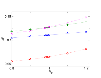
Figure 3: Energies of the four lowest excited states in the neutral sector $S^{z}=\Delta N_{c}=0$ for $U=3$, $J^{z}_{1}=V_{1}=0$ and $L=64$ as a function of $V_{2}$. The critical value $V_{2}^{c}$ is identified through the crossing of the two nearly degenerate states in the $(2s,0)$ multiplet. Lines are guide to the eye.

Next, we vary $V_{1}$ and $J_{1}^{z}$ to bring $K_{c}$ and $K_{s}$ close to $1/2$. After searching in parameter space, we settle for the particular parameter set

$$U=3\ ,\ V_{1}=0.85\ ,\ V_{2}=1.1\ ,\ J_{1}^{z}=5.2.$$ (171)

The analysis presented below suggests that this corresponds to Luttinger parameter values of $K_{s}=0.655$ and $K_{c}=0.500$. This is probably as close to the LE point as one can get without a more precise theoretical description of finite-size energies based on a renormalization-group-improved perturbation theory analysis.

Figure 4 shows numerical results for the quantity $\delta(L)$ defined in Eq. (166).

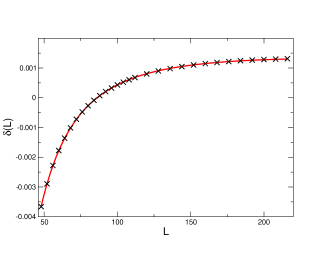
Figure 4: Crosses: numerical results for $\delta(L)$ as defined in Eq. (166). The solid line is the best fit to Eq. (167) and is obtained for $K_{s}=0.655,\tilde{a}_{1}=0.009$, $\tilde{b}_{1}=0.493$ and $\tilde{b}_{2}=-5.131$.

The data have been fitted using (167). The resulting best-fit estimates are

$$K_{s}=0.655,$$ (172)

$\tilde{a}_{1}=0.009$, $\tilde{b}_{1}=0.493$ and $\tilde{b}_{2}=-5.131$. The quality of the fit is visibly excellent (the residuals are $\sim 10^{-6}$). The numerical value for $\tilde{a}_{1}$ is very small, confirming that we have almost succeeded with fine-tuning the spinon mass term to zero (on the scale set by the system sizes we consider).

In the next step we determine the spin velocity using (165) and retaining the $b_{1}$ and $b_{2}$ terms. Setting $K_{s}=0.655$ we obtain

$$v_{s}\approx 1.707.$$ (173)

This value is consistent with the result obtained by considering $\Delta E(0,0,\{m_{\ell}^{s}=\delta_{\ell,1},m^{c}_{\ell}=0\})$ in Eq. (168). We have verified that the energy level corresponds to the first spin descendant state by tracking the tower of lowest-lying energies in the neutral sector along a path in parameter space connecting the Hubbard model to the point (171).

Having determined $v_{s}$ and $K_{s}$, we now turn to the charge sector. In Fig. 5 we present numerical results for the quantity $f(L)$ defined in Eq. (170), together with a fit to the functional form posited in (170). The spin Luttinger parameter is fixed as $K_{s}=0.655$. The best-fit estimates are

$$\frac{\pi v_{c}}{8K_{c}}=2.000,$$ (174)

and $b_{2}^{c}=0.271$. The residuals are of order $\mathcal{O}(10^{-5})$.

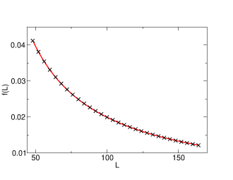
Figure 5: Crosses: numerical results for $f(L)$ as defined in (170). The solid line is a best fit to (170) with $K_{s}=0.655$.

Finally, in Fig. 6 we present numerical results for $\Delta E(0,0,\{m_{\ell}^{s}=0,m^{c}_{\ell}=\delta_{\ell,1}\})$. Fitting the data to (169) with $K_{s}=0.655$ results in estimates

$$v_{c}\approx 2.543,$$ (175)

and $\tilde{b}_{2}^{c}=-1.191$. Combining (174) and (175) we conclude that

$$K_{c}\approx 0.500.$$ (176)

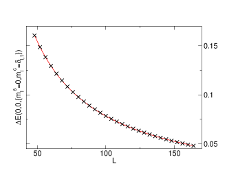
Figure 6: Crosses: numerical results for $\Delta E(0,0,\{m_{\ell}^{s}=0,m^{c}_{\ell}=\delta_{\ell,1}\})$. The solid line is a best fit to (169) for $K_{s}=0.655$.

VII.6 Friedel oscillations

The analysis of finite-size energy levels presented above is clearly rather involved, and an independent check on the results for $K_{c,s}$ would clearly be very useful. Such a check is provided by analyzing Friedel oscillations of the charge density on a chain with open boundary conditions, cf Ref. soeffing2009, . We summarize the main steps of how to calculate the charge density for open boundary conditions in (perturbed) Luttinger liquid theory in Appendix D. For a quarter filled band we obtain

$$n_{j} \approx \frac{1}{2}+\frac{d_{1}}{(D_{j})^{2K_{s}}}+d_{2}\frac{\sin\big{(}\big{[}\frac{\pi}{2}+\frac{p_{1}}{L+1}\big{]}j+p_{2}\big{)}}{(D_{j})^{(K_{c}+K_{s})/2}}$$ (177)

$$+d_{3}\frac{\cos\big{(}\big{[}\pi+\frac{2p_{1}}{L+1}\big{]}j+2p_{2}\big{)}}{(D_{j})^{2K_{c}}}+\ldots,$$

where $D_{j}$ denotes

$$D_{j}=\frac{2(L+1)}{\pi}\sin\big{(}\frac{\pi j}{L+1}\big{)}.$$ (178)

In Fig. 7 we compare the prediction (177) to DMRG results for a quarter filled band and system size $L=208$. We fix the values of the Luttinger parameters to $K_{s}=0.65$ and $K_{c}=0.5$ and use the amplitudes $d_{j}$ and phase shifts $p_{j}$ as fit parameters. The agreement is very good except near the boundaries. The best fit is obtained for $d_{1}=-0.05$, $d_{2}=0.83$, $d_{3}=0.01$, $p_{1}=-\pi/4$ and $p_{2}=-\pi/2$.

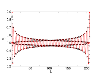
Figure 7: Crosses: local density for a quarter filled band and $U=3$, $V_{1}=0.85$, $V_{2}=1.1$, $J_{1}^{z}=5.2$. The solid line is a fit to eqn (177) with $K_{s}=0.65$ and $K_{c}=0.5$.

The good agreement between the expected behaviour (177) and the DMRG results provides a consistency check on the values of $K_{c,s}$ extracted from the analysis of finite-size energy levels.

VIII Summary and Conclusions

In this work we have developed a new approach to deriving mobile impurity models for studying dynamical correlations in gapless models of spinful fermions. Our construction is based on the principle that our mobile impurity must carry the quantum numbers of a holon/antiholon (charge $\pm e$, spin $0$) or a spinon (charge $0$ and spin $\pm 1/2$). For the case of integrable models like the Hubbard chain, it is known from the exact solution that elementary excitations at finite energies are (anti)holons and spinons with precisely these quantum numbers. In integrable models these excitations are stable (i.e. do not decay). Breaking integrability is expected to render their lifetimes finite, but leaving their spin and charge quantum numbers intact.

To facilitate our construction, we first derived a representation of spinful nonlinear Luttinger liquids in terms of strongly interacting fermionic holons and spinons. At a particular Luther-Emery point for spin and charge, holons and spinons become noninteracting. Using this as our point of reference, we derived a mobile impurity model appropriate for the description of threshold singularities in the single-particle spectral function for a general class of extended Hubbard models in their Luttinger liquid phase.

Our construction differs in important aspects from previous work by Schmidt, Imambekov and GlazmanSIG1 ; SIG2 . However, we demonstrated explicitly how and why results for threshold exponents obtained in the two approaches coincide.

Finally, we presented a preliminary analysis of the question of how to realize, in the low-energy regime, the Luther-Emery point for spin and charge in a lattice model of interacting spinful fermions. We showed that the structure of allowed perturbations to the Luther-Emery point is such that fine tunings of various interactions is required. Achieving these fine tunings is very delicate, and we discussed in some detail what problems one encounters.

Our work raises a number of interesting questions that deserve further attention. First and foremost, further numerical studies are required in order to identify a parameter regime in an appropriate extended Hubbard model that, at least approximately, realizes the Luther-Emery point. Second, it would be very interesting to implement the numerical procedure we proposed for determining the parameters $\gamma_{\alpha}$, $\bar{\gamma}_{\alpha}$ characterizing the threshold exponents. One first might want to reproduce the known exact results for the Hubbard model, before moving on to non-integrable cases. Third, in close proximity to the Luther-Emery point the mobile impurity model involves an additional marginal interaction that cannot be removed by a unitary transformation. It would be interesting to analyze its effects on the threshold exponents.

Appendix A Irrelevant perturbations to the Luttinger liquid Hamiltonian

One way of working out the allowed irrelevant perturbations to the Luttinger liquid Hamiltonian is by using symmetry considerations. Our starting point are extended Hubbard models of the kind (53). For the purposes of this appendix, we will assume all interactions to be small.

A.1 Symmetries

Our lattice models of interest are invariant under various symmetry operations. These symmetries are inherited by the bosonic low-energy description (60) and we now discuss their realizations.

A.1.1 Spin flip symmetry

The lattice models of interest are invariant under exchange of up and down spins

$$c_{j,\uparrow}\leftrightarrow c_{j,\downarrow}.$$ (179)

is realized at the level of the bosonic fields as

$$\begin{pmatrix}\varphi_{s}(x)\\ \bar{\varphi}_{s}(x)\\ \eta_{\uparrow}\\ \bar{\eta}_{\uparrow}\end{pmatrix}\longrightarrow-\begin{pmatrix}\varphi_{s}(x)\\ \bar{\varphi}_{s}(x)\\ \eta_{\downarrow}\\ \bar{\eta}_{\downarrow}\end{pmatrix}.$$ (180)

A.1.2 Translational Invariance:

The translation operator acts as

$$T^{\dagger}c_{j,\sigma}T=c_{j+1,\sigma}.$$ (181)

We can implement this on the level of bosonic fields by imposing the transformation properties

$$\begin{pmatrix}\varphi_{c}(x)\\ \bar{\varphi}_{c}(x)\end{pmatrix} \longrightarrow \begin{pmatrix}\varphi_{c}(x)-2k_{F}a_{0}\\ \bar{\varphi}_{c}(x)-2k_{F}a_{0}\end{pmatrix}\ ,$$

$$\begin{pmatrix}\varphi_{s}(x)\\ \bar{\varphi}_{s}(x)\end{pmatrix} \longrightarrow \begin{pmatrix}\varphi_{s}(x)\\ \bar{\varphi}_{s}(x)\end{pmatrix}.$$ (182)

We note that this transformation works for all higher harmonics in (54). Translational invariance of the Hamiltonian then implies that it generically may not contain any vertex operators of the charge boson. Exceptions to this rule occur at commensurate fillings

$$k_{F}a_{0}=\pi\frac{p}{q}\ ,\quad p,q\in\mathbb{N}.$$ (183)

Here operators of the form

$$\cos\big{(}\frac{q}{2}\Phi_{c}\big{)}\ ,\quad\sin\big{(}\frac{q}{2}\Phi_{c}\big{)}$$ (184)

are allowed to occur. As long as $q>4$ such operators are highly irrelevant and do not play a role in the following discussion.

A.1.3 $U(1)\otimes U(1)$ Invariance

By this mean we that the Hamiltonian commutes with particle number and the z-component of total spin

$$[H,\hat{S}^{z}]=[H,\hat{N}]=0.$$ (185)

This symmetry implies that no vertex operators involving the dual fields $\Theta_{c}$, $\Theta_{s}$ are allowed to occur in the expression for ${\cal H}$.

A.1.4 Site Parity

The reflection symmetry acts on the lattice fermion operators like

$$Pc_{j,\sigma}P=c_{-j,\sigma}.$$ (186)

We see that $P$ can be realized in the field theory as

$$P\varphi_{a}(x)P = -\bar{\varphi}_{a}(-x)\ ,\quad P\bar{\varphi}_{a}(x)P=-{\varphi}_{a}(-x)\ ,$$

$$P\eta_{\sigma}P = \bar{\eta}_{\sigma}.$$ (187)

Crucially, parity acts on the unphysical Klein degrees of freedom as well. Moreover, we obtain the following constraints on the amplitudes $A_{n,m}$ in (54)

$$A_{n,m}=A_{1-n,-1-m}.$$ (188)

A.2 Dimension two operators allowed by symmetry

We now list all symmetry-allowed perturbations to the Luttinger liquid Hamiltonian for noninteracting spinful fermions with scaling dimensions $2$, $3$ and $4$. Such perturbations will be of the form

$$\sum_{j}\hat{\Gamma}_{j}\lambda_{j}\int dx\ {\cal O}(x),$$ (189)

where $\lambda_{j}$ are coupling constants and $\Gamma_{j}$ are products of Klein factors. The only non-trivial combination of Klein factors allowed to appear is in fact

$$\eta_{\uparrow}\bar{\eta}_{\uparrow}\eta_{\downarrow}\bar{\eta}_{\downarrow}.$$ (190)

This is because the all terms in our Hamiltonian (53) are of the form

$$c^{\dagger}_{j,\sigma}c_{k,\sigma},\quad c^{\dagger}_{j,\sigma}c^{\dagger}_{k,\tau}c_{l,\tau}c_{m,\sigma}\ .$$ (191)

Expressing the lattice fermion operators in terms of Bose fields by (54), and then imposing that for a given interaction to appear in the Hamiltonian it must not contain a rapidly oscillating factor $e^{ijk_{F}x}$, one finds that the Klein factors either cancel or combine to $\eta_{\uparrow}\bar{\eta}_{\uparrow}\eta_{\downarrow}\bar{\eta}_{\downarrow}$.

Taking this into account, we find five symmetry-allowed dimension two operators

$${\cal O}^{(2)}_{1} = \cos\Phi_{s}\ ,$$

$${\cal O}^{(2)}_{2} = (\partial_{x}\varphi_{s})^{2}+(\partial_{x}\bar{\varphi}_{s})^{2}\ ,$$

$${\cal O}^{(2)}_{3} = \partial_{x}\varphi_{s}\partial_{x}\bar{\varphi}_{s}\ ,$$

$${\cal O}^{(2)}_{4} = (\partial_{x}\varphi_{c})^{2}+(\partial_{x}\bar{\varphi}_{c})^{2}\ ,$$

$${\cal O}^{(2)}_{5} = \partial_{x}\varphi_{c}\partial_{x}\bar{\varphi}_{c}\ .$$ (192)

We note that none of these leads to a coupling between spin and charge sectors. In order to see that the operator $\cos\Phi_{s}$ is allowed, but $\sin\Phi_{s}$ is not, one needs to consider the structure of Klein factors in (54).

A.3 Dimension three operators allowed by symmetry

The analogous analysis for dimension three operators gives the three possible perturbations involving only the charge sector

$${\cal O}^{(3)}_{1} = (\partial_{x}\varphi_{c})^{3}+(\partial_{x}\bar{\varphi}_{c})^{3}\ ,$$

$${\cal O}^{(3)}_{2} = (\partial_{x}\varphi_{c})^{2}\partial_{x}\bar{\varphi}_{c}+(\partial_{x}\bar{\varphi}_{c})^{2}\partial_{x}\varphi_{c}\ ,$$

$${\cal O}^{(3)}_{3} = \partial_{x}\varphi_{c}\partial^{2}_{x}\bar{\varphi}_{c}-\partial_{x}\bar{\varphi}_{c}\partial^{2}_{x}\varphi_{c},$$ (193)

and four possible perturbations that couple spin and charge sectors together

$${\cal O}^{(3)}_{4} = (\partial_{x}\varphi_{s})^{2}\partial_{x}\varphi_{c}+(\partial_{x}\bar{\varphi}_{s})^{2}\partial_{x}\bar{\varphi}_{c}\ ,$$

$${\cal O}^{(3)}_{5} = (\partial_{x}\varphi_{s})^{2}\partial_{x}\bar{\varphi}_{c}+(\partial_{x}\bar{\varphi}_{s})^{2}\partial_{x}\varphi_{c}\ ,$$

$${\cal O}^{(3)}_{6} = \partial_{x}\varphi_{s}\partial_{x}\bar{\varphi}_{s}(\partial_{x}\bar{\varphi}_{c}+\partial_{x}\varphi_{c})\ ,$$

$${\cal O}^{(3)}_{7} = \big{(}\partial_{x}\varphi_{c}+\partial_{x}\bar{\varphi}_{c}\big{)}\cos(\Phi_{s})\ .$$ (194)

A.4 Dimension four operators allowed by symmetry

Finally we consider all symmetry-allowed dimension four operators.

A.4.1 Charge sector only

We find six perturbations involving only the charge sector

$${\cal O}^{(4)}_{1} = (\partial_{x}\varphi_{c})^{4}+(\partial_{x}\bar{\varphi}_{c})^{4}\ ,$$

$${\cal O}^{(4)}_{2} = (\partial_{x}\varphi_{c})^{2}(\partial_{x}\bar{\varphi}_{c})^{2}\ ,$$

$${\cal O}^{(4)}_{3} = (\partial_{x}\varphi_{c})^{3}\partial_{x}\bar{\varphi}_{c}+(\partial_{x}\bar{\varphi}_{c})^{3}\partial_{x}\varphi_{c}\ ,$$

$${\cal O}^{(4)}_{4} = (\partial_{x}^{2}\varphi_{c})^{2}+(\partial_{x}^{2}\bar{\varphi}_{c})^{2}\ ,$$

$${\cal O}^{(4)}_{5} = \partial_{x}^{2}\varphi_{c}\partial_{x}^{2}\bar{\varphi}_{c}\ ,$$

$${\cal O}^{(4)}_{6} = \partial_{x}^{2}\varphi_{c}(\partial_{x}\bar{\varphi}_{c})^{2}-\partial_{x}^{2}\bar{\varphi}_{c}(\partial_{x}\varphi_{c})^{2}.$$ (195)

Here we have used that

$$\partial_{x}^{3}\varphi_{c}\partial_{x}\bar{\varphi}_{c}+\partial_{x}^{3}\bar{\varphi}_{c}\partial_{x}\varphi_{c} = -2\partial_{x}^{2}\varphi_{c}\partial_{x}^{2}\bar{\varphi}_{c}$$ (196)

$$+ \text{total derivative}.$$

A.4.2 Spin sector only

We find altogether eight symmetry allowed perturbations involving only the spin sector

$${\cal O}^{(4)}_{7} = (\partial_{x}\varphi_{s})^{4}+(\partial_{x}\bar{\varphi}_{s})^{4}\ ,$$

$${\cal O}^{(4)}_{8} = (\partial_{x}\varphi_{s})^{2}(\partial_{x}\bar{\varphi}_{s})^{2}\ ,$$

$${\cal O}^{(4)}_{9} = (\partial_{x}\varphi_{s})^{3}\partial_{x}\bar{\varphi}_{s}+(\partial_{x}\bar{\varphi}_{s})^{3}\partial_{x}\varphi_{s}\ ,$$

$${\cal O}^{(4)}_{10} = (\partial_{x}^{2}\varphi_{s})^{2}+(\partial_{x}^{2}\bar{\varphi}_{s})^{2}\ ,$$

$${\cal O}^{(4)}_{11} = \partial_{x}^{2}\varphi_{s}\partial_{x}^{2}\bar{\varphi}_{s}\ ,$$

$${\cal O}^{(4)}_{12} = \cos(\Phi_{s})\partial_{x}\varphi_{s}\partial_{x}\bar{\varphi}_{s}\ ,$$

$${\cal O}^{(4)}_{13} = \cos(\Phi_{s})\left[(\partial_{x}\varphi_{s})^{2}+(\partial_{x}\bar{\varphi}_{s})^{2}\right].$$ (197)

A.4.3 Terms coupling charge and spin

Finally, there are eight symmetry-allowed perturbations involving both spin and charge sectors

$${\cal O}^{(4)}_{15} = \cos(\Phi_{s})\partial_{x}\varphi_{c}\partial_{x}\bar{\varphi}_{c}\ ,$$

$${\cal O}^{(4)}_{16} = \cos(\Phi_{s})\left[(\partial_{x}\varphi_{c})^{2}+(\partial_{x}\bar{\varphi}_{c})^{2}\right],$$

$${\cal O}^{(4)}_{17} = [(\partial_{x}\varphi_{s})^{2}+(\partial_{x}\bar{\varphi}_{s})^{2}][(\partial_{x}\varphi_{c})^{2}+(\partial_{x}\bar{\varphi}_{c})^{2}],$$

$${\cal O}^{(4)}_{18} = [(\partial_{x}\varphi_{s})^{2}+(\partial_{x}\bar{\varphi}_{s})^{2}]\partial_{x}\varphi_{c}\partial_{x}\bar{\varphi}_{c},$$

$${\cal O}^{(4)}_{19} = \partial_{x}\varphi_{s}\partial_{x}\bar{\varphi}_{s}[(\partial_{x}\varphi_{c})^{2}+(\partial_{x}\bar{\varphi}_{c})^{2}],$$

$${\cal O}^{(4)}_{20} = \partial_{x}\varphi_{s}\partial_{x}\bar{\varphi}_{s}\ \partial_{x}\varphi_{c}\partial_{x}\bar{\varphi}_{c},$$

$${\cal O}^{(4)}_{21} = [(\partial_{x}\varphi_{s})^{2}+(\partial_{x}\bar{\varphi}_{s})^{2}]\ [\partial_{x}^{2}\varphi_{c}-\partial_{x}^{2}\bar{\varphi}_{c}],$$

$${\cal O}^{(4)}_{22} = \partial_{x}\varphi_{s}\partial_{x}\bar{\varphi}_{s}\ [\partial_{x}^{2}\varphi_{c}-\partial_{x}^{2}\bar{\varphi}_{c}].$$ (198)

Appendix B List of irrelevant operators at the LE point

The symmetries of the Hamiltonian at the Luther-Emery point are the same as those listed in Sec. A. Since at the LE point all symmetry-allowed operators in the Hamiltonian are local in terms of free holons and spinons, we shall give the list of irrelevant operators directly in the fermionic representation. Among the operators listed in Appendix A, those which involve only derivatives of $\varphi_{\alpha},\bar{\varphi}_{\alpha}$ preserve the same scaling dimension at the LE point; their expressions in the fermionic basis can be obtained straightforwardly by using bosonization identities for spinless fermions.

On the other hand, operators that contain $\cos(\Phi_{s})$ require a more careful analysis. First we note that, taking into account the Klein factors, the operator is actually represented by

$$\cos(\Phi_{s})\to\eta_{\uparrow}\bar{\eta}_{\downarrow}\eta_{\downarrow}\bar{\eta}_{\uparrow}\cos(\Phi_{s}).$$ (199)

Recall that spin flip and parity act nontrivially on $\eta_{\sigma},\bar{\eta}_{\sigma}$. However, the product of four Majorana fermions in Eq. (199) is invariant under both transformations. As a result, the Klein factors can be safely omitted in the symmetry analysis of the bosonized perturbations to the Luttinger model. At the LE point, however, $\cos(\Phi_{s})$ must be refermionized into free spinons according to Eq. (73). In terms of spinon operators, spin-flip symmetry is equivalent to a particle-hole symmetry

$$R^{\phantom{\dagger}}_{s}\leftrightarrow R_{s}^{\dagger},\quad L^{\phantom{\dagger}}_{s}\leftrightarrow L_{s}^{\dagger},$$ (200)

while leaving the spinon Klein factors $\eta_{s},\bar{\eta}_{s}$ invariant. Parity acts on spinon operators in the form

$$PR_{s}(x)P = L_{s}(-x),\quad PL_{s}(x)P=R_{s}(-x),$$ (201)

$$P\eta_{s}P = \bar{\eta}_{s},\quad P\bar{\eta}_{s}P=\eta_{s}.$$ (202)

The refermionization of $\cos(\Phi_{s})$ at the LE point yields

$$\cos(\Phi_{s}) \to \cos(\Phi_{s}^{*}/\sqrt{2})$$ (203)

$$\sim \pi(\eta_{s}R_{s}^{\dagger}\bar{\eta}_{s}L^{\phantom{\dagger}}_{s}+\eta_{s}R_{s}^{\phantom{\dagger}}\bar{\eta}_{s}L^{\dagger}_{s})$$

$$= -\pi(\eta_{s}\bar{\eta}_{s}R_{s}^{\dagger}L^{\phantom{\dagger}}_{s}+\bar{\eta}_{s}\eta_{s}L^{\dagger}_{s}R_{s}^{\phantom{\dagger}}).$$

Notice that the operator in Eq. (203) is invariant under the spin-flip transformation (200) only if we take the spinon Klein factors into account explicitly. Nevertheless, in the following list of irrelevant operators we shall omit the Klein factors for short and write simply

$$\cos(\Phi_{s})\to(R_{s}^{\dagger}L^{\phantom{\dagger}}_{s}+L^{\dagger}_{s}R_{s}^{\phantom{\dagger}}).$$ (204)

Since all the operators that stem from $\cos(\Phi_{s})$ contain the same combination of Klein factors in Eq. (203), we can adopt the prescription in Eq. (204) supplemented by the ad hoc rule that spin-flip symmetry takes $R^{\phantom{\dagger}}_{s}\to R^{\dagger}_{s}$ but $L^{\phantom{\dagger}}_{s}\to-L^{\dagger}_{s}$.

Importantly, the operator $\cos(\Phi_{s})$ has scaling dimension 2 at the SU(2)-symmetric weak coupling regime, but dimension 1 at the LE point. Therefore, the scaling dimension of perturbations that contain $\cos(\Phi_{s})$ is reduced by 1 as we go from weak coupling to the LE point. For instance, the marginal operator $\mathcal{O}^{(2)}_{1}=\cos(\Phi_{s})$ at the SU(2) point becomes the relevant mass term of the Thirring model, $\cos(\Phi_{s}^{*}/\sqrt{2})\sim R_{s}^{\dagger}L^{\phantom{\dagger}}_{s}+L_{s}^{\dagger}R^{\phantom{\dagger}}_{s}$ at the LE point, while the irrelevant (dimension-three) operator $\mathcal{O}_{7}^{(3)}=(\partial_{x}\bar{\varphi}_{c}+\partial_{x}\varphi_{c})\cos(\Phi_{s})$ at the SU(2) point gives rise to the marginal spin-charge coupling $(R_{s}^{\dagger}L^{\phantom{\dagger}}_{s}+L_{s}^{\dagger}R^{\phantom{\dagger}}_{s})(R_{c}^{\dagger}R^{\phantom{\dagger}}_{c}+L_{c}^{\dagger}L^{\phantom{\dagger}}_{c})$ at the LE point. This implies that, in order to have the complete list of irrelevant operators up to dimension four at the LE point, we have to consider the refermionization of operators that have dimension 5 at the SU(2) point and were not included in the list in Appendix A. The latter correspond to operators $\mathcal{V}^{(4)}_{21}$ through $\mathcal{V}^{(4)}_{27}$ in the list below.

B.1 Dimension-three operators allowed by symmetry

$$\mathcal{V}_{1}^{(3)} = R_{c}^{\dagger}\partial_{x}^{2}R_{c}^{\phantom{\dagger}}+L_{c}^{\dagger}\partial_{x}^{2}L_{c}^{\phantom{\dagger}}+\text{h.c.},$$ (205)

$$\mathcal{V}_{2}^{(3)} = R_{c}^{\dagger}R_{c}^{\phantom{\dagger}}L_{c}^{\dagger}i\partial_{x}L_{c}^{\phantom{\dagger}}-L_{c}^{\dagger}L_{c}^{\phantom{\dagger}}R_{c}^{\dagger}i\partial_{x}R_{c}^{\phantom{\dagger}}+\text{h.c.}.$$ (206)

$$\mathcal{V}_{3}^{(3)} = \partial_{x}(R_{c}^{\dagger}R_{c}^{\phantom{\dagger}})L_{c}^{\dagger}L_{c}^{\phantom{\dagger}}-\partial_{x}(L_{c}^{\dagger}L_{c}^{\phantom{\dagger}})R_{c}^{\dagger}R_{c}^{\phantom{\dagger}},$$ (207)

$$\mathcal{V}_{4}^{(3)} = \partial_{x}R_{s}^{\dagger}\partial_{x}L_{s}^{\phantom{\dagger}}+\partial_{x}L_{s}^{\dagger}\partial_{x}R_{s}^{\phantom{\dagger}},$$ (208)

$$\mathcal{V}_{5}^{(3)} = iR_{s}^{\dagger}\partial_{x}R_{s}^{\phantom{\dagger}}L_{s}^{\dagger}R_{s}^{\phantom{\dagger}}-iL_{s}^{\dagger}\partial_{x}L_{s}^{\phantom{\dagger}}R_{s}^{\dagger}L_{s}^{\phantom{\dagger}}+\text{h.c.},$$ (209)

$$\mathcal{V}_{6}^{(3)} = R_{c}^{\dagger}R_{c}^{\phantom{\dagger}}R_{s}^{\dagger}i\partial_{x}R_{s}^{\phantom{\dagger}}-L_{c}^{\dagger}L_{c}^{\phantom{\dagger}}L_{s}^{\dagger}i\partial_{x}L_{s}^{\phantom{\dagger}}+\text{h.c.},$$ (210)

$$\mathcal{V}_{7}^{(3)} = R_{c}^{\dagger}R_{c}^{\phantom{\dagger}}L_{s}^{\dagger}i\partial_{x}L_{s}^{\phantom{\dagger}}-L_{c}^{\dagger}L_{c}^{\phantom{\dagger}}R_{s}^{\dagger}i\partial_{x}R_{s}^{\phantom{\dagger}}+\text{h.c.},$$ (211)

$$\mathcal{V}_{8}^{(3)} = (R_{c}^{\dagger}R_{c}^{\phantom{\dagger}}+L_{c}^{\dagger}L_{c}^{\phantom{\dagger}})R_{s}^{\dagger}R_{s}^{\phantom{\dagger}}L_{s}^{\dagger}L_{s}^{\phantom{\dagger}},$$ (212)

$$\mathcal{V}_{9}^{(3)} = (iR_{c}^{\dagger}\partial_{x}R_{c}^{\phantom{\dagger}}-iL_{c}^{\dagger}\partial_{x}L_{c}^{\phantom{\dagger}}+\text{h.c.})$$ (213)

$$\times(R_{s}^{\dagger}L_{s}^{\phantom{\dagger}}+L_{s}^{\dagger}R_{s}^{\phantom{\dagger}}),$$

$$\mathcal{V}_{10}^{(3)} = R_{c}^{\dagger}R_{c}^{\phantom{\dagger}}L_{c}^{\dagger}L_{c}^{\phantom{\dagger}}(R_{s}^{\dagger}L_{s}^{\phantom{\dagger}}+L_{s}^{\dagger}R_{s}^{\phantom{\dagger}}),$$ (214)

$$\mathcal{V}_{11}^{(3)} = \partial_{x}(R_{c}^{\dagger}R_{c}^{\phantom{\dagger}}-L_{c}^{\dagger}L_{c}^{\phantom{\dagger}})(R_{s}^{\dagger}L_{s}^{\phantom{\dagger}}+L_{s}^{\dagger}R_{s}^{\phantom{\dagger}}).$$ (215)

B.2 Dimension-four operators allowed by symmetry

B.2.1 Charge sector only

$$\mathcal{V}^{(4)}_{1} = iR_{c}^{\dagger}\partial_{x}^{3}R_{c}^{\phantom{\dagger}}-iL_{c}^{\dagger}\partial_{x}^{3}L_{c}^{\phantom{\dagger}}+\text{h.c.},$$ (216)

$$\mathcal{V}^{(4)}_{2} = R_{c}^{\dagger}\partial_{x}R_{c}^{\phantom{\dagger}}L_{c}^{\dagger}\partial_{x}L_{c}^{\phantom{\dagger}}+\text{h.c.},$$ (217)

$$\mathcal{V}^{(4)}_{3} = R_{c}^{\dagger}\partial^{2}_{x}R_{c}^{\phantom{\dagger}}L_{c}^{\dagger}L_{c}^{\phantom{\dagger}}+L_{c}^{\dagger}\partial^{2}_{x}L_{c}^{\phantom{\dagger}}R_{c}^{\dagger}R_{c}^{\phantom{\dagger}}+\text{h.c.},$$ (218)

$$\mathcal{V}^{(4)}_{4} = R_{c}^{\dagger}\partial_{x}R_{c}^{\dagger}R_{c}^{\phantom{\dagger}}\partial_{x}R_{c}^{\phantom{\dagger}}+L_{c}^{\dagger}\partial_{x}L_{c}^{\dagger}L_{c}^{\phantom{\dagger}}\partial_{x}L_{c}^{\phantom{\dagger}},$$ (219)

$$\mathcal{V}^{(4)}_{5} = \partial_{x}(R_{c}^{\dagger}R_{c}^{\phantom{\dagger}})\partial_{x}(L_{c}^{\dagger}L_{c}^{\phantom{\dagger}}),$$ (220)

$$\mathcal{V}^{(4)}_{6} = \partial_{x}(R_{c}^{\dagger}R_{c}^{\phantom{\dagger}})L_{c}^{\dagger}i\partial_{x}L_{c}^{\phantom{\dagger}}+\partial_{x}(L_{c}^{\dagger}L_{c}^{\phantom{\dagger}})R_{c}^{\dagger}i\partial_{x}R_{c}^{\phantom{\dagger}}$$ (221)

$$+\text{h.c.}.$$

B.2.2 Spin sector only

$$\mathcal{V}^{(4)}_{7} = iR_{s}^{\dagger}\partial_{x}^{3}R_{s}^{\phantom{\dagger}}-iL_{s}^{\dagger}\partial_{x}^{3}L_{s}^{\phantom{\dagger}},$$ (222)

$$\mathcal{V}^{(4)}_{8} = R_{s}^{\dagger}\partial_{x}R_{s}^{\phantom{\dagger}}L_{s}^{\dagger}\partial_{x}L_{s}^{\phantom{\dagger}}+\text{h.c.},$$ (223)

$$\mathcal{V}^{(4)}_{9} = R_{s}^{\dagger}\partial_{x}R_{s}^{\dagger}L_{s}^{\phantom{\dagger}}\partial_{x}L_{s}^{\phantom{\dagger}}+L_{s}^{\dagger}\partial_{x}L_{s}^{\dagger}R_{s}^{\phantom{\dagger}}\partial_{x}R_{s}^{\phantom{\dagger}},$$ (224)

$$\mathcal{V}^{(4)}_{10} = R_{s}^{\dagger}\partial_{x}^{2}R_{s}^{\phantom{\dagger}}L_{s}^{\dagger}L_{s}^{\phantom{\dagger}}+L_{s}^{\dagger}\partial_{x}^{2}L_{s}^{\phantom{\dagger}}R_{s}^{\dagger}R_{s}^{\phantom{\dagger}}+\text{h.c.},$$ (225)

$$\mathcal{V}^{(4)}_{11} = R_{s}^{\dagger}\partial_{x}R_{s}^{\dagger}R_{s}^{\phantom{\dagger}}\partial_{x}R_{s}^{\phantom{\dagger}}+L_{s}^{\dagger}\partial_{x}L_{s}^{\dagger}L_{s}^{\phantom{\dagger}}\partial_{x}L_{s}^{\phantom{\dagger}},$$ (226)

$$\mathcal{V}^{(4)}_{12} = \partial_{x}(R_{s}^{\dagger}R_{s}^{\phantom{\dagger}})\partial_{x}(L_{s}^{\dagger}L_{s}^{\phantom{\dagger}}).$$ (227)

B.2.3 Terms coupling charge and spin

$$\mathcal{V}^{(4)}_{13} = (iR_{c}^{\dagger}\partial_{x}R_{c}^{\phantom{\dagger}}+\text{h.c.})(iR_{s}^{\dagger}\partial_{x}R_{s}^{\phantom{\dagger}}+\text{h.c.})$$ (228)

$$+(iL_{c}^{\dagger}\partial_{x}L_{c}^{\phantom{\dagger}}+\text{h.c.})(iL_{s}^{\dagger}\partial_{x}L_{s}^{\phantom{\dagger}}+\text{h.c.}),$$

$$\mathcal{V}^{(4)}_{14} = (iR_{c}^{\dagger}\partial_{x}R_{c}^{\phantom{\dagger}}+\text{h.c.})(iL_{s}^{\dagger}\partial_{x}L_{s}^{\phantom{\dagger}}+\text{h.c.})$$ (229)

$$+(iL_{c}^{\dagger}\partial_{x}L_{c}^{\phantom{\dagger}}+\text{h.c.})(iR_{s}^{\dagger}\partial_{x}R_{s}^{\phantom{\dagger}}+\text{h.c.}),$$

$$\mathcal{V}^{(4)}_{15} = R_{c}^{\dagger}R_{c}^{\phantom{\dagger}}L_{c}^{\dagger}L_{c}^{\phantom{\dagger}}(iR_{s}^{\dagger}\partial_{x}R_{s}^{\phantom{\dagger}}-iL_{s}^{\dagger}\partial_{x}L_{s}^{\phantom{\dagger}}+\text{h.c.}),$$ (230)

$$\mathcal{V}^{(4)}_{16} = (iR_{c}^{\dagger}\partial_{x}R_{c}^{\phantom{\dagger}}-iL_{c}^{\dagger}\partial_{x}L_{c}^{\phantom{\dagger}}+\text{h.c.})R_{s}^{\dagger}R_{s}^{\phantom{\dagger}}L_{s}^{\dagger}L_{s}^{\phantom{\dagger}},$$ (231)

$$\mathcal{V}^{(4)}_{17} = R_{c}^{\dagger}R_{c}^{\phantom{\dagger}}L_{c}^{\dagger}L_{c}^{\phantom{\dagger}}R_{s}^{\dagger}R_{s}^{\phantom{\dagger}}L_{s}^{\dagger}L_{s}^{\phantom{\dagger}},$$ (232)

$$\mathcal{V}^{(4)}_{18} = \partial_{x}(R_{c}^{\dagger}R_{c}^{\phantom{\dagger}})(iR_{s}^{\dagger}\partial_{x}R_{s}^{\phantom{\dagger}}+\text{h.c.})$$ (233)

$$+\partial_{x}(L_{c}^{\dagger}L_{c}^{\phantom{\dagger}})(iL_{s}^{\dagger}\partial_{x}L_{s}^{\phantom{\dagger}}+\text{h.c.}),$$

$$\mathcal{V}^{(4)}_{19} = \partial_{x}(R_{c}^{\dagger}R_{c}^{\phantom{\dagger}})(iL_{s}^{\dagger}\partial_{x}L_{s}^{\phantom{\dagger}}+\text{h.c.})$$ (234)

$$+\partial_{x}(L_{c}^{\dagger}L_{c}^{\phantom{\dagger}})(iR_{s}^{\dagger}\partial_{x}R_{s}^{\phantom{\dagger}}+\text{h.c.}),$$

$$\mathcal{V}^{(4)}_{20} = \partial_{x}(R_{c}^{\dagger}R_{c}^{\phantom{\dagger}}-L_{c}^{\dagger}L_{c}^{\phantom{\dagger}})R_{s}^{\dagger}R_{s}^{\phantom{\dagger}}L_{s}^{\dagger}L_{s}^{\phantom{\dagger}},$$ (235)

$$\mathcal{V}^{(4)}_{21} = (R_{c}^{\dagger}\partial_{x}^{2}R_{c}^{\phantom{\dagger}}+L_{c}^{\dagger}\partial_{x}^{2}L_{c}^{\phantom{\dagger}}+\text{h.c.})$$ (236)

$$\times(R_{s}^{\dagger}L_{s}^{\phantom{\dagger}}+L_{s}^{\dagger}R_{s}^{\phantom{\dagger}}),$$

$$\mathcal{V}^{(4)}_{22} = (R_{c}^{\dagger}R_{c}^{\phantom{\dagger}}L_{c}^{\dagger}i\partial_{x}L_{c}^{\phantom{\dagger}}-L_{c}^{\dagger}L_{c}^{\phantom{\dagger}}R_{c}^{\dagger}i\partial_{x}R_{c}^{\phantom{\dagger}}+\text{h.c.})$$ (237)

$$\times(R_{s}^{\dagger}L_{s}^{\phantom{\dagger}}+L_{s}^{\dagger}R_{s}^{\phantom{\dagger}})$$

$$\mathcal{V}^{(4)}_{23} = R_{c}^{\dagger}R_{c}^{\phantom{\dagger}}R_{s}^{\dagger}i\partial_{x}R_{s}^{\phantom{\dagger}}L_{s}^{\dagger}R_{s}^{\phantom{\dagger}}$$ (238)

$$-L_{c}^{\dagger}L_{c}^{\phantom{\dagger}}L_{s}^{\dagger}i\partial_{x}L_{s}^{\phantom{\dagger}}R_{s}^{\dagger}L_{s}^{\phantom{\dagger}}+\text{h.c.},$$

$$\mathcal{V}^{(4)}_{24} = R_{c}^{\dagger}R_{c}^{\phantom{\dagger}}L_{s}^{\dagger}i\partial_{x}L_{s}^{\phantom{\dagger}}R_{s}^{\dagger}L_{s}^{\phantom{\dagger}}$$ (239)

$$-L_{c}^{\dagger}L_{c}^{\phantom{\dagger}}R_{s}^{\dagger}i\partial_{x}R_{s}^{\phantom{\dagger}}L_{s}^{\dagger}R_{s}^{\phantom{\dagger}}+\text{h.c.}$$

$$\mathcal{V}^{(4)}_{25} = \partial_{x}^{2}(R^{\dagger}_{c}R_{c}^{\phantom{\dagger}}+L^{\dagger}_{c}L_{c}^{\phantom{\dagger}})(R^{\dagger}_{s}L_{s}^{\phantom{\dagger}}+L_{s}^{\dagger}R_{s}^{\phantom{\dagger}}),$$ (240)

$$\mathcal{V}^{(4)}_{26} = \partial_{x}(R^{\dagger}_{c}i\partial_{x}R_{c}^{\phantom{\dagger}}+L^{\dagger}_{c}i\partial_{x}L_{c}^{\phantom{\dagger}})(R^{\dagger}_{s}L_{s}^{\phantom{\dagger}}+L_{s}^{\dagger}R_{s}^{\phantom{\dagger}}),$$ (241)

$$\mathcal{V}^{(4)}_{27} = [\partial_{x}(R_{c}^{\dagger}R_{c}^{\phantom{\dagger}})L_{c}^{\dagger}L_{c}^{\phantom{\dagger}}-\partial_{x}(L_{c}^{\dagger}L_{c}^{\phantom{\dagger}})R_{c}^{\dagger}R_{c}^{\phantom{\dagger}}]$$ (242)

$$\times(R^{\dagger}_{s}L_{s}^{\phantom{\dagger}}+L_{s}^{\dagger}R_{s}^{\phantom{\dagger}}).$$

Appendix C Constraining the mobile impurity model in the SU(2)-symmetric case

We can impose SU(2) symmetry in the parameters of the mobile impurity model of Section V by requiring that the edge exponents of longitudinal and transverse spin-spin correlations coincidework7 . First consider the longitudinal component of the spin density operator:

$$S^{z}(x) \sim R_{\uparrow}^{\dagger}(x)R_{\uparrow}^{\phantom{\dagger}}(x)-R_{\downarrow}^{\dagger}(x)R_{\downarrow}^{\phantom{\dagger}}(x)$$ (243)

$$\sim \mathcal{O}_{s}^{\dagger}(x)\mathcal{O}_{s}^{\phantom{\dagger}}(x),$$

where the charge strings are cancelled in the sense of the lowest order in the OPE. We then project $\mathcal{O}_{s}(x)$ so as to create a high-energy spinon:

$$\mathcal{O}_{s}(x)\sim e^{-iqx}\chi_{s}^{\dagger}(x)e^{\frac{i}{4\sqrt{2}}\Phi_{s}^{*}(x)},$$ (244)

while $\mathcal{O}_{s}^{\dagger}(x)$ acts only in the low-energy subband:

$$\mathcal{O}_{s}^{\dagger}(x)\sim e^{\frac{i}{\sqrt{2}}\varphi_{s}^{*}-\frac{i}{4\sqrt{2}}\Phi_{s}^{*}(x)}.$$ (245)

Cancelling the neutral string, we obtain

$$S^{z}(x) \sim e^{-iqx}\chi_{s}^{\dagger}(x)e^{\frac{i}{\sqrt{2}}\varphi_{s}^{*}(x)}.$$ (246)

In terms of the transformed impurity field

$$S^{z}(x)\sim e^{-iqx}d_{s}^{\dagger}(x)e^{i\left(\frac{1}{\sqrt{2}}+\gamma_{s}\right)\varphi_{s}^{*}+i\bar{\gamma}_{s}\bar{\varphi}_{s}^{*}+i\gamma_{c}\varphi_{c}^{*}+i\bar{\gamma}_{c}\bar{\varphi}_{c}^{*}}.$$ (247)

Now, consider the transverse component:

$$S^{-}(x) \sim R^{\dagger}_{\downarrow}(x)R^{\phantom{\dagger}}_{\uparrow}(x)$$ (248)

$$\sim \mathcal{O}_{s}(x)\mathcal{O}_{s}(x)$$

$$\sim e^{-iqx}\chi_{s}^{\dagger}(x)e^{-\frac{i}{2\sqrt{2}}\varphi_{s}^{*}(x)+\frac{i}{2\sqrt{2}}\bar{\varphi}_{s}^{*}(x)}$$

$$= e^{-iqx}d_{s}^{\dagger}(x)e^{-i\left(\frac{1}{2\sqrt{2}}-\gamma_{s}\right)\varphi_{s}^{*}+i\left(\frac{1}{2\sqrt{2}}+\bar{\gamma}_{s}\right)\varphi_{s}^{*}}$$

$$\ \times e^{i\gamma_{c}\varphi_{c}^{*}+i\bar{\gamma}_{c}\bar{\varphi}_{c}^{*}}.$$

Given the expressions (247) and (248) we can calculate threshold exponents in the Fourier transforms of the spin correlations functions $\langle S^{z}(x,t)S^{z}(0,0)\rangle$ and $\langle S^{+}(x,t)S^{-}(0,0)\rangle$ and impose that they share the same exponents in the SU(2)-symmetric case. This has to be the case even for higher harmonics, taking into account backscattering processeswork7 . A shortcut is to compare the scaling dimensions of the strings in Eqs. (247) and (248). We must have

$$\frac{1}{\sqrt{2}}+\gamma_{s} = \frac{1}{2\sqrt{2}}-\gamma_{s},$$ (249)

$$-\bar{\gamma}_{s} = \frac{1}{2\sqrt{2}}+\bar{\gamma}_{s}.$$ (250)

It follows that SU(2) symmetry imposes

$$\gamma_{s}=\bar{\gamma}_{s}=-\frac{1}{4\sqrt{2}}.$$ (251)

These values of $\gamma_{s},\bar{\gamma}_{s}$ are of order 1, as expected since the spinons are strongly interacting at the SU(2) point. Moreover, these values are consistent with the exact result for the Hubbard model at zero magnetic field (see Sec. V.2). Using Eq. (251) and setting $K_{s}=1$ in Eq. (116) yields

$$\nu_{s,+}=\nu_{s,-}=0.$$ (252)

Appendix D Friedel oscillations

In this appendix we summarize some useful facts regarding Friedel oscillations for open boundary conditions. At low energies the charge density operator has an expansion of the form

$$n_{j}\sim\sum_{n=0}\rho_{2nk_{F}}(x),$$ (253)

where $\rho_{2nk_{F}}(x)$ denotes the Fourier components with momenta $\pm 2nk_{F}$. For periodic boundary conditions it follows from (54) and the site-parity symmetry (187) that the leading contributions to the $2k_{F}$ and $4k_{F}$ components are

$$\rho_{2k_{F}}(x) = \widehat{A}_{2k_{F}}\sin\left(\frac{\Phi_{c}}{2}-2k_{F}x\right)\ \cos\left(\frac{\Phi_{s}}{2}\right)+\ldots,$$

$$\rho_{4k_{F}}(x) = \widehat{A}_{4k_{F}}\cos\left(\Phi_{c}-4k_{F}x\right)+\ldots,$$ (254)

where $\widehat{A}_{2k_{F}}$ and $\widehat{A}_{4k_{F}}$ are non-universal amplitudes that include Klein factors. The leading contributions to zero momentum component are

$$\rho_{0}(x) = n-\frac{1}{2\pi}\partial_{x}\Phi_{c}+\widehat{A}_{0}\partial_{x}\Phi_{c}\ \cos\left(\frac{\Phi_{s}}{2}\right)+\ldots,$$

where $n$ is the band filling.

D.1 Open boundary conditions

For open boundary conditions we still have expansions like (54), but the chiral Bose fields no longer commute and hence the Klein factors $\Gamma_{n,m}^{\sigma}$ need to be adjusted accordingly. The mode expansions for the chiral Bose fields are

$$\varphi_{c}(x) = \frac{a+\pi_{0}}{2}+\frac{x\varphi_{0}}{2(L+1)}$$

$$+i\sum_{n=1}^{\infty}\sqrt{\frac{2}{n}}\left[e^{-iq_{n}x}\alpha_{n}-{\rm h.c.}\right],$$

$$\bar{\varphi}_{c}(x) = \frac{a-\pi_{0}}{2}+\frac{x\varphi_{0}}{2(L+1)}$$ (256)

$$-i\sum_{n=1}^{\infty}\sqrt{\frac{2}{n}}\left[e^{iq_{n}x}\alpha_{n}-{\rm h.c.}\right],$$

where $[\pi_{0},\varphi_{0}]=8\pi i$ and $q_{n}=\pi n/(L+1)$. The commutator between different chiralities is

$$[\varphi_{\alpha}(x),\bar{\varphi}_{\alpha}(y)]=\begin{cases}0&\text{if }x=y=0,\\ 2\pi i&\text{if\ }0<x,y<L+1,\\ 4\pi i&\text{if }x=y=L+1.\end{cases}$$ (257)

The boundary conditions on the Fermi creation and annihilation operators are

$$c_{j=0,\sigma}=0=c_{j=L+1,\sigma}.$$ (258)

Imposing the boundary conditions (258) on the bosonized expression (54) (with Klein factors appropriate for the mode expansions (256)) leads to conditions of the form

$$\Phi_{c}(0)|\psi_{0}\rangle = c_{1}|\psi_{0}\rangle\ ,\quad\Phi_{c}(L+1)|\psi_{0}\rangle=c_{2}|\psi_{0}\rangle\ ,$$

$$\Phi_{s}(0)|\psi_{0}\rangle = \Phi_{s}(L+1)|\psi_{0}\rangle=c^{\prime}_{1}|\psi_{0}\rangle\ .$$ (259)

Importantly, the actual values of the $c_{1,2}$ and $c_{1,2}^{\prime}$ depend on all the amplitudes $A_{n,m}$ in (54) and are thus non-universal.

D.2 Friedel Oscillations

For open boundary conditions the $2k_{F}$ and $4k_{F}$ components of the total charge density are again given by expressions of the form (254). Using the mode expansions we then can determine the form of the Friedel oscillations

$$\langle\psi_{0}|\rho_{2k_{F}}(x)|\psi_{0}\rangle \sim B_{2k_{F}}\frac{\sin\Big{(}2k_{F}^{\prime}x-\frac{c_{1}}{2}\Big{)}}{\Big{(}\frac{2}{\epsilon}\sin\big{(}\frac{\pi x}{L+1}\big{)}\Big{)}^{(1+K_{c})/2}}\ ,$$

$$\langle\psi_{0}|\rho_{4k_{F}}(x)|\psi_{0}\rangle \sim B_{4k_{F}}\frac{\cos\big{(}4k_{F}^{\prime}x-c_{1}\big{)}}{\Big{(}\frac{2}{\epsilon}\sin\big{(}\frac{\pi x}{L+1}\big{)}\Big{)}^{2K_{c}}},$$ (260)

where $\epsilon$ is a short-distance cutoff, we have taken into account $K_{c}\neq 1$ and defined

$$k_{F}^{\prime}=k_{F}+\frac{c_{1}-c_{2}}{4(L+1)}\ .$$ (261)

The upshot is that Friedel oscillations involve two non-universal interaction-dependent parameters: the phase shift $c_{1}$ and the $1/L$ shift of $k_{F}$.

References

- (1) C. Xu and S. Sachdev, Phys. Rev. Lett. 105, 057201 (2010).
- (2) V. V. Deshpande, M. Bockrath, L. I. Glazman, and A. Yacoby, Nature 464, 209 (2010).
- (3) O. M. Auslaender et al., Science 295, 825 (2002).
- (4) B. J. Kim et al., Nat. Phys. 2, 397 (2006).
- (5) Y. Jompol et al., Science 31, 597 (2009).
- (6) J. Schlappa et al., Nature 485, 82 (2012).
- (7) F. H. L. Essler, H. Frahm, F. Göhmann, A. Klümper, and V. E. Korepin, The One Dimensional Hubbard Model (Cambridge University Press, Cambridge, 2005).
- (8) F. H. L. Essler and V. E. Korepin, Phys. Rev. Lett. 72, 908 (1994).
- (9) F. H. L. Essler and V. E. Korepin, Nucl. Phys. B426, 505 (1994).
- (10) N. Andrei, arXiv:cond-mat/9408101.
- (11) T. Deguchi, F. H. L. Essler, F. Göhmann, V.E. Korepin, A. Klümper, and K. Kusakabe, Phys. Rep. 331, 197 (2000).
- (12) K. Penc, F. Mila, and H. Shiba, Phys. Rev. Lett. 75, 894-897 (1995).
- (13) J. Favand, S. Haas, K. Penc, F. Mila, and E. Dagotto, Phys. Rev. B 55, R4859 (1997);
- (14) K. Penc, K. Hallberg, F. Mila, and H. Shiba, Phys. Rev. B 55, 15475 (1997).
- (15) H. Benthien, F. Gebhard, and E. Jeckelmann, Phys. Rev. Lett. 92, 256401 (2004).
- (16) A.E. Feiguin and D.A. Huse, Phys. Rev. B79, 100507(R) (2009).
- (17) M. Arikawa, Y. Saiga, and Y. Kuramoto, Phys. Rev. Lett. 86, 3096 (2001).
- (18) M. Arikawa, T. Yamamoto, Y. Saiga, and Y. Kuramoto, Nucl. Phys. B702, 380 (2004).
- (19) A. B. Zamolodchikov and Al. B. Zamolodchikov, Ann. Phys. 120, 253 (1979).
- (20) L. D. Faddeev, Sov. Sci. Rev. Math. Phys. C 1, 107 (1980).
- (21) R. A. J. van Elburg and K. Schoutens, Phys. Rev. B58, 15704 (1998).
- (22) G. I. Japaridze, A. A. Nersesyan, and P. B. Wiegmann, Nucl. Phys. B230, 511 (1984).
- (23) F. Woynarovich, J. Phys. A 22, 4243 (1989).
- (24) H. Frahm and V. E. Korepin, Phys. Rev. B 42, 10553 (1990).
- (25) I. Affleck, in Fields, Strings and Critical Phenomena, eds E. Brézin and J. Zinn-Justin, (Elsevier, Amsterdam, 1989).
- (26) A. O. Gogolin, A. A. Nersesyan, and A. M. Tsvelik, Bosonization and Strongly Correlated Systems (Cambridge University Press, Cambridge, 1999).
- (27) T. Giamarchi, Quantum Physics in One Dimension (Claredon Press, Oxford, 2004).
- (28) M. Pustilnik, M. Khodas, A. Kamenev, and L.I. Glazman, Phys. Rev. Lett. 96, 196405 (2006).
- (29) A. Rozhkov, Eur. Phys. J. B 47, 193 (2005).
- (30) A. V. Rozhkov, Phys. Rev. B 74, 245123 (2006).
- (31) J. M. P. Carmelo, K. Penc, L.M. Martelo, P. D. Sacramento, J. M. B. Lopes Dos Santos, R. Claessen, M. Sing and U. Schwingenschlögl, Europhys. Lett. 67, 233 (2004).
- (32) J. M. P. Carmelo, K. Penc, P. D. Sacramento, M. Sing and R. Claessen, J. Phys.: Condens. Matter 18, 5191 (2006).
- (33) J. M. P. Carmelo, D. Bozi and K. Penc, J. Phys. Cond. Mat. 20, 415103 (2008).
- (34) R. G. Pereira, J. Sirker, J.-S. Caux, R. Hagemans, J. M. Maillet, S. R. White, and I. Affleck, Phys. Rev. Lett. 96, 257202 (2006).
- (35) E. Bettelheim, A. G. Abanov, and P. Wiegmann, Phys. Rev. Lett. 97, 246401 (2006).
- (36) M. Khodas, M. Pustilnik, A. Kamenev, and L.I. Glazman, Phys. Rev. Lett. 99, 110405 (2007).
- (37) M. Khodas, M. Pustilnik, A. Kamenev, and L.I. Glazman, Phys. Rev. B 76, 155402 (2007).
- (38) R. G. Pereira, S. R. White, and I. Affleck, Phys. Rev. Lett. 100, 027206 (2008).
- (39) A. Imambekov and L.I. Glazman, Phys. Rev. Lett. 100, 206805 (2008).
- (40) V. V. Cheianov and M. Pustilnik, Phys. Rev. Lett. 100, 126403 (2008).
- (41) E. Bettelheim, A. G. Abanov, and P. Wiegmann, J. Phys. A41, 392003 (2008).
- (42) A. G. Abanov, E. Bettelheim, and P. Wiegmann, J. Phys. A42, 135201 (2009).
- (43) A. Imambekov and L. I. Glazman, Phys.Rev. Lett. 102, 126405 (2009).
- (44) A. Imambekov and L. I. Glazman, Science 323, 228 (2009).
- (45) R. G. Pereira, S. R. White, and I. Affleck, Phys. Rev. B 79, 165113 (2009).
- (46) R. G. Pereira, Int. J. Mod. Phys. B 26, 1244008 (2012).
- (47) A. V. Rozhkov, Phys. Rev. Lett. 112, 106403 (2014).
- (48) T. Price and A. Lamacraft, Phys. Rev. B90, 241415 (2014).
- (49) R. G. Pereira and E. Sela, Phys. Rev. B 82, 115324 (2010).
- (50) R. G. Pereira, K. Penc, S. R. White, P. D. Sacramento, J. M. P. Carmelo, Phys. Rev. B 85, 165132 (2012).
- (51) T. L. Schmidt, A. Imambekov, and L. I. Glazman, Phys. Rev. Lett. 104, 116403 (2010).
- (52) T. L. Schmidt, A. Imambekov, and L. I. Glazman, Phys. Rev. B 82 245104 (2010).
- (53) F. H. L. Essler, Phys. Rev. B 81, 205120 (2010).
- (54) A. Imambekov, T. L. Schmidt, and L. I. Glazman, Rev. Mod. Phys 84, 1253 (2012).
- (55) O. Tsyplyatyev and A. J. Schofield, Phys. Rev. B 90, 014309 (2014).
- (56) L. Seabra, F. H. L. Essler, F. Pollmann, I. Schneider, and T. Veness, Phys. Rev. B 90, 245127 (2014).
- (57) V. E. Korepin, N. M. Bogoliubov, and A. G. Izergin, Quantum Inverse Scattering Method and Correlation Functions (Cambridge University Press, Cambridge, 1999).
- (58) L. D. Faddeev and L. Takhtajan, Jour. Sov. Math. 24, 241 (1984).
- (59) F. H. L. Essler and R. M. Konik, in From Fields to Strings: Circumnavigating Theoretical Physics, ed. M. Shifman, A. Vainshtein and J. Wheater (World Scientific, Singapore, 2005) and references therein; cond-mat/0412421.
- (60) K. D. Schotte and U. Schotte, Phys. Rev. 182, 479 (1969).
- (61) A. Luther and V. J. Emery, Phys. Rev. Lett. 33, 589 (1974).
- (62) F. D. M. Haldane, Phys. Rev. Lett. 47, 1840 (1982).
- (63) H. Frahm and V. E. Korepin, Phys. Rev. B 43, 5653 (1991).
- (64) D. B. Abraham, F. H. L. Essler, and A. Maciolek, Phys. Rev. Lett. 98, 170602 (2007).
- (65) S. Coleman, Phys. Rev. D11, 2088, (1975).
- (66) M. B. Zvonarev, V. V. Cheianov, and T. Giamarchi, J. Stat. Mech. P07035 (2009).
- (67) H. Karimi and I. Affleck, Phys. Rev. B84, 174420 (2011).
- (68) C.G. Callan, I.R. Klebanov, A.W.W. Ludwig and J.M. Maldacena, Nucl.Phys. B422, 417 (1994).
- (69) T. Xiang, Phys. Rev. B 53, R10445(R) (1996).
- (70) U. Schollwöck, Rev. Mod. Phys. 77, 259 (2005).
- (71) F. H. L. Essler, V. E. Korepin, and K. Schoutens, Phys. Rev. Lett. 67, 3848 (1991).
- (72) F. H. L. Essler, V. E. Korepin, and K. Schoutens, Nucl. Phys. B372, 559 (1992).
- (73) M. Ogata and H. Shiba, Phys. Rev. B 41, 2326 (1990).
- (74) A. W. W. Ludwig and K. J. Wiese, Nucl. Phys. B 661, 577 (2003).
- (75) S. Eggert, Phys. Rev. B 54, R9612 (1996).
- (76) K. Okamoto and K. Nomura, Phys. Lett. A169, 433 (1992).
- (77) S.A. Söffing, M. Bortz, I. Schneider, A. Struck, M. Fleischhauer, and S. Eggert, Phys. Rev. B 79, 195114 (2009).
- (78) S. R. White, Phys. Rev. Lett. 69, 2863 (1992).
- (79) S. R. White, Phys. Rev. B 48, 10345 (1993).