A Regularized Newton Method for Computing Ground States of Bose-Einstein condensates

Abstract

In this paper, we propose a regularized Newton method for computing ground states of Bose-Einstein condensates (BECs), which can be formulated as an energy minimization problem with a spherical constraint. The energy functional and constraint are discretized by either the finite difference, or sine or Fourier pseudospectral discretization schemes and thus the original infinite dimensional nonconvex minimization problem is approximated by a finite dimensional constrained nonconvex minimization problem. Then an initial solution is first constructed by using a feasible gradient type method, which is an explicit scheme and maintains the spherical constraint automatically. To accelerate the convergence of the gradient type method, we approximate the energy functional by its second-order Taylor expansion with a regularized term at each Newton iteration and adopt a cascadic multigrid technique for selecting initial data. It leads to a standard trust-region subproblem and we solve it again by the feasible gradient type method. The convergence of the regularized Newton method is established by adjusting the regularization parameter as the standard trust-region strategy. Extensive numerical experiments on challenging examples, including a BEC in three dimensions with an optical lattice potential and rotating BECs in two dimensions with rapid rotation and strongly repulsive interaction, show that our method is efficient, accurate and robust.

1 Introduction

Since the first experimental realization in dilute bosonic atomic gases [5, 22, 31], Bose-Einstein condensation (BEC) has attracted great interest in the atomic, molecule and optical (AMO) physics community and condense matter community [34, 38, 41, 46]. The properties of the condensate at zero or very low temperature are well described by the nonlinear Schrödinger equation (NLSE) for the macroscopic wave function $\psi=\psi(\mathbf{x},t)$, which is also known as the Gross-Pitaevskii equation (GPE) in three dimensions (3D)  [6, 29, 36, 43, 44, 45] as

(1.1) $$i\hbar\frac{\partial\psi(\mathbf{x},t)}{\partial t}=\left(-\frac{\hbar^{2}}{2m}\nabla^{2}+V(\mathbf{x})+NU_{0}|\psi(\mathbf{x},t)|^{2}-\Omega L_{z}\right)\psi(\mathbf{x},t),$$

where $t$ is time, $\mathbf{x}=(x,y,z)^{\top}\in\mathbb{R}^{3}$ is the spatial coordinate vector, $m$ is the atomic mass, $\hbar$ is the Planck constant, $N$ is the number of atoms in the condensate, $\Omega$ is an angular velocity, $V(\mathbf{x})$ is an external trapping potential. The term $U_{0}=\frac{4\pi\hbar^{2}a_{s}}{m}$ describes the interaction between atoms in the condensate with the $s$-wave scattering length $a_{s}$ (positive for repulsive interaction and negative for attractive interaction) and

$$L_{z}=xp_{y}-yp_{x}=-i\hbar(x\partial_{y}-y\partial_{x})$$

is the $z$-component of the angular momentum $\mathbf{L}=\mathbf{x}\times\mathbf{P}$ with the momentum operator $\mathbf{P}=-i\hbar\nabla=(p_{x},p_{y},p_{z})^{\top}$. It is also necessary to normalize the wave function properly, i.e.,

(1.2) $$\|\psi(\cdot,t)\|^{2}:=\int_{\mathbb{R}^{3}}|\psi(\mathbf{x},t)|^{2}dx=1.$$

By using a proper nondimensionalization and dimension reduction in some limiting trapping frequency regimes [19, 34], we can obtain the dimensionless GPE in $d$-dimensions ($d=1,2,3$ when $\Omega=0$ for a non-rotating BEC and $d=2,3$ when $\Omega\neq 0$ for a rotating BEC) [10, 43, 45]:

(1.3) $$i\frac{\partial\psi(\mathbf{x},t)}{\partial t}=\left(-\frac{1}{2}\nabla^{2}+V(\mathbf{x})+\beta|\psi(\mathbf{x},t)|^{2}-\Omega L_{z}\right)\psi(\mathbf{x},t),\quad\mathbf{x}\in\mathbb{R}^{d},\ t>0,$$

with the normalization condition

(1.4) $$\|\psi(\cdot,t)\|^{2}:=\int_{\mathbb{R}^{d}}|\psi(\mathbf{x},t)|^{2}d\mathbf{x}=1,$$

where $\beta\in{\mathbb{R}}$ is the dimensionless interaction coefficient, $L_{z}=-i(x\partial_{y}-y\partial_{x})$ and $V(\mathbf{x})$ is a dimensionless real-valued external trapping potential. In most applications of BEC, the harmonic potential is used [16, 17]

(1.5) $$V(\mathbf{x})=\frac{1}{2}\left\{\begin{array}[]{ll}\gamma_{x}^{2}x^{2},&d=1,\\ \gamma_{x}^{2}x^{2}+\gamma_{y}^{2}y^{2},&d=2,\\ \gamma_{x}^{2}x^{2}+\gamma_{y}^{2}y^{2}+\gamma_{z}^{2}z^{2},&d=3,\\ \end{array}\right.$$

where $\gamma_{x}$, $\gamma_{y}$ and $\gamma_{z}$ are three given positive constants.

Define the energy functional

(1.6) $$E(\phi)=\int_{\mathbb{R}^{d}}\left[\frac{1}{2}|\nabla\phi(\mathbf{x})|^{2}+V(\mathbf{x})|\phi(\mathbf{x})|^{2}+\frac{\beta}{2}|\phi(\mathbf{x})|^{4}-\Omega\bar{\phi}(\mathbf{x})L_{z}\phi(\mathbf{x})\right]d\mathbf{x},$$

where $\bar{f}$ denotes the complex conjugate of $f$, then the ground state of a BEC is usually defined as the minimizer of the following nonconvex minimization problem [3, 10, 40, 43, 45]:

(1.7) $$\phi_{g}={\rm arg\;min}_{\phi\in S}\quad E(\phi),$$

where the spherical constraint $S$ is defined as

(1.8) $$S=\left\{\phi\ |\ E(\phi)<\infty,\ \int_{\mathbb{R}^{d}}|\phi(\mathbf{x})|^{2}d\mathbf{x}=1\right\}.$$

It can be verified that the first-order optimality condition (or Euler-Lagrange equation) of (1.7) is the nonlinear eigenvalue problem, i.e., find $(\mu\in{\mathbb{R}},\phi(\mathbf{x}))$ such that

(1.9) $$\mu\,\phi(\mathbf{x})=-\frac{1}{2}\nabla^{2}\phi(\mathbf{x})+V(\mathbf{x})\phi(\mathbf{x})+\beta|\phi(\mathbf{x})|^{2}\phi(\mathbf{x})-\Omega L_{z}\phi(\mathbf{x}),\quad\mathbf{x}\in\mathbb{R}^{d},$$

with the spherical constraint

(1.10) $$\|\phi\|^{2}:=\int_{\mathbb{R}^{d}}|\phi(\mathbf{x})|^{2}d\mathbf{x}=1.$$

Any eigenvalue $\mu$ (or chemical potential in the physics literatures) of (1.9)-(1.10) can be computed from its corresponding eigenfunction $\phi(\mathbf{x})$ by [10, 43, 45]

$$\mu=\mu(\phi)=E(\phi)+\int_{\mathbb{R}^{d}}\frac{\beta}{2}|\phi(\mathbf{x})|^{4}d\mathbf{x}.$$

In fact, (1.9) can also be obtained from the GPE (1.3) by taking the anstaz $\psi(\mathbf{x},t)=e^{-i\mu t}\,\phi(\mathbf{x})$, and thus it is also called as time-independent GPE [10, 43, 45].

One of the two major problems in the theoretical study of BEC is to analyze and efficiently compute the ground state $\phi_{g}$ in (1.7), which plays an important role in understanding the theory of BEC as well as predicting and guiding experiments. For the existence and uniqueness as well as non-existence of the ground state under different parameter regimes, we refer to [10, 39, 40] and references therein. Different numerical methods have been proposed for computing the ground state of BEC in the literatures, which can be classified into two different classes through different formulations and numerical techniques. The first class of numerical methods has been designed via the formulation of the nonlinear eigenvalue problem (1.9) under the constraint (1.10) with different numerical techniques, such as the Runge-Kutta type method [2, 33] for a BEC in 1D and 2D/3D with radially/spherically symmetric external trap, the simple analytical type method [32], the direct inversion in the iterated subspace method [48], the finite element approximation via the Newton’s method for solving the nonlinear system [17], the continuation method [25] and the Gauss-Seidel-type method [26]. In these numerical methods, the time-independent nonlinear eigenvalue problem (1.9) and the constraint (1.10) are discretized in space via different numerical methods, such as finite difference, spectral and finite element methods, and the ground state is computed numerically via different iterative techniques. The second class of numerical methods has been constructed via the formulation of the constrained minimization problem (1.7) with different gradient techniques for dealing with the minimization and/or projection techniques for handling the spherical constraint, such as the explicit imaginary-time algorithm used in the physics literatures [3, 4, 24, 26, 27, 47], the Sobolev gradient method [35], the normalized gradient flow method via the backward Euler finite difference (BEFD) or Fourier (or sine) pseudospectral (BEFP) discretization method [7, 8, 9, 14, 16, 19] which has been extended to compute ground states of spin-1 BEC [15, 18], dipolar BEC [13] and spin-orbit coupled BEC [12], and the new Sobolev gradient method [30]. In these numerical methods, the time-independent infinitely dimensional constrained minimization problem (1.7) is first re-formulated to a time-dependent gradient-type partial different equation (PDE) which is then discretized in space and time via different discretization techniques and the ground state is obtained numerically as the steady state of the gradient-type PDE with a proper choice of initial data.

Among those existing numerical methods for computing the ground state of BEC, most of them converge only linearly in the iteration and/or require to solve a large-scale linear system per iteration. Thus the computational cost is quite expensive especially for the large scale problems, such as the ground state of a BEC in 3D with an optical lattice potential or a rotating BEC with fast rotation and/or strong interaction. On the other hand, over the last two decades, some advanced optimization methods have been developed for computing the minimizers of finite dimensional nonconvex minimization problems, such as the Newton method via trust-region strategy [28, 42, 49] which converges quadratically or super-linearly. The main aim of this paper is to propose an efficient and accurate regularized Newton method for computing the ground states of BEC by integrating proper PDE discretization techniques and advanced modern optimization methods. By discretizing the energy functional (1.6) and the spherical constraint (1.10) with either the finite difference, or sine or Fourier pseudospectral discretization schemes, we approximate the original infinite dimensional constrained minimization problem (1.7) by a finite dimensional minimization problem with a spherical constraint. Then we present an explicit feasible gradient type optimization method to construct an initial solution, which generates new trial points along the gradient on the unit ball so that the constraint is preserved automatically. The gradient type method is an explicit iterative scheme and the main costs arise from the assembling of the energy functional and its projected gradient on the manifold. Although this method often works well on well-posed problems, the convergence of the gradient type method is often slowed down when some parameters in the energy functional become large, e.g. $\beta\gg 1$ and $\Omega$ is near the fast rotation regime in (1.7). To accelerate the convergence of the iteration, we propose a regularized Newton type method by approximating the energy functional via its second-order Taylor expansion with a regularized term at each Newton iteration with the regularization parameter adjusted via the standard trust-region strategy [28, 42, 49]. The corresponding regularized Newton subproblem is a standard trust-region subproblem which can be solved efficiently by the gradient type method since it is not necessary to solve the subproblem to a high accuracy, especially, at the early stage of the algorithm when a good starting guess is not available. Furthermore, the numerical performance of the gradient method can be improved by the state-of-the-art acceleration techniques such as Barzilai-Borwein steps and nonmonotone line search which guarantees global convergence [28, 42, 49]. In addition, we adopt a cascadic multigrid technique [21] to select a good starting guess at the finest mesh in the computation, which significantly reduces the computational cost. Extensive numerical experiments demonstrate that our approach can quickly reach the vicinity of an optimal solution and produce a moderately accurate approximation, even for the very challenging and difficult cases, such as computing the ground state of a BEC in 3D with an optical lattice potential or a rotating BEC with fast rotation and/or strong interaction.

The rest of this paper is organized as follows. Different discretizations of the energy functional and the spherical constraint via the finite difference, sine and Fourier pseudospectral schemes are introduced in section 2. In section 3, we present the gradient type method and the regularized Newton algorithm for solving the discretized minimization problem with a spherical constraint. Numerical results are reported in section 4 to illustrate the efficiency and accuracy of our algorithms. Finally, some concluding remarks are given in section 5. Throughout this paper, we adopt the standard linear algebra notations. In addition, given $X\in\mathbb{C}^{m\times n}$, the operators $\bar{X}$, $X^{*}$, $\Re(X)$ and $\Im(X)$ denote the complex conjugate, the complex conjugate transpose, the real and imaginary parts of $X$, respectively.

2 Discretization of the energy functional and constraint

In this section, we introduce different discretizations of the energy functional (1.6) and constraint (1.10) in the constrained minimization problem (1.7) and reduce it to a finite dimensional minimization problem with a spherical constraint. Due to the external trapping potential, the ground state of (1.7) decays exponentially as $|\mathbf{x}|\to\infty$ [10, 39, 40]. Thus we can truncate the energy functional and constraint from the whole space $\mathbb{R}^{d}$ to a bounded computational domain $U$ which is chosen large enough such that the truncation error is negligible with either homogeneous Dirichlet or periodic boundary conditions. We remark here that, from the analytical results [10, 39, 40], when $\Omega=0$, i.e., a non-rotating BEC, the ground state $\phi_{g}$ can be taken as a real non-negative function; and when $\Omega\neq 0$, i.e., a rotating BEC, it is in general a complex-valued function, which will be adopted in our numerical computations.

2.1 Finite difference discretization

Here we present discretizations of (1.6) and (1.10) truncated on a bounded computational domain $U$ with homogeneous Dirichlet boundary condition by approximating spatial derivatives via the second-order finite difference (FD) method and the definite integrals via the composite trapezoidal quadrature. For simplicity of notation, we only introduce the FD discretization in 1D. Extensions to 2D and 3D without/with rotation are straightforward and the details are omitted here for brevity.

For $d=1$, we take $U=(a,b)$ as an interval in 1D. Let $h=(b-a)/N$ be the spatial mesh size with $N$ a positive even integer and denote $x_{j}=a+jh$ for $j=0,1,\ldots,N$, and thus $a=x_{0}<x_{1}<\cdots<x_{N-1}<x_{N}=b$ be the equidistant partition of $U$. Let $\phi_{j}$ be the numerical approximation of $\phi(x_{j})$ for $j=0,1,\ldots,N$ satisfying $\phi_{0}=\phi(x_{0})=\phi_{N}=\phi(x_{N})=0$ and denote $\Phi=(\phi_{1},\cdots,\phi_{N-1})^{\top}$. The energy functional (1.6) with $d=1$ and $\Omega=0$ can be truncated and discretized as

(2.1) $$E(\phi) \approx \int_{a}^{b}\left[\frac{1}{2}(\phi^{\prime}(x))^{2}+V(x)\phi(x)^{2}+\frac{\beta}{2}\phi(x)^{4}\right]dx$$

$$= \sum_{j=0}^{N-1}\int_{x_{j}}^{x_{j+1}}\left[-\frac{1}{2}\phi(x)\phi^{\prime\prime}(x)+V(x)\phi(x)^{2}+\frac{\beta}{2}\phi(x)^{4}\right]dx$$

$$\approx h\sum_{j=1}^{N-1}\left[-\frac{1}{2}\phi_{j}\frac{\phi_{j+1}-2\phi_{j}+\phi_{j-1}}{h^{2}}+V(x_{j})\phi_{j}^{2}+\frac{\beta}{2}\phi_{j}^{4}\right]$$

$$= h\sum_{j=0}^{N-1}\frac{1}{2}\left(\frac{\phi_{j+1}-\phi_{j}}{h}\right)^{2}+h\sum_{j=1}^{N-1}\left[V(x_{j})\phi_{j}^{2}+\frac{\beta}{2}\phi_{j}^{4}\right]$$

$$= h\left[\Phi^{\top}A\Phi+\frac{\beta}{2}\sum_{j=1}^{N-1}\phi_{j}^{4}\right]:=E_{h}(\Phi),$$

where $A=(a_{jk})\in\mathbb{R}^{(N-1)\times(N-1)}$ is a symmetric tri-diagonal matrix with entries

$$a_{jk}=\begin{cases}\frac{1}{h^{2}}+V(x_{j}),&j=k,\\ -\frac{1}{2h^{2}},&|j-k|=1,\\ 0,&\mbox{ otherwise}.\end{cases}$$

Similarly, the constraint (1.10) with $d=1$ can be truncated and discretized as

(2.2) $$\|\phi\|^{2}\approx\int_{a}^{b}\phi(x)^{2}dx=\sum_{j=0}^{N-1}\int_{x_{j}}^{x_{j+1}}\phi(x)^{2}dx\approx h\sum_{j=1}^{N-1}\phi_{j}^{2}:=\|\Phi\|_{h}^{2}=1,$$

which immediately implies that the set $S$ can be discretized as

(2.3) $$S_{h}=\left\{\Phi\in\mathbb{R}^{N-1}\ \left|\right.\ E_{h}(\Phi)<\infty,\;\|\Phi\|_{h}^{2}=1\right\}.$$

Hence, the original problem (1.7) with $d=1$ can be approximated by the discretized minimization problem via the FD discretization:

(2.4) $$\Phi_{g}={\rm arg\;min}_{\Phi\in S_{h}}E_{h}(\Phi).$$

Denote $G_{h}=\nabla E_{h}(\Phi)$ be the gradient of $E_{h}(\Phi)$, notice (2.1), we have

(2.5) $$G_{h}:=\nabla E_{h}(\Phi)=2h\left(A\Phi+\beta\Phi^{3}\right),$$

where $\Phi^{3}\in\mathbb{R}^{N-1}$ is defined component-wisely as $(\Phi^{3})_{j}=\phi_{j}^{3}$ for $j=1,\ldots,N-1$. We remark here that, when the FD discretization is applied, the matrix $A$ is a symmetric positive definite sparse matrix. In addition, for the analysis of convergence and second order convergence rate of the above FD discretization, we refer the reader to [23, 52].

2.2 Sine pseudospectral discretization

For a non-rotating BEC, i.e. $\Omega=0$, when high precision is required such as BEC with an optical lattice potential, we can replace the FD discretization by the sine pseudospectral (SP) method when homogeneous Dirichlet boundary conditions are applied. Again, we only present the discretization in 1D, and extensions to 2D and 3D without rotation are straightforward and the details are omitted here for brevity.

For $d=1$, using similar notations as the FD scheme, similarly to (2.1), the energy functional (1.6) with $d=1$ and $\Omega=0$ truncated on $U$ can be discretized by the SP method as

(2.6) $$E(\phi)\approx h\sum_{j=1}^{N-1}\left[-\frac{1}{2}\phi_{j}\;\partial_{xx}^{s}\phi|_{x=x_{j}}+V(x_{j})\phi_{j}^{2}+\frac{\beta}{2}\phi_{j}^{4}\right],$$

where $\partial_{xx}^{s}$ is the sine pseudospectral differential operator approximating the operator $\partial_{xx}$, defined as

(2.7) $$\partial_{xx}^{s}\phi|_{x=x_{j}}=-\sum_{l=1}^{N-1}\lambda_{l}^{2}\;\tilde{\phi}_{l}\,\sin\left(\frac{jl\pi}{N}\right),\quad j=1,2,\cdots,N-1,$$

with $\{\tilde{\phi}_{l}\}_{l=1}^{N-1}$ the coefficients of the discrete sine transform (DST) of $\Phi\in\mathbb{R}^{N-1}$, given as

(2.8) $$\tilde{\phi}_{l}=\frac{2}{N}\sum_{j=1}^{N-1}\phi_{j}\sin\left(\frac{jl\pi}{N}\right),\qquad\lambda_{l}=\frac{\pi l}{b-a},\qquad l=1,2,\cdots,N-1.$$

Introduce $\mathrm{V}=\mathop{\operator@font diag}\nolimits(V(x_{1}),\cdots,V(x_{N-1}))$, $\Lambda=\mathop{\operator@font diag}\nolimits(\lambda_{1}^{2},\ldots,\lambda_{N-1}^{2})$ and $C=(c_{jk})\in\mathbb{R}^{(N-1)\times(N-1)}$ with entries $c_{jk}=\sin\left(\frac{jk\pi}{N}\right)$ for $j,k=1,\ldots,N-1$ and denote $\widetilde{\Phi}=\left(\tilde{\phi}_{1},\ldots,\tilde{\phi}_{N-1}\right)^{\top}=\frac{2}{N}C\Phi$. Plugging (2.7) and (2.8) into (2.6), we get

(2.9) $$E(\phi)\approx h\left[\Phi^{\top}B\Phi+\frac{\beta}{2}\sum_{j=1}^{N-1}\phi_{j}^{4}\right]:=E_{h}(\Phi),$$

where $B\in\mathbb{R}^{(N-1)\times(N-1)}$ is a symmetric positive definite matrix defined as

(2.10) $$B=\frac{1}{N}C\Lambda C+\mathrm{V}.$$

In fact, the first term in (2.9) can be computed efficiently at cost $O(N\ln N)$ through DST as

(2.11) $$\Phi^{\top}B\Phi=\frac{N}{4}\widetilde{\Phi}^{\top}\Lambda\widetilde{\Phi}+\Phi^{\top}V\Phi=\frac{N}{4}\sum_{l=1}^{N-1}\lambda_{l}^{2}\tilde{\phi}_{l}^{2}+\sum_{j=1}^{N-1}V(x_{j})\phi_{j}^{2}.$$

Again, the original problem (1.7) with $d=1$ can be approximated by the discretized minimization problem via the SP discretization:

(2.12) $$\Phi_{g}={\rm arg\;min}_{\Phi\in S_{h}}E_{h}(\Phi).$$

Noticing (2.9), we have

(2.13) $$G_{h}:=\nabla E_{h}(\Phi)=2h\left(B\Phi+\beta\Phi^{3}\right)=2h\left(\frac{1}{N}C\Lambda C\Phi+\mathrm{V}\Phi+\beta\Phi^{3}\ \right).$$

2.3 Fourier pseudospectral discretization

For a rotating BEC, i.e. $\Omega\neq 0$, due to the appearance of the angular momentum rotation, we usually truncate the energy functional (1.6) and constraint (1.10) on a bounded computational domain $U$ with periodic boundary conditions and approximate spatial derivatives via the Fourier pseudospectral (FP) method and the definite integrals via the composite trapezoidal quadrature. For simplicity of notation, we only introduce the FP discretization in 2D. Extensions to 3D are straightforward and the details are omitted here for brevity.

For $d=2$, we take $U=[a_{1},b_{1}]\times[a_{2},b_{2}]$ as a rectangle in 2D. Let $h_{1}=\frac{b_{1}-a_{1}}{N_{1}}$ and $h_{2}=\frac{b_{2}-a_{2}}{N_{2}}$ be the spatial mesh sizes with $N_{1}$ and $N_{2}$ two positive integers and denote $x_{j}=a_{1}+jh_{1}$ for $j=0,1,\ldots,N_{1}$, $y_{k}=a_{2}+kh_{2}$ for $k=0,1,\ldots,N_{2}$. Denote $h=\max\{h_{1},h_{2}\}$ and $U_{jk}=(x_{j},x_{j+1})\times(y_{k},y_{k+1})$. Let $\phi_{jk}$ be the numerical approximation of $\phi(x_{j},y_{k})$ for $j=0,1,\ldots,N_{1}$ and $k=0,1,\ldots,N_{2}$ satisfying $\phi_{jN_{2}}=\phi_{j0}$ for $j=0,1,\ldots,N_{1}$ and $\phi_{N_{1}k}=\phi_{0k}$ for $k=0,1,\ldots,N_{2}$ and denote $\Phi=(\phi_{jk})\in{\mathbb{C}}^{N_{1}\times N_{2}}$. The energy functional (1.6) with $d=2$ can be truncated and discretized as

(2.14) $$E(\phi) \approx \int_{a_{1}}^{b_{1}}\int_{a_{2}}^{b_{2}}\left[-\frac{1}{2}\bar{\phi}\Delta\phi+V(x,y)|\phi|^{2}+\frac{\beta}{2}|\phi|^{4}+i\Omega\bar{\phi}(x\partial_{y}-y\partial_{x})\phi\right]dxdy$$

$$= \sum_{j=0}^{N_{1}-1}\sum_{k=0}^{N_{2}-1}\int_{U_{jk}}\left[-\frac{1}{2}\bar{\phi}\Delta\phi+V(x,y)|\phi|^{2}+\frac{\beta}{2}|\phi|^{4}+i\Omega\bar{\phi}(x\partial_{y}-y\partial_{x})\phi\right]dxdy$$

$$\approx h_{1}h_{2}\sum_{j=0}^{N_{1}}\sum_{k=0}^{N_{2}}\left[-\bar{\phi}_{jk}\left(\frac{1}{2}\left.\partial^{f}_{xx}\phi\right|_{jk}+\frac{1}{2}\left.\partial^{f}_{yy}\phi\right|_{jk}+i\Omega y_{k}\left.\partial^{f}_{x}\phi\right|_{jk}-i\Omega x_{j}\left.\partial^{f}_{y}\phi\right|_{jk}\right)\right.$$

$$\left.+V(x_{j},y_{k})|\phi_{jk}|^{2}+\frac{\beta}{2}|\phi_{jk}|^{4}\right]\alpha_{jk}:=E_{h}(\Phi),$$

where

$$\alpha_{jk}=\left\{\begin{array}[]{ll}1&1\leq j\leq N_{1}-1,\ 1\leq k\leq N_{2}-1,\\ 1/4&j=0\&k=0,N_{2}\ \hbox{or}\ j=N_{1}\&k=0,N_{2},\\ 1/2&\hbox{otherwise},\\ \end{array}\right.$$

and the Fourier pseudospectral differential operators are given as

(2.15) $$\begin{split}\left.\partial^{f}_{x}\phi\right|_{jk}=\sum_{p=-N_{1}/2}^{N_{1}/2-1}i\lambda_{p}\tilde{\phi}^{(1)}_{pk}e^{i\frac{2\pi jp}{N_{1}}},\quad\left.\partial^{f}_{xx}\phi\right|_{jk}=-\sum_{p=-N_{1}/2}^{N_{1}/2-1}\lambda_{p}^{2}\tilde{\phi}^{(1)}_{pk}e^{i\frac{2\pi jp}{N_{1}}},\\ \left.\partial^{f}_{y}\phi\right|_{jk}=\sum_{q=-N_{2}/2}^{N_{2}/2-1}i\eta_{q}\tilde{\phi}^{(2)}_{jq}e^{i\frac{2\pi kq}{N_{2}}},\quad\left.\partial^{f}_{yy}\phi\right|_{jk}=-\sum_{q=-N_{2}/2}^{N_{2}/2-1}\eta_{q}^{2}\tilde{\phi}^{(2)}_{jq}e^{i\frac{2\pi kq}{N_{2}}},\end{split}$$

with

(2.16) $$\begin{split}&\tilde{\phi}^{(1)}_{pk}=\frac{1}{N_{1}}\sum_{j=0}^{N_{1}-1}\phi_{jk}e^{-i\frac{2\pi jp}{N_{1}}},\qquad\lambda_{p}=\frac{2\pi p}{b_{1}-a_{1}},\qquad p=-\frac{N_{1}}{2},\ldots,\frac{N_{1}}{2}-1,\\ &\tilde{\phi}^{(2)}_{jq}=\frac{1}{N_{2}}\sum_{k=0}^{N_{2}-1}\phi_{jk}e^{-i\frac{2\pi kq}{N_{2}}},\qquad\eta_{q}=\frac{2\pi q}{b_{2}-a_{2}},\qquad q=-\frac{N_{2}}{2},\ldots,\frac{N_{2}}{2}-1.\end{split}$$

Plugging (2.15) and (2.16) into (2.14), the discretized energy functional $E_{h}(\Phi)$ can be computed efficiently via the fast Fourier transform (FFT) as

(2.17) $$E_{h}(\Phi) = h_{1}h_{2}\left[\sum_{k=0}^{N_{2}}\alpha_{1k}N_{1}\sum_{p=-N_{1}/2}^{N_{1}/2-1}\left(\frac{\lambda_{p}^{2}}{2}+y_{k}\lambda_{p}\Omega\right)|\tilde{\phi}^{(1)}_{pk}|^{2}\right.$$

$$\qquad+\left.\sum_{j=0}^{N_{1}}\alpha_{j1}N_{2}\sum_{q=-N_{2}/2}^{N_{2}/2-1}\left(\frac{\eta_{q}^{2}}{2}-x_{j}\eta_{q}\Omega\right)|\tilde{\phi}^{(2)}_{jq}|^{2}\right]$$

$$+h_{1}h_{2}\sum_{j=0}^{N_{1}}\sum_{k=0}^{N_{2}}\alpha_{jk}\left[V(x_{j},y_{k})|\phi_{jk}|^{2}+\frac{\beta}{2}|\phi_{jk}|^{4}\right].$$

Similarly, the constraint (1.10) with $d=2$ can be truncated and discretized as

(2.18) $$\|\phi\|^{2}\approx\int_{a_{1}}^{b_{1}}\int_{a_{2}}^{b_{2}}|\phi(x,y)|^{2}dxdy\approx h_{1}h_{2}\sum_{j=0}^{N_{1}-1}\sum_{k=0}^{N_{2}-1}|\phi_{jk}|^{2}:=\|\Phi\|_{h}^{2}=1,$$

which immediately implies that the set $S$ can be discretized as

(2.19) $$S_{h}=\left\{\Phi\in\mathbb{C}^{N_{1}\times N_{2}}\ \left|\right.\ E_{h}(\Phi)<\infty,\;\|\Phi\|_{h}^{2}=1\right\}.$$

Hence, the original problem (1.7) with $d=2$ can be approximated by the discretized minimization problem via the FP discretization:

(2.20) $$\Phi_{g}={\rm arg\;min}_{\Phi\in S_{h}}E_{h}(\Phi).$$

Noticing (2.17), similarly to (2.13), $G_{h}=\nabla E_{h}(\Phi)$ can be computed efficiently via FFT in a similar manner with the details omitted here for brevity.

3 A regularized Newton method by trust-region type techniques

It is easy to see that the constrained minimization problems (2.4), (2.12) and (2.20) can be written in a unified way via a proper rescaling

(3.1) $$X_{g}:={\rm arg\;min}_{X\in S_{M}}\mathcal{F}(X):=\frac{1}{2}X^{*}AX+\alpha\sum_{j=1}^{M}|X_{j}|^{4},$$

where $M$ is a positive integer, $\alpha$ is a given real constant, $A\in\mathbb{C}^{M\times M}$ is a Hermitian matrix and the spherical constraint is given as

$$S_{M}=\left\{X=(X_{1},X_{2},\ldots,X_{M})^{\top}\in\mathbb{C}^{M}\ |\ \|X\|_{2}^{2}:=\sum_{j=1}^{M}|X_{j}|^{2}=1\right\}.$$

We first derive the optimality conditions of the problem (3.1). The gradient and Hessian of $\mathcal{F}(X)$ can be written explicitly.

Lemma 1.

The first and second-order directional derivatives of $\mathcal{F}(X)$ along a direction $D\in\mathbb{C}^{M}$ are:

(3.2) $$\nabla\mathcal{F}(X)[D] = \Re(D^{*}AX)+4\alpha\sum_{j=1}^{M}(\bar{X}_{j}X_{j})\Re(\bar{X}_{j}D_{j}),$$

(3.3) $$\nabla^{2}\mathcal{F}(X)[D,D] = D^{*}AD+4\alpha\sum_{j=1}^{M}\left[(\bar{X}_{j}X_{j})(\bar{D}_{j}D_{j})+2\Re(\bar{X}_{j}D_{j})^{2}\right].$$

Define the Lagrangian function of (3.1) as

(3.4) $$L(X,\theta)=\mathcal{F}(X)-\frac{\theta}{2}(\|X\|_{2}^{2}-1),$$

then the first-order optimality conditions of (3.1) are

(3.5) $$G-\theta X=0,$$

(3.6) $$\|X\|_{2}=1,$$

where $G=\nabla\mathcal{F}(X)$ is the gradient of $\mathcal{F}(X)$. Multiplying both sides of (3.5) by $X^{*}$ and using (3.6), we have $\theta=X^{*}G$. Therefore, (3.5) becomes

(3.7) $$(I-XX^{*})G=\mathcal{A}(X)X=0,\qquad\hbox{with}\qquad\mathcal{A}(X)=GX^{*}-XG^{*}.$$

By definition, $\mathcal{A}(X)$ is skew-symmetric at every $X$.

By differentiating both sides of $X^{*}X=1$, we obtain the tangent vector set of the constraints:

(3.8) $$\mathcal{T}_{X}:=\{Z\in\mathbb{C}^{M}:X^{*}Z=0\}.$$

The second-order optimality conditions is described as follows.

Lemma 2.

1) (Second-order necessary conditions, Theorem 12.5 in [42]) Suppose that $X\in\mathbb{C}^{M}$ is a local minimizer of the problem (3.1). Then $X$ satisfies

(3.9) $$\nabla^{2}\mathcal{F}(X)[D,D]-\theta D^{*}D\geq 0,\quad\forall D\in\mathcal{T}_{X},\quad\mbox{where }\theta=\nabla\mathcal{F}(X)^{*}X.$$

2) (Second-order sufficient conditions, Theorem 12.6 in [42]) Suppose that for $X\in\mathbb{C}^{M}$, there exists a Lagrange multiplier $\theta$ such that the first–order conditions are satisfied. Suppose also that

(3.10) $$\nabla^{2}\mathcal{F}(X)[D,D]-\theta D^{*}D>0,$$

for any vector $D\in\mathcal{T}_{X}$. Then $X$ is a strict local minimizer for (3.1).

3.1 Construct initial solutions using feasible gradient type methods

In this subsection, we consider to solve the problem (3.1) by following the feasible method proposed in [51]. The description of the algorithm is included to keep the exposition as self-contained as possible. Observe that $\mathcal{A}(X)X$ is the gradient of $\mathcal{F}(X)$ at $X$ projected to the tangent space of the constraints. The steepest descent path is $\hat{Y}(\tau):=X-\tau\mathcal{A}(X)X$, where $\tau$ is a positive constant representing the step size. However, this $\hat{Y}(\tau)$ does not generally have a unit norm.

An alternative implicit updating path is

(3.11) $$Y(\tau):=X-\tau\mathcal{A}(X)(X+Y(\tau))\Longleftrightarrow Y(\tau)=\left(I+\tau\mathcal{A}(X)\right)^{-1}\left(I-\tau\mathcal{A}(X)\right)X.$$

Then the fact that $\left(I+\tau\mathcal{A}(X)\right)^{-1}\left(I-\tau\mathcal{A}(X)\right)$ is orthogonal for any $\tau\geq 0$ gives $\|Y(\tau)\|_{2}=\|X\|_{2}=1$, i.e., the constraints are preserved at every $\tau$. The closed-form solution of $Y(\tau)$ can be computed explicitly as a linear combination of $X$ and $G$, in which the linear coefficients are determined by $\tau$, $\|X\|_{2}$, $\|G\|_{2}$ and $X^{*}G$.

Theorem 3.

For every $\tau\geq 0$, $Y(\tau)$ of (3.11) satisfies $\|Y(\tau)\|_{2}=\|X\|_{2}$. In addition, $Y(\tau)$ is given in the closed-form as

(3.12) $$Y(\tau)=\alpha(\tau)X+\beta(\tau)G,$$

where

$$\alpha(\tau)=\frac{\left(1+\tau X^{*}G\right)^{2}-\tau^{2}\|X\|_{2}^{2}\|G\|_{2}^{2}}{1-\tau^{2}(X^{*}G)^{2}+\tau^{2}\|X\|_{2}^{2}\|G\|_{2}^{2}},\quad\beta(\tau)=\frac{-2\tau\|X\|_{2}^{2}}{1-\tau^{2}(X^{*}G)^{2}+\tau^{2}\|X\|_{2}^{2}\|G\|_{2}^{2}}.$$

We refer to [51] for the details of the proof of this theorem.

A suitable step size $\tau$ can be chosen by using a nonmonotone curvilinear (as our search path is on the manifold rather than a straight line) search with an initial step size determined by the Barzilai-Borwein (BB) formula [20]. They were developed originally for the vector case in [20]. At iteration $k$, the step size is computed as

(3.13) $$\tau^{k,1}=\frac{\mathrm{tr}\left((S^{(k-1)})^{*}S^{(k-1)}\right)}{|\mathrm{tr}\big{(}(S^{(k-1)})^{*}W^{(k-1)}\big{)}|}\quad\mbox{ or }\quad\tau^{k,2}=\frac{|\mathrm{tr}\left((S^{(k-1)})^{*}W^{(k-1)}\right)|}{\mathrm{tr}\big{(}(W^{(k-1)})^{*}W^{(k-1)}\big{)}},$$

where $S^{(k-1)}=X^{(k)}-X^{(k-1)}$ and $W^{(k-1)}=\mathcal{A}(X^{(k)})X^{(k)}-\mathcal{A}(X^{(k-1)})X^{(k-1)}$. When $\tau^{k,1}$ or $\tau^{k,2}$ is not bounded, they are reset to a finite number.

In order to guarantee convergence, the final value for $\tau^{(k)}$ is a fraction of $\tau^{k,1}$ or $\tau^{k,2}$ determined by a nonmonotone search condition. Let $Y(\tau)$ be defined by (3.11), $C^{(0)}=\mathcal{F}(X^{(0)})$, $Q^{(k+1)}=\eta Q^{(k)}+1$ and $Q^{(0)}=1$. The new points are generated iteratively in the form $X^{(k+1)}:=Y^{(k)}(\tau^{(k)})$ with $\tau^{(k)}=\frac{1}{2}\tau^{k,1}\delta^{m}$ or $\tau^{(k)}=\frac{1}{2}\tau^{k,2}\delta^{m}$. Here $m$ is the smallest nonnegative integer satisfying

(3.14) $$\mathcal{F}(Y^{(k)}(\tau^{(k)}))\leq C^{(k)}-\rho_{1}\tau^{(k)}\|\mathcal{A}(X^{(k)})X^{(k)}\|_{2}^{2},$$

where each reference value $C^{(k+1)}$ is taken to be the convex combination of $C^{(k)}$ and $\mathcal{F}(X^{(k+1)})$ as $C^{(k+1)}=(\eta Q^{(k)}C^{(k)}+\mathcal{F}(X^{(k+1)}))/Q^{(k+1)}$. In Algorithm 1 below, we specify our method for solving the constrained minimization problem (3.1) obtained from the discretization of the ground state of BEC. Although several backtracking steps may be needed to update the $X^{(k+1)}$, we observe that the BB step size $\tau^{k,1}$ or $\tau^{k,2}$ is often sufficient for (3.14) to hold in most of our numerical experiments.

1Given $X^{(0)}$, set $\rho_{1},\eta\in(0,1)$, $k=0$.

2 while stopping conditions are not met do

3       Compute $\tau^{(k)}\leftarrow\frac{1}{2}\tau^{k,1}\delta^{m}$ or $\tau^{(k)}\leftarrow\frac{1}{2}\tau^{k,2}\delta^{m}$, where $m$ is the smallest nonnegative integer satisfying the condition (3.14).

4       Set $X^{(k+1)}\leftarrow Y(\tau)$.

5       $Q^{(k+1)}\leftarrow\eta Q^{(k)}+1$ and $C^{(k+1)}\leftarrow(\eta Q^{(k)}C^{(k)}+\mathcal{F}(X^{(k+1)}))/Q^{(k+1)}$.

6       $k\leftarrow k+1$.

Algorithm 1 A feasible gradient method

We can establish the convergence of Algorithm 1 as follows.

Theorem 4.

Let $\{X^{(k)}:k\geq 0\}$ be an infinite sequence generated by the Algorithm 1. Then either $\|\mathcal{A}(X^{(k)})X^{(k)}\|_{2}=0$ for some finite $k$ or

$$\liminf_{k\to\infty}\|\mathcal{A}(X^{(k)})X^{(k)}\|_{2}=0.$$

Proof.

Since the energy function $\mathcal{F}(X)$ is differentiable and its gradient $\nabla\mathcal{F}(X)$ is Lipschitiz continuous, the results can be obtained using the proofs of [37] in a similar fashion. ∎

Remark 5.

The convergence of the full sequence $\{X^{(k)}\}$ can be ensured if a monotone line search is used. Given $\hat{\alpha}>0,\rho_{1},\delta\in(0,1)$, the Armijo point at $X^{(k)}$ is defined as $Y^{(k)}(\tau^{(k)})$, where $Y(\tau)$ is the curve (3.11), $\tau^{(k)}=\hat{\alpha}\delta^{m}$ and $m$ is the smallest nonnegative integer satisfying

(3.15) $$\mathcal{F}(Y^{(k)}(\tau^{(k)}))\leq\mathcal{F}(X^{(k)})-\rho_{1}\tau^{(k)}\|\mathcal{A}(X^{(k)})X^{(k)}\|_{2}^{2}.$$

Using the proofs of Theorem 4.3.1 and Corollary 4.3.2 [1] in a similar fashion, we can prove that $\lim_{k\to\infty}\|\mathcal{A}(X^{(k)})X^{(k)}\|_{2}=0$.

3.2 A regularized Newton method for computing ground states of BEC

In general, the Algorithm 1 works well in the case of weak interaction and slow rotation, i.e. $|\beta|$ and $|\Omega|$ are small in the energy functional (1.6). However, its convergence is often slowed down in the case of strong interaction and/or fast rotation, i.e., when one of the parameters becomes larger, and thus it can take a lot of iterations to obtain a highly accurate solution. Usually, fast local convergence cannot be expected if only the gradient information is used, in particular, for difficult non-quadratic problems. Observe that the most difficult term in (3.1) is the quartic function $|X_{i}|^{4}$. A Newton method is to replace $\mathcal{F}(X)$ by its second-order Taylor expansion. In order to ensure the global convergence of the Newton’s method, we adopt the trust region method [28, 42, 49] by adding a proximal term $\|X-X^{(k)}\|^{2}_{2}$ in the surrogate function as:

$$\tilde{W}^{(k)}(X):=\nabla\mathcal{F}(X^{(k)})[X-X^{(k)}]+\frac{1}{2}\nabla^{2}\mathcal{F}(X^{(k)})[X-X^{(k)},X-X^{(k)}]+\frac{\delta^{(k)}}{2}\|X-X^{(k)}\|_{2}^{2},$$

where $\delta^{(k)}>0$ is a regularization parameter. Using Lemma 1, we obtain that

$$\tilde{W}^{(k)}(X)=W^{(k)}(X)+\mbox{constant},$$

where

$$W^{(k)}(X) = \frac{1}{2}X^{*}AX+4\alpha\sum_{j=1}^{N}\left(\bar{X}^{(k)}_{j}X^{(k)}_{j}\right)\Re\left(\bar{X}^{(k)}_{j}(X_{j}-X^{(k)}_{j})\right)$$

$$+ 2\alpha\sum_{j=1}^{N}\left[\left(\bar{X}^{(k)}_{j}X^{(k)}_{j}+\delta^{(k)}\right)|X_{j}-X^{(k)}_{j}|^{2}+2\Re\left(\bar{X}^{(k)}_{j}(X_{j}-X^{(k)}_{j})\right)^{2}\right].$$

The gradient of $W^{(k)}(X)$ is

$$(\nabla W^{(k)}(X))_{j}=(AX)_{j}+4\alpha(\bar{X}^{(k)}_{j}X^{(k)}_{j})X_{j}+8\alpha\Re(\bar{X}^{(k)}_{j}(X_{j}-X^{(k)}_{j}))X^{(k)}_{j}+\tau^{(k)}(X_{j}-X^{(k)}_{j}).$$

We next present the regularized Newton framework starting from a feasible initial point $X^{(0)}$ and the regularization parameter $\delta^{(0)}$. At the $k$-th iteration, our regularized Newton subproblem is defined as

(3.16) $$\min_{\|X\|_{2}=1}\quad W^{(k)}(X)$$

The subproblem (3.16) is the so-called trust-region subproblem. Since the dimension $M$ in (3.1) is usually very large so that the discretization error of (1.7) can be small, the standard algorithms for solving the trust-region subproblem [28, 42, 49] usually cannot be applied to (3.16) directly. Hence, we still use a gradient-type method similar to the one described in subsection 3.1 to solve (3.16). The method is ideal for solving these regularized Newton subproblems since it is not necessary to solve these subproblems to a high accuracy, especially, at the early stage of the algorithm when a good starting guess is not available.

Let $Z^{(k)}$ be an optimal solution of (3.16). Generally speaking, an algorithm cannot be guaranteed to converge globally if $X^{(k+1)}$ is set directly to the trial point $Z^{(k)}$ obtained from a model with a fixed $\delta^{(k)}$. In order to decide whether the trial point $Z^{(k)}$ should be accepted and whether the regularization parameter should be updated or not, we calculate the ratio between the actual reduction of the objective function $\mathcal{F}(X)$ and predicted reduction:

(3.17) $$\rho^{(k)}=\frac{\mathcal{F}(Z^{(k)})-\mathcal{F}(X^{(k)})}{W^{(k)}(Z^{(k)})-W^{(k)}(X^{(k)})}.$$

If $\rho^{(k)}\geq\eta_{1}>0$, then the iteration is successful and we set $X^{(k+1)}=Z^{(k)}$; otherwise, the iteration is not successful and we set $X^{(k+1)}=X^{(k)}$, that is,

(3.18) $$X^{(k+1)}=\begin{cases}Z^{(k)},&\mbox{ if }\rho^{(k)}\geq\eta_{1},\\ X^{(k)},&\mbox{ otherwise}.\end{cases}$$

Then the regularization parameter $\delta^{(k+1)}$ is updated as

(3.19) $$\delta^{(k+1)}\in\begin{cases}(0,\delta^{(k)}],&\mbox{ if }\rho^{(k)}>\eta_{2},\\ [\delta^{(k)},\gamma_{1}\delta^{(k)}],&\mbox{ if }\eta_{1}\leq\rho^{(k)}\leq\eta_{2},\\ [\gamma_{1}\delta^{(k)},\gamma_{2}\delta^{(k)}],&\mbox{ otherwise}.\end{cases}$$

where $0<\eta_{1}\leq\eta_{2}<1$ and $1<\gamma_{1}\leq\gamma_{2}$. These parameters determine how aggressively the regularization parameter is decreased when an iteration is successful or it is increased when an iteration is unsuccessful. In practice, the performance of the regularized Newton algorithm is not very sensitive to the values of the parameters.

The complete regularized Newton algorithm to solve (3.1) is summarized in the Algorithm 2.

1 Given a feasible initial solution $X^{(0)}$ with $\|X^{(0)}\|_{2}=1$ and initial regularization parameter $\tau^{(0)}>0$. Choose $0<\eta_{1}\leq\eta_{2}<1$, $1<\gamma_{1}\leq\gamma_{2}$.

2Call Algorithm 1 to minimize problem (3.1) to a certain low accuracy for a feasible solution $X^{(1)}$. Set iteration $k:=1$.

3 while stopping conditions are not met do

4       Solve (3.16) to obtain a new trial point $Z^{(k)}$ .

5       Compute the ratio $\rho^{(k)}$ via (3.17).

6       Update $X^{(k+1)}$ from the trial point $Z^{(k)}$ based on (3.18).

7       Update $\delta^{(k)}$ according to (3.19).

8       $k\leftarrow k+1$.

Algorithm 2 A regularized Newton method

The convergence of the Algorithm 2 can also be established as follows.

Theorem 6.

Let $\{X^{(k)}:k\geq 0\}$ be an infinite sequence generated by the Algorithm 2. Then either $\|\mathcal{A}(X^{(k)})X^{(k)}\|_{2}=0$ for some finite $k$ or

$$\lim_{k\to\infty}\|\mathcal{A}(X^{(k)})X^{(k)}\|_{2}=0.$$

Proof.

Since the energy function $\mathcal{F}(X)$ is differentiable and its gradient $\nabla\mathcal{F}(X)$ is Lipschitiz continuous, the results can be obtained using the proofs of [50] in a similar fashion. ∎

The discretization of (1.7) on a fine mesh usually leads to a problem of huge size ($M\gg 1$) whose computation cost is very expensive, especially for high dimensional case. A useful technique is to adopt the cascadic multigrid method [21], i.e. solve the minimization problem (1.7) on the coarsest mesh, and then use the obtained solution as the initial guess of the problem on a fine mesh, and repeat until we obtain the solution on the finest mesh. We present the mesh refinement technique via the cascadic multigrid method in the Algorithm 3, where the discretized problems are solved from the coarsest mesh to the finest mesh.

1Given an initial mesh $\mathcal{T}^{0}$ and $X^{(0)}$, set $k=0$.

2 while convergence is not met do

3       Use $X^{(k)}$ as an initial guess on the $k$th mesh $\mathcal{T}^{k}$ to calculate the optimal solution $X^{(k+1)}$ of the minimization problem (3.1) using the Algorithm 2.

4       Refine the mesh $\mathcal{T}^{k}$ uniformly to obtain $\mathcal{T}^{k+1}$.

5       $k\leftarrow k+1$.

Algorithm 3 A cascadic multigrid method for mesh refinement

4 Numerical results

In this section, we report several numerical examples to illustrate the efficiency and accuracy of our method. All experiments were performed on a PC with a 2.3GHz CPU (i7 Core) and the algorithms were implemented in MATLAB (Release 8.1.0). In our experiments, the Algorithm 1 is called to compute the ground state of non-rotating BEC, i.e., $\Omega=0$, since it is a relatively easy problem. The algorithm is stopped either when a maximal number of $K$ iterations is reached or when

(4.1) $$\frac{\|X^{(k+1)}-X^{(k)}\|_{\infty}}{\tau^{(k)}}\leq\varepsilon_{0}.$$

The default values of $\varepsilon_{0}$ and $K$ are set to be $10^{-6}$ and $2000$, respectively. In order to test the spectral accuracy of the SP discretization, a tighter stopping criterion is taken. A normalization step is executed if $|X^{*}X-1|>10^{-14}$ to enforce the feasibility. For non-rotating BEC with strong interaction, i.e., $\beta\gg 1$, the initial solution is usually chosen as the Thomas-Fermi (TF) approximation [10, 16, 45]

(4.2) $$\phi_{0}(\mathbf{x})=\begin{cases}\sqrt{\frac{\mu^{\rm TF}-V(\mathbf{x})}{\beta}},&\mbox{ if }V(\mathbf{x})\leq\mu^{\rm TF},\\ 0,&\mbox{ otherwise},\end{cases}$$

where $\mu^{\rm TF}=\frac{1}{2}\left(\frac{3\beta}{2}\right)^{2/3}$, $\left(\frac{\beta\gamma_{y}}{\pi}\right)^{1/2}$ and $\frac{1}{2}\left(\frac{15\beta\gamma_{y}\gamma_{z}}{4\pi}\right)^{2/5}$ for $d=1$, $2$ and $3$, respectively. Since the Algorithm 1 may converge slowly for computing the ground state of rotating BEC, i.e., $\Omega\neq 0$, we choose the regularized Newton method (i.e., Algorithm 2) together with the cascadic multigrid method for mesh refinement (i.e., Algorithm 3) and it is terminated when

(4.3) $$\|X^{(k+1)}-X^{(k)}\|_{\infty}\leq\delta_{0},$$

where the default value of $\delta_{0}$ is set to $10^{-8}$. Let $\phi_{g}$ be the “exact” ground state obtained numerically with a very fine mesh and we denote its energy and chemical potential as $E_{g}=E(\phi_{g})$ and $\mu_{g}=\mu(\phi_{g})$, respectively. To quantify the ground state, one important quantity is the root mean square which is defined as

(4.4) $$\alpha_{\rm rms}=\|\alpha\phi_{g}\|_{L^{2}(U)}=\sqrt{\int_{U}\alpha^{2}|\phi_{g}(\mathbf{x})|^{2}d\mathbf{x}},\quad\alpha=x,y\mbox{ or }z.$$

4.1 Accuracy test and results in 1D

We take $d=1$ and $\Omega=0$ in (1.7) and (1.6) and consider two different trapping potentials

Case I. A harmonic oscillator potential (1.5) with $d=1$, $\gamma_{x}=1$ and $\beta=400$.

Case II. An optical lattice potential $V(x)=\frac{x^{2}}{2}+25\sin^{2}(\frac{\pi x}{4})$ and $\beta=250$.

The ground state is numerically computed by the Algorithm 1 on a bounded computational domain $U=(-16,16)$ which is partitioned equally with the mesh size $h$. In order to compare the accuracy of the FD and SP discretizations, we set $\epsilon_{0}=10^{-12}$ in (4.1). Let $\phi_{g,h}^{\rm FD}$ and $\phi_{g,h}^{\rm SP}$ be the numerical ground states obtained with the mesh size $h$ by using FD and SP discretization, respectively. Table 1 depicts the numerical errors for Case I, and respectively, Table 2 for Case II.

Table 1: Accuracy of the FD and SP discretizations for Case I in §4.1.

Mesh size	$h=1$	$h=1/2$	$h=1/4$	$h=1/8$
$\max|\phi_{g}-\phi_{g,h}^{\rm FD}|$	2.06E-03	1.24E-03	2.88E-04	7.43E-05
$|E_{g}-E(\phi_{g,h}^{\rm FD})|$	8.59E-04	2.66E-04	6.46E-05	1.59E-05
$|\mu_{g}-\mu(\phi_{g,h}^{\rm FD})|$	2.21E-02	9.48E-05	3.49E-05	8.60E-06
$\max|\phi_{g}-\phi_{g,h}^{\rm SP}|$	1.31E-03	7.04E-05	1.95E-08	5.01E-13
$|E_{g}-E(\phi_{g,h}^{\rm SP})|$	5.69E-05	2.64E-06	8.45E-12	2.17E-13
$|\mu_{g}-\mu(\phi_{g,h}^{\rm SP})|$	1.66E-02	8.71E-05	9.55E-10	2.52E-12

Table 2: Accuracy of the FD and SP discretizations for Case II in §4.1.

Mesh size	$h=1$	$h=1/2$	$h=1/4$	$h=1/8$
$\max|\phi_{g}-\phi_{g,h}^{\rm FD}|$	1.02E-02	5.81E-03	9.97E-04	2.50E-04
$|E_{g}-E(\phi_{g,h}^{\rm FD})|$	2.66E-02	8.39E-03	2.03E-03	5.02E-04
$|\mu_{g}-\mu(\phi_{g,h}^{\rm FD})|$	1.27E-01	4.05E-03	8.28E-04	2.08E-04
$\max|\phi_{g}-\phi_{g,h}^{\rm SP}|$	7.98E-03	1.21E-03	2.22E-06	1.90E-11
$|E_{g}-E(\phi_{g,h}^{\rm SP})|$	4.22E-04	1.96E-04	4.99E-08	7.53E-13
$|\mu_{g}-\mu(\phi_{g,h}^{\rm SP})|$	9.76E-02	4.11E-03	5.61E-07	9.17E-13

From Tables 1 and 2, it is observed that the SP discretization is spectrally accurate, while the FD discretization has only second order accuracy for computing the ground state of BEC in 1D. Hence, when high accuracy is required, the SP discretization is preferred since it needs much fewer grid points, and thus it saves significantly memory cost and computational cost.

For comparison with existing numerical results in the literatures [7, 10, 14, 16, 17], Figure 1 plots the ground states $\phi_{g}(x)$ obtained by the SP discretization for cases I and II. In addition, their energy, chemical potential and root mean squares are obtained as for Case I: $E_{g}=21.3601$, $\mu_{g}=35.5775$ and $x_{\mathrm{rms}}=3.7751$; and for Case II: $E_{g}=26.0839$, $\mu_{g}=38.0692$ and $x_{\mathrm{rms}}=3.3609$. These numerical results agree very well with those reported in the literatures [7, 10, 14, 16, 17].

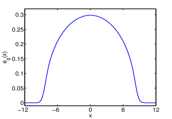
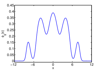
Fig. 1: Ground states $\phi_{g}(x)$ for Case I (left) and Case II (right) in §4.1.

4.2 Accuracy test and results in 3D

We take $d=3$ and $\Omega=0$ in (1.7) and (1.6) and consider two different trapping potentials [16]:

Case I. A harmonic oscillator potential (1.5) with $d=3$, $\gamma_{x}=1$, $\gamma_{y}=2$, $\gamma_{z}=4$ and $\beta=200$.

Case II. A harmonic oscillator potential and a potential of a stirrer corresponding to a far-blue detuned Gaussian laser beam

$$V(x,y,z)=\frac{1}{2}(x^{2}+\gamma_{y}^{2}y^{2}+\gamma_{z}^{2}z^{2})+\omega_{0}e^{-\delta((x-r_{0})^{2}+y^{2})}$$

with $\gamma_{y}=1$, $\gamma_{z}=2$, $\omega_{0}=4$, $\delta=1$, $r_{0}=1$ and $\beta=200$.

Table 3: Accuracy of the FD and SP discretizations for Case I in §4.2.

Mesh size	$h=2$	$h=1$	$h=1/2$	$h=1/4$
$\max|\phi_{g}-\phi_{g,h}^{\rm FD}|$	2.28E-02	5.16E-03	1.11E-03	2.51E-04
$|E_{g}-E(\phi_{g,h}^{\rm FD})|$	1.26E-01	5.82E-02	1.44E-02	3.41E-03
$|\mu_{g}-\mu(\phi_{g,h}^{\rm FD})|$	4.45E-02	3.10E-02	9.40E-03	2.23E-03
$\max|\phi_{g}-\phi_{g,h}^{\rm SP}|$	1.10E-02	1.68E-03	8.68E-06	7.34E-10
$|E_{g}-E(\phi_{g,h}^{\rm SP})|$	1.01E-01	6.49E-05	1.45E-08	1.09E-11
$|\mu_{g}-\mu(\phi_{g,h}^{\rm SP})|$	1.57E-01	4.17E-03	5.48E-07	1.55E-11

Again, the ground state is numerically computed by the Algorithm 1 on bounded computational domains $U=(-8,8)\times(-6,6)\times(-4,4)$ and $U=(-8,8)^{3}$ for Case I and II, respectively, which are partitioned uniformly with the same number of nodes in each direction. Let $h$ be the mesh size in the $x$-direction. Again, we set $\epsilon_{0}=10^{-12}$ in (4.1). Let $\phi_{g,h}^{\rm FD}$ and $\phi_{g,h}^{\rm SP}$ be the numerical ground states obtained with the mesh size $h$ by using FD and SP discretization, respectively. Table 3 depicts the numerical errors for Case I, and respectively, Table 4 for Case II.

Table 4: Accuracy of the FD and SP discretizations for Case II in §4.2.

Mesh size	$h=2$	$h=1$	$h=1/2$	$h=1/4$
$\max|\phi_{g}-\phi_{g,h}^{\rm FD}|$	1.61E-02	7.92E-03	1.69E-03	3.92E-04
$|E_{g}-E(\phi_{g,h}^{\rm FD})|$	6.76E-01	6.06E-02	1.33E-02	3.16E-03
$|\mu_{g}-\mu(\phi_{g,h}^{\rm FD})|$	5.37E-01	6.16E-02	8.09E-03	1.92E-03
$\max|\phi_{g}-\phi_{g,h}^{\rm SP}|$	1.69E-01	2.57E-03	4.38E-05	1.18E-08
$|E_{g}-E(\phi_{g,h}^{\rm SP})|$	1.87E-01	6.69E-03	9.55E-06	6.34E-12
$|\mu_{g}-\mu(\phi_{g,h}^{\rm SP})|$	5.69E-01	2.21E-02	7.79E-06	9.85E-11

Again, from Tables 3 and 4, it is observed that the SP discretization is spectrally accurate, while the FD discretization has only second order accuracy for computing the ground state of BEC in 3D. Hence, when high accuracy is required and/or the solution has multiscale phenomena, the SP discretization is preferred since it needs much fewer grid points, and thus it saves significantly memory cost and computational cost.

Again, for comparison with existing numerical results in the literatures [7, 10, 14, 16, 17], Figure 2 plots the ground states $\phi_{g}(x,0,z)$ obtained by the SP discretization for cases I and II. In addition, their energy, chemical potential and root mean squares are obtained as for Case I: $E_{g}=8.3345$, $\mu_{g}=11.0102$, $x_{\mathrm{rms}}=1.6710$, $y_{\mathrm{rms}}=0.8751$, and $z_{\mathrm{rms}}=0.4884$; and for Case II: $E_{g}=5.2696$, $\mu_{g}=6.7019$, $x_{\mathrm{rms}}=1.3744$, $y_{\mathrm{rms}}=1.4358$ and $z_{\mathrm{rms}}=0.7043$. These numerical results agree very well with those reported in the literatures [7, 10, 14, 16, 17].

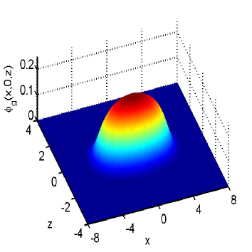
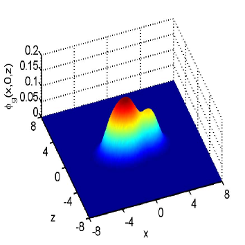
Fig. 2: Ground states $\phi_{g}(x,0,z)$ for Case I (left) and Case II (right) in §4.2.

To demonstrate the high resolution of the SP discretization and compare our algorithm with existing numerical methods [7, 10, 14], we also apply our algorithm to compute the ground state of BEC in 3D with a combined harmonic and optical lattice potential [14] as

(4.5) $$V(x,y,z)=\frac{1}{2}\left(x^{2}+y^{2}+z^{2}\right)+50\left[\sin^{2}\left(\frac{\pi x}{4}\right)+\sin^{2}\left(\frac{\pi y}{4}\right)+\sin^{2}\left(\frac{\pi z}{4}\right)\right],$$

together with different interaction constants $\beta=100$, $800$ and $6400$. The ground state is numerically computed by the Algorithm 1 on bounded computational domains $U=(-8,8)^{3}$ for $\beta=100$ and $800$, and $U=(-12,12)^{3}$ for $\beta=6400$, which are partitioned uniformly with the number of nodes $N_{1}=N_{2}=N_{3}=2^{7}+1$ in each direction. The stopping criterion is set to the default value.

Table 5: Comparison of numerical results computed by Algorithm 1 (top half part with rows 2–4) and BESP implemented in GPELab (bottom half part with rows 5–7) for trapping potential (4.5) with different $\beta$.

$\beta$	$\max|\phi_{g}|^{2}$	$E(\phi_{g})$	$\mu_{g}$	$x_{\mathrm{rms}}$	$y_{\mathrm{rms}}$	$z_{\mathrm{rms}}$	iter	nfe	cpu (s)
100	0.2536	23.2356	27.4757	1.8716	1.8716	1.8716	112	115	76.47
800	0.0490	33.8023	40.4476	2.6620	2.6620	2.6620	260	279	183.34
6400	0.0098	52.4955	63.7146	3.3685	3.3685	3.3685	305	327	217.03
100	0.2536	23.2356	27.4757	1.8717	1.8717	1.8717	188	-	914.53
800	0.0490	33.8023	40.4476	2.6620	2.6620	2.6620	494	-	2513.75
6400	0.0098	52.4955	63.7149	3.3684	3.3684	3.3684	747	-	4014.17

Table 5 depicts the maximum value of the wave function $\max|{\phi_{g}}|^{2}$, the energy $E(\phi_{g})$, the chemical potential $\mu_{g}$ and the root mean squares $x_{\rm rms}$, $y_{\rm rms}$ and $z_{\rm rms}$ for different interaction constants $\beta$, as well as the number of iterations (iter), the number of function evaluations (nfe) and the computational time (cpu). For comparison, we also display numerical results obtained by using the BESP method implemented in GPELab [7] (a MATLAB toolbox designed for computing ground state and dynamics of BEC) with time step taken as $\Delta t=10^{-2}$ and all other setting the same as above. In addition, Figure 3 shows the isosurface plots and their corresponding slice views of the ground states for different $\beta$.

Fig. 3: Isosurfaces (left column) and their corresponding slice views (right column) of the ground states $\phi_{g}(x,y,z)$ of a BEC in 3D with combined harmonic and optical lattice potential (4.5) for different $\beta=100,\,800,\,6400$ (from top to bottom).

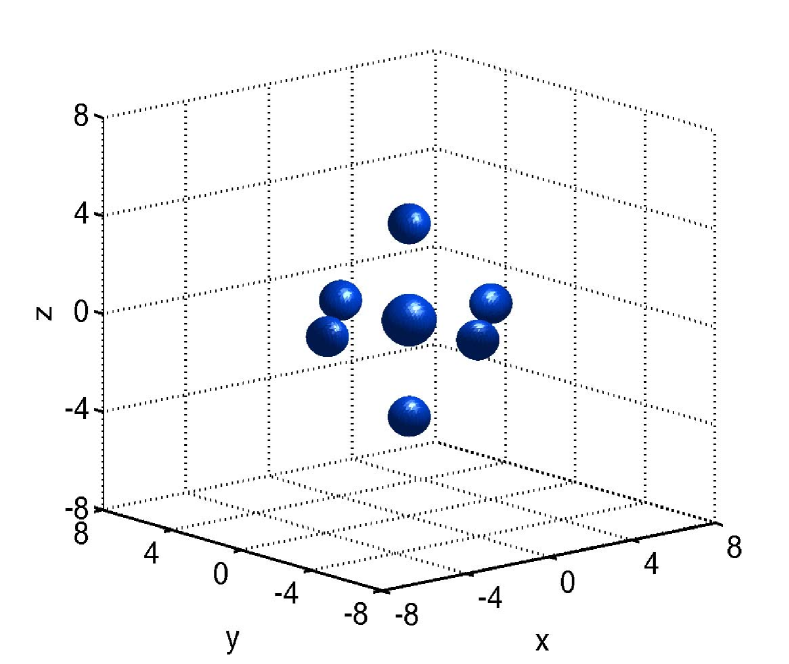
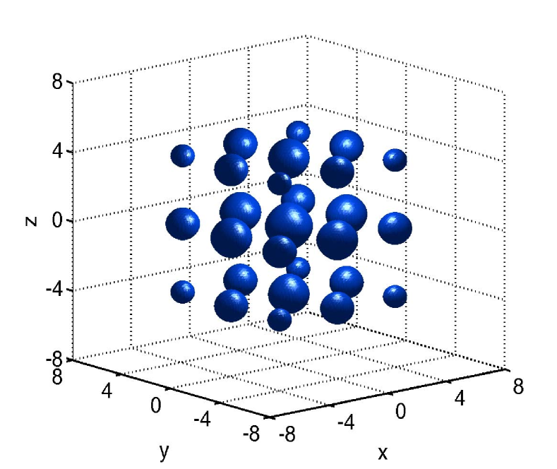
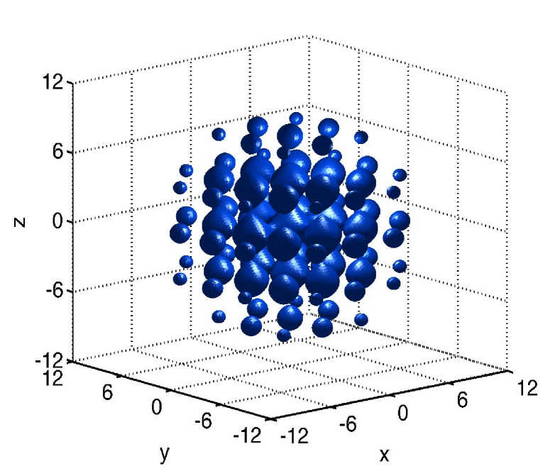
(a) Isosurface plot

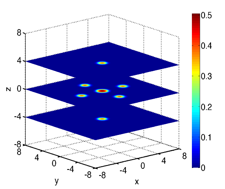
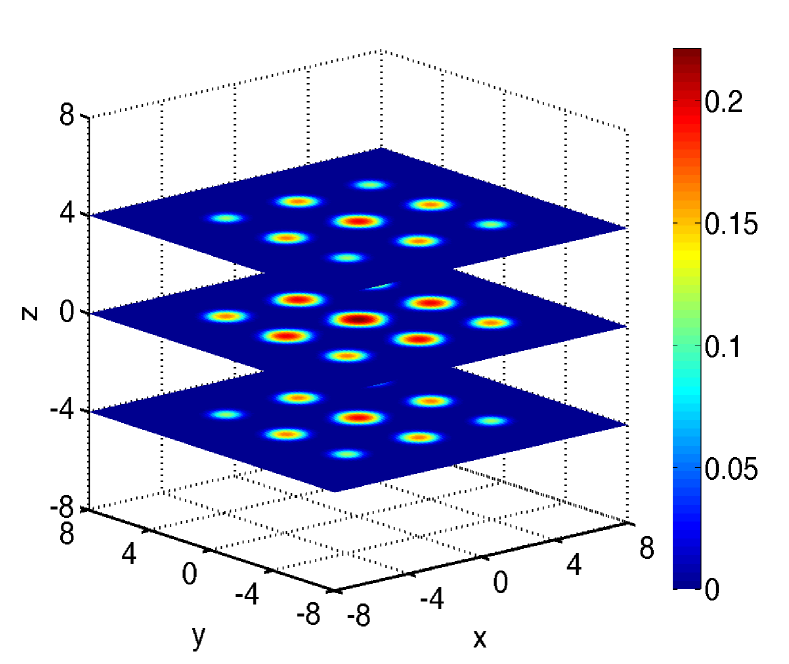
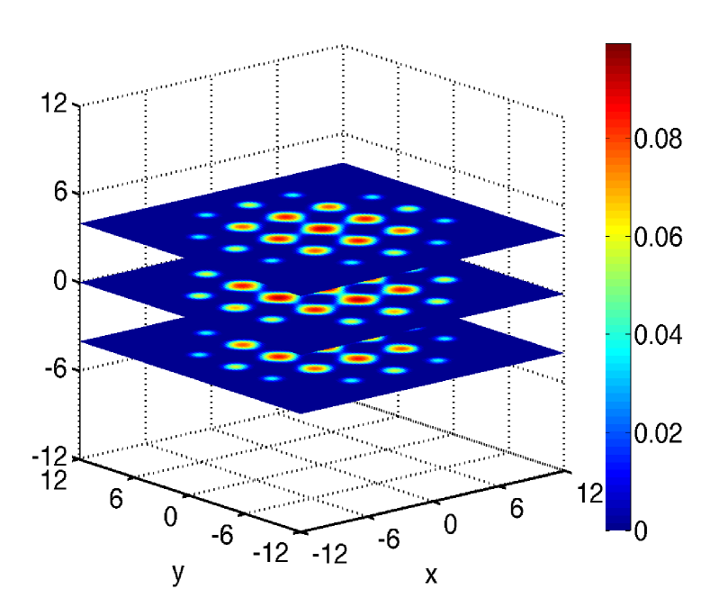
(b) Slice plot

From Table 5, we can see that the Algorithm 1 converges to the ground state much faster than the BESP method presented in [10, 14] for all $\beta$ in computing the ground state of BEC in 3D.

4.3 Results for rotating BEC in 2D

We take $d=2$ and the harmonic potential (1.5) with $\gamma_{x}=\gamma_{y}=1$ in (1.7) and (1.6) and consider different $\beta$ and $\Omega$. The ground state is numerically computed by the regularized Newton method (i.e. Algorithm 2) with the FP discretization on bounded computational domains $U=(-10,10)^{2}$ and $U=(-12,12)^{2}$ for $\beta=500$ and $\beta=1000$, respectively. The domains are partitioned uniformly with the number of nodes $N_{1}=N_{2}=2^{8}+1$ in each direction. In our computations, in the Algorithm 2, we first call the gradient type method, i.e., Algorithm 1, with a maximum number of iterations $K_{\rm init}=100$ to obtain a good initial guess $X^{(1)}$. Then the regularized Newton subproblem is solved by the Algorithm 1 up to a maximum number of iterations $K_{\rm sub}=200$. In order to reduce the computational cost, the cascadic multigrid method (i.e., Algorithm 3) is applied for mesh refinement with the coarsest mesh $\mathcal{T}^{0}$ chosen with the number of nodes $N_{1}=N_{2}=2^{4}+1$ in each direction.

For a rotating BEC, the ground state is a complex-valued function, and thus it is very tricky to choose a proper initial data such that the numerical result is guaranteed to be the ground state. Similarly to those in the literatures [19], here we test our algorithms with the following different initial solutions

$${\rm(a)}\ \phi_{a}(x,y)=\frac{1}{\sqrt{\pi}}e^{-(x^{2}+y^{2})/2},$$

$${\rm(b)}\ \phi_{b}(x,y)=\frac{x+iy}{\sqrt{\pi}}e^{-(x^{2}+y^{2})/2},\qquad(\bar{b})\ \phi_{\bar{b}}(x,y)=\bar{\phi}_{b}(x,y),$$

$${\rm(c)}\ \phi_{c}(x,y)=\frac{[\phi_{a}(x,y))+\phi_{b}(x,y)]/2}{\|[\phi_{a}(x,y))+\phi_{b}(x,y)]/2\|},\qquad(\bar{c})\ \phi_{\bar{c}}(x,y)=\bar{\phi}_{c}(x,y),$$

$${\rm(d)}\ \phi_{d}(x,y)=\frac{(1-\Omega)\phi_{a}(x,y))+\Omega\phi_{b}(x,y)}{\|(1-\Omega)\phi_{a}(x,y))+\Omega\phi_{b}(x,y)\|},\qquad(\bar{d})\ \phi_{\bar{b}}(x,y)=\bar{\phi}_{d}(x,y).$$

Table 6 displays the energy obtained numerically with different initial data selected in the above with $\beta=500$ for different $\Omega=0.00$, $0.25$, $0.50$, $0.60$, $0.70$, $0.80$, $0.90$ and $0.95$ (in the table, we use a “$\dagger$” sign to indicate the one with the lowest energy among different initial data for given $\beta$ and $\Omega$), and Table 7 summarizes the lowest energy among different initial data and the corresponding number of iterations and computation time for $\beta=500$ with different $\Omega$. Figure 4 plots the ground state density $|\phi_{g}(x,y)|^{2}$ for $\beta=500$ with different $\Omega$. In addition, Tables 8-9 and Figure 5 present similar numerical results for $\beta=1000$.

Table 6: Energy obtained numerically with different initial data of rotating BECs for $\beta=500$ and different $\Omega$ in §4.3.

$\Omega$	0.00	0.25	0.50	0.60	0.70	0.80	0.90	0.95
$({\rm a})$	8.5118	8.5118	8.0246	7.5890	6.9731	6.1016	4.7778	3.7417
$({\rm b})$	8.5118	8.5106	8.0246	7.5845	6.9731	6.1055	4.7778	3.7417
$({\rm\bar{b}})$	8.5118	8.5118	8.0197†	7.5890	6.9731	6.1016	4.7778	3.7416
$({\rm c})$	8.5118	8.5106	8.0246	7.5890	6.9726	6.1016	4.7778	3.7417
$({\rm\bar{c}})$	8.5118	8.5118	8.0246	7.5890	6.9731	6.0997	4.7778	3.7415
$({\rm d})$	8.5118†	8.5106†	8.0246	7.5890	6.9726†	6.0997†	4.7778†	3.7415†
$({\rm\bar{d}})$	8.5118	8.5118	8.0246	7.5845†	6.9731	6.1016	4.7778	3.7416

Table 7: Ground state energy, the number of iterations for the regularized Newton method (iter) on the finest mesh and the total computational time (cpu) of rotating BECs for $\beta=500$ and different $\Omega$ in §4.3.

$\Omega$	0.00	0.25	0.50	0.60	0.70	0.80	0.90	0.95
iter	3	3	3	128	49	18	69	4
cpu (s)	1.14	18.71	41.57	355.63	147.03	130.87	286.12	56.08
Energy	8.5118	8.5106	8.0197	7.5845	6.9726	6.0997	4.7778	3.7415

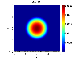
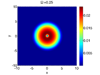
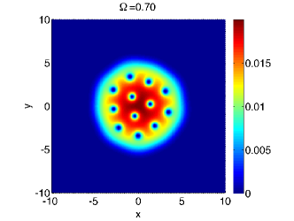
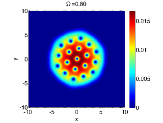
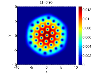
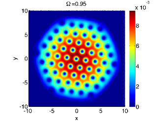
Fig. 4: Plots of the ground state density $|\phi_{g}(x,y)|^{2}$ – corresponding to the energy listed in the Table 6 – of rotating BECs for $\beta=500$ and different $\Omega$ in §4.3.

Table 8: Energy obtained numerically with different initial data of rotating BECs for $\beta=1000$ and different $\Omega$ in §4.3.

$\Omega$	0.00	0.25	0.50	0.60	0.70	0.80	0.90	0.95
$({\rm a})$	11.9718	11.9718	11.0954†	10.4392	9.5335	8.2610	6.3608	4.8830
$({\rm b})$	11.9718	11.9266	11.1326	10.4392	9.5283	8.2610	6.3607	4.8825
$({\rm\bar{b}})$	11.9718	11.9266	11.1054	10.4392	9.5335	8.2631	6.3607	4.8827
$({\rm c})$	11.9718	11.9165	11.1054	10.4392	9.5289	8.2610	6.3607	4.8823†
$({\rm\bar{c}})$	11.9718	11.9165	11.1326	10.4392	9.5283	8.2610	6.3607	4.8825
$({\rm d})$	11.9718	11.9266	11.1054	10.4392	9.5289	8.2632	6.3608	4.8825
$({\rm\bar{d}})$	11.9718†	11.9165†	11.1326	10.4392†	9.5283†	8.2610†	6.3607†	4.8830

Table 9: Ground state energy, the number of iterations for the regularized Newton method (iter) on the finest mesh and the total computational time (cpu) of rotating BECs for $\beta=1000$ and different $\Omega$ in §4.3.

$\Omega$	0.00	0.25	0.50	0.60	0.70	0.80	0.90	0.95
iter	3	3	3	10	10	72	41	157
cpu (s)	1.18	28.52	108.98	106.86	105.28	313.67	825.12	751.72
Energy	11.9718	11.9165	11.0954	10.4392	9.5283	8.2610	6.3607	4.8823

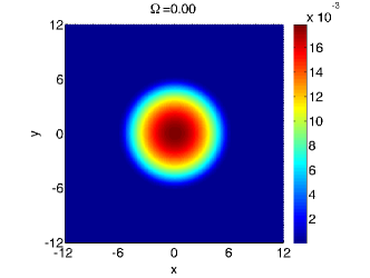
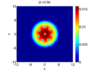
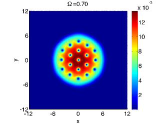
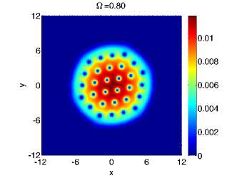
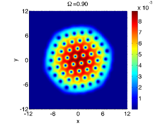
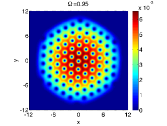
Fig. 5: Plots of the ground state density $|\phi_{g}(x,y)|^{2}$ – corresponding to the energy listed in the Table 8 – of rotating BECs for $\beta=1000$ and different $\Omega$ in §4.3.

From Tables 6-9, among those different initial data, either (d) or ($\bar{\rm d}$) gives the lowest energy in most cases. Thus, in practical computations, we recommend to choose either (d) or ($\bar{\rm d}$) as the initial data. Also, it is observed that the regularized Newton algorithm converges quickly to the stationary solution within very few iterations, even for strong interaction, i.e., $\beta\gg 1$, and fast rotation i.e., $\Omega$ is near $1$. Compared with the normalized gradient flow method via BEFD or BESP discretization for computing ground state of a rotating BEC [3, 4, 7, 10, 19], the regularized Newton algorithm significantly reduces the computational time.

4.4 Application to compute asymmetric excited states

When the trapping potential $V(\mathbf{x})$ in (1.7) is symmetric and the BEC is non-rotating, similarly to those numerical methods presented in the literatures [10, 14, 16, 17], our numerical methods can also be applied to compute the asymmetric excited states provided that the initial data is chosen as an asymmetric function. To demonstrate this, we take $d=2$, $\Omega=0$ and $\beta=500$ in (1.7) and the trapping potential is chosen as a combined harmonic and optical lattice potential

(4.6) $$V(x,y)=\frac{1}{2}\left(x^{2}+y^{2}\right)+50\left[\sin^{2}\left(\frac{\pi x}{4}\right)+\sin^{2}\left(\frac{\pi y}{4}\right)\right].$$

The ground and asymmetric states are numerically computed by the Algorithm 1 via the SP discretization on the bounded computational domain $U=(-16,16)^{2}$ which is partitioned uniformly with the number of nodes $N_{1}=N_{2}=2^{8}+1$ in each direction. The initial data is chosen as the TF approximation (4.2) for computing the ground state $\phi_{g}$, as $\phi_{0}(x,y)=\frac{\sqrt{2}x}{\pi^{1/2}}e^{-(x^{2}+y^{2})/2}$ for the asymmetric excited state in the $x$-direction $\phi_{10}$, as $\phi_{0}(x,y)=\frac{\sqrt{2}y}{\pi^{1/2}}e^{-(x^{2}+y^{2})/2}$ for the asymmetric excited state in the $y$-direction $\phi_{01}$, and as $\phi_{0}(x,y)=\frac{2xy}{\pi^{1/2}}e^{-(x^{2}+y^{2})/2}$ for the asymmetric excited state in both $x$- and $y$-directions $\phi_{11}$, respectively. The stopping criterion is set to the default value. Table 10 lists different quantities of these states and computational cost by our algorithm. In addition, Figure 6 shows contour plots of these states.

Table 10: Different quantities of the ground and asymmetric excited states and the corresponding computational cost for a BEC in 2D with the potential (4.6) and $\beta=500$ in §4.4.

$\phi$	$\max|\phi|^{2}$	$E(\phi)$	$\mu(\phi)$	$x_{\mathrm{rms}}$	$y_{\mathrm{rms}}$	iter	nfe	cpu (s)
$\phi_{g}$	0.0820	32.2079	41.7854	2.9851	2.9851	365	380	3.99
$\phi_{10}$	0.0746	34.6053	43.8248	3.3029	2.8741	285	301	3.18
$\phi_{01}$	0.3749	34.6053	43.8248	2.8741	3.3029	272	288	3.03
$\phi_{11}$	0.0666	37.0864	46.1442	3.1434	3.1434	117	125	1.32

Fig. 6: Contour plots of the ground state $\phi_{g}$ (a), asymmetric excited state in the $x$-direction $\phi_{10}$ (b), (c) asymmetric excited state in the $y$-direction $\phi_{01}$ (c), and asymmetric excited state in both $x$- and $y$- directions $\phi_{11}$ (d) of a BEC in 2D with the potential (4.6) and $\beta=500$ in §4.4.

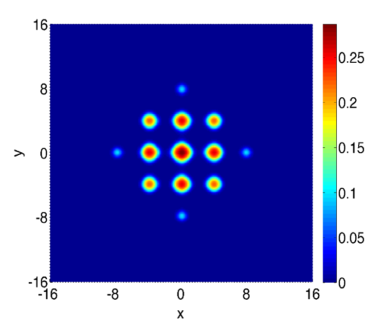
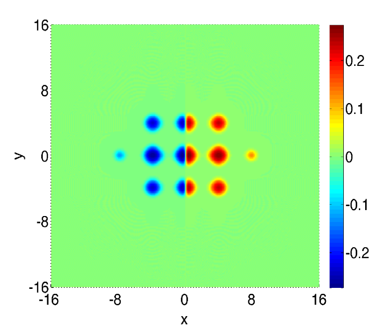
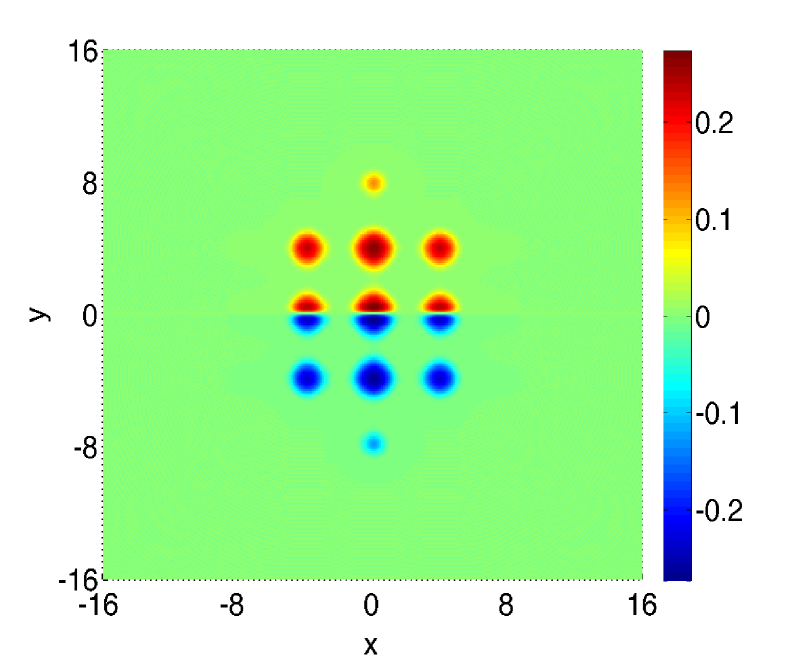
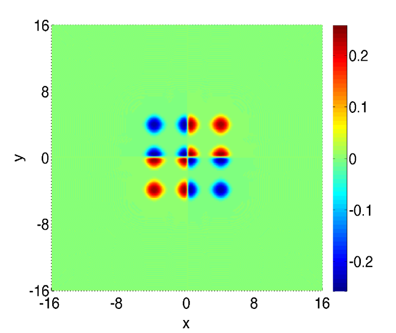
From Table 10 and Figure 6, we can see that our algorithm can be used to compute the asymmetric excited states provided that the initial data is taken as asymmetric functions. The numerical results from our algorithm agree very well with those reported in the literatures [10, 14, 16, 17]. However, our algorithm is much faster than those methods in the literatures [10, 14, 16, 17] for computing the asymmetric excited states.

5 Concluding remarks

Different spatial discretizations including the finite difference method, sine pesudospectral and Fourier pseudospectral methods were adopted to discretize the energy functional and constraint for computing the ground state of Bose-Einstein condensation (BEC). Then the original infinitely dimensional constrained minimization problem was reduced to a finite dimensional minimization problem with a spherical constraint. A regularized Newton method was proposed by using a feasible gradient type method as an initial approximation and solving a standard trust-region subproblem obtained from approximating the energy functional by its second-order Taylor expansion with a regularized term at each Newton iteration as well as adopting a cascadic multigrid technique for selecting initial data. The convergence of the method was established by the standard optimization theory. Extensive numerical examples of non-rotating BEC in 1D and 3D and rotating BEC in 2D with different trapping potentials and parameter regimes demonstrated the efficiency and accuracy as well as robustness of our method. Comparison to existing numerical methods in the literatures showed that our numerical method is significantly faster than those methods proposed in the literatures for computing ground states of BEC.

References

- [1] P.-A. Absil, R. Mahony, and R. Sepulchre, Optimization Algorithms on Matrix Manifolds, Princeton University Press, Princeton, NJ, 2008.
- [2] S.K. Adhikari, Numerical solution of the two-dimensional Gross-Pitaevskii equation for trapped interacting atoms, Phys. Lett. A, 265 (2000), pp. 91–96.
- [3] A. Aftalion and Q. Du, Vortices in a rotating Bose-Einstein condensate: Critical angular velocities and energy diagrams in the Thomas-Fermi regime, Phys. Rev. A, 64 (2001), article 063603.
- [4] A. Aftalion and I. Danaila, Three-dimensional vortex configurations in a rotating Bose Einstein condensate, Phys. Rev. A, 68 (2003), article 023603.
- [5] M.H. Anderson, J.R. Ensher, M.R. Mattews, C.E. Wieman, and E.A. Cornell, Observation of Bose-Einstein condensation in a dilute atomic vapor, Science, 269 (1995), pp. 198–201.
- [6] J.R. Anglin and W. Ketterle, Bose-Einstein condensation of atomic gases, Nature, 416 (2002), pp. 211–218.
- [7] X. Antoine and R. Duboscq, GPELab, a Matlab toolbox to solve Gross-Pitaevskii equations I: Computation of stationary solutions, Comput. Phys. Comm., 185 (2014), pp. 2969–2991.
- [8] X. Antoine and R. Duboscq, Robust and Efficient Preconditioned Krylov Spectral Solvers for Computing the Ground States of Fast Rotating and Strongly Interacting Bose-Einstein Condensates, J. Comput. Phys., 258 (2014), pp. 509-523.
- [9] W. Bao, Ground states and dynamics of multi-component Bose-Einstein condensates, Multiscale Model. Simul., 2 (2004), pp. 210–236.
- [10] W. Bao and Y. Cai, Mathematical theory and numerical methods for Bose-Einstein condensation, Kinet. Relat. Mod., 6 (2013), pp. 1–135.
- [11] , Ground states of two-component Bose-Einstein condensates with an internal atomic Josephson junction, East Asia J. Appl. Math., 1 (2011), pp. 49-81.
- [12] , Ground states and dynamics of spin-orbit-coupled Bose-Einstein condensates, SIAM J. Appl. Math., 75 (2015), pp. 492-517.
- [13] W. Bao, Y. Cai and H. Wang, Efficient numerical methods for computing ground states and dynamics of dipolar Bose-Einstein condensates, J. Comput. Phys., 229 (2010), pp. 7874-7892.
- [14] W. Bao, I.L. Chern, and F.Y. Lim, Efficient and spectrally accurate numerical methods for computing ground and first excited states in Bose-Einstein condensates, J. Comput. Phys., 219 (2006), pp. 836–854.
- [15] W. Bao, I.L. Chern, and Y. Zhang, Efficient numerical methods for computing ground states of spin-1 Bose-Einstein condensates based on their characterizations, J. Comput. Phys., 253 (2013), pp. 189–208.
- [16] W. Bao and Q. Du, Computing the ground state solution of Bose-Einstein condensates by a normalized gradient flow, SIAM J. Sci. Comput., 25 (2004), pp. 1674–1697.
- [17] W. Bao and W. Tang, Ground state solution of Bose-Einstein condensate by directly minimizing the energy functional, J. Comput. Phys., 187 (2003), pp. 230–254.
- [18] W. Bao and H. Wang, A mass and magnetization conservative and energy-diminishing numerical method for computing ground state of spin-1 Bose-Einstein condensates, SIAM J. Numer. Anal., 45 (2007), pp. 2177–2200.
- [19] W. Bao, H. Wang, and P.A. Markowich, Ground, symmetric and central vortex states in rotating Bose-Einstein condensates, Comm. Math. Sci., 3 (2005), pp. 57–88.
- [20] J. Barzilai and J.M. Borwein, Two-point step size gradient methods, IMA J. Numer. Anal., 8 (1988), pp. 141–148.
- [21] F.A. Bornemann and P. Deuflhard, The Cascadic multigrid method for elliptic problems, Numer. Math., 75 (1996), pp. 135-152.
- [22] C.C. Bradley, C.A. Sackett, J.J. Tollett, and R.G. Hulet, Evidence of Bose-Einstein condensation in an atomic gas with attractive interations, Phys. Rev. Lett., 75 (1995), pp. 1687–1690.
- [23] E. Cancès, R. Chakir and Y. Maday, Numerical analysis of nonlinear eigenvalue problems, J. Sci. Comput., 45 (2010), pp. 90-117.
- [24] M.M. Cerimele, M.L. Chiofalo, F. Pistella, S. Succi, and M.P. Tosi, Numerical solution of the Gross-Pitaevskii equation using an explicit finite-difference scheme: An application to trapped Bose-Einstein condensates, Phys. Rev. E, 62 (2009), pp. 1382–1389.
- [25] S.-L. Chang, C.-S. Chien and B.-W. Jeng, Computing wave functions of nonlinear Schrödinger equations: A time-independent approach, J. Comput. Phys., 226 (2007), pp. 104-130.
- [26] S.M. Chang, W.W. Lin, and S.F. Shieh, Gauss-Seidel-type methods for energy states of a multi-component Bose-Einstein condensate, J. Comput. Phys., 202 (2005), pp. 367–390.
- [27] M.L. Chiofalo, S. Succi, and M.P. Tosi, Ground state of trapped interacting Bose-Einstein condensates by an explicit imaginary-time algorithm, Phys. Rev. E, 62 (2000), pp. 7438–7444.
- [28] A.R. Conn, N.I.M. Gould, and P.L. Toint, Trust-Region Methods, MPS/SIAM Series on Optimization, Society for Industrial and Applied Mathematics, Philadelphia, PA, 2000.
- [29] F. Dalfovo, S. Giorgini, L.P. Pitaevskii, and S. Stringari, Theory of Bose-Einstein condensation in trapped gases, Rev. Mod. Phys., 71 (1999), pp. 463–512.
- [30] I. Danaila and P. Kazemi, A new Sobolev gradient method for direct minimization of the Gross-Pitaevskii energy with rotation, SIAM J. Sci. Comput., 32 (2010), pp. 2447 C2467.
- [31] K.B. Davis, M.O. Mewes, M.R. Andrews, N.J. van Druten, D.S. Durfee, D.M. Kurn, and W. Ketterle, Bose-Einstein condensation in a gas of sodium atoms, Phys. Rev. Lett., 75 (1995), pp. 3969–3973.
- [32] R.J. Dodd, Approximate solutions of the nonlinear Schrödinger equation for ground and excited states of Bose-Einstein condensates, J. Res. Natl. Inst. Stan., 101 (1996), pp. 545–552.
- [33] M. Edwards and K. Burnett, Numerical solution of the nonlinear Schrödinger equation for small samples of trapped neutral atoms, Phys. Rev. A, 51 (1995), pp. 1382–1386.
- [34] A.L. Fetter, Rotating trapped Bose-Einstein condensates, Rev. Mod. Phys., 81 (2009), pp. 647–691.
- [35] J.J. Garcia-Ripoll and V.M. Perez-Garcia, Optimizing Schrödinger functional using Sobolev gradients: applications to quantum mechanics and nonlinear optics, SIAM J. Sci. Comput., 23 (2001), pp. 1315-1333.
- [36] E.P. Gross, Structure of a quantized vortex in boson systems, Nuovo. Cimento., 20 (1961), pp. 454–477.
- [37] B. Jiang and Y. Dai, A framework of constraint preserving update schemes for optimization on Stiefel manifold, arXiv:1301.0172, (2013).
- [38] A.J. Leggett, Bose-Einstein condensation in the alkali gases: some fundamental concepts, Rev. Mod. Phys., 73 (2001), pp. 307–356.
- [39] E.H. Lieb and R. Seiringer, Derivation of the Gross-Pitaevskii equation for rotating Bose gases, Comm. Math. Phys., 264 (2006), pp. 505–537.
- [40] E.H. Lieb, R. Seiringer and J. Yngvason, Bosons in a trap: A rigorous derivation of the Gross-Pitaevskii energy functional, Phys. Rev. A, 61 (2000), article 043602.
- [41] M.R. Matthews, B.P. Anderson, P.C. Haljan, D.S. Hall, C.E. Wieman, and E.A. Cornell, Vortices in a Bose-Einstein condensate, Phys. Rev. Lett., 83 (1999), pp. 2498–2501.
- [42] J. Nocedal and S.J. Wright, Numerical Optimization, Springer Series in Operations Research and Financial Engineering, Springer, New York, second ed., 2006.
- [43] C.J. Pethick and H. Smith, Bose-Einstein Condensation in Dilute Gases, Cambridge University Press, (2002).
- [44] L.P. Pitaevskii, Vortex lines in an imperfect Bose gas, Soviet Phys. JETP, 13 (1961), pp. 451–454.
- [45] L.P. Pitaevskii and S. Stringari, Bose-Einstein Condensation, Calrendon Press, Oxford, (2003).
- [46] C. Raman, J.R. Abo-Shaeer, J.M. Vogels, K. Xu, and W. Ketterle, Vortex nucleation in a stirred Bose-Einstein condensate, Phys. Rev. Lett., 87 (2001), p. 210402.
- [47] P.A. Ruprecht, M.J. Holland, K. Burrett, and M. Edwards, Time-dependent solution of the nonlinear Schrödinger equation for Bose-condensed trapped neutral atoms, Phys. Rev. A, 51 (1995), pp. 4704–4711.
- [48] B.I. Schneider and D.L. Feder, Numerical approach to the ground and excited states of a Bose-Einstein condensated gas confined in a completely anisotropic trap, Phys. Rev. A, 59 (1999), p. 2232.
- [49] W. Sun and Y.-X, Yuan, Optimization Theory and Methods, vol. 1 of Springer Optimization and Its Applications, Springer, New York, 2006.
- [50] Z. Wen, A. Milzarek, M. Ulbrich, and H. Zhang, Adaptive regularized self-consistent field iteration with exact Hessian for electronic structure calculation, SIAM J. Sci. Comput., 35 (2013), pp. A1299–A1324.
- [51] Z. Wen and W. Yin, A feasible method for optimization with orthogonality constraints, Math. Program. Ser. A., 142 (2013), pp. 397–434.
- [52] A.H. Zhou, An analysis of finite-dimensional approximations for the ground state solution of Bose-Einstein condensates, Nonlinearity, 17 (2004), pp. 541–550.