Block-Maxima of Vines

Abstract

We examine the dependence structure of finite block-maxima of multivariate distributions. We provide a closed form expression for the copula density of the vector of the block-maxima. Further, we show how partial derivatives of three-dimensional vine copulas can be obtained by only one-dimensional integration. Combining these results allows the numerical treatment of the block-maxima of any three-dimensional vine copula for finite block-sizes. We look at certain vine copula specifications and examine how the density of the block-maxima behaves for different block-sizes. Additionally, a real data example from hydrology is considered. In extreme-value theory for multivariate normal distributions, a certain scaling of each variable and the correlation matrix is necessary to obtain a non-trivial limiting distribution when the block-size goes to infinity. This scaling is applied to different three-dimensional vine copula specifications.

Keywords: Multivariate copula, vine copulas, finite block-maxima, scaled block-maxima, extreme-value scaling.

1 Copula Density of the Distribution of Block-Maxima

Basically, block-maxima have been used in extreme-value theory as one approach to derive the family of General Extreme-Value (GEV) distributions (McNeil et al. (2010)). In the recent past the block-maxima method has been studied more thoroughly and compared to the peaks-over-threshold (POT) method in Ferreira et al. (2014) and Jarušková and Hanek (2006). Dombry (2013) justifies the usage of a maximum-likelihood estimator for the extreme-value index within the block-maxima framework. The numerical convergence of the block-maxima approach to the GEV distribution is examined in Faranda et al. (2011). Moreover, the block-maxima method has found its way into many application areas: Marty and Blanchet (2012) investigate long-term changes in annual maximum snow depth and snowfall in Switzerland. Temperature, precipitation, wind extremes over Europe are analyzed in Nikulin et al. (2011). A spatial application can be found in Naveau et al. (2009). Rocco (2014) provides an overview over the concepts of extreme-value theory being used in finance. While many of the articles use univariate concepts, Bücher and Segers (2013) treats how to estimate extreme-value copulas based on block-maxima of a multivariate stationary time series. In contrast to the existing literature (known to the authors), in the following we will consider finite block-maxima of multivariate random variables focusing on the dependence structure.

Let $\mathbf{U}=(U_{1},\ldots,U_{d})^{\prime}$ be a random vector with $\mathcal{U}[0,1]$-distributed margins, copula $C$ and copula density $c$. We consider $n$ i.i.d. copies $\mathbf{U}_{i}=(U_{i,1},\ldots,U_{i,d})^{\prime}$ of $\mathbf{U}$, $i=1,\ldots,n$. We apply the inverse probability integral transform to each component of $\mathbf{U}_{i}$ to obtain marginally normalized data (called z-scale):

$$\mathbf{Z}_{i}=(Z_{i,1},\ldots,Z_{i,d})^{\prime}\text{ with }Z_{i,j}:=\Phi^{-1}(U_{i,j})\sim\mathcal{N}(0,1),$$

for $i=1,\ldots,n$, $j=1,\ldots,d$, where $\Phi^{-1}$ is the quantile function of the standard normal distribution $\mathcal{N}(0,1)$. We consider this normalized scale since later we want to compare this to the limiting approach used to derive the multivariate Hüsler-Reiss extreme-value copula. We are interested in the distribution $F^{(n)}$ of the vector of componentwise block-maxima

$$\mathbf{M}^{(n)}=(M^{(n)}_{1},\ldots,M^{(n)}_{d})^{\prime}\text{ with }M^{(n)}_{j}:=\max_{i=1,\ldots,n}Z_{i,j}$$

for $j=1,\ldots,d$. According to Sklar (1959) the dependency structure is determined by the corresponding copula $C_{\mathbf{M}^{(n)}}$. Since $Z_{i,j}$, $i=1,\ldots,n$, are i.i.d., we know that the marginal distribution functions of $M^{(n)}_{j}$ are given by

$$F^{(n)}_{j}(m_{j})=\mathbb{P}\left(Z_{1,j}\leq m_{j},\ldots,Z_{n,j}\leq m_{j}\right)=\Phi(m_{j})^{n}$$ (1.1)

and hence the corresponding densities are

$$f^{(n)}_{j}(m_{j})=n\Phi(m_{j})^{n-1}\varphi(m_{j})$$ (1.2)

for $m_{j}\in\mathbb{R}$, $j=1,\ldots,d$. Here $\Phi$ and $\varphi$ denote the distribution function and the density of the standard normal distribution, respectively. Thus, the copula $C_{\mathbf{M}^{(n)}}$ is the distribution function of

$$\mathbf{V}=(V_{1},\ldots,V_{d})^{\prime}\text{ with }V_{j}:=\Phi\left(M_{j}^{(n)}\right)^{n}\sim\mathcal{U}[0,1].$$

For $n\in\mathbb{N}$ the copula of the componentwise maxima $C_{\mathbf{M}^{(n)}}$ can be expressed in terms of the underlying copula $C$ as follows

$$C_{\mathbf{M}^{(n)}}(u_{1},\ldots,u_{d})=C\left(u_{1}^{1/n},\ldots,u_{d}^{1/n}\right)^{n},$$ (1.3)

where $u_{j}\in[0,1]$, $j=1,\ldots,d$. Since $C$ is assumed to have a density $c$, Equation 1.3 yields that $C_{\mathbf{M}^{(n)}}$ also has a density, denoted by $c_{\mathbf{M}^{(n)}}$. Using Sklar’s Theorem, Equations 1.1 and 1.3 imply that the joint distribution function of $\mathbf{M}^{(n)}$ is given by

$$F^{(n)}(m_{1},\ldots,m_{d})=C_{\mathbf{M}^{(n)}}\left(F^{(n)}_{1}(m_{1}),\ldots,F^{(n)}_{d}(m_{d})\right)=C\left(\Phi(m_{1}),\ldots,\Phi(m_{d})\right)^{n}.$$

Theorem 1.1.

The density of the copula of the vector of block-maxima satisfies for $u_{j}\in[0,1]$, $j=1\ldots,d$:

$$c_{\mathbf{M}^{(n)}}(u_{1},\ldots,u_{d})=\frac{1}{n^{d}}\left(\prod_{j=1}^{d}u_{j}\right)^{\frac{1}{n}-1}\sum_{j=1}^{d\wedge n}\Bigg{\{}\frac{n!}{(n-j)!}C\left(u_{1}^{1/n},\ldots,u_{d}^{1/n}\right)^{n-j}\Bigg{.}\\ \Bigg{.}\cdot\sum_{\mathcal{P}\in\mathcal{S}_{d,j}}\prod_{M\in\mathcal{P}}\partial_{M}C\left(u_{1}^{1/n},\ldots,u_{d}^{1/n}\right)\Bigg{\}},$$ (1.4)

where $d\wedge n:=\min\left\{d,n\right\}$, $\mathcal{S}_{d,j}:=\left\{\mathcal{P}|\mathcal{P}\textrm{ partition of }\left\{1,\ldots,d\right\}\textrm{ with }\left|\mathcal{P}\right|=j\right\}$ and

$$\partial_{M}C\left(u_{1}^{1/n},\ldots,u_{d}^{1/n}\right):=\frac{\partial^{p}C(v_{1},\ldots,v_{d})}{\partial v_{m_{1}}\cdots\partial v_{m_{p}}}\bigg{|}_{v_{1}=u_{1}^{1/n},\ldots,v_{d}=u_{d}^{1/n}}$$

for $M=\left\{m_{1},\ldots,m_{p}\right\}\subseteq\left\{1,\ldots,d\right\}$.

The proof of Theorem 1.1 as well as all other proofs can be found in the appendix at the end of this chapter (pages Appendix ff.).

For the joint density $f^{(n)}$ of the block-maxima with marginally normalized data (on the z-scale) we also obtain an explicit expression.

Corollary 1.2.

For $m_{j}\in\mathbb{R}$, $j=1,\ldots,d$, we have

$$f^{(n)}(m_{1},\ldots,m_{d})=\left(\prod_{j=1}^{d}\varphi(m_{j})\right)\cdot\sum_{j=1}^{d\wedge n}\Bigg{\{}\frac{n!}{(n-j)!}\cdot C\left(\Phi(m_{1}),\ldots,\Phi(m_{d})\right)^{n-j}\big{.}\\ \big{.}\cdot\sum_{\mathcal{P}\in\mathcal{S}_{d,j}}\prod_{M\in\mathcal{P}}\partial_{M}C\left(\Phi(m_{1}),\ldots,\Phi(m_{d})\right)\Bigg{\}}.$$ (1.5)

Example 1.3.

Let $d=3$, $n\in\mathbb{N}$, i.e. $\mathbf{U}_{i}=(U_{i,1},U_{i,2},U_{i,3})^{\prime}$, $\mathbf{Z}_{i}=(Z_{i,1},Z_{i,2},Z_{i,3})^{\prime}$ and $\mathbf{M}^{(n)}=(M^{(n)}_{1},M^{(n)}_{2},M^{(n)}_{3})^{\prime}$, $i=1,\ldots,n$. If $n\geq 3$ the copula density of the vector of the block-maxima is given by

$$\begin{split}c_{\mathbf{M}^{(n)}}(u_{1},&u_{2},u_{3})=\frac{(u_{1}u_{2}u_{3})^{\frac{1}{n}-1}}{n^{3}}\cdot\Big{\{}nC\left(u_{1}^{1/n},u_{2}^{1/n},u_{3}^{1/n}\right)^{n-1}c\left(u_{1}^{1/n},u_{2}^{1/n},u_{3}^{1/n}\right)\Big{.}\\ &\quad+n(n-1)C\left(u_{1}^{1/n},u_{2}^{1/n},u_{3}^{1/n}\right)^{n-2}\\ &\quad\cdot\Big{[}\partial_{1}C\left(u_{1}^{1/n},u_{2}^{1/n},u_{3}^{1/n}\right)\partial_{23}C\left(u_{1}^{1/n},u_{2}^{1/n},u_{3}^{1/n}\right)\Big{.}\\ &\quad+\partial_{2}C\left(u_{1}^{1/n},u_{2}^{1/n},u_{3}^{1/n}\right)\partial_{13}C\left(u_{1}^{1/n},u_{2}^{1/n},u_{3}^{1/n}\right)\\ &\Big{.}\quad+\partial_{3}C\left(u_{1}^{1/n},u_{2}^{1/n},u_{3}^{1/n}\right)\partial_{12}C\left(u_{1}^{1/n},u_{2}^{1/n},u_{3}^{1/n}\right)\Big{]}\\ &\quad+n(n-1)(n-2)C\left(u_{1}^{1/n},u_{2}^{1/n},u_{3}^{1/n}\right)^{n-3}\partial_{1}C\left(u_{1}^{1/n},u_{2}^{1/n},u_{3}^{1/n}\right)\\ &\quad\Big{.}\cdot\partial_{2}C\left(u_{1}^{1/n},u_{2}^{1/n},u_{3}^{1/n}\right)\partial_{3}C\left(u_{1}^{1/n},u_{2}^{1/n},u_{3}^{1/n}\right)\Big{\}}.\end{split}$$

2 Vine Copulas

While the catalog of bivariate copula families (see for example Joe (1997)) is large this is not the case for multivariate copula families. They were initially dominated by Archimedean and elliptical copulas, however for complex dependency patterns such as asymmetric dependence in the tails these classes are insufficient. The class of vine copulas (Bedford and Cooke (2002), Kurowicka and Cooke (2006), Aas et al. (2009), Kurowicka and Joe (2011)) can accommodate such patterns. See Stöber and Czado (2012) for a tutorial introduction and Czado (2010) and Czado et al. (2013) for recent reviews. Basically vine copulas are constructed using bivariate copulas called pair copulas as building blocks which are combined to form multivariate copulas using conditioning. The pair copulas represent the copula associated with bivariate conditional distributions. The conditioning variables are determined with the help of a sequence of linked trees called the vine structure. Further it is commonly assumed that the conditioning value does not influence the copula and its parameter. See Stöber et al. (2013) for a discussion of this simplifying condition. Further they show that multivariate Clayton copula is the only Archimedean copula which can be represented as a vine copula, while the multivariate t-copula is the only scale elliptical one. For the multivariate Gaussian copula and the t-copula the needed pair copulas are bivariate Gaussian or t-copulas, respectively. The corresponding parameters are given by (partial) correlation parameters.

Vine copulas allow for product expressions of the density. We only consider three-dimensional vine copulas which can be expressed as

$$c(u_{1},u_{2},u_{3})=c_{12}(u_{1},u_{2})c_{23}(u_{2},u_{3})c_{13;2}(C_{1|2}(u_{1}|u_{2}),C_{3|2}(u_{3}|u_{2})).$$ (2.6)

Here $c_{ij;k}$ denotes the bivariate copula density corresponding to bivariate distribution $(U_{i},U_{j})$ given $U_{k}=u_{k}$ and $C_{i|j}(u_{i}|u_{j})$ denotes the conditional distribution function of $U_{i}$ given $U_{j}=u_{j}$, which can be expressed as

$$C_{i|j}(u_{i}|u_{j})=\frac{\partial}{\partial u_{j}}C_{ij}(u_{i},u_{j})$$

Further we write the bivariate copula densities in terms of their copula, i.e. $c_{ij}(u_{i},u_{j})=\frac{\partial^{2}}{\partial u_{i}\partial u_{j}}C_{ij}(u_{i},u_{j}).$ For the pair copulas $C_{12},C_{23},C_{13;2}$ arbitrary bivariate copulas can be utilized. Many bivariate families including rotations are implemented in the R library VineCopula (see Schepsmeier et al. (2014)), which allows for parameter estimation and model selection of vine copulas in arbitrary dimensions.

Now we will consider the three-dimensional case and derive expressions for the partial derivatives needed in Theorem 1.1 for the expression of the copula density for the block-maxima.

Theorem 2.1.

For the vine copula density (2.6) we have:

1. $C(u_{1},u_{2},u_{3})=\int_{0}^{u_{2}}C_{13;2}\left(C_{1|2}(u_{1}|v_{2}),C_{3|2}(u_{3}|v_{2})\right)dv_{2}$,

2. 1. $\partial_{1}C(u_{1},u_{2},u_{3})=\int_{0}^{u_{2}}\partial_{1}C_{13|2}(C_{1|2}(u_{1}|v_{2}),C_{3|2}(u_{3}|v_{2}))c_{12}(u_{1},v_{2})dv_{2}$,

   2. $\partial_{2}C(u_{1},u_{2},u_{3})=C_{13;2}(C_{1|2}(u_{1}|u_{2}),C_{3|2}(u_{3}|u_{2}))$,

   3. $\partial_{3}C(u_{1},u_{2},u_{3})=\int_{0}^{u_{2}}\partial_{3}C_{13|2}(C_{1|2}(u_{1}|v_{2}),C_{3|2}(u_{3}|v_{2}))c_{23}(v_{2},u_{3})dv_{2}$,

3. 1. $\partial_{12}C(u_{1},u_{2},u_{3})=\partial_{1}C_{13;2}(C_{1|2}(u_{1}|u_{2}),C_{3|2}(u_{3}|u_{2}))c_{12}(u_{1},u_{2})$,

   2. $\partial_{13}C(u_{1},u_{2},u_{3})=\int_{0}^{u_{2}}c_{13;2}(C_{1|2}(u_{1}|v_{2}),C_{3|2}(u_{3}|v_{2}))c_{23}(v_{2},u_{3})c_{12}(u_{1},v_{2})dv_{2}$,

   3. $\partial_{23}C(u_{1},u_{2},u_{3})=\partial_{3}C_{13;2}(C_{1|2}(u_{1}|u_{2}),C_{3|2}(u_{3}|u_{2}))c_{23}(u_{2},u_{3})$,

4. $c(u_{1},u_{2},u_{3})=c_{12}(u_{1},u_{2})c_{23}(u_{2},u_{3})c_{13;2}(C_{1|2}(u_{1}|u_{2}),C_{3|2}(u_{3}|u_{2}))$.

Theorem 2.1 shows that the copula density corresponding to the three-dimensional vector of block-maxima based on an arbitrary vine copula is numerically tractable since only one-dimensional integration is needed. In particular this allows a numerical treatment for the block-size $n$ in a finite setting. Additionally we can use the vine decomposition for a three-dimensional Gaussian or t-copula instead of requiring three-dimensional integration to calculate the corresponding density of the block-maxima. Two examples illustrate this way of proceeding.

Example 2.2.

As a first example we take a three-dimensional Clayton-vine, i.e. all three pair-copulas are bivariate Clayton copulas. As parameters we choose $\delta_{12}=6$, $\delta_{23}=7.09$ and $\delta_{13;2}=4.67$ corresponding to Kendall’s $\tau$ values of $\tau_{12}=0.75$ and $\tau_{23}=0.78$, $\tau_{13;2}=0.70$.

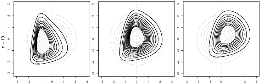
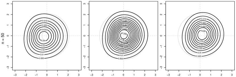
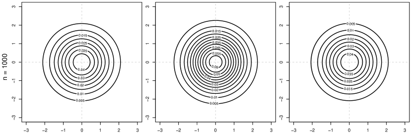
Figure 1: Two-dimensional slices of the copula density for block-maxima of a three-dimensional Clayton-vine with normalized margins ($\tau_{12}=0.75$, $\tau_{23}=0.78$, $\tau_{13;2}=0.7$).

Figure 1 shows the copula density of the block-maxima of this vine with normalized margins (i.e. on the z-level) for block-sizes $n=10,50,10^{3}$. Each row represents one block-size and contains three contour plots. Since it is difficult to plot three-dimensional objects in a simple way we decided not to show the isosurfaces but cut the three-dimensional object into three slices parallel to the z₁-z₂-plane. Each column presents the contourplot of one slice, where the z₃-value is fixed to $\Phi^{-1}(0.2)$, $\Phi^{-1}(0.5)$ or $\Phi^{-1}(0.8)$, respectively. Furthermore, we plotted the contours of the independence copula with normalized margins. One can see that already for $n=10^{3}$ the contours of the copula density of the block-maxima with normalized margins practically coincide with the ones of the independence copula.

Remark 2.3.

Even though it is not known whether all Clayton-vines lie in the domain of attraction of the independence copula, one can show that the Clayton-copula, which can be represented as a Clayton-vine with specific parameter restrictions (Stöber et al. (2013)), lies in the domain of attraction of the independence copula. According to Gudendorf and Segers (2010) an Archimedean copula with generator $\varphi$ lies in the domain of attraction of the Gumbel-copula with parameter $\theta:=-\lim_{s\downarrow 0}\frac{s\varphi^{\prime}(1-s)}{\varphi(1-s)}\in[1,\infty)$ if the limit exists. For the Clayton-copula this limit is equal to 1. Therefore, the copula of the block-maxima of a Clayton-copula converges to the Gumbel-copula with $\theta=1$, which is the independence copula.

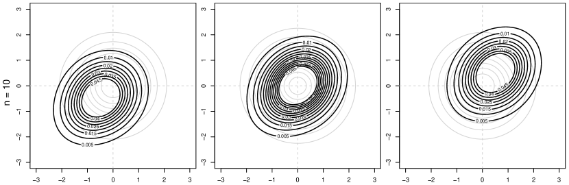
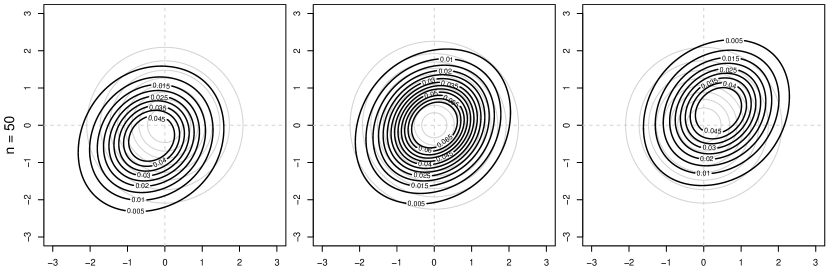
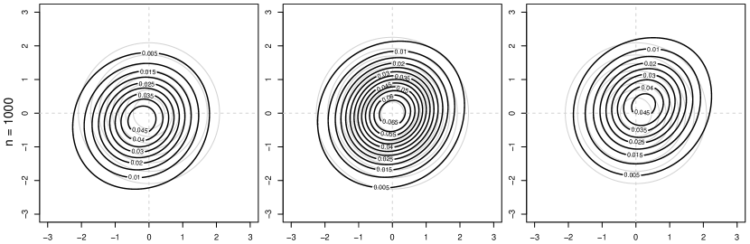
Figure 2: Two-dimensional slices of the copula density for block-maxima of a three-dimensional Gaussian vine with normalized margins ($\tau_{12}=0.5$, $\tau_{23}=0.57$, $\tau_{13;2}=0.35$).

Example 2.4.

The second example we present is a three-dimensional Gaussian vine, i.e. all three pair-copulas are bivariate Gaussian copulas. As parameters we choose $\rho_{12}=0.71$, $\rho_{23}=0.78$ and $\rho_{13;2}=0.52$ corresponding to Kendall’s $\tau$ values of $\tau_{12}=0.50$ and $\tau_{23}=0.57$, $\tau_{13;2}=0.35$.

Figure 2 shows the copula density of the block-maxima of this vine with normalized margins (i.e. on the z-level) for block-sizes $n=10,50,10^{3}$. As above each row represents one block-size and contains three contour plots corresponding to z₃-values fixed to $\Phi^{-1}(0.2)$, $\Phi^{-1}(0.5)$ or $\Phi^{-1}(0.8)$, respectively. Again we detect convergence to the independence copula. This is also what one would expect: Hüsler and Reiss (1989) showed that in order to achieve that the distribution of the maxima of a multivariate Gaussian distribution converges to a non-trivial limiting distribution, a proper scaling of the margins and the correlation coefficients is necessary. This will be discussed in Section 3.

Example 2.5.

Hydrology is one of the areas where block-maxima are important. Especially, the water levels of rivers can be interesting when it comes to analyzing the risk of floods. We consider a three-dimensional data set containing the water levels of rivers in and around Munich, Germany, from August 1, 2007 to July 31, 2013. The data has been taken from Bavarian Hydrological Service (http://www.gkd.bayern.de). The three variables denote the differences of the 12 hour average water levels at the following three measuring points: the Isar measured in Munich, the Isar measured in Baierbrunn (south of Munich) and the Schwabinger Bach measured in Munich (a small stream entering the Isar in Garching, north of Munich). Since we only consider the hydrological winter (November 1 to April 30), we have 2176 data points.

First, we transform the margins to the unit interval applying the probability integral transform with the empirical marginal distribution functions. Then, we estimate the dependence structure using vine copulas: $c_{12}$ is estimated to be a Frank copula with a Kendall’s $\tau$ of $\tau_{12}=0.76$, $c_{23}$ is a Frank copula with $\tau_{23}=0.23$ and $c_{13;2}$ is a Gaussian copula with $\tau_{13;2}=-0.18$. Now we are interested in the resulting copula density of the maxima for one day ($n=2$), one week ($n=14$), one month ($n=60$) and one winter ($n=362$). The respective contours (on the z-scale) are plotted in Figure 3.

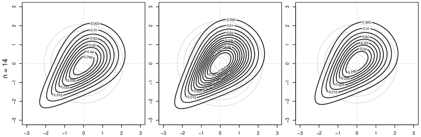
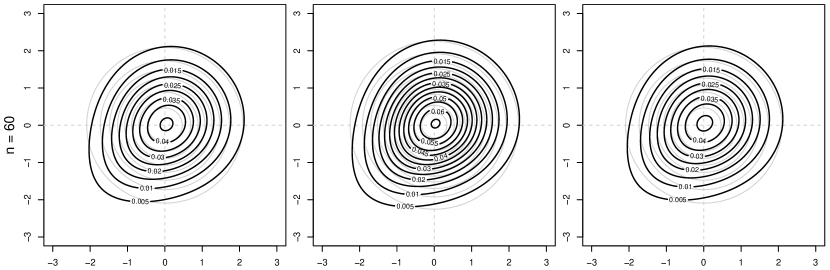
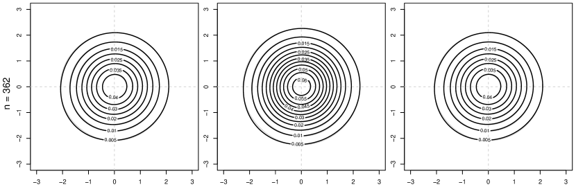
Figure 3: Two-dimensional slices of the copula density for block-maxima of the water level differences for one day, one week, one month and one winter with normalized margins.

Similar to the examples from above we see that with increasing $n$ the observed dependence structure tends to the independence copula (gray contours in the background). In case of the considered rivers this means that the maximal differences of the 12 hour average water levels over the entire winter are almost independent.

3 Copula Density of Scaled Block-Maxima

Examples 2.2 and 2.4 show that scaling of the block-maxima is necessary to achieve a limiting copula. These limiting copulas are called extreme value copulas and are characterized by max-stability. A recent introduction to extreme value copulas is given by Gudendorf and Segers (2010).

Since Hüsler and Reiss (1989) derived the scaling for the block-maxima of the multivariate normal distribution with standard normally distributed margins $X_{1},\ldots,X_{d}$ to a non-trivial extreme value copula, we use the same marginal scaling for the block-maxima $\mathbf{M}^{(n)}$ on the z-scale given by

$$W^{(n)}_{j}:=b_{n}\left(M_{j}^{(n)}-b_{n}\right),$$

where $b_{n}$ satisfies $b_{n}=n\cdot\varphi(b_{n})$ for $\varphi$ the standard normal density. Univariate extreme value theory gives that

$$F_{W^{(n)}_{j}}(w_{j})=P\left(W^{(n)}_{j}\leq w_{j}\right)=\Phi^{n}\left(b_{n}+\frac{w_{j}}{b_{n}}\right)\to\exp\{-e^{-w_{j}}\}\mbox{ as }n\to\infty$$

for $w_{j}\in\mathbb{R}$. The marginal density of $W_{j}^{(n)}$ is given by

$$f_{W^{(n)}_{j}}(w_{j})=\frac{n}{b_{n}}\Phi^{n-1}\left(b_{n}+\frac{w_{j}}{b_{n}}\right)\varphi\left(b_{n}+\frac{w_{j}}{b_{n}}\right)$$

for $w_{j}\in\mathbb{R}$, $j=1,\ldots,d$. Since $W_{j}^{(n)}$ is a strictly increasing transformation of $M_{j}^{(n)}$, the copula of $\mathbf{W}^{(n)}:=\left(W_{1}^{(n)},\ldots,W_{d}^{(n)}\right)$ is the same as the one of $\mathbf{M}^{(n)}$. Therefore, using (1.3) we obtain the following expression for the joint distribution of $\mathbf{W}^{(n)}$

$$\begin{split}F_{\mathbf{W}^{(n)}}(w_{1},\ldots,w_{d})&=P\left(W^{(n)}_{1}\leq w_{1},\ldots,W^{(n)}_{d}\leq w_{d}\right)\\ &=C_{\mathbf{M}^{(n)}}\left(\Phi^{n}\left(b_{n}+\frac{w_{1}}{b_{n}}\right),\ldots,\Phi^{n}\left(b_{n}+\frac{w_{d}}{b_{n}}\right)\right)\\ &=\left[C\left(\Phi\left(b_{n}+\frac{w_{1}}{b_{n}}\right),\ldots,\Phi\left(b_{n}+\frac{w_{d}}{b_{n}}\right)\right)\right]^{n}.\end{split}$$

Similar arguments as in Corollary 1.2 can be used to express the joint density of $\mathbf{W}^{(n)}$ in three dimensions for $n\geq 3$ as

$$\begin{split}f&{}_{\mathbf{W}^{(n)}}(w_{1},w_{2},w_{3})=\frac{1}{b_{n}^{3}}\prod_{j=1}^{d}\varphi\left(b_{n}+\frac{w_{j}}{b_{n}}\right)\Big{\{}nC\left(u_{1},u_{2},u_{3}\right)^{n-1}c\left(u_{1},u_{2},u_{3}\right)\Big{.}\\ &+n(n-1)C\left(u_{1},u_{2},u_{3}\right)^{n-2}\cdot\Big{[}\partial_{1}C\left(u_{1},u_{2},u_{3}\right)\partial_{23}C\left(u_{1},u_{2},u_{3}\right)\Big{.}\end{split}$$

$$\begin{split}\quad&+\partial_{2}C\left(u_{1},u_{2},u_{3}\right)\partial_{13}C\left(u_{1},u_{2},u_{3}\right)\Big{.}+\partial_{3}C\left(u_{1},u_{2},u_{3}\right)\partial_{12}C\left(u_{1},u_{2},u_{3}\right)\Big{]}\\ \quad&+n(n-1)(n-2)C\left(u_{1},u_{2},u_{3}\right)^{n-3}\partial_{1}C\left(u_{1},u_{2},u_{3}\right)\\ \quad&\Big{.}\cdot\partial_{2}C\left(u_{1},u_{2},u_{3}\right)\partial_{3}C\left(u_{1},u_{2},u_{3}\right)\Big{\}},\end{split}$$ (3.7)

where $u_{j}:=\Phi\left(b_{n}+\frac{w_{j}}{b_{n}}\right)$ for $j=1,2,3$.

According to Hüsler and Reiss (1989), besides scaling the maxima $M_{1}^{(n)},\ldots,M_{d}^{(n)}$, it is also necessary to change the correlation matrix $\Sigma(n)=\left(\rho_{i,j}(n)\right)_{1\leq i,j\leq d}$ of the underlying joint distribution of standard normal random variables $X_{1},\ldots,X_{n}$, over whose i.i.d. copies $X_{i,1},\ldots,X_{i,d}$, $i=1,\ldots,n$, we take the maximum. The correlation matrices $\Sigma(n)$ have to satisfy the following condition

$$\left(1-\rho_{i,j}(n)\right)\cdot\log(n)\to\lambda_{i,j}^{2}\mbox{ as }n\to\infty,$$ (3.8)

where $\lambda_{i,j}\in(0,\infty)$ are some constants for $1\leq i,j\leq d$, $i\neq j$ and $\lambda_{i,i}=0$ for $i=1,\ldots,d$. Since $\rho_{i,j}(n)=\rho_{j,i}(n)$, we also have $\lambda_{i,j}=\lambda_{j,i}$ for $1\leq i,j\leq d$. Note that (3.8) implies that $\rho_{i,j}(n)\to 1$ as $n\to\infty$. The limiting distribution $H_{\Lambda}$ of the scaled maxima depends on $\Lambda:=\left(\lambda_{i,j}\right)_{1\leq i,j\leq d}$.

In the following we will examine the three-dimensional case and choose values for $\lambda_{12},\lambda_{13},\lambda_{23}\in(0,\infty)$. For simplicity, we set

$$\rho_{i,j}(n):=1-\frac{\lambda_{i,j}^{2}}{\log(n)}$$ (3.9)

for $1\leq i,j\leq 3$, $n\in\mathbb{N}$, such that Equation 3.8 is always satisfied. However, for arbitrary $\lambda_{i,j}$ it is not trivial to decide whether we obtain a valid correlation matrix through this particular choice of $\rho_{i,j}(n)$ for any $n\in\mathbb{N}$. By construction the matrices

$$\Sigma(n)=\begin{pmatrix}1&\rho_{12}(n)&\rho_{13}(n)\\ \rho_{12}(n)&1&\rho_{23}(n)\\ \rho_{13}(n)&\rho_{23}(n)&1\end{pmatrix}$$

are symmetric and have ones on their diagonals. The only property we have to check is whether $\Sigma(n)$ is positive definite. For this we only need to check if the determinant of each leading principal minor is positive. Since $1>0$ and $1-\rho_{12}(n)^{2}>0$ are trivially satisfied, the only real requirement is that

$$\det(\Sigma(n))=1-\rho_{12}(n)\rho_{13}(n)\rho_{23}(n)-\rho_{12}(n)^{2}-\rho_{13}(n)^{2}-\rho_{23}(n)^{2}>0.$$

Using Equation 3.9 we obtain that $\det(\Sigma(n))>0$ if and only if

$$2(\lambda_{12}^{2}\lambda_{13}^{2}+\lambda_{12}^{2}\lambda_{23}^{2}+\lambda_{13}^{2}\lambda_{23}^{2})-(\lambda_{12}^{4}+\lambda_{13}^{4}+\lambda_{23}^{4})\\ >\frac{2\lambda_{12}^{2}\lambda_{13}^{2}\lambda_{23}^{2}}{\log(n)}.$$ (3.10)

We denote the left-hand side of Equation 3.10 by $h(\lambda_{12}^{2},\lambda_{13}^{2},\lambda_{23}^{2})$. Since the right-hand side of Equation 3.10 is always positive, it can only be satisfied if $h(\lambda_{12}^{2},\lambda_{13}^{2},\lambda_{23}^{2})>0$. If $h(\lambda_{12}^{2},\lambda_{13}^{2},\lambda_{23}^{2})>0$, then (3.10) is satisfied for all $n\in\mathbb{N}$ with

$$n\geq n^{*}:=\left\lfloor\exp\left\{\frac{2\lambda_{12}^{2}\lambda_{13}^{2}\lambda_{23}^{2}}{h(\lambda_{12}^{2},\lambda_{13}^{2},\lambda_{23}^{2})}\right\}+1\right\rfloor,$$

where $\left\lfloor\cdot\right\rfloor$ denotes the floor function. Table 1 shows the values of $h$ and $n^{*}$ (if existing) for 10 different combinations of $\lambda_{12},\lambda_{13},\lambda_{23}$.

#	$\lambda_{12}^{2}$	$\lambda_{13}^{2}$	$\lambda_{23}^{2}$	$h(\lambda_{12}^{2},\lambda_{13}^{2},\lambda_{23}^{2})$	$n^{*}$
1	1	1	1	3	2
2	2	2	2	12	4
3	1	2	3	8	5
4	0.5	0.5	0.5	0.75	2
5	0.3	0.2	0.1	0.08	2
6	0.2	5	0.75	-15.8	–
7	15	20	15	800	76880
8	100	0.1	20	-6376.01	–
9	1.05	0.21	0.84	0.71	2
10	4	3	3	32	10

Table 1: Different $\lambda$-combinations and the corresponding values of $h$ and $n^{*}$.

Hüsler and Reiss (1989) derived this scaling for multivariate normal distributions. Since we want to apply the scaling to vines, we need to transform the parameters of the normal distribution (correlations) to the parameters of the vine.

Considering the vine structure from (2.6) we further assume that the pair-copulas are one-parametric. Having fixed $\lambda_{12},\lambda_{13},\lambda_{23}$ such that $h(\lambda_{12}^{2},\lambda_{13}^{2},\lambda_{23}^{2})>0$, we can perform the following procedure for $n\geq n^{*}$:

1. Calculate $\rho_{12}(n)$, $\rho_{13}(n)$ and $\rho_{23}(n)$ with the help of (3.9).

2. Determine the corresponding partial correlation via

   $$\rho_{13;2}(n)=\frac{\rho_{13}(n)-\rho_{12}(n)\rho_{23}(n)}{\sqrt{1-\rho_{12}(n)^{2}}\sqrt{1-\rho_{23}(n)^{2}}}.$$

3. Translate the (partial) correlations $\rho_{12}(n)$, $\rho_{23}(n)$ and $\rho_{13;2}(n)$ into (partial) Kendall’s $\tau$ values $\tau_{12}(n)$, $\tau_{23}(n)$ and $\tau_{13;2}(n)$ using the relation for elliptical distributions

   $$\tau=\frac{2}{\pi}\arcsin(\rho).$$

4. Determine the parameters $\theta_{12}(n)$, $\theta_{13}(n)$ and $\theta_{23}(n)$ of the pair copulas from the corresponding $\tau$ values.

Recall that $\rho_{12}(n)\to 1$, $\rho_{13}(n)\to 1$ and $\rho_{23}(n)\to 1$ as $n\to\infty$. Therefore, we also have $\tau_{12}(n)\to 1$, $\tau_{13}(n)\to 1$ and $\tau_{23}(n)\to 1$ as $n\to\infty$. However, the behavior of convergence of $\rho_{13;2}(n)$ and hence $\tau_{13;2}(n)$ is not trivial. We use (3.9) to obtain

$$\begin{split}\rho_{13;2}(n)&=\frac{\left(1-\frac{\lambda_{13}^{2}}{\log(n)}\right)-\left(1-\frac{\lambda_{12}^{2}}{\log(n)}\right)\left(1-\frac{\lambda_{23}^{2}}{\log(n)}\right)}{\sqrt{1-\left(1-\frac{\lambda_{12}^{2}}{\log(n)}\right)^{2}}\sqrt{1-\left(1-\frac{\lambda_{23}^{2}}{\log(n)}\right)^{2}}}\to\frac{\lambda_{12}^{2}+\lambda_{23}^{2}-\lambda_{13}^{2}}{2\lambda_{12}\lambda_{23}}\end{split}$$

as $n\to\infty$. Thus,

$$\tau_{13;2}(n)\to\frac{2}{\pi}\arcsin\left(\frac{\lambda_{12}^{2}+\lambda_{23}^{2}-\lambda_{13}^{2}}{2\lambda_{12}\lambda_{23}}\right)\mbox{ as }n\to\infty.\\$$

For illustration, we will now take combinations 9 and 10 from Table 1. We show the (partial) correlations from Step 2 of the above procedure as well as the (partial) Kendall’s $\tau$ values since they can be compared independently from the choice the respective pair-copulas.

	$n$	$\rho_{12}(n)$	$\rho_{23}(n)$	$\rho_{13;2}(n)$	$\tau_{12}(n)$	$\tau_{23}(n)$	$\tau_{13;2}(n)$
Combination 9	10	0.54	0.64	0.87	0.37	0.44	0.67
	50	0.73	0.79	0.88	0.52	0.57	0.69
	$10^{3}$	0.85	0.88	0.89	0.64	0.68	0.69
	$\infty$	1	1	0.89	1	1	0.70
Combination 10	10	-0.74	-0.30	-0.82	-0.53	-0.20	-0.61
	50	-0.02	0.23	0.25	-0.01	0.15	0.16
	$10^{3}$	0.42	0.57	0.44	0.28	0.38	0.29
	$\infty$	1	1	0.58	1	1	0.39

Table 2: Overview over the (partial) correlations and (partial) Kendall’s $\tau$ values for different $n$ for combinations 9 ($\lambda_{12}^{2}=1.05$, $\lambda_{13}^{2}=0.21$, $\lambda_{23}^{2}=0.84$) and 10 ($\lambda_{12}^{2}=4$, $\lambda_{13}^{2}=3$, $\lambda_{23}^{2}=3$).

If we compare the values from Table 2 for combinations 9 and 10, it is eye-catching that the choice of $\lambda_{12}$, $\lambda_{13}$ and $\lambda_{23}$ has a crucial influence on the behavior of the (partial) correlations and the (partial) Kendall’s $\tau$ values. In the first case the parameters are already relatively close to their limiting values for $n=10^{3}$, whereas in the second case they are still rather far from their limits for $n=10^{3}$. Further, we see that the limiting values of $\rho_{13;2}(n)$ and $\tau_{13;2}(n)$ can be very different depending on the choice $\lambda_{12}$, $\lambda_{13}$ and $\lambda_{23}$.

Now we examine the behavior of the three-dimensional density of the scaled block-maxima $f_{\mathbf{W}^{(n)}}$ for increasing values of $n$.

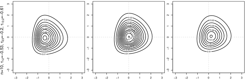
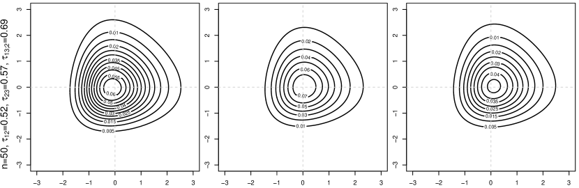
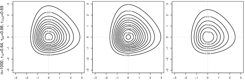
Figure 4: Two-dimensional slices of the density of the scaled block-maxima of a three-dimensional Clayton-vine ($\lambda_{12}^{2}=1.05$, $\lambda_{13}^{2}=0.21$, $\lambda_{23}^{2}=0.84$).

Example 3.1.

First we look at a Clayton-vine and choose $\lambda_{12}^{2}=1.05$, $\lambda_{13}^{2}=0.21$ and $\lambda_{23}^{2}=0.84$ (combination 9). The parameters and Kendall’s $\tau$ values depend on the block-size $n$.

Figure 4 shows the density of the scaled block-maxima of the Clayton-vine for block-sizes $n=10$, $50$, $10^{3}$. Each row represents one block-size (and thus parameter set) and contains three contour plots corresponding to z₃-values fixed to $F_{W_{3}^{(n)}}^{-1}(0.2)$, $F_{W_{3}^{(n)}}^{-1}(0.5)$ or $F_{W_{3}^{(n)}}^{-1}(0.8)$, respectively.

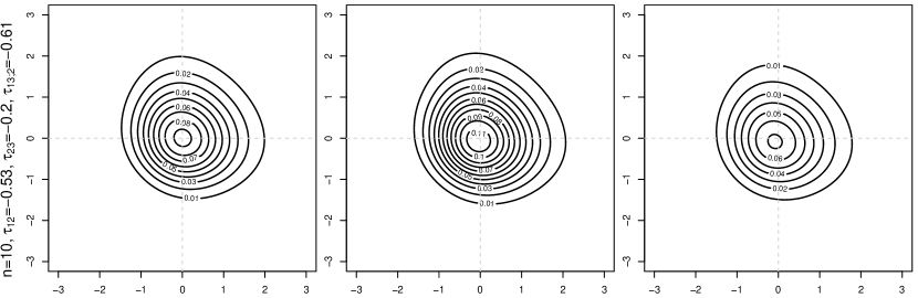
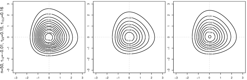
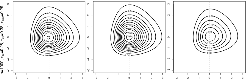
Figure 5: Two-dimensional slices of the density of the scaled block-maxima of a three-dimensional Gaussian vine ($\lambda_{12}^{2}=4$, $\lambda_{13}^{2}=3$, $\lambda_{23}^{2}=3$).

Example 3.2.

As a second example we choose a Gaussian vine with $\lambda_{12}^{2}=4$, $\lambda_{13}^{2}=3$ and $\lambda_{23}^{2}=3$ (combination 10).

Figure 5 shows the density of the scaled block-maxima of the Gaussian vine for block-sizes $n=10$, $50$, $10^{3}$. Again, three contour plots corresponding to z₃-values fixed to $F_{W_{3}^{(n)}}^{-1}(0.2)$, $F_{W_{3}^{(n)}}^{-1}(0.5)$ or $F_{W_{3}^{(n)}}^{-1}(0.8)$, respectively, are displayed per row. The block-size and Kendall’s $\tau$ values are denoted on the left for each row.

Conclusion

In this chapter we showed that the copula density of the block-maxima of multivariate distributions can be expressed explicitly. For three-dimensional vine copulas we made use of the fact that we can compute their partial derivatives by one-dimensional integration, which makes the evaluation of the copula density for block-maxima numerically tractable. The advantage of our method is that we can use the entire sample for estimation instead of reducing the sample size by taking the maximum over $n$ observations. Once we have estimated the underlying dependence structure we can derive the copula density of the block-maxima for any block-size (even larger than the original sample size). From the Clayton and the Gauss examples we have seen that without proper scaling the block-maxima do not approach a non-trivial limiting distribution for increasing block-size.

Appendix

Proof of Theorem 1.1

In order to prove Theorem 1.1 we prove an auxiliary lemma from which Theorem 1.1 follows as a corollary.

Lemma 3.3.

For $k\in\left\{1,\ldots,d\right\}$ and $u_{j}\in[0,1]$, $j=1\ldots,d$, we have

$$\frac{\partial^{k}}{\partial u_{1}\cdots\partial u_{k}}\left[C(u_{1}^{1/n},\ldots,u_{d}^{1/n})^{n}\right]=\frac{1}{n^{k}}\left(\prod_{j=1}^{k}u_{j}\right)^{\frac{1}{n}-1}\\ \cdot\sum_{j=1}^{k\wedge n}\left\{\frac{n!}{(n-j)!}\cdot C\left(u_{1}^{1/n},\ldots,u_{d}^{1/n}\right)^{n-j}\sum_{\mathcal{P}\in\mathcal{S}_{k,j}}\prod_{M\in\mathcal{P}}\partial_{M}C\left(u_{1}^{1/n},\ldots,u_{d}^{1/n}\right)\right\}.$$

Proof.

We will prove this statement using induction. For $k=1$ we have

$$\frac{\partial}{\partial u_{1}}\left[C(u_{1}^{1/n},\ldots,u_{d}^{1/n})^{n}\right]=nC(u_{1}^{1/n},\ldots,u_{d}^{1/n})^{n-1}\partial_{1}C(u_{1}^{1/n},\ldots,u_{d}^{1/n})\frac{1}{n}u_{1}^{\frac{1}{n}-1}=\\ \frac{1}{n^{1}}\left(\prod_{j=1}^{1}u_{j}\right)^{\frac{1}{n}-1}\sum_{j=1}^{1\wedge n}\left\{\frac{n!}{(n-j)!}C(u_{1}^{1/n},\ldots,u_{d}^{1/n})^{n-j}\sum_{\mathcal{P}\in\mathcal{S}_{1,j}}\prod_{M\in\mathcal{P}}\partial_{M}C(u_{1}^{1/n},\ldots,u_{d}^{1/n})\right\}.$$

The inductive step ($k\to k+1$) proceeds as follows

$$\frac{\partial^{k+1}}{\partial u_{1}\cdots\partial u_{k+1}}\left[C(u_{1}^{1/n},\ldots,u_{d}^{1/n})^{n}\right]=\frac{\partial}{\partial u_{k+1}}\left\{\frac{\partial^{k}}{\partial u_{1}\cdots\partial u_{k}}\left[C(u_{1}^{1/n},\ldots,u_{d}^{1/n})^{n}\right]\right\}=:\left(*\right)_{1}.$$

Applying the inductive assumption yields

$$\left(*\right)_{1}=\frac{\partial}{\partial u_{k+1}}\left\{\frac{1}{n^{k}}\left(\prod_{j=1}^{k}u_{j}\right)^{\frac{1}{n}-1}\sum_{j=1}^{k\wedge n}\left\{\frac{n!}{(n-j)!}\cdot C\left(u_{1}^{1/n},\ldots,u_{d}^{1/n}\right)^{n-j}\right.\right.\\ \cdot\big{.}\big{.}\sum_{\mathcal{P}\in\mathcal{S}_{k,j}}\prod_{M\in\mathcal{P}}\partial_{M}C\left(u_{1}^{1/n},\ldots,u_{d}^{1/n}\right)\bigg{\}}\Bigg{\}}=:\left(*\right)_{2}$$

We will consider the cases ”$n>k$” and ”$n\leq k$” separately. We begin with Case 1 ($n>k$): We have $k\wedge n=k$ and hence

$$\begin{split}\left(*\right)_{2}&=\frac{1}{n^{k}}\left(\prod_{j=1}^{k}u_{j}\right)^{\frac{1}{n}-1}\sum_{j=1}^{k}\Bigg{\{}\frac{n!}{(n-j)!}\cdot\left\{\frac{\partial}{\partial u_{k+1}}\left[C\left(u_{1}^{1/n},\ldots,u_{d}^{1/n}\right)^{n-j}\right]\right.\Bigg{.}\\ &\quad\cdot\big{.}\sum_{\mathcal{P}\in\mathcal{S}_{k,j}}\prod_{M\in\mathcal{P}}\partial_{M}C\left(u_{1}^{1/n},\ldots,u_{d}^{1/n}\right)+C\left(u_{1}^{1/n},\ldots,u_{d}^{1/n}\right)^{n-j}\\ &\quad\cdot\frac{\partial}{\partial u_{k+1}}\left[\sum_{\mathcal{P}\in\mathcal{S}_{k,j}}\prod_{M\in\mathcal{P}}\partial_{M}C\left(u_{1}^{1/n},\ldots,u_{d}^{1/n}\right)\right]\Bigg{\}}=\left(*\right)_{3}.\end{split}$$

Now we use that fact that for $k\in\left\{1,\ldots,d-1\right\}$ and $j\in\left\{1,\ldots,k\wedge n\right\}$ we have

$$\frac{\partial}{\partial u_{k+1}}\left[\sum_{\mathcal{P}\in\mathcal{S}_{k,j}}\prod_{M\in\mathcal{P}}\partial_{M}C\left(u_{1}^{1/n},\ldots,u_{d}^{1/n}\right)\right]=\frac{u_{k+1}^{\frac{1}{n}-1}}{n}\sum_{\begin{subarray}{c}\mathcal{P}\in\mathcal{S}_{k+1,j}\\ \left\{k+1\right\}\not\in\mathcal{P}\end{subarray}}\prod_{M\in\mathcal{P}}\partial_{M}C\left(u_{1}^{1/n},\ldots,u_{d}^{1/n}\right).$$ (3.11)

Applying Equation 3.11 yields

$$\begin{split}\left(*\right)_{3}&=\frac{1}{n^{k}}\left(\prod_{j=1}^{k}u_{j}\right)^{\frac{1}{n}-1}\Bigg{\{}\sum_{j=1}^{k}\frac{n!}{(n-j)!}\cdot(n-j)\cdot C\left(u_{1}^{1/n},\ldots,u_{d}^{1/n}\right)^{n-j-1}\Bigg{.}\\ &\quad\cdot\partial_{k+1}C\left(u_{1}^{1/n},\ldots,u_{d}^{1/n}\right)\frac{1}{n}u_{k+1}^{\frac{1}{n}-1}\cdot\sum_{\mathcal{P}\in\mathcal{S}_{k,j}}\prod_{M\in\mathcal{P}}\partial_{M}C\left(u_{1}^{1/n},\ldots,u_{d}^{1/n}\right)\\ &\quad\big{.}+\sum_{j=1}^{k}\frac{n!}{(n-j)!}\cdot C\left(u_{1}^{1/n},\ldots,u_{d}^{1/n}\right)^{n-j}\cdot\frac{1}{n}u_{k+1}^{\frac{1}{n}-1}\sum_{\begin{subarray}{c}\mathcal{P}\in\mathcal{S}_{k+1,j}\\ \left\{k+1\right\}\not\in\mathcal{P}\end{subarray}}\prod_{M\in\mathcal{P}}\partial_{M}C\left(u_{1}^{1/n},\ldots,u_{d}^{1/n}\right)\Bigg{\}}\\ &=\frac{1}{n^{k+1}}\left(\prod_{j=1}^{k+1}u_{j}\right)^{\frac{1}{n}-1}\Bigg{\{}\sum_{j=1}^{k}\frac{n!}{(n-(j+1))!}\cdot C\left(u_{1}^{1/n},\ldots,u_{d}^{1/n}\right)^{n-(j+1)}\Bigg{.}\\ &\quad\cdot\sum_{\begin{subarray}{c}\mathcal{P}\in\mathcal{S}_{k+1,j+1}\\ \left\{k+1\right\}\in\mathcal{P}\end{subarray}}\prod_{M\in\mathcal{P}}\partial_{M}C\left(u_{1}^{1/n},\ldots,u_{d}^{1/n}\right)\\ &\quad\big{.}+\sum_{j=1}^{k}\frac{n!}{(n-j)!}\cdot C\left(u_{1}^{1/n},\ldots,u_{d}^{1/n}\right)^{n-j}\cdot\sum_{\begin{subarray}{c}\mathcal{P}\in\mathcal{S}_{k+1,j}\\ \left\{k+1\right\}\not\in\mathcal{P}\end{subarray}}\prod_{M\in\mathcal{P}}\partial_{M}C\left(u_{1}^{1/n},\ldots,u_{d}^{1/n}\right)\Bigg{\}}=\left(*\right)_{4}.\\ \end{split}$$

We perform an index shift in the first sum such that $j+1$ is replaced by $j$ and make use of the following two properties:

• For all $\mathcal{P}\in\mathcal{S}_{l,1}=\left\{\left\{\left\{1,\ldots,l\right\}\right\}\right\}$ holds that $\left\{l\right\}\not\in\mathcal{P}$.

• For all $\mathcal{P}\in\mathcal{S}_{l,l}=\left\{\left\{\left\{1\right\},\ldots,\left\{l\right\}\right\}\right\}$ holds that $\left\{l\right\}\in\mathcal{P}$.

This results in

$$\begin{split}\left(*\right)_{4}&=\frac{1}{n^{k+1}}\left(\prod_{j=1}^{k+1}u_{j}\right)^{\frac{1}{n}-1}\Bigg{\{}\sum_{j=1}^{k+1}\frac{n!}{(n-j)!}\cdot C\left(u_{1}^{1/n},\ldots,u_{d}^{1/n}\right)^{n-j}\Bigg{.}\\ &\quad\cdot\sum_{\begin{subarray}{c}\mathcal{P}\in\mathcal{S}_{k+1,j}\\ \left\{k+1\right\}\in\mathcal{P}\end{subarray}}\prod_{M\in\mathcal{P}}\partial_{M}C\left(u_{1}^{1/n},\ldots,u_{d}^{1/n}\right)\\ &\quad\big{.}+\sum_{j=1}^{k+1}\frac{n!}{(n-j)!}\cdot C\left(u_{1}^{1/n},\ldots,u_{d}^{1/n}\right)^{n-j}\cdot\sum_{\begin{subarray}{c}\mathcal{P}\in\mathcal{S}_{k+1,j}\\ \left\{k+1\right\}\not\in\mathcal{P}\end{subarray}}\prod_{M\in\mathcal{P}}\partial_{M}C\left(u_{1}^{1/n},\ldots,u_{d}^{1/n}\right)\Bigg{\}}\\ &=\frac{1}{n^{k+1}}\left(\prod_{j=1}^{k+1}u_{j}\right)^{\frac{1}{n}-1}\Bigg{\{}\sum_{j=1}^{(k+1)\wedge n}\frac{n!}{(n-j)!}\cdot C\left(u_{1}^{1/n},\ldots,u_{d}^{1/n}\right)^{n-j}\Bigg{.}\\ &\quad\cdot\Bigg{.}\sum_{\mathcal{P}\in\mathcal{S}_{k+1,j}}\prod_{M\in\mathcal{P}}\partial_{M}C\left(u_{1}^{1/n},\ldots,u_{d}^{1/n}\right)\Bigg{\}},\end{split}$$

where we used the fact that $k+1=(k+1)\wedge n$ since $n>k$. This concludes the first case. Case 2 ($n\leq k$) is similar to the first one. The main difference is that $C\left(u_{1}^{1/n},\ldots,u_{d}^{1/n}\right)^{n-j}=1$ for $j=n$, which was not possible before since $j\leq k<n$. Now $k\wedge n=n$ and therefore we obtain

$$\begin{split}\left(*\right)_{2}&=\frac{1}{n^{k}}\left(\prod_{j=1}^{k}u_{j}\right)^{\frac{1}{n}-1}\Bigg{\{}\sum_{j=1}^{n-1}\frac{n!}{(n-j)!}\cdot(n-j)\cdot C\left(u_{1}^{1/n},\ldots,u_{d}^{1/n}\right)^{n-j-1}\Bigg{.}\\ &\quad\cdot\partial_{k+1}C\left(u_{1}^{1/n},\ldots,u_{d}^{1/n}\right)\frac{1}{n}u_{k+1}^{\frac{1}{n}-1}\cdot\sum_{\mathcal{P}\in\mathcal{S}_{k,j}}\prod_{M\in\mathcal{P}}\partial_{M}C\left(u_{1}^{1/n},\ldots,u_{d}^{1/n}\right)\\ &\quad\big{.}+\sum_{j=1}^{n}\frac{n!}{(n-j)!}C\left(u_{1}^{1/n},\ldots,u_{d}^{1/n}\right)^{n-j}\frac{\partial}{\partial u_{k+1}}\left[\sum_{\mathcal{P}\in\mathcal{S}_{k,j}}\prod_{M\in\mathcal{P}}\partial_{M}C\left(u_{1}^{1/n},\ldots,u_{d}^{1/n}\right)\right]\Bigg{\}}\\ &=\frac{1}{n^{k+1}}\left(\prod_{j=1}^{k+1}u_{j}\right)^{\frac{1}{n}-1}\Bigg{\{}\sum_{j=1}^{n-1}\frac{n!}{(n-(j+1))!}\cdot C\left(u_{1}^{1/n},\ldots,u_{d}^{1/n}\right)^{n-(j+1)}\Bigg{.}\\ &\quad\cdot\sum_{\begin{subarray}{c}\mathcal{P}\in\mathcal{S}_{k+1,j+1}\\ \left\{k+1\right\}\in\mathcal{P}\end{subarray}}\prod_{M\in\mathcal{P}}\partial_{M}C\left(u_{1}^{1/n},\ldots,u_{d}^{1/n}\right)\\ &\quad\big{.}+\sum_{j=1}^{n}\frac{n!}{(n-j)!}\cdot C\left(u_{1}^{1/n},\ldots,u_{d}^{1/n}\right)^{n-j}\cdot\sum_{\begin{subarray}{c}\mathcal{P}\in\mathcal{S}_{k+1,j}\\ \left\{k+1\right\}\not\in\mathcal{P}\end{subarray}}\prod_{M\in\mathcal{P}}\partial_{M}C\left(u_{1}^{1/n},\ldots,u_{d}^{1/n}\right)\Bigg{\}}\\ &=\frac{1}{n^{k+1}}\left(\prod_{j=1}^{k+1}u_{j}\right)^{\frac{1}{n}-1}\Bigg{\{}\sum_{j=1}^{n}\frac{n!}{(n-j)!}\cdot C\left(u_{1}^{1/n},\ldots,u_{d}^{1/n}\right)^{n-j}\Bigg{.}\\ &\quad\cdot\sum_{\begin{subarray}{c}\mathcal{P}\in\mathcal{S}_{k+1,j}\\ \left\{k+1\right\}\in\mathcal{P}\end{subarray}}\prod_{M\in\mathcal{P}}\partial_{M}C\left(u_{1}^{1/n},\ldots,u_{d}^{1/n}\right)+\sum_{j=1}^{n}\frac{n!}{(n-j)!}\cdot C\left(u_{1}^{1/n},\ldots,u_{d}^{1/n}\right)^{n-j}\\ &\quad\big{.}\cdot\sum_{\begin{subarray}{c}\mathcal{P}\in\mathcal{S}_{k+1,j}\\ \left\{k+1\right\}\not\in\mathcal{P}\end{subarray}}\prod_{M\in\mathcal{P}}\partial_{M}C\left(u_{1}^{1/n},\ldots,u_{d}^{1/n}\right)\Bigg{\}}\end{split}$$

$$\begin{split}\quad&=\frac{1}{n^{k+1}}\left(\prod_{j=1}^{k+1}u_{j}\right)^{\frac{1}{n}-1}\Bigg{\{}\sum_{j=1}^{(k+1)\wedge n}\frac{n!}{(n-j)!}\cdot C\left(u_{1}^{1/n},\ldots,u_{d}^{1/n}\right)^{n-j}\Bigg{.}\\ \quad&\quad\cdot\Bigg{.}\sum_{\mathcal{P}\in\mathcal{S}_{k+1,j}}\prod_{M\in\mathcal{P}}\partial_{M}C\left(u_{1}^{1/n},\ldots,u_{d}^{1/n}\right)\Bigg{\}},\end{split}$$

where we applied Equation 3.11 in the second equality. In the third equality we performed an index shift in the first sum and used property (a) above. Since $n\leq k$ we have $n=(k+1)\wedge n$. This concludes the second case and hence the proof of Lemma 3.3. ∎

Having proved the auxiliary lemma we can now easily prove the statement from Theorem 1.1.

Proof of Theorem 1.1.

Using Equation 1.3 we obtain

$$\begin{split}c_{\mathbf{M}^{(n)}}(u_{1},\ldots,u_{d})&=\frac{\partial^{d}}{\partial u_{1}\cdots\partial u_{d}}C_{\mathbf{M}^{(n)}}(u_{1},\ldots,u_{d})=\frac{\partial^{d}}{\partial u_{1}\cdots\partial u_{d}}\left[C(u_{1}^{1/n},\ldots,u_{d}^{1/n})^{n}\right].\end{split}$$

Now Theorem 1.1 follows directly from Lemma 3.3 for $k=d$. ∎

Proof of Theorem 2.1

Proof.

Expression 4) follows directly by the definition of $c(u_{1},u_{2},u_{3})$ (see Equation 2.6). For expression 3(a) we can write

$$\begin{split}\partial_{23}C(u_{1},&u_{2},u_{3})\stackrel{{\scriptstyle Eq.(\ref{eq:pcc})}}{{=}}c_{23}(u_{2},u_{3})\int_{0}^{u_{1}}c_{12}(v_{1},u_{2})c_{13;2}(C_{1|2}(v_{1}|u_{2}),C_{3|2}(u_{3}|u_{2}))dv_{1}\\ &=c_{23}(u_{2},u_{3})\int_{0}^{u_{1}}\partial_{12}C_{12}(v_{1},u_{2})\partial_{13}C_{13;2}(C_{1|2}(v_{1}|u_{2}),C_{3|2}(u_{3}|u_{2}))dv_{1}\\ &=c_{23}(u_{2},u_{3})\int_{0}^{u_{1}}\frac{\partial}{\partial v_{1}}\bigg{[}\underbrace{\partial_{2}C_{12}(v_{1},u_{2})}_{C_{1|2}(v_{1}|u_{2})=w_{1}}\bigg{]}\partial_{13}C_{13;2}(C_{1|2}(v_{1}|u_{2}),C_{3|2}(u_{3}|u_{2}))dv_{1}\\ &=c_{23}(u_{2},u_{3})\int_{0}^{u_{1}}\frac{\partial w_{1}}{\partial v_{1}}\frac{\partial}{\partial w_{1}}\partial_{3}C_{13;2}(w_{1},C_{3|2}(u_{3}|u_{2}))\bigg{|}_{\begin{subarray}{c}w_{1}=C_{1|2}(v_{1}|u_{2})\end{subarray}}dv_{1}\\ &=c_{23}(u_{2},u_{3})\partial_{3}C_{13;2}(C_{1|2}(u_{1}|u_{2}),C_{3|2}(u_{3}|u_{2})).\end{split}$$

Expression 3(a) follows similarly. For expression 2(c) we have

$$\begin{split}\partial_{3}C(u_{1},u_{2},u_{3})&=\int_{0}^{u_{1}}\int_{0}^{u_{2}}c(v_{1},v_{2},u_{3})dv_{1}dv_{2}\\ &=\int_{0}^{u_{2}}c_{23}(v_{2},u_{3})C_{1|23}(u_{1}|v_{2},u_{3})dv_{2}\\ &=\int_{0}^{u_{2}}c_{23}(v_{2},u_{3})\partial_{3}C_{13;2}(C_{1|2}(u_{1}|v_{2}),C_{3|2}(u_{3}|v_{2}))dv_{2}.\end{split}$$

Further, $\partial_{3}C(u_{1},u_{2},u_{3})$ can be written in another way which we use for the calculation of the copula $C(u_{1},u_{2},u_{3})$. In particular we have

$$\begin{split}\partial_{3}C&(u_{1},u_{2},u_{3})=\int_{0}^{u_{1}}\int_{0}^{u_{2}}c(v_{1},v_{2},u_{3})dv_{1}dv_{2}\\ &=\int_{0}^{u_{2}}\frac{\partial^{2}}{\partial v_{2}\partial u_{3}}C_{23}(v_{2},u_{3})\frac{\partial}{\partial w_{2}}C_{13;2}(C_{1|2}(u_{1}|v_{2}),w_{2})\bigg{|}_{w_{2}=C_{3|2}(u_{3}|v_{2})}dv_{2}\\ &=\int_{0}^{u_{2}}\frac{\partial w_{2}}{\partial u_{3}}\frac{\partial}{\partial w_{2}}C_{13;2}(C_{1|2}(u_{1}|v_{2}),w_{2})\bigg{|}_{w_{2}=C_{3|2}(u_{3}|v_{2})}dv_{2}\\ &=\int_{0}^{u_{2}}\frac{\partial}{\partial u_{3}}C_{13;2}(C_{1|2}(u_{1}|v_{2}),C_{3|2}(u_{3}|v_{2}))dv_{2}\\ &=\frac{\partial}{\partial u_{3}}\left[\int_{0}^{u_{2}}C_{13;2}(C_{1|2}(u_{1}|v_{2}),C_{3|2}(u_{3}|v_{2}))dv_{2}\right].\end{split}$$ (3.12)

Similarly one can derive expression 2(a). For the copula in expression 1 we have

$$\begin{split}C(u_{1},u_{2},u_{3})&\stackrel{{\scriptstyle\eqref{eq:d3C}}}{{=}}\int_{0}^{u_{3}}\frac{\partial}{\partial v_{3}}\left[\int_{0}^{u_{2}}C_{13;2}(C_{1|2}(u_{1}|v_{2}),C_{3|2}(v_{3}|v_{2}))dv_{2}\right]dv_{3}\\ &=\int_{0}^{u_{2}}\left[\int_{0}^{u_{3}}\frac{\partial}{\partial v_{3}}C_{13;2}(C_{1|2}(u_{1}|v_{2}),C_{3|2}(v_{3}|v_{2}))dv_{3}\right]dv_{2}\\ &=\int_{0}^{u_{2}}C_{13;2}\left(C_{1|2}(u_{1}|v_{2}),C_{3|2}(u_{3}|v_{2})\right)dv_{2}.\end{split}$$

Expression 2(b) follows by differentiating expression 1 with respect to $v_{2}$. It remains to show expression 3(b). For this we differentiate 2(c) with respect to $v_{1}$. Therefore we have

$$\begin{split}\partial_{13}C(u_{1},&u_{2},u_{3})=\frac{\partial}{\partial u_{1}}\left[\int_{0}^{u_{2}}\partial_{3}C_{13;2}(C_{1|2}(u_{1}|v_{2}),C_{3|2}(u_{3}|v_{2}))c_{23}(v_{2},u_{3})dv_{2}\right]\\ &=\int_{0}^{u_{2}}\partial_{13}C_{13;2}(C_{1|2}(u_{1}|v_{2}),C_{3|2}(u_{3}|v_{2}))c_{12}(u_{1},v_{2})c_{23}(v_{2},u_{3})dv_{2}\\ &=\int_{0}^{u_{2}}c_{13;2}(C_{1|2}(u_{1}|v_{2}),C_{3|2}(u_{3}|v_{2}))c_{12}(u_{1},v_{2})c_{23}(v_{2},u_{3})dv_{2}.\end{split}$$

∎

References

- Aas et al. (2009) Aas, K., Czado, C., Frigessi, A., and Bakken, H. (2009), “Pair-copula constructions of multiple dependence,” Insurance, Mathematics and Economics, 44, 182–198.
- Bedford and Cooke (2002) Bedford, T. and Cooke, R. M. (2002), “Vines - a new graphical model for dependent random variables,” Annals of Statistics, 30, 1031–1068.
- Bücher and Segers (2013) Bücher, A. and Segers, J. (2013), “Extreme value copula estimation based on block maxima of a multivariate stationary time series,” arXiv preprint arXiv:1311.3060.
- Czado (2010) Czado, C. (2010), “Pair-copula constructions of multivariate copulas,” In F. Durante, W. Härdle, P. Jaworki, and T. Rychlik (Eds.), Workshop on Copula Theory and its Applications. Springer, Dordrecht.
- Czado et al. (2013) Czado, C., Brechmann, E., and Gruber, L. (2013), “Selection of Vine Copulas,” in Copulae in Mathematical and Quantitative Finance, eds. P. Jaworski, F. D. and Härdle, W. K., Springer.
- Dombry (2013) Dombry, C. (2013), “Maximum likelihood estimators for the extreme value index based on the block maxima method,” arXiv preprint arXiv:1301.5611.
- Faranda et al. (2011) Faranda, D., Lucarini, V., Turchetti, G., and Vaienti, S. (2011), “Numerical convergence of the block-maxima approach to the Generalized Extreme Value distribution,” Journal of statistical physics, 145, 1156–1180.
- Ferreira et al. (2014) Ferreira, A., de Haan, L., et al. (2014), “On the block maxima method in extreme value theory: PWM estimators,” The Annals of Statistics, 43, 276–298.
- Gudendorf and Segers (2010) Gudendorf, G. and Segers, J. (2010), “Extreme-value copulas,” in Copula theory and its applications, Springer, pp. 127–145.
- Hüsler and Reiss (1989) Hüsler, J. and Reiss, R.-D. (1989), “Maxima of normal random vectors: between independence and complete dependence,” Statistics & Probability Letters, 7, 283–286.
- Jarušková and Hanek (2006) Jarušková, D. and Hanek, M. (2006), “Peaks over threshold method in comparison with block-maxima method for estimating high return levels of several Northern Moravia precipitation and discharges series,” Journal of Hydrology and Hydromechanics, 54, 309–319.
- Joe (1997) Joe, H. (1997), Multivariate Models and Dependence Concepts, London: Chapman & Hall.
- Kurowicka and Cooke (2006) Kurowicka, D. and Cooke, R. (2006), Uncertainty analysis with high dimensional dependence modelling, Chichester: Wiley.
- Kurowicka and Joe (2011) Kurowicka, D. and Joe, H. (2011), Dependence Modeling - Handbook on Vine Copulae, Singapore: World Scientific Publishing Co.
- Marty and Blanchet (2012) Marty, C. and Blanchet, J. (2012), “Long-term changes in annual maximum snow depth and snowfall in Switzerland based on extreme value statistics,” Climatic Change, 111, 705–721.
- McNeil et al. (2010) McNeil, A. J., Frey, R., and Embrechts, P. (2010), Quantitative risk management: concepts, techniques, and tools, Princeton university press.
- Naveau et al. (2009) Naveau, P., Guillou, A., Cooley, D., and Diebolt, J. (2009), “Modelling pairwise dependence of maxima in space,” Biometrika, 96, 1–17.
- Nikulin et al. (2011) Nikulin, G., Kjellström, E., Hansson, U., Strandberg, G., and Ullerstig, A. (2011), “Evaluation and future projections of temperature, precipitation and wind extremes over Europe in an ensemble of regional climate simulations,” Tellus A, 63, 41–55.
- Rocco (2014) Rocco, M. (2014), “Extreme value theory in finance: A survey,” Journal of Economic Surveys, 28, 82–108.
- Schepsmeier et al. (2014) Schepsmeier, U., Stoeber, J., Brechmann, E. C., and Graeler, B. (2014), VineCopula: Statistical inference of vine copulas, R package version 1.3/r66.
- Sklar (1959) Sklar, A. (1959), “Fonctions dé Repartition á n Dimensions et leurs Marges,” Publ. Inst. Stat. Univ. Paris, 8, 229–231.
- Stöber and Czado (2012) Stöber, J. and Czado, C. (2012), “Pair Copula Constructions,” in Simulating Copulas: Stochastic Models, Sampling Algorithms, and Applications, eds. Mai, J. and Scherer, M., Imperial College Press.
- Stöber et al. (2013) Stöber, J., Joe, H., and Czado, C. (2013), “Simplified pair copula constructions – Limitations and extensions,” Journal of Multivariate Analysis, 119, 101 – 118.