Jacobi stability analysis of the Lorenz system

Abstract

We perform the study of the stability of the Lorenz system by using the Jacobi stability analysis, or the Kosambi-Cartan-Chern (KCC) theory. The Lorenz model plays an important role for understanding hydrodynamic instabilities and the nature of the turbulence, also representing a non-trivial testing object for studying non-linear effects. The KCC theory represents a powerful mathematical method for the analysis of dynamical systems. In this approach we describe the evolution of the Lorenz system in geometric terms, by considering it as a geodesic in a Finsler space. By associating a non-linear connection and a Berwald type connection, five geometrical invariants are obtained, with the second invariant giving the Jacobi stability of the system. The Jacobi (in)stability is a natural generalization of the (in)stability of the geodesic flow on a differentiable manifold endowed with a metric (Riemannian or Finslerian) to the non-metric setting. In order to apply the KCC theory we reformulate the Lorenz system as a set of two second order non-linear differential equations. The geometric invariants associated to this system (nonlinear and Berwald connections), and the deviation curvature tensor, as well as its eigenvalues, are explicitly obtained. The Jacobi stability of the equilibrium points of the Lorenz system is studied, and the condition of the stability of the equilibrium points is obtained. Finally, we consider the time evolution of the components of the deviation vector near the equilibrium points.

I Introduction

Continuously time evolving dynamical systems are one of the basic theoretical tools for modeling the evolution of natural phenomena in every branch of physics, chemistry, or biology. Their usefulness in scientific/engineering applications is determined by their predictive power, which, in turn, strongly depends on the stability of their solutions. Since in the measured initial conditions in a physical system some uncertainty inevitably does exist, a physically meaningful mathematical model must offer an understanding of the possible evolution of the deviations of the trajectories of the studied dynamical system from a given reference trajectory. Note that a local understanding of the stability is as important as the global evolution and control of late-time deviations. From a mathematical point of view the global stability of the solutions of the dynamical systems is described by the well studied theory of Lyapounov stability. In this approach the fundamental quantities are the Lyapunov exponents, measuring exponential deviations from the given trajectory 1 ; 2 . It is usually very difficult to analytically determine the Lyapounov exponents, and therefore various numerical methods for their calculation have been proposed, and are used in various situations 3 -11 . On the other hand the local stability of solutions of dynamical systems is much less understood.

Even that the methods of the Lyapounov stability analysis are well established, it would be interesting to study the stability of the dynamical system from different points of view, and to compare the results with the corresponding Lyapunov exponents analysis. Such an alternative approach to the study of the dynamical systems is represented by the so-called geometrodynamical approach, which was initiated in the pioneering work of Kosambi Ko33 , Cartan Ca33 and Chern Ch39 . The Kosambi-Cartan-Chern (KCC) approach is inspired by the geometry of the Finsler spaces. Its basic idea is to consider that there is a one to one correspondence between a second order dynamical system and the geodesic equations in an associated Finsler space (for a recent review of the KCC theory see rev ). The KCC theory is a differential geometric theory of the variational equations for the deviations of the whole trajectory to nearby ones An00 . In this geometrical description of the dynamical systems one associates a non-linear connection, and a Berwald type connection to the differential system, and five geometrical invariants are obtained. The second invariant, also called the curvature deviation tensor, gives the Jacobi stability of the system rev ; An00 ; Sa05 ; Sa05a . The KCC theory has been applied for the study of different physical, biochemical or technical systems (see Sa05 ; Sa05a ; An93 ; YaNa07 ; Ha1 ; Ha2 ).

An alternative geometrization method for dynamical systems was proposed in Pet1 and Kau , and further investigated in Pet0 -Pet4 . Specific applications for the Henon-Heiles system and Bianchi type IX cosmological models were also considered. In particular, in Pet0 a theoretical framework devoted to a geometrical description of the behavior of dynamical systems and their chaotic properties was developed.

In the Riemmannian geometric approach to dynamical systems one starts with the well-known results that the flow associated with a time dependent Hamiltonian $H=\delta^{ab}p_{a}p_{b}/2+V\left(x^{a}\right)$ can be reformulated as a geodesic flow in a curved, but conformally flat, manifold Kau . By introducing a metric of the form $ds^{2}=W\left(x^{a}\right)\delta_{ab}dx^{a}dx^{b}$, with the conformal factor given by $W\left(x^{a}\right)=E-V\left(x^{a}\right)$, where $E$ is the conserved energy associated with the time-independent $H$, it follows that the geodesic equation for motion in the metric $g_{ab}=W\left(x^{a}\right)\delta_{ab}$ is completely equivalent to the Hamilton equations $dx^{a}/dt=\partial H/\partial p_{a}$, $dp_{a}/dt=-\partial H/\partial x_{a}$ Kau . This implies that the confluence or divergence of nearby trajectories $x^{a}(s)$ and $[x+\xi]^{a}(s)$ is determined by the Jacobi equation, i.e., the equation of geodesic deviation, which takes the form

$$\frac{D^{2}\xi^{a}}{Ds^{2}}=−R^{a}_{bcd}u^{b}u^{d}\xi^{c}\equiv-K^{a}_{c}\xi^{c},$$ (1)

where $R^{a}_{bcd}$ is the Riemann tensor associated with $g_{ab}$, and $D/Ds=u^{a}\nabla_{a}$ denotes a directional derivative along $u^{a}=dx^{a}/ds$. Linear stability for the trajectory $x^{a}(s)$ is thus related to $R^{a}_{bcd}$ or, more exactly, to the curvature $K^{a}_{c}$. If, for example, $R^{a}_{bcd}$ is everywhere negative, so that $K^{a}_{c}$ always has one or more negative eigenvalues, the trajectory must be linearly unstable Kau .

The global and local stability of solutions of continuously evolving dynamical systems was reconsidered, from a geometric perspective, in Punzi . It was shown that an unambiguous definition of stability generally requires the choice of additional geometric structures that are not intrinsic to the dynamical system itself.

One of the most studied non-linear differential equations system is the Lorenz system Lorenz ; Lorenz1 ; Lorenz2 , which has been proposed as a possible description of the mechanism of the transition to weak turbulence in natural convection, by simulating thermal convection in the atmosphere, and modeling turbulent convective flow. An alternate view for the emergence of chaos in Lorenz-like systems was considered in PRE1 . The effects of noise on the Lorenz equations in the parameter regime admitting two stable fixed point solutions and a strange attractor was studied in PRL1 . Absolute periods and symbolic names were assigned to stable and unstable periodic orbits of the Lorenz system in PRE2 . Whether unstable periodic orbits associated with a strange attractor may predict the occurrence of the robust sharp peaks in histograms of some experimental chaotic time series for the Lorenz equations was investigated in PRL2 . A nonlinear feedback approach for controlling the Lorenz equation was proposed in PRE3 . A particular return map for a class of low dimensional chaotic models called Kolmogorov - Lorenz systems where studied from the viewpoint of energy and Casimir balance in Pel , by using a general Hamiltonian description.

The possibility that the Lorenz system can be discussed in terms of the KCC-theory in Finsler space was pointed out in T0 , but without presenting any concrete analysis. A geometric viewpoint of the Lorenz system, based on a theory of tangent bundle, was proposed in T1 . By introducing the geometrical viewpoints of second order system governed by Euler - Poincaré equation or Lie - Poisson equation, the geometrical invariants of the Lorenz system have been obtained. It was shown that a torsion tensor, as one of geometrical invariants, relates to the chaotic behavior, characterized by the Rayleigh number, and results from the decomposition from the second order system to the tangent space (state space) and base space (configuration space), respectively.

It is the purpose of the present paper to consider a full analysis of the Lorenz equations in the framework of the KCC theory. As a first step in this approach, the Lorenz system is reformulated as a set of two second order non-linear differential equations. The geometric invariants associated to this system (nonlinear and Berwald connections), and the components of the deviation curvature tensor are explicitly obtained, as well as its eigenvalues. The Jacobi stability of the equilibrium points of the Lorenz system is studied, and the condition of the stability of the equilibrium points is obtained. Finally, we consider the time evolution of the components of the deviation vector near the equilibrium points.

The present paper is organized as follows. In Section II we reformulate the Lorenz system as a set of two second order differential equations. The basics of the KCC theory to be used in the sequel are presented in Section III. The Jacobi stability of the Lorenz system is considered in Section IV. The time evolution of the components of the deviation vector is studied in Section V. We discuss and conclude our results in Section VI.

II The Lorenz equations

In order to discuss the application of the KCC theory to systems of differential equations connected to fluid mechanics, we consider the Lorenz system of three nonlinear ordinary differential equations, given by Lorenz

$$\frac{1}{\sigma}\frac{dX}{dt}=-X+Y,$$ (2)

$$\frac{dY}{dt}=-XZ+\rho X-Y,$$ (3)

$$\frac{dZ}{dt}=XY-\beta Z,$$ (4)

where $\sigma$, $\rho$ and $\beta$ are some free parameters. From a mathematical point of view these ordinary differential equations represent an approximation to a system of partial differential equations describing finite amplitude convection in a fluid layer heated from below. The Lorenz system results if the unknown functions in the partial differential equations are expanded in Fourier series, and all the resulting Fourier coefficients are set equal to zero except three Lorenz . The parameters $\sigma$, $\rho$, and $\beta$ can be interpreted from a physical point of view as the Prandl number, the Rayleigh number (suitably normalized), and the wave length number, respectively. Although the Lorenz set of equations is deterministic, its solution shows chaotic behavior for $\rho>\rho_{crit}=\sigma(\sigma+\beta+3)/(\sigma-\beta-1)$, and $\sigma>\beta+1$ Lorenz ; Rossler .

II.1 Second order differential equations formulations of the Lorenz system

From Eq. (2) we can express $Y$ as

$$Y=X+\frac{1}{\sigma}\dot{X}.$$ (5)

By substituting $Y$ into Eqs. (3) we obtain

$$\ddot{X}+(1+\sigma)\dot{X}+\sigma XZ+\sigma\left(1-\rho\right)X=0.$$ (6)

By taking the derivative of Eq. (4) with respect to the time we find

$$\ddot{Z} = \dot{X}Y+X\dot{Y}-\beta\dot{Z}=\dot{X}\left(X+\frac{1}{\sigma}\dot{X}\right)+X\left(\dot{X}+\frac{1}{\sigma}\ddot{X}\right)-\beta\left[X\left(X+\frac{1}{\sigma}\dot{X}\right)-\beta Z\right].$$ (7)

By substituting $\ddot{X}$ as given by Eq. (6) we obtain the following equation for $\ddot{Z}$,

$$\ddot{Z}+\left(\frac{1+\sigma}{\sigma}+\frac{\beta}{\sigma}-2\right)X\dot{X}-\frac{1}{\sigma}\dot{X}^{2}+\left(1-\rho+\beta\right)X^{2}+X^{2}Z-\beta^{2}Z=0.$$ (8)

At this moment we change the notation so that

$$X=X^{1},\dot{X}=Y^{1},Z=X^{2},\dot{Z}=Y^{2},$$ (9)

and

$$Y=X^{3},$$ (10)

respectively. Hence the Lorenz system is equivalent with the following system of second order equations,

$$\frac{d^{2}X^{1}}{dt^{2}}+\left(1+\sigma\right)Y^{1}+\sigma X^{1}X^{2}+\sigma\left(1-\rho\right)X^{1}=0,$$ (11)

$$\frac{d^{2}X^{2}}{dt^{2}}+\left(\frac{1+\sigma}{\sigma}+\frac{\beta}{\sigma}-2\right)X^{1}Y^{1}-\frac{1}{\sigma}\left(Y^{1}\right)^{2}+\left(1-\rho+\beta\right)\left(X^{1}\right)^{2}+\left(X^{1}\right)^{2}X^{2}-\beta^{2}X^{2}=0.$$

Once $X^{1}$ and $X^{2}$ are known, the variable $X^{3}$ can be obtained as

$$X^{3}=X^{1}+\frac{1}{\sigma}Y^{1}.$$ (13)

III Kosambi-Cartan-Chern (KCC) theory and Jacobi stability

In the present Section we summarize the basic concepts and results of the KCC theory (for a detailed presentation see rev and An00 ).

Let $\mathcal{M}$ be a real, smooth $n$-dimensional manifold and let $T\mathcal{M}$ be its tangent bundle. On an open connected subset $\Omega$ of the Euclidian $(2n+1)$ dimensional space $R^{n}\times R^{n}\times R^{1}$ we introduce a $2n+1$ dimensional coordinates system $\left(x^{i},y^{i},t\right)$, $i=1,2,...,n$, where $\left(x^{i}\right)=\left(x^{1},x^{2},...,x^{n}\right)$, $\left(y^{i}\right)=\left(y^{1},y^{2},...,y^{n}\right)$ and $t$ is the usual time coordinate. The coordinates $y^{i}$ are defined as

$$y^{i}=\left(\frac{dx^{1}}{dt},\frac{dx^{2}}{dt},...,\frac{dx^{n}}{dt}\right).$$ (14)

In the following we assume that the time coordinate $t$ is an absolute invariant. Therefore the only admissible coordinate transformations are

$$\tilde{t}=t,\tilde{x}^{i}=\tilde{x}^{i}\left(x^{1},x^{2},...,x^{n}\right),i\in\left\{1,2,...,n\right\}.$$ (15)

Following Punzi , we define a deterministic dynamical systems as a set of formal rules describing the evolution of points in a set $S$ with respect to an external, discrete, or continuous time parameter $t\in T$. More precisely, a dynamical system is a map Punzi

$$\phi:T\times S\rightarrow S,(t,x)\mapsto\phi(t,x),$$ (16)

which satisfies the condition $\phi(t,\cdot)\circ\phi(s,\cdot)=\phi(t+s,\cdot)$, $\forall t,s\in T$. For realistic dynamical systems additional structures must be added to this definition.

In many situations the equations of motion of a dynamical system can be derived from a Lagrangian $L$ via the Euler-Lagrange equations,

$$\frac{d}{dt}\frac{\partial L}{\partial y^{i}}-\frac{\partial L}{\partial x^{i}}=F_{i},i=1,2,...,n,$$ (17)

where $F_{i}$, $i=1,2,...,n$, is the external force. The triplet $\left(M,L,F_{i}\right)$ is called a Finslerian mechanical system MiFr05 ; MHSS . For a regular Lagrangian $L$, the Euler-Lagrange equations introduced in Eq. (17) are equivalent to a system of second-order ordinary (usually nonlinear) differential equations

$$\frac{d^{2}x^{i}}{dt^{2}}+2G^{i}\left(x^{j},y^{j},t\right)=0,i\in\left\{1,2,...,n\right\},$$ (18)

where each function $G^{i}\left(x^{j},y^{j},t\right)$ is $C^{\infty}$ in a neighborhood of some initial conditions $\left(\left(x\right)_{0},\left(y\right)_{0},t_{0}\right)$ in $\Omega$.

The basic idea of the KCC theory is to start from an arbitrary system of second-order differential equations of the form (18), with no a priori given Lagrangean function assumed, and study the behavior of its trajectories by analogy with the trajectories of the Euler-Lagrange system.

To analyze the geometry associate to the dynamical system defined by Eqs. (18), as a first step we introduce a nonlinear connection $N$ on $M$, with coefficients $N_{j}^{i}$, defined as MHSS

$$N_{j}^{i}=\frac{\partial G^{i}}{\partial y^{j}}.$$ (19)

The nonlinear connection can be understood geometrically in terms of a dynamical covariant derivative $\nabla^{N}$ Punzi : for two vector fields $v$, $w$ defined over a manifold $M$, we introduce the covariant derivative $\nabla^{N}$ as

$$\nabla_{v}^{N}w=\left[v^{j}\frac{\partial}{\partial x^{j}}w^{i}+N^{i}_{j}(x,y)w^{j}\right]\frac{\partial}{\partial x^{i}}.$$ (20)

For $N_{i}^{j}(x,y)=\Gamma_{il}^{j}(x)y^{l}$, Eq. (20) reduces to the definition of the covariant derivative for the special case of a standard linear connection, as defined in Riemmannian geometry.

For the non-singular coordinate transformations introduced through Eqs. (15), we define the KCC-covariant differential of a vector field $\xi^{i}(x)$ on the open subset $\Omega\subseteq R^{n}\times R^{n}\times R^{1}$ as An93 ; An00 ; Sa05 ; Sa05a

$$\frac{D\xi^{i}}{dt}=\frac{d\xi^{i}}{dt}+N_{j}^{i}\xi^{j}.$$ (21)

For $\xi^{i}=y^{i}$ we obtain

$$\frac{Dy^{i}}{dt}=N_{j}^{i}y^{j}-2G^{i}=-\epsilon^{i}.$$ (22)

The contravariant vector field $\epsilon^{i}$ on $\Omega$ is called the first KCC invariant.

We vary now the trajectories $x^{i}(t)$ of the system (18) into nearby ones according to

$$\tilde{x}^{i}\left(t\right)=x^{i}(t)+\eta\xi^{i}(t),$$ (23)

where $\left|\eta\right|$ is a small parameter, and $\xi^{i}(t)$ are the components of a contravariant vector field defined along the path $x^{i}(t)$. Substituting Eqs. (23) into Eqs. (18) and taking the limit $\eta\rightarrow 0$ we obtain the deviation equations in the form An93 ; An00 ; Sa05 ; Sa05a

$$\frac{d^{2}\xi^{i}}{dt^{2}}+2N_{j}^{i}\frac{d\xi^{j}}{dt}+2\frac{\partial G^{i}}{\partial x^{j}}\xi^{j}=0.$$ (24)

Eq. (24) can be reformulate in the covariant form with the use of the KCC-covariant differential as

$$\frac{D^{2}\xi^{i}}{dt^{2}}=P_{j}^{i}\xi^{j},$$ (25)

where we have denoted

$$P_{j}^{i}=-2\frac{\partial G^{i}}{\partial x^{j}}-2G^{l}G_{jl}^{i}+y^{l}\frac{\partial N_{j}^{i}}{\partial x^{l}}+N_{l}^{i}N_{j}^{l}+\frac{\partial N_{j}^{i}}{\partial t},$$ (26)

and we have introduced the Berwald connection $G_{jl}^{i}$, defined as rev ; An00 ; An93 ; MHSS ; Sa05 ; Sa05a

$$G_{jl}^{i}\equiv\frac{\partial N_{j}^{i}}{\partial y^{l}}.$$ (27)

$P_{j}^{i}$ is called the second KCC-invariant or the deviation curvature tensor, while Eq. (25) is called the Jacobi equation. When the system (18) describes the geodesic equations, Eq. (25) is the Jacobi field equation, in either Riemann or Finsler geometry. .

The trace $P$ of the curvature deviation tensor is obtained as

$$P=P_{i}^{i}=-2\frac{\partial G^{i}}{\partial x^{i}}-2G^{l}G_{il}^{i}+y^{l}\frac{\partial N_{i}^{i}}{\partial x^{l}}+N_{l}^{i}N_{i}^{l}+\frac{\partial N_{i}^{i}}{\partial t}.$$ (28)

The third, fourth and fifth invariants of the system (18) are defined as An00

$$P_{jk}^{i}\equiv\frac{1}{3}\left(\frac{\partial P_{j}^{i}}{\partial y^{k}}-\frac{\partial P_{k}^{i}}{\partial y^{j}}\right),P_{jkl}^{i}\equiv\frac{\partial P_{jk}^{i}}{\partial y^{l}},D_{jkl}^{i}\equiv\frac{\partial G_{jk}^{i}}{\partial y^{l}}.$$ (29)

The third invariant $P_{jk}^{i}$ can be interpreted geometrically as a torsion tensor. The fourth and fifth invariants $P_{jkl}^{i}$ and $D_{jkl}^{i}$ are called the Riemann-Christoffel curvature tensor, and the Douglas tensor, respectively rev ; An00 . In a Berwald space these tensors always exist. In the KCC theory they describe the geometrical properties and interpretation of a system of second-order differential equations.

Alternatively, we can introduce another definition for the third and fourth KCC invariants, as T0

$$B_{jk}^{i}=\frac{\delta N_{j}^{i}}{\delta x^{k}}-\frac{\delta N_{k}^{i}}{\delta x^{j}},$$ (30)

where

$$\frac{\delta}{\delta x^{i}}=\frac{\partial}{\partial x^{i}}-N_{i}^{j}\frac{\partial}{\partial y^{j}}.$$ (31)

The fourth KCC invariant can then be defined as

$$B_{jkl}^{i}=\frac{\partial B_{kl}^{i}}{\partial y^{j}}.$$ (32)

In many physical, chemical or biological applications we are interested in the behavior of the trajectories of the dynamical system (18) in a vicinity of a point $x^{i}\left(t_{0}\right)$. For simplicity in the following we take $t_{0}=0$. We consider the trajectories $x^{i}=x^{i}(t)$ as curves in the Euclidean space $\left(R^{n},\left\langle.,.\right\rangle\right)$, where $\left\langle.,.\right\rangle$ is the canonical inner product of $R^{n}$. For the deviation vector $\xi$ we assume that it obeys the initial conditions $\xi\left(0\right)=O$ and $\dot{\xi}\left(0\right)=W\neq O$, where $O\in R^{n}$ is the null vector rev ; An00 ; Sa05 ; Sa05a .

Thus, we introduce the following description of the focusing tendency of the trajectories around $t_{0}=0$: if $\left|\left|\xi\left(t\right)\right|\right|<t^{2}$, $t\approx 0^{+}$, the trajectories are bunching together. On the other hand, if $\left|\left|\xi\left(t\right)\right|\right|>t^{2}$, $t\approx 0^{+}$, the trajectories are dispersing rev ; An00 ; Sa05 ; Sa05a . The focusing tendency of the trajectories can be also characterized in terms of the deviation curvature tensor in the following way: The trajectories of the system of equations (18) are bunching together for $t\approx 0^{+}$ if and only if the real part of the eigenvalues of the deviation tensor $P_{j}^{i}\left(0\right)$ are strictly negative. The trajectories are dispersing if and only if the real part of the eigenvalues of $P_{j}^{i}\left(0\right)$ are strictly positive rev ; An00 ; Sa05 ; Sa05a .

Based on the above considerations we define the concept of the Jacobi stability for a dynamical system as follows rev ; An00 ; Sa05 ; Sa05a :

Definition: If the system of differential equations Eqs. (18) satisfies the initial conditions $\left|\left|x^{i}\left(t_{0}\right)-\tilde{x}^{i}\left(t_{0}\right)\right|\right|=0$, $\left|\left|\dot{x}^{i}\left(t_{0}\right)-\tilde{x}^{i}\left(t_{0}\right)\right|\right|\neq 0$, with respect to the norm $\left|\left|.\right|\right|$ induced by a positive definite inner product, then the trajectories of Eqs. (18) are Jacobi stable if and only if the real parts of the eigenvalues of the deviation tensor $P_{j}^{i}$ are strictly negative everywhere. Otherwise, the trajectories are Jacobi unstable.

Graphically, the focussing behavior of the trajectories near the origin is shown in Fig. 1.

Figure 1: Behavior of the trajectories near zero.

The curvature deviation tensor can be written in a matrix form as

$$P_{j}^{i}=\left(\begin{array}[]{c}P_{1}^{1}\;\;\;\;P_{2}^{1}\\ P_{1}^{2}\;\;\;P_{2}^{2}\end{array}\right),$$ (33)

with the eigenvalues given by

$$\lambda_{\pm}=\frac{1}{2}\left[P_{1}^{1}+P_{2}^{2}\pm\sqrt{\left(P_{1}^{1}-P_{2}^{2}\right)^{2}+4P_{2}^{1}P_{1}^{2}}\right].$$ (34)

The eigenvalues of the curvature deviation tensor are the solutions of the quadratic equation

$$\lambda^{2}-\left(P_{1}^{1}+P_{2}^{2}\right)\lambda+\left(P_{1}^{1}P_{2}^{2}-P_{2}^{1}P_{1}^{2}\right)=0.$$ (35)

In order to obtain the signs of the eigenvalues of the curvature deviation tensor we use the Routh-Hurwitz criteria RH , according to which all of the roots of the polynomial $P(\lambda)$ are negatives or have negative real parts if the determinant of all Hurwitz matrices ${\rm det}\;H_{j}$, $j=1,2,..,n$, are positive. For $n=2$, corresponding to the case of Eq. (35), the Routh-Hurwitz criteria simplify to

$$P_{1}^{1}+P_{2}^{2}<0,\;\;P_{1}^{1}P_{2}^{2}-P_{2}^{1}P_{1}^{2}>0.$$ (36)

$\lambda_{\pm}$ describe the curvature properties along a given geodesic. Hence we can characterize the way the geodesic explore the Finsler manifold through the (half) of the Ricci curvature scalar along the flow, $\kappa$, and the anisotropy $\theta$, defined as PR

$$\kappa=\frac{1}{2}\left(\lambda_{+}+\lambda_{-}\right)=\frac{P}{2}=\frac{P_{1}^{1}+P_{2}^{2}}{2},$$ (37)

and

$$\theta=\frac{1}{2}\left(\lambda_{+}-\lambda_{-}\right)=\frac{\sqrt{\left(P_{1}^{1}-P_{2}^{2}\right)^{2}+4P_{2}^{1}P_{1}^{2}}}{2},$$ (38)

respectively.

IV Jacobi stability of the Lorenz system

In the present Section we use the KCC approach for the study of the dynamical properties of the Lorenz system. We explicitly obtain the non-linear and Berwald connections, and the deviation curvature tensors for the Lorenz system. The eigenvalues of the deviation curvature tensor are also obtained, and we study their properties in the equilibrium points of the Lorenz system. The study of the sign of the eigenvalues allows us to formulate a basic theorem giving the Jacobi stability properties of the fixed points of the Lorenz system.

IV.1 The non-linear and Berwald connections, and the KCC invariants of the Lorenz system

The Lorenz system can be formulated as a second order differential system, given by two equations of the form

$$\frac{d^{2}X^{i}}{dt^{2}}+2G^{i}\left(X^{i},Y^{i}\right)=0,i=1,2.$$ (39)

From Eqs. (11) and (II.1) it follows immediately that

$$G^{1}\left(X^{1},X^{2},Y^{1}\right)=\frac{1}{2}\left[\left(1+\sigma\right)Y^{1}+\sigma X^{1}X^{2}+\sigma\left(1-\rho\right)X^{1}\right],$$ (40)

and

$$G^{2}\left(X^{1},X^{2},Y^{1}\right) = \frac{1}{2}\Bigg{[}\left(\frac{1+\sigma}{\sigma}+\frac{\beta}{\sigma}-2\right)X^{1}Y^{1}-\frac{1}{\sigma}\left(Y^{1}\right)^{2}+\left(1-\rho+\beta\right)\left(X^{1}\right)^{2}+$$ (41)

$$\left(X^{1}\right)^{2}X^{2}-\beta^{2}X^{2}\Bigg{]},$$

respectively. Therefore we first obtain the components of the non-linear connection as

$$N_{1}^{1} = \frac{\partial G^{1}\left(X^{1},X^{2},Y^{1}\right)}{\partial Y^{1}}=\frac{1}{2}\left(1+\sigma\right),N_{2}^{1}=0,$$ (42)

$$N_{1}^{2} = \frac{\partial G^{2}\left(X^{1},X^{2},Y^{1}\right)}{\partial Y^{1}}=\frac{1}{2}\left(\frac{1+\sigma}{\sigma}+\frac{\beta}{\sigma}-2\right)X^{1}-\frac{1}{\sigma}Y^{1},N_{2}^{2}=0.$$ (43)

For the components of the Berwald connection we obtain

$$G_{11}^{1}=G_{12}^{1}=G_{21}^{1}=G_{22}^{1}=0,G_{11}^{2}=-\frac{1}{\sigma},G_{12}^{2}=G_{21}^{2}=G_{22}^{2}=0.$$ (44)

The components of the first KCC invariant of the Lorenz system are given by

$$\epsilon^{1}=\frac{1+\sigma}{2}Y^{1}+\sigma X^{1}X^{2}+\sigma(1-\rho)X^{1},$$ (45)

and

$$\epsilon^{2}=\frac{1}{2}\left(\frac{1+\beta}{\sigma}-1\right)X^{1}Y^{1}+\left(1-\rho+\beta\right)\left(X^{1}\right)^{2}+\left(X^{1}\right)^{2}X^{2}-\beta^{2}X^{2},$$ (46)

respectively.

The components of the curvature deviation tensor of the Lorenz system are given by

$$P_{1}^{1}=-\sigma X^{2}-\sigma\left(1-\rho\right)+\frac{1}{4}\left(1+\sigma\right)^{2},$$ (47)

$$P_{2}^{1}=-\sigma X^{1},$$ (48)

$$P_{1}^{2} = \left(1-\frac{\beta}{2\sigma}\right)Y^{1}+\left[\frac{1-\sigma^{2}-7\beta\sigma+\beta+4(\rho-1)\sigma}{4\sigma}\right]X^{1}-X^{1}X^{2},$$ (49)

$$P_{2}^{2}=-\left(X^{1}\right)^{2}+\beta^{2}.$$ (50)

For the trace of the curvature deviation tensor we obtain

$$P=P_{1}^{1}+P_{2}^{2}=-\left(X^{1}\right)^{2}-\sigma X^{2}-\sigma\left(1-\rho\right)+\frac{1}{4}\left(1+\sigma\right)^{2}+\beta^{2}.$$ (51)

The time variation of the components of the deviation curvature tensor for the Lorenz system are represented in Figs. 2-3.

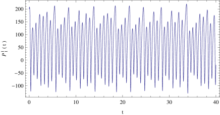
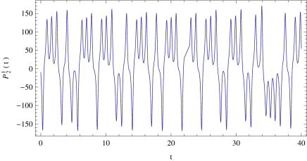
Figure 2: Time variation of the deviation curvature tensor component $P_{1}^{1}(t)$, shown in the left figure, and the time variation of $P_{2}^{1}(t)$, presented in the right figure, for $\sigma=10$, $\rho=28$, and $\beta=8/3$, respectively. The initial conditions used for the numerical integration of the Lorenz system are $X(0)=1$, $Y(0)=5$, and $Z(0)=10$.

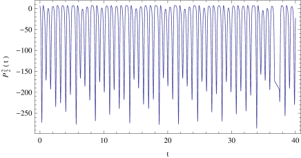
Figure 3: Time variation of the deviation curvature tensor component $P_{1}^{2}(t)$, presented in the left figure, and the time variation of $P_{2}^{2}(t)$, shown in the right figure, for $\sigma=10$, $\rho=28$, and $\beta=8/3$, respectively. The initial conditions used for the numerical integration of the Lorenz system are $X(0)=1$, $Y(0)=5$, and $Z(0)=10$.

The third, fourth and fifth KCC invariants, as defined by Eqs. (29) are identically equal to zero for the Lorenz system. However, the third invariant as defined by Eq. (30) has a non-zero component. Generally, the third KCC invariant can be written as

$$B_{jk}^{i}=\frac{\partial N_{j}^{i}}{\partial X^{k}}-\frac{\partial N_{k}^{i}}{\partial X^{j}}+N_{j}^{m}\frac{\partial N_{k}^{i}}{\partial Y^{m}}-N_{k}^{l}\frac{\partial N_{j}^{i}}{\partial Y^{l}},$$ (52)

which has a single non-zero component,

$$B_{12}^{2}=-N^{1}_{2}\frac{\partial N_{1}^{2}}{\partial Y^{1}}=-\frac{1+\sigma}{2\sigma}.$$ (53)

All the other KCC invariants of the Lorenz system are identically equal to zero.

IV.2 The Jacobi stability of the equilibrium points of the Lorenz system

The three equilibrium points of the Lorenz system are $S_{0}(0,0,0)$, if $\rho\leq 1$,
$S_{+}\left[\sqrt{\beta\left(\rho-1\right)},\sqrt{\beta\left(\rho-1\right)},\rho-1\right]$, and $S_{-}\left[-\sqrt{\beta\left(\rho-1\right)},-\sqrt{\beta\left(\rho-1\right)},\rho-1\right]$, if $\rho>1$, respectively. From the point of view of the second order differential formulation of the Lorenz system and of the Jacobi analysis, the equilibrium points of the system given by Eqs. (11) and (II.1) are

$$S_{0}\left(X^{1}_{0}=0,X^{2}_{0}=0\right),\rho\leq 1,$$ (54)

$$S_{+}\left[X^{1}_{+}=\sqrt{\beta(\rho-1)},X_{+}^{2}=\rho-1\right],\rho>1,$$ (55)

and

$$S_{-}\left[X^{1}_{-}=-\sqrt{\beta(\rho-1)},X_{-}^{2}=\rho-1\right],\rho>1,$$ (56)

respectively.

In the equilibrium points the components of the first KCC invariant vanish identically, so that

$$\epsilon^{i}\left(S_{0}\right)=\epsilon^{i}\left(S_{+}\right)=\epsilon^{i}\left(S_{-}\right)\equiv 0,i=1,2.$$ (57)

We evaluate now the components of the curvature deviation tensor in the equilibrium points. First we obtain

$$P_{1}^{1}\left(S_{0}\right)=-(1-\rho)\sigma+\frac{1}{4}\left(1+\sigma\right)^{2},\rho\leq 1$$ (58)

$$P_{1}^{2}\left(S_{0}\right)=P_{2}^{1}\left(S_{0}\right)=0,\rho\leq 1$$ (59)

$$P_{2}^{2}\left(S_{0}\right)=\beta^{2},\rho\leq 1,$$ (60)

For the equilibrium points $S_{+}$ and $S_{-}$ we obtain

$$P_{1}^{1}\left(S_{+}\right)=\frac{1}{4}(1+\sigma)^{2},\rho>1,$$ (61)

$$P_{2}^{1}\left(S_{+}\right)=-\sigma\sqrt{\beta(\rho-1)},\rho>1,$$ (62)

$$P_{1}^{2}\left(S_{+}\right)=\frac{\sqrt{\beta(\rho-1)}\left(-7\beta\sigma+\beta-\sigma^{2}+1\right)}{4\sigma},\rho>1,$$ (63)

$$P_{2}^{2}\left(S_{+}\right)=\beta^{2}-\beta\left(\rho-1\right),\rho>1,$$ (64)

and

$$P_{1}^{1}\left(S_{-}\right)=\frac{1}{4}(1+\sigma)^{2},\rho>1,$$ (65)

$$P^{1}_{2}\left(S_{-}\right)=\sigma\sqrt{\beta(\rho-1)},\rho>1,$$ (66)

$$P^{2}_{1}\left(S_{-}\right)=\frac{\sqrt{\beta(\rho-1)}\left(\beta(7\sigma-1)+\sigma^{2}-1\right)}{4\sigma},\rho>1,$$ (67)

$$P_{2}^{2}\left(S_{-}\right)=\beta^{2}-\beta\left(\rho-1\right),\rho>1,$$ (68)

respectively.

The eigenvalues of the curvature deviation tensor in the equilibrium points are obtained as

$$\lambda_{+}\left(S_{0}\right)=\frac{1}{4}\left[\sigma(4\rho+\sigma-2)+1\right],\lambda_{-}\left(S_{0}\right)=\beta^{2},\rho\leq 1,$$ (69)

$$\lambda_{+}\left(S_{+}\right) = \frac{1}{2}\Bigg{\{}\sqrt{\left[\beta\left(\beta-\rho+1\right)-\frac{1}{4}(\sigma+1)^{2}\right]^{2}+\beta(\rho-1)\left[\beta(7\sigma-1)+\sigma^{2}-1\right]}+$$ (70)

$$\beta(\beta-\rho+1)+\frac{1}{4}(\sigma+1)^{2}\Bigg{\}},\rho>1,$$

$$\lambda_{-}\left(S_{+}\right) = \frac{1}{2}\Bigg{\{}-\sqrt{\left[\beta\left(\beta-\rho+1\right)-\frac{1}{4}(\sigma+1)^{2}\right]^{2}+\beta(\rho-1)\left[\beta(7\sigma-1)+\sigma^{2}-1\right]}+$$ (71)

$$\beta\left(\beta-\rho+1\right))+\frac{(\sigma+1)^{2}}{4}\Bigg{\}},\rho>1,$$

$$\lambda_{+}\left(S_{-}\right) = \frac{1}{2}\Bigg{\{}\sqrt{\left[\beta\left(\beta-\rho+1\right)-\frac{1}{4}(\sigma+1)^{2}\right]^{2}+\beta(\rho-1)\left(\beta(7\sigma-1)+\sigma^{2}-1\right)}+$$ (72)

$$\beta(\beta-\rho+1)+\frac{1}{4}(\sigma+1)^{2}\Bigg{\}},\rho>1,$$

$$\lambda_{-}\left(S_{-}\right) = \frac{1}{2}\Bigg{\{}-\sqrt{\left[\beta\left(\beta-\rho+1\right)-\frac{1}{4}(\sigma+1)^{2}\right]^{2}+\beta(\rho-1)\left(\beta(7\sigma-1)+\sigma^{2}-1\right)}+$$ (73)

$$\beta(\beta-\rho+1)+\frac{1}{4}(\sigma+1)^{2}\Bigg{\}},\rho>1.$$

The eigenvalues of the deviation curvature tensor have the property

$$\lambda_{+}\left(S_{+}\right)=\lambda_{+}\left(S_{-}\right),\lambda_{-}\left(S_{+}\right)=\lambda_{-}\left(S_{-}\right).$$ (74)

The trace $\kappa$ of the deviation curvature tensor, as well as the anisotropy $\theta$ of the Lorenz system are obtained as

$$\kappa\left(S_{0}\right)=\frac{1}{2}\left\{\beta^{2}+\frac{1}{4}\left[\sigma(4\rho+\sigma-2)+1\right]\right\},$$ (75)

$$\theta\left(S_{0}\right)=\frac{1}{2}\left\{-\beta^{2}+\frac{1}{4}[\sigma(4\rho+\sigma-2)+1]\right\},$$ (76)

$$\kappa\left(S_{+}\right)=\kappa\left(S_{-}\right)=\frac{1}{8}\left[4\beta(\beta-\rho+1)+(\sigma+1)^{2}\right],$$ (77)

and

$$\theta\left(S_{+}\right)=\theta\left(S_{-}\right)=\frac{1}{2}\sqrt{\left[\beta\left(\beta-\rho+1\right)-\frac{1}{4}(\sigma+1)^{2}\right]^{2}+\beta(\rho-1)\left[\beta(7\sigma-1)+\sigma^{2}-1\right]},$$ (78)

respectively.

Taking into account the previous results we can formulate the following theorem, giving the Jacobi properties of the equilibrium points of the Lorenz system:

Theorem. a) The equilibrium point $S_{0}\left(0,0\right)$ of the Lorenz system is Jacobi unstable.

b) If the free parameters $\beta$, $\rho>1$, and $\sigma$ of the Lorenz system satisfy simultaneously the constraints

$$\beta\left(\beta-\rho+1\right)+\frac{1}{4}(\sigma+1)^{2}<0,$$ (79)

and

$$\frac{1}{4}\beta\left\{\beta\left[-7\rho\sigma+\rho+\sigma(\sigma+9)\right]-2\sigma(\rho-1)(\sigma+1)\right\}>0,$$ (80)

respectively, then the equilibrium points $S_{+}\left[\sqrt{\beta(\rho-1)},\rho-1\right]$ and $S_{+}\left[-\sqrt{\beta(\rho-1)},\rho-1\right]$ of the Lorenz system are Jacobi stable, and Jacobi unstable otherwise.

V The onset of chaos in the Lorenz system

The behavior of the deviation vector $\xi^{i}$, $i=1,2$, giving the behavior of the trajectories of a dynamical system near a fixed point $x^{i}\left(t_{0}\right)$ is described Eqs. (24) and (25). In the case of the Lorenz system these equations can be written generally as

$$\frac{d^{2}\xi^{1}(t)}{dt^{2}}+(\sigma+1)\frac{d\xi^{1}(t)}{dt}+\sigma\left[(1-\rho)+X_{2}\right]\xi^{1}(t)+ \sigma X_{1}\xi^{2}(t)=0,$$ (81)

and

$$\sigma\frac{d^{2}\xi^{2}(t)}{dt^{2}}+\left[\left(\beta-\sigma+1\right)X_{1}-2Y_{1}\right]\frac{d\xi^{1}(t)}{dt}+\left[2\sigma(\beta-\rho+X_{2}+1)X_{1}+(\beta-\sigma+1)Y_{1}\right]\xi^{1}(t)+$$

$$\sigma(X_{1}-\beta)(\beta+X_{1})\xi^{2}(t)=0,$$ (82)

respectively. The deviation vector is obtained from its components as

$$\xi(t)=\sqrt{\left[\xi^{1}(t)\right]^{2}+\left[\xi^{2}(t)\right]^{2}}.$$ (83)

In order to obtain a quantitative description of the onset of chaos in the Lorenz system, we introduce, in analogy with the Lyapounov exponent, the instability exponents $\delta_{i}$, $i=1,2$, and $\delta$, defined as

$$\delta_{i}(S)=\lim_{t\rightarrow\infty}\frac{1}{t}\ln\left[\frac{\xi^{i}(t)}{\xi_{i0}}\right],i=1,2.$$ (84)

and

$$\delta(S)=\lim_{t\rightarrow\infty}\frac{1}{t}\ln\left[\frac{\xi(t)}{\xi_{10}}\right].$$ (85)

In the following we investigate the behavior of the solutions of Eqs. (81) and (V) near the critical points of the Lorenz system.

V.1 Behavior of the deviation vector near $S_{0}(0,0)$

Near the equilibrium point $S_{0}(0,0)$ the deviation equations Eqs. (81) and (V) take the form

$$\frac{d^{2}\xi^{1}(t)}{dt^{2}}+(\sigma+1)\frac{d\xi^{1}(t)}{dt}+(1-\rho)\sigma\xi^{1}(t)=0,$$ (86)

and

$$\frac{d^{2}\xi^{2}(t)}{dt^{2}}-\beta^{2}\xi^{2}(t)=0,$$ (87)

respectively. In this case the deviation equation for the origin of the Lorenz system can be separated in two independent equations, with the general solutions given by

$$\frac{\xi^{1}(t)}{\xi_{10}}=\frac{e^{\frac{1}{2}\left(\sqrt{4\rho\sigma+\left(\sigma-1\right)^{2}}-\sigma-1\right)t}-e^{\frac{1}{2}\left(-\sqrt{4\rho\sigma+(\sigma-1)^{2}}-\sigma-1\right)t}}{\sqrt{4\rho\sigma+(\sigma-1)^{2}}},$$ (88)

and

$$\xi^{2}(t)=\frac{e^{-\beta t}\left(e^{2\beta t}-1\right)}{2\beta}\xi_{20},$$ (89)

where we have used the initial conditions $\xi^{1}(0)=0,\dot{\xi}^{1}(0)=\xi_{10}$, and $\xi^{2}(0)=0,\dot{\xi}^{2}(0)=\xi_{20}$, respectively. The time behavior of $\xi^{2}(t)$ is determined only by the coefficient $\beta$ of the Lorenz system. For the deviation vector we obtain

$$\xi(t) = \Bigg{[}\frac{\xi_{20}^{2}}{\xi_{10}^{2}}\frac{\sinh^{2}(\beta t)}{4\beta^{2}}+\frac{e^{-\left(\sqrt{4\rho\sigma+(\sigma-1)^{2}}+\sigma+1\right)t}\left(e^{\sqrt{4\rho\sigma+(\sigma-1)^{2}}t}-1\right)^{2}}{4\rho\sigma+(\sigma-1)^{2}}\Bigg{]}^{1/2}.$$ (90)

The time dependence of the deviation vectors $\xi^{1}$ and $\xi^{2}$ is represented, for different values of the parameters $\sigma$, $\rho$, and $\beta$, in Fig. 4.

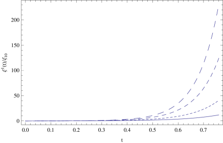
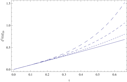
Figure 4: Time variation of the deviation vector components $\xi^{1}(t)/\xi_{10}$ (left figure) and $\xi^{2}(t)/\xi_{20}$ (right figure), in the vicinity of the equilibrium point $S_{0}$, for different values of the parameters $\beta$, $\rho$ and $\sigma$. In the left figure $\sigma=10$, $\beta=8/3$, and $\rho=15$ (solid curve), $\rho=20$ (dotted curve), $\rho=25$ (dashed curve), and $\rho=28$ (long dashed curve), respectively. In the right figure $\beta=2/3$ (solid curve), $\beta=5/3$ (dotted curve), $\beta=8/3$ (dashed curve), and $\beta=11/3$ (long dashed curve), respectively.

For a fixed $\beta$ and $\sigma$, with the increase of the parameter $\rho$, the deviation curvature component $\xi^{1}$ increases very rapidly in time, indicating the onset of chaos in the Lorenz system. In the large time limit the increase of $\xi^{1}(t)$ is exponential. The deviation curvature vector component $\xi^{2}$ also increases exponentially in time, a behavior that is independent of the values of $\beta$. The time variation of the absolute value of the deviation vector $\xi(t)$ is represented in Fig. 5.

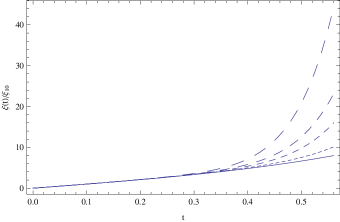
Figure 5: Time variation of the absolute value of the deviation vector $\xi(t)/\xi_{10}$ for $\beta=8/3$, $\sigma=10$, $\xi_{10}=10^{-9}$, $\xi_{20}=10^{-8}$, and for different values of $\rho$: $\rho=10$ (solid curve), $\rho=20$ (dotted curve), $\rho=25$ (dashed curve), $\rho=28$ (long dashed curve), and $\rho=33$ (ultra-long dashed curve, respectively.

With the increase of $\rho$ the absolute value of the deviation vector rapidly increases in time, indicating the onset of chaos in the Lorenz system. With the help of Eqs. (88) and (89) we immediately obtain

$$\delta_{1}\left(S_{0}\right)=\frac{1}{2}\left(\sqrt{4\rho\sigma+\left(\sigma-1\right)^{2}}-\sigma-1\right),$$ (91)

and

$$\delta_{2}\left(S_{0}\right)=\beta,$$ (92)

respectively. The instability exponent $\delta$ can be estimated as

$$\delta=\frac{1}{2t}\ln\left(\frac{\xi_{20}^{2}}{\xi_{10}^{2}}\frac{e^{2\beta t}}{4\beta^{2}}+\frac{e^{\sqrt{4\rho\sigma+(\sigma-1)^{2}}t}}{4\rho\sigma+(\sigma-1)^{2}}\right).$$ (93)

The time variation of the instability exponent $\delta$ is represented, for fixed values of the parameters $\beta$ and $\sigma$, in Fig. 6.

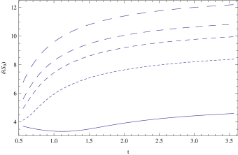
Figure 6: Time variation of the instability exponent $\delta$ for $\beta=8/3$, $\sigma=10$, $\xi_{10}=10^{-9}$, $\xi_{20}=10^{-8}$, and for different values of $\rho$: $\rho=10$ (solid curve), $\rho=20$ (dotted curve), $\rho=25$ (dashed curve), $\rho=28$ (long dashed curve), and $\rho=33$ (ultra-long dashed curve, respectively.

V.2 Dynamics of the deviation vector near $S_{+}\left[\sqrt{\beta(\rho-1)},\rho-1\right]$ and $S_{-}\left[-\sqrt{\beta(\rho-1)},\rho-1\right]$

For both fixed points $S_{+}\left[\sqrt{\beta(\rho-1)},\rho-1\right]$ and $S_{-}\left[-\sqrt{\beta(\rho-1)},\rho-1\right]$, the differential equations describing the dynamics of the deviation vector near the given fixed points take the form

$$\frac{d^{2}\xi^{1}(t)}{dt^{2}}+(\sigma+1)\frac{d\xi^{1}(t)}{dt}+\sigma\sqrt{\beta}\sqrt{\rho-1}\xi^{2}(t)=0,$$ (94)

and

$$\frac{d^{2}\xi^{2}(t)}{dt^{2}}+\frac{\sqrt{\beta}\sqrt{\rho-1}(\beta-\sigma+1)}{\sigma}\frac{d\xi^{1}(t)}{dt}+2\beta^{3/2}\sqrt{\rho-1}\xi^{1}(t)-\beta(\beta-\rho+1)\xi^{2}(t)=0,$$ (95)

respectively.

The behavior of the components of the deviation curvature vector is shown in Fig. 7.

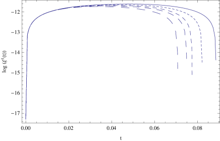
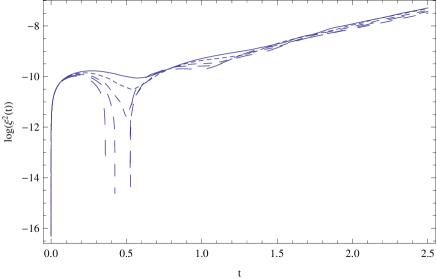
Figure 7: Time variation of the deviation vector components $\xi^{1}(t)$ (left figure) and $\xi^{2}(t)$ (right figure) in a logarithmic scale near the equilibrium points $S_{\pm}\left(\pm\sqrt{\beta(\rho-1)}\right)$, for $\beta=8/3$, $\sigma=10$, and for different values of $\rho$: $\rho=15$ (solid curve), $\rho=20$ (dotted curve), $\rho=25$ (dashed curve), $\rho=28$ (long dashed curve), and $\rho=33$ (ultra-long dashed curve, respectively. The initial conditions used to integrate the deviation equations are $\xi^{1}(0)=\xi^{2}(0)=0$, $\dot{\xi}^{1}(0)=10^{-10}$, and $\dot{\xi}^{2}(0)=10^{-9}$, respectively.

The time variation of the instability exponent $\delta\left(S_{+}\right)=\delta\left(S_{-}\right)$ is represented in Fig. 8.

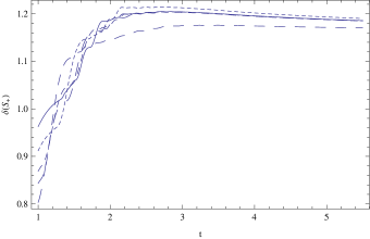
Figure 8: Time variation of the instability exponent $\delta\left(S_{+}\right)=\delta\left(S_{-}\right)$ near the equilibrium points $S_{\pm}\left(\pm\sqrt{\beta(\rho-1)}\right)$, for $\beta=8/3$, $\sigma=10$, and for different values of $\rho$: $\rho=15$ (solid curve), $\rho=20$ (dotted curve), $\rho=25$ (dashed curve), $\rho=28$ (long dashed curve), and $\rho=33$ (ultra-long dashed curve, respectively. The initial conditions used to integrate the deviation equations are $\xi^{1}(0)=\xi^{2}(0)=0$, $\dot{\xi}^{1}(0)=10^{-10}$, and $\dot{\xi}^{2}(0)=10^{-9}$, respectively.

V.3 The curvature of the deviation vector

In order to obtain a quantitative description of the behavior of the curvature deviation tensor in the following we analyze the signed geometric curvature $\kappa_{0}$ of the curve $\xi(t)=\left(\xi^{1}(t),\xi^{2}(t)\right)$, which we define, according to the standard approach used in the differential geometry of plane curves as

$$\kappa_{0}(S)=\kappa_{0}=\frac{\dot{\xi}^{1}(t)\ddot{\xi}^{2}(t)-\ddot{\xi}^{1}(t)\dot{\xi}^{2}(t)}{\left\{\left[\dot{\xi}^{1}(t\right]^{2}+\left[\dot{\xi}^{2}(t\right]^{2}\right\}^{3/2}}.$$ (96)

If we denote $\sqrt{4\rho\sigma+(\sigma-1)^{2}}=a$ and $\sigma+1=b$, we obtain an explicit formula for $\kappa_{0}$,

$$\kappa_{0} = \frac{\xi_{10}\xi_{20}}{8a}\frac{e^{(-b/2)t}}{\left\{\frac{\xi_{10}^{2}}{4a^{2}}[(a-b)e^{(a/2)t}+(a+b)e^{(-a/2)t}]^{2}e^{-bt}+\frac{\xi_{20}^{2}}{4}[e^{\beta t}+e^{-\beta t}]^{2}\right\}^{3/2}}\times$$ (97)

$$\Bigg{[}(a-b)(2\beta-a+b)e^{(a/2+\beta)t}+(a-b)(b-2\beta-a)e^{(a/2-\beta)t}+$$

$$(a+b)(2\beta+a+b)e^{(-a/2+\beta)t}+(a+b)(a+b-2\beta)e^{(-a/2-\beta)t}\Bigg{]}.$$

In the following we restrict our study to the equilibrium point $S_{0}(0,0)$, and we fix the values of the parameters as $\sigma=10$, $\beta=8/3$, $\xi_{10}=10^{-10}$, and $\xi_{20}=10^{-9}$, respectively. The variation of the curvature $\kappa_{0}$ is represented in Fig. 9.

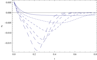
Figure 9: Time variation of the curvature $\kappa_{0}$ of the deviation vector $\xi(t)$ near the equilibrium points $S_{0}\left(0,0\right)$, for $\beta=8/3$, $\sigma=10$, $\dot{\xi}^{1}(0)=10^{-10}$, and $\dot{\xi}^{2}(0)=10^{-9}$, respectively, and for different values of $\rho$: $\rho=10$ (solid curve), $\rho=15$ (dotted curve), $\rho=20$ (dashed curve), $\rho=25$ (long dashed curve), $\rho=28$ (ultra-long dashed curve, and $\rho=33$ (ultra-ultra-long dashed curve), respectively.

As one can see from the figure, for the chosen range of the parameters the curvature of the two-dimensional deviation vector is positive for small values of time, reaches the value zero at a certain moment $t_{0}$, enters the region of the negative values, and then it tends to zero in the limit of large times. Near the time origin $t=0$ the curvature of the deviation vector curve can be represented in a form of a power series as

$$\kappa_{0}(t,\rho) \approx\frac{11}{202\sqrt{101}}-\frac{4545\sqrt{101}\rho+45584\sqrt{101}}{9272709}t+\frac{11\left(877185\sqrt{101}\rho+2748853\sqrt{101}\right)}{1873087218}t^{2}+...$$ (98)

In the first approximation the time interval $t_{0}$ for which $\kappa_{0}\left(t_{0},\rho\right)=0$ is given by

$$t_{0}\approx\frac{9999}{2(4545\rho+45584)}\approx\frac{1.099}{\rho+10.02}.$$ (99)

Therefore the time interval after which the curvature $\kappa_{0}$ changes sign is an indicator of the development of chaos in the Lorenz system. There exist therefore a critical time interval $t_{0}^{crit}$ so that if the transition from positive to negative $\kappa_{0}$ occurs at times $t>t_{0}^{crit}$, the evolution of the Lorenz system is predictable, and deterministic, while if the transition occurs for time intervals $t<t_{0}^{crit}$, then the underlying evolution of the Lorenz system will be chaotic in the long term. The curvature becomes zero when the two components of the deviation vector satisfy the condition $\xi^{1}\left(t_{0}\right)=\xi^{2}\left(t_{0}\right)$.

V.4 Comparing with linear stability analysis

We will now compare Jacobi stability and linear stability at the equilibrium point $S_{0}(0,0)$. The linearized Lorenz system at $(0,0,0)$ is given by

$$\left[\begin{array}[]{c}\dot{X}\\ \dot{Y}\\ \dot{Z}\\ \end{array}\right]=\left[\begin{array}[]{ccc}-\sigma&\sigma&0\\ \rho&-1&0\\ 0&0&-\beta\\ \end{array}\right]\left[\begin{array}[]{c}X\\ Y\\ Z\\ \end{array}\right].$$

We see that the equation for $Z$ is decoupled and $Z(t)$ tends to $0$ exponentially fast. The time dynamics of $X$ and $Y$ is governed by the two-dimensional system

$$\left[\begin{array}[]{c}\dot{X}\\ \dot{Y}\\ \end{array}\right]=\left[\begin{array}[]{cc}-\sigma&\sigma\\ \rho&-1\\ \end{array}\right]\left[\begin{array}[]{c}X\\ Y\\ \end{array}\right].$$

Let $A:=\left[\begin{array}[]{cc}-\sigma&\sigma\\ \rho&-1\\ \end{array}\right]$. Let $\tau=\mbox{trace}(A)$ and $\Delta=\det(A)$. Then,

$$\lambda_{1}=\frac{\tau+\sqrt{\tau^{2}-4\Delta}}{2},\quad\lambda_{2}=\frac{\tau-\sqrt{\tau^{2}-4\Delta}}{2}.$$

On the other hand, in Jacobi stability analysis, we find the eigenvalues of $P^{i}_{j}(0,0)$ are

$$\lambda_{+}\left(S_{0}\right) = \frac{1}{4}\left[\sigma(4\rho+\sigma-2)+1\right]=\frac{1}{4}(\tau^{2}-4\Delta),$$ (100)

$$\lambda_{-}\left(S_{0}\right) = \beta^{2},\rho\leq 1,$$ (101)

Thus, one of eigenvalues of $P^{i}_{j}(0,0)$ recovers some information of the stability of the system at the origin. That is, the origin is a center or spiral, when $\lambda_{+}\left(S_{0}\right)<0$.

VI Discussions and final remarks

In the present paper we have considered the stability analysis of the Lorenz system from the point of view of the KCC theory, in which the dynamical stability properties of dynamical systems are inferred from the study of the geometric properties of the Finsler space geodesic equations, equivalent with the given system. By transforming the Lorenz to an equivalent system of two second order differential equations, the dynamical system can be interpreted as representing the geodesic motion of a ”particle” in an associated Finsler space. This geometrization of the Lorenz system opens the possibility of applying the standard methods of differential geometry for the study of its properties. We have obtained, and analyzed in detail, the main geometrical objects that can be associated to the Lorenz system, namely, the non-linear connection, the Berwald connection, and the first, second and third KCC invariants. The main result of the present paper is the Jacobi stability condition of the equilibrium points of the Lorenz system, showing that the origin is always Jacobi unstable, while the Jacobi stability of the other two equilibrium points depends on the values of the parameters of the system. By considering the standard values of $\sigma$, $\beta$ and $\rho$ in the Lorenz system, $\sigma=10$, $\beta=8/3$, and $\rho=28$, it turns out that for this choice of the parameters all the equilibrium points are Jacobi unstable. From the point of view of linear stability analysis, for $0<\rho<1$, the zero fixed point $S_{0}=(0,0,)$ is globally stable; from a physical point of view this refers to the non convective state. For $\rho>l$ and $\rho$ not too large, the state with roll convection, referring to the $S_{\pm}$ equilibrium points, is stable And . From a physical point of view this means that the phase space consists of two regions, which are separated by the stable manifold of the zero fixed point; the trajectories which start in one of the two regions are attracted by the corresponding nonzero fixed point.

We have also considered in detail the behavior of the deviation vector near the equilibrium points. In order to describe the behavior of the trajectories near the equilibrium points we have introduced the instability exponent $\delta$, as well as the curvature $\kappa_{0}$ of the deviation vector trajectories. The curvature $\kappa_{0}$ of the curve $\xi(t)$ can be related directly to the chaotic behavior of the trajectories via its transition moment from positive to negative values. An early transition indicates the presence of chaotic states. Therefore we suggest the use of the curvature of the deviation vector as an indicator of the onset of chaos in non-linear dynamical systems. In T1 it was suggested that the torsion tensor geometrically expresses the chaotic behavior of dynamical systems, i.e. a trajectory of dynamical systems with the torsion tensor is not closed. By using the same definition as in T1 it turns out that indeed there is a non-zero torsion tensor component $B_{12}^{2}=-(1+\sigma)/2\sigma\neq 0$, $\forall\sigma\neq 0$. Therefore the existence of chaos in the Lorenz system is intimately related to a non-zero $\sigma$, which is needed for the chaotic behavior of the Lorenz system Pel .

References

- (1) A. M. Mancho, D. Small, and S. Wiggins, Physics Reports 437, 55 (2006).
- (2) G. Boffetta, M. Cencini, M. Falcioni, and A. Vulpiani, Physics Reports 356, 367 (2002).
- (3) A. E. Motter, M. Gruiz, G. Károlyi, and T. Tél, Phys. Rev. Lett. 111, 194101 (2013).
- (4) E. G. Altmann, J. S. E. Portela, and T. Tél, Phys. Rev. Lett. 111, 144101 (2013).
- (5) C. Skokos, I. Gkolias, and S. Flach, Phys. Rev. Lett. 111, 064101 (2013).
- (6) D. Pazó, J. M. López, and A. Politi, Phys. Rev. E 87, 062909 (2013).
- (7) B. Schalge, R. Blender, J. Wouters, K. Fraedrich, and F. Lunkeit, Phys. Rev. E 87, 052113 (2013).
- (8) S. Zeeb, T. Dahms, V. Flunkert, E. Schöll, I. Kanter, and W. Kinzel, Phys. Rev. E 87, 042910 (2013).
- (9) C. J. Yang, W. D. Zhu, and G. X. Ren, Communications in Nonlinear Science and Numerical Simulation 18, 3271 (2013).
- (10) H.-Liu Yang, G. Radons, and H. Kantz, Phys. Rev. Lett. 109, 244101 (2012).
- (11) A. Politi, F. Ginelli, S. Yanchuk, and Y. Maistrenko, Physica D: Nonlinear Phenomena 224, 90 (2006).
- (12) D. D. Kosambi, Math. Z. 37, 608 (1933).
- (13) E. Cartan, Math. Z. 37, 619 (1933).
- (14) S. S. Chern, Bulletin des Sciences Mathematiques 63, 206 (1939).
- (15) C. G. Boehmer, T. Harko, and S. V. Sabau, Adv. Theor. Math. Phys. 16 (2012) 1145-1196.
- (16) P. L. Antonelli (Editor), Handbook of Finsler geometry, vol. 1, Kluwer Academic, Dordrecht, (2003).
- (17) S. V. Sabau, Nonlinear Analysis 63, 143 (2005).
- (18) S. V. Sabau, Nonlinear Analysis: Real World Applications 6, 563 (2005).
- (19) P. L. Antonelli, Tensor, N. S. bf 52, 27 (1993).
- (20) T. Yajima and H. Nagahama, J. Phys. A: Math. Theor. 40, 2755 (2007).
- (21) T. Harko and V. S. Sabau, Phys. Rev. D 77, 104009 (2008).
- (22) C. G. Boehmer and T. Harko, Journal of Nonlinear Mathematical Physics 17, 503 (2010).
- (23) M. Pettini, Phys. Rev. E 47, 828 (1993).
- (24) H. E. Kandrup, Phys. Rev. E 56, 2722 (1997).
- (25) M. Di Bari, D. Boccaletti, P. Cipriani, and G. Pucacco, Phys. Rev. E 55, 6448 (1997).
- (26) P. Cipriani and M. Di Bari, Phys. Rev. Lett. 81, 5532 (1998).
- (27) M. Di Bari and P. Cipriani, Planet. Space. Science 46, 1543 (1998).
- (28) L. Casetti, M. Pettini, and E. G. D. Cohen, Physics Reports 337, 237 (2000).
- (29) G. Ciraolo and M. Pettini, Celestial Mechanics and Dynamical Astronomy 83, 171 (2002).
- (30) R. Punzi and M. N. R. Wohlfarth, Phys. Rev. E 79, 046606 (2009).
- (31) E. N. Lorenz, J. Atmos. Sci., 20, 130 (1963).
- (32) C. Sparrow, The Lorenz Equations: Bifurcations, Chaos, and Strange Attractors, Springer-Verlag, New York, (1982).
- (33) A. J. Lichtenberg, M. A. Lieberman, Regular and Chaotic Dynamics, 2nd ed., Springer-Verlag, New York, (1992).
- (34) R. Festa, A. Mazzino, and D. Vincenzi, Phys. Rev. E 65, 046205 (2002).
- (35) J. B. Gao, W.-W. Tung, and N. Rao, Phys. Rev. Lett. 89, 254101 (2002).
- (36) B.-L. Hao, J.-X. Liu, and W.-M. Zheng, Phys. Rev. E 57, 5378 (1998).
- (37) S. M. Zoldi, Phys. Rev. Lett. 81, 3375 (1998).
- (38) J. Alvarez-Ramírez, Phys. Rev. E 50, 2339 (1994).
- (39) V. Pelino and F. Maimone, Phys. Rev. E 76, 046214 (2007).
- (40) T. Yajima and H. Nagahama, Acta Mathematica Academiae Paedagogicae Nyíregyháziensis 24, 179 (2008).
- (41) T. Yajima and H. Nagahama, Physics Letters A 374, 1315 (2010).
- (42) O. E. Rössler, Phys. Lett. A 57, 397 (1976); O. E. Rössler, Phys. Lett A 60, 392 (1977).
- (43) R. Miron and C. Frigioiu, Algebras Groups Geom. 22, 151 (2005).
- (44) R. Miron, D. Hrimiuc, H. Shimada and V. S. Sabau, The Geometry of Hamilton and Lagrange Spaces, Kluwer Acad. Publ., Dordrecht; Boston (2001).
- (45) Q. I. Rahman and G. Schmeisser, Analytic theory of polynomials. London Mathematical Society Monographs. New Series 26. Oxford, Oxford University Press (2002).
- (46) R. F. S. Andrade and A. Rauh, Z. Phys. B - Condensed Matter 50, 151 (1983).