Magnetic response of a disordered binary ferromagnetic alloy to an oscillating magnetic field

Abstract

By means of Monte Carlo simulation with local spin update Metropolis algorithm, we have elucidated non-equilibrium phase transition properties and stationary-state treatment of a disordered binary ferromagnetic alloy of the type $A_{p}B_{1-p}$ on a square lattice. After a detailed analysis, we have found that the system shows many interesting and unusual thermal and magnetic behaviors, for instance, the locations of dynamic phase transition points change significantly depending upon amplitude and period of the external magnetic field as well as upon the active concentration of $A-$ type components. Much effort has also been dedicated to clarify the hysteresis tools, such as coercivity, dynamic loop area as well as dynamic correlations between time dependent magnetizations and external time dependent applied field as a functions of period and amplitude of field as well as active concentration of of $A-$ type components, and outstanding physical findings have been reported in order to better understand the dynamic process underlying present system.

1 Introduction

It was shown, for the first time, by theoretically that when a ferromagnetic material with coupling $J$ is exposed to a time dependent driving oscillating magnetic field, the system may not respond to the external magnetic field instantaneously, which gives rise to the existence of unusual and interesting behaviors due to the competing time scales of the relaxation behavior of the system and period of the external magnetic field [1]. A typical ferromagnet exists in dynamically disordered (P) phase where the time dependent magnetization oscillates around value of zero for the high temperature and amplitude of field regimes. At this stage, the time dependent magnetization of system is capable to follow the external field with relatively small phase lag. However, it oscillates around a non-zero value which indicates a dynamically ordered (F) phase for low temperatures and small amplitude of field regimes. After that, a great deal of studies concerning the non-equilibrium phase transitions and also hysteresis behaviors of different types of magnetic systems has been investigated by using both experimental and theoretical techniques. For the sake of completeness, it is beneficial to talk about some of the prominent experimental and theoretical studies, respectively. Actually, most of the experimental works have been devoted to the dynamic phase transitions and hysteretic treatments of different types of thin films [2, 3, 4, 5, 6, 7]. For example, in Ref. [5], dynamic magnetization reversal behavior of polycrystalline $\mathrm{Ni_{80}Fe_{20}}$ films has been studied by applying a magnetic field along the easy axis of the sample and it is found that the hysteresis loop area $A\left(=\oint MdH\right)$ is found to follow the scaling relation $A\propto H_{0}^{\alpha}\Omega^{\beta}T^{-\gamma}$ with $\alpha\approx 0.9$, $\beta\approx 0.8$ and $\gamma=0.38$, where $H_{0},\;\Omega$ and $T$ are the amplitude, frequency of the external magnetic field and temperature, respectively. Moreover, it has been shown recently by Berger et al. in Ref. [7] that uniaxial $\mathrm{Co}$ film sample under the influence of both bias (namely time independent) and time dependent oscillating magnetic fields in the vicinity of dynamic phase transition displays transient behavior for $\tau<\tau_{c}$, where $\tau$ and $\tau_{c}$ are period and critical period of the external applied field. Based on the experimental investigations we mentioned briefly above, it has been discovered that experimental non-equilibrium dynamics of considered real magnetic systems strongly resemble the dynamic behavior predicted from theoretical calculations of a kinetic Ising model.

On the other hand, from the theoretical point of view, dynamic phase transitions as well as hysteresis properties of both bulk and finite size lattice systems have been clarified within the frameworks of Mean-Field Theory (MFT) [8, 9, 10, 11, 12, 13], Effective-Field Theory (EFT) with single-site correlations [14, 15, 16, 17, 18, 19, 20, 21], as well as method of Monte Carlo (MC) simulations [21, 22, 23, 24, 25, 26, 27, 28, 29, 30, 31, 32, 33]. For example, by benefiting from a detailed large-scale MC simulation, in Ref. [30], Park and Pleimling considered kinetic Ising models with surfaces subjected to a periodic oscillating magnetic field to probe the role of surfaces at dynamic phase transitions. They reported that the non-equilibrium surface universality class differs from that of the equilibrium system, although the same universality class prevails for the corresponding bulk systems. Moreover, by making use of MC simulation with local spin update Metropolis scheme, dynamic phase transition features and stationary-state behavior of a ferrimagnetic nanoparticle system with core-shell structure have been recently analyzed by some of us in Ref. [31]. It has been observed that the particle may exhibit a phase transition from P to F phase with increasing ferromagnetic shell thickness in the presence of ultra-fast switching fields. Apart from these, there exists a limited number of theoretical studies about the non-equilibrium phase transition properties of magnetic systems containing quenched randomness resulting from random interactions between the spins with the same magnitudes or from a random dilution of the magnetic ions with non-magnetic species on the magnetic materials [18, 19, 34, 35, 36]. It is clear that these studies have a crucial role to have a better insight of the physics behind on real materials since a lot of magnetic materials have some small defects, and magnetic properties, i.e. phase transition temperature point of sample varies significantly depending on the type of defects.

In this letter, for the first time we intend to determine the magnetic phase transition and hysteretic properties of a disordered binary ferromagnetic alloy of the type $A_{p}B_{1-p}$ system under a magnetic field that oscillates in time. Such a quenched disordered system consists of two different species of magnetic components, namely $A$ and $B$, and we select the magnetic components $A$ and $B$ to be as $S_{A}=1/2$ and $S_{B}=1$, respectively. Here, $p$ refers to the concentration of type-$A$ magnetic ion. The square lattice sites are randomly occupied by $A$ and $B$ atoms depending on the selected concentrations of magnetic components. Before going further, we should note that equilibrium or static features of such of disordered binary magnetic systems have been analyzed by means of several types of frameworks such as Perturbation Theory [37], MFT [37, 38, 39, 40], Bethe-Peirls Approximation [41], EFT with single-site correlations [42, 43, 44, 45, 46, 47, 48] and method of MC simulation [49, 50, 51, 52, 53]. For instance, the critical properties of random mixtures of ferromagnetic and anti-ferromagnetic spin-spin interactions have been studied with MC simulation on a simple cubic lattice in Ref. [49]. It has been found that the system exhibits spin-glass phase characterized by a cusp-like peak in the susceptibility. Additionally, it is claimed by the author in Ref. [39] that random-site binary ferromagnetic Ising model shows seven topologically different types of phase diagrams including a variety of multi-critical points within the framework MFT.

The main motivation of the present study is to look answers for the physical facts underlying below questions:

• What is the effect of the amplitude and frequency of the external magnetic field on the dynamic phase transition properties (i.e. critical temperature) of the considered system?

• What kind of physical relationships exist between the magnetic properties (i.e. dynamic loop area, dynamic correlation and coercivity) of the system and the concentration of $A$-type magnetic components? In other words, whether the macroscopic treatments of the observable quantities of system depend on the concentration of $A$-type magnetic components or not.

The plan of the remainder parts of the paper is as follows: In section (2) we briefly present our model. The results and discussions are presented in section (3), and finally section (4) contains our conclusions.

2 Formulation

The system simulated here, which is schematically shown in Fig. 1, is a disordered binary ferromagnetic alloy of the type $A_{p}B_{1-p}$ which is defined on a two dimensional regular square lattice under the existence of a time dependent driving oscillating magnetic field. The lattice sites are randomly occupied by two different species of magnetic components $A$ and $B$ with the concentration $p$ and $1-p$, respectively. Thus, the Hamiltonian of the considered system can be written in the following form:

$$\hat{H}=-J\sum_{\langle i,j\rangle}\left[\delta_{i}\delta_{j}\sigma_{i}\sigma_{j}+(1-\delta_{i})(1-\delta_{j})S_{i}S_{j}+\delta_{i}(1-\delta_{j})\sigma_{i}S_{j}+(1-\delta_{i})\delta_{j}S_{i}\sigma_{j}\right]-H(t)\sum_{i}\left(\delta_{i}\sigma_{i}+(1-\delta_{i})S_{i}\right),$$ (1)

where $J>0$ is the ferromagnetic exchange interaction energy between $i$ and $j$ sites. The $\sigma$ and $S$ are conventional Ising spin variables which can take values of $\sigma=\pm 1/2$ and $S=\pm 1,0$ for the magnetic $A$- and $B$- components of system, respectively. $\delta_{i}$ is a random variable which can take value of unity or zero depending on whether the site-$i$ is occupied by $A$ or $B$ ion, respectively. The first summation in Eq. (1) is over the nearest-neighbor pairs while the second one is over all lattice sites in the system. $H(t)$ denotes the time dependent oscillating magnetic field described as $H(t)=h_{0}sin(\omega t)$, where $t$ is time, $h_{0}$ and $\omega$ are amplitude and angular frequency of the driving magnetic field, respectively. The period of the oscillating magnetic field is given by $\tau=2\pi/\omega$.

Figure 1: Schematic representation of the system of the type $A_{p}B_{1-p}$ for five selected active concentration values of $A$-type magnetic component, namely (a) $p=0.0$, (b) $p=0.25$, (c) $p=0.5$, (d) $p=0.75$ and (e) $p=1.0$. The blue and red colors correspond to $A$ and $B$ types of magnetic components which are randomly distributed.

We simulate the system specified by the Hamiltonian in Eq. (1) on a $L\times L$, where $L=128$, square lattice under periodic boundary conditions applied in all directions by benefiting from MC simulation with single-spin flip Metropolis algorithm [54, 55]. The general simulation procedure we use in this study is as follows: The simulation begins from high temperature using random initial conditions, and then the system is slowly cooled down with the reduced temperature steps $k_{B}\Delta T/J=0.015$, where configurations were generated by selecting the sites randomly through the lattice and making single-spin-flip attempts, which were accepted or rejected according to the Metropolis algorithm. The numerical data were generated over 50 independent sample realizations by running the simulations for 20000 MC steps per site after discarding the first 10000 steps. This amount of transient steps is found to be sufficient for thermalization for the whole range of the parameter sets.

Our program calculates the instantaneous values of the magnetizations $M_{A}(t)$ and $M_{B}(t)$, and also the total magnetization $M_{T}(t)$ at time $t$ as follows:

$$M_{A}(t)=\frac{1}{L^{2}}\sum_{i=1}^{N_{A}}\sigma_{i},\quad\quad\quad M_{B}(t)=\frac{1}{L^{2}}\sum_{i=1}^{N_{B}}S_{i},\quad\quad\quad M_{T}(t)=M_{A}(t)+M_{B}(t),$$ (2)

where $N_{A}$ denotes the total number of $A$ ions ($N_{A}=pL^{2}$) while $N_{B}$ represents the total number of $B$ ions ($N_{B}=(1-p)L^{2}$). Further, utilizing the instantaneous magnetizations stated in Eq. (2), we determine the dynamic loop area which measures the energy loss of the system due to the hysteresis, and dynamic correlations between time dependent magnetic field and magnetizations, respectively as follows [28]:

$$A_{\alpha}=-\oint M_{\alpha}(t)dH,\quad\quad\quad C_{\alpha}=\frac{1}{\tau}\oint M_{\alpha}(t)H(t)dt,$$ (3)

here $\alpha=A,B$ and $T$. Namely, $A_{A},A_{B}$, and $A_{T}$ correspond to the dynamic loop areas while $C_{A},C_{B}$, and $C_{T}$ refer to the dynamic correlations of magnetic components $A$, $B$ and total system, respectively.

In order to specify the location of dynamic phase transition point at which F and P phases separate from each other, we use and check the thermal variation of dynamic heat capacity and which is defined as:

$$C=\frac{dE_{Coop}}{dT},$$ (4)

where $T$ is temperature while $E_{Coop}$ is the cooperative part of the energy over a full cycle of the external applied magnetic field which is defined according to the following equation:

$$E_{Coop}=-\frac{1}{\tau L^{2}}\oint\left[J\sum_{\langle i,j\rangle}\left[\delta_{i}\delta_{j}\sigma_{i}\sigma_{j}+(1-\delta_{i})(1-\delta_{j})S_{i}S_{j}+\delta_{i}(1-\delta_{j})\sigma_{i}S_{j}+(1-\delta_{i})\delta_{j}S_{i}\sigma_{j}\right]\right]dt.$$ (5)

3 Results and Discussion

In this section, in order to explain the dynamic evolution of the magnetic system in detail, we will focus our attention on non-equilibrium phase transition properties as well as stationary-state treatment of the quenched disordered binary ferromagnetic alloy system under a time dependent oscillating magnetic field. We argue and discuss how the amplitude and period of the external oscillating magnetic field as well as concentration of $A$-type magnetic component affect the dynamic critical nature of the system. We will also shed light on the physical facts lying behind the thermal dependencies of dynamic loop areas as well as correlations between time dependent magnetizations and magnetic field for some selected combination of system parameters. As a final investigation, we examine the variations of coercivity and also hysteresis behavior as functions of system parameters, as well as active concentration of $A$-type magnetic component.

Before going further, it should be emphasized that for $h_{0}/J=0.0$, i.e. static case, our numeric MC simulation findings are completely in accordance with the recently published work [53] where thermal equilibrium phase transition properties of the system we consider have been addressed by utilizing MC simulation with Metropolis algorithm. Let us start to discuss the non-equilibrium phase transition properties of the system. In Figs. 2(a-c), we give the global dynamic phase boundaries that distinguish between F and P phases in a ($p-k_{B}T_{c}/J$) space with five reduced external field amplitude values, such as $h_{0}/J=0.0,0.25,0.5,0.75$ and $1.0$ for some considered values of oscillation periods, namely $\tau=50,100$ and $200$. At first sight, one can easily see from the figure that, $(i)$ for a fixed set of values of $h_{0}/J$ and $\tau$, when the concentration of spin-$1/2$ atom is increased starting from $p=0.0$ [56], F to P phase transition point moves to a lower value in temperature axis. This is because of the fact that the system tends to become disordered due to the occurrence of two different types of randomly occupied magnetic components as the active concentration of spin-$1/2$ is increased starting from $p=0.0$.

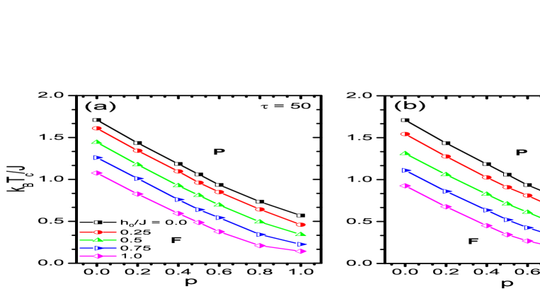
Figure 2: Dynamic phase diagrams in $(p-k_{B}T_{C}/J)$ planes obtained from the peaks of the dynamic heat capacity for values of $h_{0}/J=0.0,0.25,0.5,0.75$ and 1.0. The curves are demonstrated for three values of oscillation periods: (a) $\tau=50$, (b) $\tau=100$ and (c) $\tau=200$. The characters F and P refer to the dynamically ferromagnetic and paramagnetic phases, respectively.

It is possible to say that as the $p$ value is increased then the energy contribution which comes from spin-spin interactions gets smaller. Consequently, the F to P phase transition point moves to a lower temperature, due to the energy resulting from the temperature and (or) magnetic field which overcome the ferromagnetic spin-spin interactions. Therefore, the F regions in $(p-k_{B}T_{C}/J)$ plane get narrower. Moreover, $(ii)$ for a fixed set of values of $p$ and $\tau$, we see that when $h_{0}/J$ increases, then the magnetic energy supplied by the external applied field dominates against the ferromagnetic spin-spin exchange interactions, and hereby, the studied system can relax within the oscillation period $\tau$ of the external field which gives rise to a reduction in the transition temperature. In order to see this physical fact, one can compare any two values of applied field amplitudes, for example $h_{0}/J=0.25$ with 0.5 for $p=0.8$ in Fig.2(a). Another important finding of our numerical simulation is that the location of the phase transition temperature sensitively depends on the applied field period. $(iii)$ For a fixed set of values $p$ and $h_{0}/J$, it is obvious that as $\tau$ is increased, the phase transition point is lowered since decreasing field frequency gives rise to a decreasing phase delay between the magnetizations and magnetic field (i.e. the magnetizations can follow the oscillating driving magnetic field) and this makes the occurrence of the dynamic phase transition easy. The physical discussions mentioned above can be easily seen by checking any two values of oscillation periods such as $\tau=100$ and $200$ for fixed values of $h_{0}/J=0.5$ and $p=0.8$.

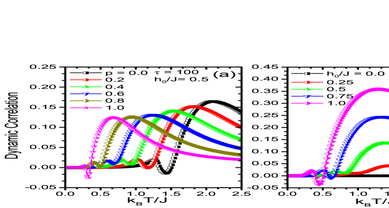
Figure 3: Thermal variations of dynamic total correlations corresponding to the dynamic phase diagrams shown in Figs. 2(a-c). The parameters we study are remarked on the graphs.

We draw in Figs. 3(a-c) the active concentration of $A$-type magnetic component, reduced amplitude and oscillation period of field dependencies of dynamic correlation versus temperature curves. One can able to deduce from the figures that, at relatively low temperature regions where the system exists in F phase, the dynamic correlations between time dependent magnetizations of the system and forcing field are close to zero since thermal energy is almost negligible, and the ferromagnetic spin-spin interactions are dominant against the field energy. Moreover, the system begins to show a shallow dip behavior, which may become negative depending on the system parameters, in the vicinity of dynamic phase transition point of system. For example, the dynamic correlation curves exhibit concentration, reduced amplitude and oscillating period of field induced negative shallow dip behavior in Figs. 3(a), (b) and (c), respectively.

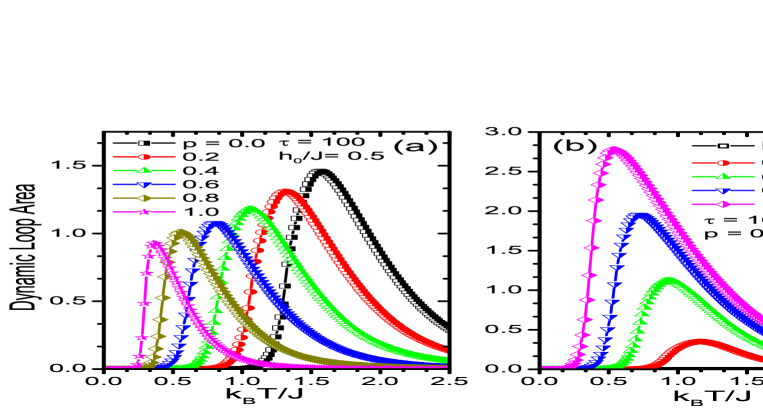
Figure 4: Temperature variations of dynamic total loop areas for varying system parameters which are indicated in related graphs.

In the following analysis, in order to show what happens in dynamic loop area versus temperature curves at varying system parameters, we give in Figs. 4(a-c) thermal variations of dynamic loop areas corresponding to the dynamic phase diagrams illustrated in Figs. 2(a-c). As indicated in section (2), dynamic loop area characterizes energy dissipation due to the hysteresis. It can be readily seen from the figures that the dynamic loop area curves obtained for a wide range of system parameters reveal a smooth and rounded cusp located at a certain temperature above the dynamic phase transition temperature of system. It would be interesting to see the origin of the physical mechanisms underlying on the thermal treatment of dynamic loop areas. Keeping this in mind, we separated the temperature space into five stages which are shown in Fig. 5 where dynamic loop areas of two different parts as well as of overall system have been plotted for selected values of system parameters such as $p=0.5,\;h_{0}/J=0.5$ and $\tau=100$. At stage-I, the temperature is sufficiently low so that both magnetic components $A$ and $B$ of the system show a dynamic ferromagnetism. In other words, the time dependent magnetizations of the system can not follow the external field simultaneously. Hence, dynamic loop areas of the system are close to zero. If we look at stage-II, where the location of the stage-II corresponds to the dynamic critical temperature of the system for the parameters we select, we can see that an increment in temperature gives rise to a reduction of ferromagnetism, and time dependent magnetizations of the system begin to relatively respond to the time dependent external magnetic field. As a result of this, hysteresis loop areas of both magnetic components $A$ and $B$ of the system get wider. Before going further, we note that even though the stage-II is a phase transition point, the dynamic loop areas does not show a maximum peak at the position of stage-II. This is because of such MC computer experiments include of thermal fluctuations of spins. If one considers the same problem with MFT (or EFT) which neglects (or partially includes) the thermal fluctuations of spins, and focuses on the thermal evolution of dynamic loop areas of the system, with a high probability, one can see that thermal variation of dynamic loop area may exhibit a maximum at the dynamic phase transition point [19, 28]. Let us continue with stage-III where the dynamic loop areas of the system present a maximum peak, both magnetic components $A$ and $B$ of the system show a dynamic paramagnetism, i.e., the time dependent magnetizations of the system can follow the external field with a relatively small phase lag. As the temperature is increased above the dynamic transition point, we reach the stages-IV and -V, where the value of dynamic loop areas begin to reduce, respectively. Apart from the changing values of the dynamic loop area corresponding to different stages we determine, shapes of hysteresis curves sensitively depend on the selected system parameters which will be discussed below.

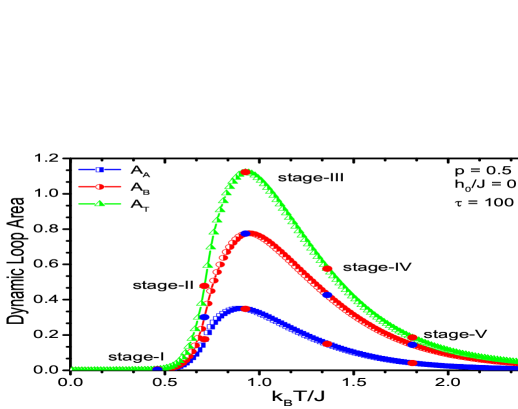
Figure 5: Thermal variations of dynamic loop areas of magnetic components $A$, $B$ and overall system for considered values of system parameters, such as $p=0.5,h_{0}/J=0.5$ and $\tau=100$. The labeled stage-$i$ ($i=$I, II,..,V) refers to the five different temperature locations indicated in graph.

In order to understand the varying temperature influences on the hysteresis treatments of the system, we give in Fig. 6 the hysteresis curves for both magnetic components $A$, $B$ and overall of the system for selected system parameters corresponding to the diagram depicted in Fig. 5. When we look at the hysteresis curves obtained for stage-I, we see that hysteresis loops are asymmetric around zero value indicating an F phase. If one moves throughout stage-I $\rightarrow$ stage-II way, it can be easily seen that the asymmetric shapes of hysteresis curves begin to slowly break down owing to the existence of a higher thermal energy than before. When the studied system attains the stage-III, it is possible to observe an example of square-like shape of hysteresis curves. In this zone, the system completely exhibits a P character. As the temperature increased, we reach the stage-IV, and we see that shape of hysteresis loops begin to change from square-like to sigmoidal-like shaped due to the thermal agitations. In addition to these, further increment in temperature leads to the occurrence of a narrower sigmoidal-like hysteresis curves which are explicitly shown in stage-V of figure. Similar of observations have been recently found in ultrathin Blume-Capel films under a magnetic field which oscillates in time [57].

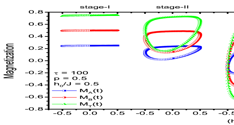
Figure 6: Hysteresis curve evolutions of both magnetic components $A$ and $B$ and also overall of system at different five temperature locations for the same system parameters with figure 5.

In the following two analysis, namely in Figs. 7 and 8, we investigate the oscillation period, reduced amplitude of external applied field and concentration of $A$-type magnetic component dependencies of the coercivity as well as hysteresis curves of the system. The aforementioned physical quantities have been calculated at a temperature $T=0.8T_{c}^{0}(p)$, where $T_{c}^{0}(p)$ is the static phase transition point in the absence of the external field, and it depends on the studied active concentrations of magnetic atoms. The reason why we choose such a temperature is that the system can be capable of undergoing a purely mechanical phase transition, such as applied field period or reduced amplitude induced phase transition. The numerical data were collected for 100 cycles of the external field after discarding the first 100 cycles of field have been discarded to obtain a stationary state behavior.

We give the period of external field dependencies of the coercivity of the system in Fig. (7) with varying values of reduced applied field amplitudes, such as $h_{0}/J=0.25,0.5,1.0,2.0$ and $4.0$ with three considered values of active concentration of $A$-type magnetic component, namely $p=0.0$, $0.5$ and $1.0$. It can be said by focusing on Fig. 7(a) that depending on the reduced applied field amplitude, it is possible to observe a large coercive field at low applied field periods. Moreover, it is found that coercivity curves of system exhibit a sudden variation with increasing applied field period whereas for sufficiently high $\tau$ they exhibit a stable profile. Another important point we want to emphasize is that the system has no coercivity value in the case of low values of applied field period and reduced amplitude, for example $\tau=100$ and $h_{0}/J=0.25$. In this regime, the system exists in F phase. However, with a significant increment in value of amplitude for the same period of field causes the existence of a purely mechanical reduced amplitude induced phase transition, and coercivity treatment begins to show itself naturally. The nearly same discussions are also valid for Figs 7(b-c) which are plotted for $p=0.5$ and $p=1.0$, respectively. As the type-$A$ magnetic component is introduced into the lattice, the coercivity value decreases prominently since the energy originating from the time dependent forcing field overcomes the ferromagnetic spin-spin interaction term between spin pairs in the lattice. Moreover, we should note that at the relatively low values of the amplitude and the period of the external field, even though some small number of spin flip occurs, the considered alloy system shows a dynamic ferromagnetic character. The physics mentioned briefly here is valid for all concentration values of the system.

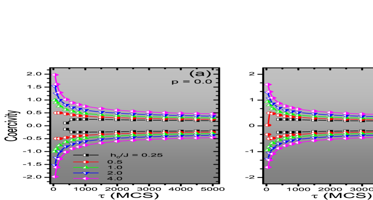
Figure 7: Variations of the coercive fields as a function of the oscillation period for several values of $h_{0}/J$ with (a) $p=0.0$, (b) $p=0.5$ and (c) $p=1.0$, respectively.

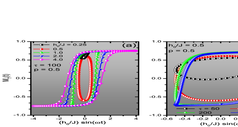
Figure 8: Influences of (a) reduced amplitudes for $\tau=100$, (b) relatively low periods, and (c) high periods of field for $h_{0}/J=0.5$ on the hysteresis loops of the system corresponding to the figure 7(b).

As a final investigation, we present the evolution of some typical hysteresis curves corresponding to the coercivity properties illustrated in Fig. 7. Throughout Figs. 8(a-c), we fix the active concentration of magnetic components as $p=0.5$ and change the external field components, namely period and reduced amplitude of field. In Fig. 8(a), we select the period of field as $\tau=100$ to investigate the influences of varying reduced amplitudes of field on hysteresis curves. It is clear from the figure that while the system exists in dynamically ordered phase and hysteresis curve is asymmetric around zero value at the relatively low reduced external field amplitude, i.e. $h_{0}/J=0.25$, with increasing amount of $h_{0}/J$ the system starts to show a dynamically paramagnetic character, and hysteresis curve is symmetric around zero value. According to our numerical findings, another important observation is that the shape of the hysteresis curves sensitively depend on the applied field amplitude, for example, while the hysteresis loop is broad square-like shaped for value of $h_{0}/J=0.5$, it is sigmoidal-like shaped for values of $h_{0}/J=1.0$, $2.0$ and $4.0$. In Fig. 8(b), we give the dynamic hysteresis loops obtained for selected values of applied field period such as $\tau=50,100,200$ and $400$ with fixed value of $h_{0}/J=0.5$. At first glance, by comparing the curves obtained for $\tau=50$ and $100$, one can clearly deduce from the figures that (i) remanent magnetization and also coercivity values of the system tend to change, (ii) the hysteresis curves begin to widen indicating a period of field induced phase transition with increasing $\tau$. If we increase $\tau$, the hysteresis curves becomes broad square-like shaped. On the other hand, in Fig. 8(c), it is possible to see that the hysteresis curves are sigmoidal shaped, and the width of the loops becomes narrower but does not vanish at the relatively high values of applied field period regimes. This type of behavior has been reported in [31, 32] where non-equilibrium phase transition properties of a nanocube system is investigated with MC method of simulation.

4 Conclusion

In conclusion, by making use of MC computer experiment method with Metropolis algorithm, we have looked for answers for the questions discussed in section 1. As we mentioned above, as a disordered binary ferromagnetic alloy with coupling $J$, we have selected a system consisting of spin-$1/2$ and spin-$1$ components, where the spin-$1/2$ and spin-$1$ components are distributed randomly depending upon the controllable concentration value. The situations of $p=1.0$ and $0.0$ correspond to the completely pure kinetic Ising and Blume-Capel models without single-ion anisotropy, respectively. Namely, for both two values of $p$ we remark, there is no lattice including disorder originating from different species of components in the system. However, it is obvious that except from these two values of $p$, the magnetic system composes of randomly distributed spin-$1/2$ and spin-$1$ components where the weights of the components strongly depend on the concentration values. After detailed numerical operations, the most prominent findings underlined in the present paper can be briefly summarized as follows:

• For a fixed set of values of $h_{0}/J$ and $\tau$, we found an almost linear decrease the critical temperature with increasing type-$A$ content.

• We see that when $h_{0}/J$ increases, then the magnetic energy supplied by the external applied field dominates against the ferromagnetic spin-spin exchange interactions, and hereby, the studied system can relax within the oscillation period $\tau$ of the external field which gives rise to a reduction in the transition temperature, for a fixed set of values $p$ and $\tau$.

• For a fixed set of values $p$ and $h_{0}/J$, as $\tau$ is increased, the phase transition point is lowered because of increasing field frequency gives rise to a growing phase delay between the time dependent magnetizations and forcing applied field.

The situations corresponding to the explanations we emphasize above can be easily seen by looking the dynamic phase boundaries separating the F and P phases which have been constructed in active concentration of spin-1/2 atoms and dynamic critical temperature planes at various Hamiltonian parameters in Fig. 1. Our simulation results also suggest that:

• For studied values of system parameters, thermal variations of dynamic correlations exhibit period and reduced amplitude of field as well as active concentration of $A$-type magnetic component induced local dip behavior.

• The locations of maximum lossy points which are characterized by hysteresis loop area show a decreasing tendency in temperature value with increasing $p$ values starting from zero for considered values of Hamiltonian parameters. Other system parameter dependencies of dynamic loop area has also been discussed in the present study.

• Applied field period dependencies of the coercivities obtained for three concentration values of $p$ with varying reduced amplitudes of field reveal that they exhibit a stable profile at the relatively high period of field whereas they show a sudden change in the low period of field. It is also found that for a fixed set of $h_{0}/J$ and $\tau$, as the $p$ value increases starting from zero, the corresponding coercivity value begins to decrease this is because of the amount of spin-1/2 atoms increases in system.

• Shape of the hysteresis curve of the system strongly depends on the taking Hamiltonian parameters into consideration. For example, while it is possible to observe an example of a broad square-like shaped hysteresis curve at the relatively low period of field, the shape of it begins to change to be a sigmoidal-like shape with increasing period of field.

All of the observations found in this work show that the amplitude and frequency of the driving time dependent magnetic field as well as active concentration of $A$-type magnetic component have an important influence on the thermal and magnetic properties, such as coercivity and critical temperature of the system.

Finally, we note that such a binary alloy system can actually contain four different values of relative $A-B$ interaction energy, namely $J_{AA}$, $J_{BB}$, $J_{AB}$, $J_{BA}$ corresponding to the randomly distributed components between $A-A$, $B-B$, $A-B$ and $B-A$, respectively. According to the findings of the previously published equilibrium phase transition studies mentioned in section 1, disordered binary alloy system with different signs and unequal magnitudes of the spin-spin interactions and single ion-anisotropy reveals interesting thermal and magnetic behaviors such as existence of re-entrant, compensation and also spin-glass behaviors. In this work, we have focused on only the non-equilibrium phase transition properties of disordered binary alloy system in cases of $J_{AA}=J_{BB}=J_{AB}=J_{BA}=J$ and also zero single-ion anisotropy. So, determination of the non-equilibrium phase transitions features of a disordered binary alloy including different types of spin-spin interactions and also single-ion anisotropy may be an interesting study. Furthermore, based on the earlier systems [10, 19, 35], it is possible to categorize the frequency dispersions of dynamic loop areas into three distinct types depending on the system parameters. Keeping in this mind, it would also be very interesting to see the frequency dispersions of dynamic loop areas of the same system.

5 Acknowledgements

The numerical calculations reported in this paper were performed at TÜBİTAK ULAKBİM (Turkish agency), High Performance and Grid Computing Center (TRUBA Resources).

References

- [1] T. Tomé, M.J. de Oliveira, Phys. Rev. A 41 (1990) 4251.
- [2] J.-S. Suen, J.L. Erskine, Phys. Rev. Lett. 78 (1997) 3567.
- [3] Y.-L He, G.-C. Wang, Phys. Rev. Lett. 70 (1993) 2336.
- [4] Q. Jiang, H.-N. Yang, G.-C. Wang, Phys. Rev. B 52 (1995) 14911.
- [5] B.C. Choi, W.Y. Lee, A. Samad, J.A.C. Bland, Phys. Rev. B 60 (1999) 11906.
- [6] D.T. Robb, Y.H. Xu, O. Hellwig, J. McCord, A. Berger, M.A. Novotny, P.A. Rikvold, Phys. Rev. B 78 (2008) 134422.
- [7] A. Berger, O. Idigoras, P. Vavassori, Phys. Rev. Lett. 111 (2013) 190602.
- [8] M. Acharyya, Phys. A 253 (1998) 199.
- [9] G.M. Buendía, M. Machado, Phys. Rev. E 58 (1998) 1260.
- [10] A. Punya, R. Yimnirun, P. Laoratanakul, Y. Laosiritaworn, Physica B 405 (2010) 3482.
- [11] M. Keskin, O. Canko, U. Temizer, Phys. Rev. B 72 (2005) 036125.
- [12] M. Keskin, E. Kantar, O. Canko, Phys. Rev. E 77 (2008) 051130.
- [13] O. Idigoras, P. Vavassori, A. Berger, Physica B 407 (2012) 1377.
- [14] X. Shi, G. Wei, L. Li, Phys. Lett. A 372 (2008) 5922.
- [15] X. Shi, J. Zhao, X. Xu, Physica A, 419 (2015) 234.
- [16] Y. Yuksel, E. Vatansever, U. Akinci, H. Polat, Phys. Rev. E 85 (2012) 051123.
- [17] U. Akinci, Y. Yuksel, E. Vatansever, H. Polat, Physica A 391 (2012) 5810.
- [18] E. Vatansever, B.O. Aktas, Y. Yuksel, U. Akinci, H. Polat, J. Stat. Phys. 147 (2012) 1068.
- [19] E. Vatansever, U. Akinci, Y. Yuksel, H. Polat, J. Magn. Magn. Mater. 329 (2013) 14.
- [20] B.O. Aktas, U. Akinci, H. Polat, Phys. Rev. E 90 (2014) 012129.
- [21] X. Shi, G. Wei, Phys. Scr. 89 (2014) 075805.
- [22] W.S. Lo, R.A. Pelcovits, Phys. Rev. A 42 (1990) 7471.
- [23] A. Chatterjee, B.K. Chakrabarti, Phys. Rev. E 67 (2003) 046113.
- [24] H. Park, M. Pleimling, Phys. Rev. E 87 (2013) 032145.
- [25] M. Acharyya, B.K. Chakrabarti, Phys. Rev. B 52 (1995) 6550.
- [26] M. Acharyya, J. Magn. Magn. Mater. 323 (2011) 2872.
- [27] M. Acharyya, Phys. Rev. E 69 (2004) 027105.
- [28] M. Acharyya, Phys. Rev. E 58 (1998) 179.
- [29] K. Tauscher, M. Pleimling, Phys. Rev. E 89 (2014) 022121.
- [30] H. Park, M. Pleimling, Phys. Rev. Lett. 109 (2012) 175703.
- [31] Y. Yuksel, E. Vatansever, H. Polat, J. Phys.: Condens. Matter 24 (2012) 436004.
- [32] E. Vatansever, H. Polat, Physica A 394 (2014) 82.
- [33] E. Vatansever, H. Polat, arXiv:1311.3537v2.
- [34] G.-P. Zheng, M. Li, Phys. Rev. B 66 (2002) 054406.
- [35] B.O. Aktas, U. Akinci, H. Polat, Physica B 407 (2012) 4721.
- [36] E. Vatansever, U. Akinci, H. Polat, J. Magn. Magn. Mater. 344 (2013) 89.
- [37] M.F. Thorpe, A.R. McGurn, Phys. Rev. B 20 (1979) 2142.
- [38] R.A. Tahir-Kheli, T. Kawasaki, J. Phys. C 10 (1977) 2207.
- [39] J.A. Plascak, Physica A 198 (1993) 655.
- [40] S. Katsura, F. Matsubara, Canad. J. Phys. 52 (1974) 120.
- [41] T. Ishikawa, T. Oguchi, J. Phys. Soc. Jpn. 44 (1978) 1097.
- [42] R. Honmura, A.F. Khater, I.P. Fittipaldi, T. Kaneyoshi, Solid State Commun. 41 (1982) 385.
- [43] T. Kaneyoshi, Phys. Rev. B 34 (1986) 7866.
- [44] T. Kaneyoshi, Phys. Rev. B 33 (1986) 7688.
- [45] T. Kaneyoshi, Z.Y. Li, Phys. Rev. B 35 (1987) 1869.
- [46] T. Kaneyoshi, Phys. Rev. B 39 (1989) 12134.
- [47] T. Kaneyoshi, J. Phys. Condens. Matter 5 (1993) L501.
- [48] T. Kaneyoshi, M. Jaščur, J. Phys. Condens. Matter 5 (1993) 3253.
- [49] T. Tatsumi, Prog. Theor. Phys. 59 (1978) 1428; 59 (1978) 1437.
- [50] P.D. Scholten, Phys. Rev. B 32 (1985) 345.
- [51] P.D. Scholten, Phys. Rev. B 40 (1989) 4981.
- [52] M. Godoy, W. Figueiredo, Int. J. Mod. Phys. C 20 (2009) 47.
- [53] D.S. Cambui, A.S. De Arruda, M. Godoy, Int. J. Mod. Phys. C 23 (2012) 1240015.
- [54] K. Binder, Monte Carlo Methods in Statistical Physics (Springer, Berlin, 1979).
- [55] M.E.J. Newman, G.T. Barkema, Monte Carlo Methods in Statistical Physics (Oxford University Press, New York, 1999).
- [56] The special cases of and indicate the pure spin-1/2 Ising and spin-1 Blume-Capel without single-ion anisotropy models, respectively. This means that when concentration of type- atom is selected to be as , there is no any lattice site occupied by a type- atom, the overall system composes of type- atom in the system, or vice versa.
- [57] Y. Yuksel, Phys. Lett. A 377 (2013) 2494.