Quick sensitivity analysis for incremental data modification and
its application to leave-one-out CV in linear classification problems

Abstract

We introduce a novel sensitivity analysis framework for large scale classification problems that can be used when a small number of instances are incrementally added or removed. For quickly updating the classifier in such a situation, incremental learning algorithms have been intensively studied in the literature. Although they are much more efficient than solving the optimization problem from scratch, their computational complexity yet depends on the entire training set size. It means that, if the original training set is large, completely solving an incremental learning problem might be still rather expensive. To circumvent this computational issue, we propose a novel framework that allows us to make an inference about the updated classifier without actually re-optimizing it. Specifically, the proposed framework can quickly provide a lower and an upper bounds of a quantity on the unknown updated classifier. The main advantage of the proposed framework is that the computational cost of computing these bounds depends only on the number of updated instances. This property is quite advantageous in a typical sensitivity analysis task where only a small number of instances are updated. In this paper we demonstrate that the proposed framework is applicable to various practical sensitivity analysis tasks, and the bounds provided by the framework are often sufficiently tight for making desired inferences.

Incremental Learning, Sensitivity Analysis, Classification Support Vector Machines, Logistic Regression, Leave-one-out Cross-validation

1 Introduction

Given a large number of training instances, the initial training cost of a classifier such as logistic regression (LR) or support vector machine (SVM) would be quite expensive. In principle, there is no simple way around this initial training cost except when suboptimal approximate classifiers (e.g., trained by using random small sub-samples) are acceptable. Unfortunately, such an initial training cost is not the only thing we must care about in practice. In many practical data engineering tasks, the training set with which the initial classifier was trained might be slightly modified. In such a case, it is important to check the sensitivity of the classifier, i.e., how the results would change when the classifier is updated with the slightly modified training set.

Machine learning algorithms particularly designed for updating a classifier when a small number of instances are incrementally added or removed are called incremental learning [3]. For example, when a single instance is added or removed, the solution of a linear predictor can be efficiently computed (see, e.g., [8]). Incremental learning algorithms for SVMs and other related learning frameworks have been intensively studied in the literature [3, 7, 17, 12, 11, 13]. Even for problems whose explicit incremental learning algorithm does not exist, warm start approach, where the original optimal solution is used as an initial starting point for the updating optimization problem, is usually very helpful for reducing incremental learning costs [5, 18].

However, the computational cost of incremental learning is still very expensive if the original training set is large. Except for special cases, any incremental learning algorithms must go through the entire training data matrix at least once, meaning that the complexities depend on the entire training set size. When only a small number of instances are modified, spending a great amount of computational cost for re-optimizing the classifier does not seem to be a well worthy effort because inference results on the updated classifier would not be so different from the original ones. Furthermore, in practical applications, it might be computationally intractable to completely update the classifier every time there is a tiny modification of the training set. In such a situation, it would be nice if we could quickly check the sensitivity of the classifier without actually updating it. Unless the sensitivity is unacceptably large, we might want to use the original classifier as it is.

Our key observation here is that the goal of sensitivity analysis is not to update the classifier itself, but to know how much the results of our interest would change when the classifier is updated with the slightly modified training set. Suppose, for example, that we have a test instance. Then, we would be interested in whether there is a chance that the class label of the test instance could be changed by a minor data modification or not. In order to answer such a question, we propose a novel approach that can quickly compute the sensitivity of a quantity depending on the unknown updated classifier without actually re-optimizing it.

In this paper we study a class of regularized linear binary classification problems with convex loss. We propose a novel framework for this class of problems that can efficiently compute a lower and an upper bounds of a general linear score of the updated classifier. Specifically, denoting the coefficient vector of the updated linear classifier as $\bm{\beta}^{*}_{\text{new}}$, our framework allows us to obtain a lower and an upper bounds of a general linear score in the form of $\bm{\eta}^{\top}\bm{\beta}^{*}_{\text{new}}$, where $\bm{\eta}$ is an arbitrary vector of the appropriate dimension. An advantage of our framework is that the complexity of computing the bounds depends only on the number of updated instances, and does not depend on the size of the entire training set. This property is quite advantageous in a typical sensitivity analysis where only a small number of instances are updated.

Bounding a linear score in the form of $\bm{\eta}^{\top}\bm{\beta}^{*}_{\rm new}$ is useful in a wide range of sensitivity analysis tasks. First, by setting $\bm{\eta}=\bm{e}_{j}$, where $\bm{e}_{j}$ is a vector with all 0 except 1 in the $j^{\text{th}}$ position, we can obtain a lower and an upper bounds of each coefficient $\beta^{*}_{\text{new},j}$, $j=1,\ldots,d$, where $d$ is the input dimension. Another interesting example is the case where $\bm{\eta}=\bm{x}$, where $\bm{x}$ is a test instance of our interest. Note that, if the lower/upper bound of $\bm{x}^{\top}\bm{\beta}^{*}_{\text{new}}$ is positive/negative, then we can make sure that the test instance is classified as positive/negative, respectively. It means that the class label of a test instance might be available even if we do not know the exact value of $\bm{x}^{\top}\bm{\beta}^{*}_{\text{new}}$.

To the best of our knowledge, there are no other existing studies on sensitivity analysis that can be used as generally as our framework. However, there are some closely-related methods designed for particular tasks. One such example that has been intensively studied in the literature is leave-one-out cross-validation (LOOCV). In each step of an LOOCV, a single instance is taken out from the original training set, and we check whether the left-out instance is correctly classified or not by using the updated classifier. This task exactly fits into our framework because we are only interested in the class label of the left-out instance, and the optimal updated classifier itself is not actually required. Efficient LOOCV methods have been studied for SVMs and other related learning methods [9, 10, 20, 23]. Some of these existing methods are built on a similar idea as ours in the sense that the class label of a left-out test instance is efficiently determined by computing bounds of the linear score $\bm{x}^{\top}\bm{\beta}^{*}_{\text{new}}$. The bounds obtained by our proposed framework are different from the bounds used in these existing LOOCV methods. We empirically show that LOOCV computation algorithm using our framework is much faster than existing methods.

The bound computation technique we use here is inspired from recent studies on safe feature screening, which was introduced in the context of $L_{1}$ sparse feature modeling [6]. It allows us to identify sparse features whose coefficients turn out to be zero at the optimal solution. The key idea used there is to bound the Lagrange multipliers before actually solving the optimization problem for model fitting. The idea of bounding the optimal solution without actually solving the optimization problem has been recently extended to various directions [6, 22, 15, 14, 21, 16]. Our main technical contribution in this paper is to bring this idea to sensitivity analysis problems and develop a novel framework for efficiently bounding general linear scores with the cost depending only on the number of updated instances.

The rest of the paper is organized as follows. In §2, we describe the problem setup and present three sensitivity analysis tasks that our framework can be applied to. In §3 we present our main result which enables us to compute a lower and an upper bounds of a general linear score $\bm{\eta}^{\top}\bm{\beta}^{*}_{\rm new}$ with the computational cost depending only on the number of updated instances. In addition, we apply the framework to the three tasks described in §2. In §4, we discuss how to tighten the bounds when the bounds provided by the framework are not sufficiently tight for making a desired inference. §5 is devoted for numerical experiments. § 6 concludes the paper and discuss a few future directions of this work. All the proofs are presented in Appendix A.

2 Preliminaries and basic idea

In this section we first formulate the problem setup and clarify the difference between the proposed framework and conventional incremental learning approaches. Then, we discuss three sensitivity analysis tasks in which the proposed framework is useful.

2.1 Problem setup

In this paper we study binary classification problems. We consider an incremental learning setup, where we have already trained a classifier by using a training set, and then a small number of instances are added to and/or removed from the original training set. The goal of conventional incremental learning problems is to update the classifier by re-training it with the updated training set. Hereafter, we denote the original and the updated training sets as $\{(\bm{x}_{i},y_{i})\}_{i\in{\cal D}_{\rm old}}$ and $\{(\bm{x}_{i},y_{i})\}_{i\in{\cal D}_{\rm new}}$, respectively, where ${\cal D}_{\rm old}$ and ${\cal D}_{\rm new}$ are the set of indices of the instances in old and new training sets with the sizes $n_{\rm old}:=|{\cal D}_{\rm old}|$ and $n_{\rm new}:=|{\cal D}_{\rm new}|$, respectively. The input $\bm{x}_{i}$ is assumed to be $d$-dimensional vector and the class label $y_{i}$ takes either $-1$ or $+1$. We denote the set of added and removed instances as $\{(\bm{x}_{i},y_{i})\}_{i\in{\cal A}}$ and $\{(\bm{x}_{i},y_{i})\}_{i\in{\cal R}}$, where ${\cal A}\subset{\cal D}_{\rm new}$ and ${\cal R}\subset{\cal D}_{\rm old}$ are the set of indices of the added and removed instances with the sizes $n_{A}:=|{\cal A}|$ and $n_{R}:=|{\cal R}|$, respectively. Note that, if one wants to modify an instance in the training set, one can first remove it and then add the modified one.

We consider a linear classifier in the form of

$$\hat{y}=\left\{\begin{array}[]{ll}+1&\text{if }f(\bm{x};\bm{\beta})>0,\\ -1&\text{if }f(\bm{x};\bm{\beta})<0,\end{array}\right.\text{ with }f(\bm{x};\bm{\beta})=\bm{x}^{\top}\bm{\beta},$$

where the classifier predicts the class label $\hat{y}\in\{-1,+1\}$ for the given input $\bm{x}\in\mathbb{R}^{d}$, while $\bm{\beta}\in\mathbb{R}^{d}$ is a vector of classifier’s coefficients. In this paper we consider a class of problems represented as a minimization of an $L_{2}$ regularized convex loss. Specifically, the old and the new classifiers are defined as

$$\bm{\beta}^{*}_{\rm old}:=\arg\min_{\bm{\beta}\in\mathbb{R}^{d}}\frac{1}{n_{\rm old}}\sum_{i\in{\cal D}_{\rm old}}\ell(y_{i},f(\bm{x}_{i};\bm{\beta}))+\frac{\lambda}{2}\|\bm{\beta}\|^{2},$$ (1)

and

$$\bm{\beta}^{*}_{\rm new}:=\arg\min_{\bm{\beta}\in\mathbb{R}^{d}}\frac{1}{n_{\rm new}}\sum_{i\in{\cal D}_{\rm new}}\ell(y_{i},f(\bm{x}_{i};\bm{\beta}))+\frac{\lambda}{2}\|\bm{\beta}\|^{2},$$ (2)

where the first and the second terms of the objective function represent an empirical loss term and an $L_{2}$-regularization term, respectively, and $\lambda>0$ is a regularization parameter that controls the balance between these two terms. We assume that $\ell(\cdot,\cdot)$ is differentiable and convex with respect to the second argument. Examples of such a loss function includes logistic regression loss

$$\ell(y_{i},f(\bm{x}_{i};\bm{\beta})):=\log(1+\exp(-y_{i}f(\bm{x}_{i};\bm{\beta}))),$$ (3)

and $L_{2}$-hinge loss

$$\ell(y_{i},f(\bm{x}_{i};\bm{\beta})):=\max\{0,1-y_{i}f(\bm{x}_{i};\bm{\beta})\}^{2}.$$ (4)

For any $i\in{\cal D}_{\rm old}\cup{\cal D}_{\rm new}$ and any $\bm{\beta}_{0}\in\mathbb{R}^{d}$, we denote the gradient of the individual loss as

$$\bm{\nabla}\ell_{i}(\bm{\beta}_{0}):={\frac{\partial}{\partial\bm{\beta}}}\ell(y_{i},f(\bm{x}_{i};\bm{\beta}))\Big{|}_{\bm{\beta}=\bm{\beta}_{0}}.$$

Our main interest is in the cases where the number of added instances $n_{A}$ and removed instances $n_{R}$ are both much smaller than the entire training set size $n_{\rm old}$ or $n_{\rm new}$. In such a case, we expect that the difference between $\bm{\beta}^{*}_{\rm old}$ and $\bm{\beta}^{*}_{\rm new}$ is small. However, if the training set size $n_{\rm new}$ is large, solving the optimization problem (2) by using an incremental learning algorithm is still very expensive because any incremental learning algorithms require working through the entire training data matrix at least once, meaning that the complexity of such an incremental learning is at least ${\cal O}(n_{\rm new}d)$.

Our approach is different from conventional incremental learning. In this paper we propose a novel framework that enables us to make inferences about the new solution $\bm{\beta}^{*}_{\rm new}$ without actually solving the optimization problem (2). The proposed framework can efficiently compute a lower and an upper bounds of, what we call, a linear score

$$\bm{\eta}^{\top}\bm{\beta}^{*}_{\rm new},$$ (5)

where $\bm{\eta}\in\mathbb{R}^{d}$ is an arbitrary vector of dimension $d$. An advantage of this framework is that the computational cost of computing these bounds depends only on the number of updated instances $n_{A}+n_{R}$ and does not depend on the entire training set size $n_{\rm old}$ or $n_{\rm new}$, i.e., the complexity is ${\cal O}((n_{A}+n_{R})d)$. This property is quite advantageous in a typical sensitivity analysis where $n_{\rm new}$ is much larger than $n_{A}+n_{R}$. These bounds are computed based on the old optimal solution $\bm{\beta}^{*}_{\rm old}$. We denote the lower and the upper bounds as $L(\bm{\eta}^{\top}\bm{\beta}^{*}_{\rm new})$ and $U(\bm{\eta}^{\top}\bm{\beta}^{*}_{\rm new})$, respectively, i.e., they satisfy

$$L(\bm{\eta}^{\top}\bm{\beta}^{*}_{\rm new})\leq\bm{\eta}^{\top}\bm{\beta}^{*}_{\rm new}\leq U(\bm{\eta}^{\top}\bm{\beta}^{*}_{\rm new}).$$

The proposed framework can be kernelized for nonlinear classification problems if the inner products $\bm{\eta}^{\top}\bm{\beta}^{*}_{\rm new}$ and $\bm{\eta}^{\top}\bm{\nabla}\ell_{i}(\bm{\beta}^{*}_{\rm old})$ for any $i\in{\cal D}_{\rm old}\cup{\cal D}_{\rm new}$ can be represented by the kernel function.

In the following three subsections, we discuss three sensitivity analysis tasks in which the above proposed framework might be useful.

2.2 Sensitivity of coefficients

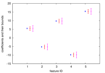
Let $\bm{e}_{j}\in\mathbb{R}^{d}$, $j\in[d]$, be a vector of all 0 except 1 in the $j^{\rm th}$ element. Then, by setting $\bm{\eta}:=\bm{e}_{j}$ in (5), we can compute a lower and an upper bounds of the new classifier’s coefficient $\beta^{*}_{{\rm new},j}=\bm{e}_{j}^{\top}\bm{\beta}^{*}_{\rm new},j\in[d]$ such that

$$L(\beta^{*}_{{\rm new},j})\leq\beta^{*}_{{\rm new},j}\leq U(\beta^{*}_{{\rm new},j}),~{}j\in[d].$$

Figure 1 illustrates such coefficient’s bounds for a simple toy dataset. Given a lower and an upper bounds of the coefficients, we can, in principle, obtain the bounds of any quantities depending on $\bm{\beta}^{*}_{\rm new}$. Bounding the largest possible change of the new classifier’s coefficients or a quantity depending on it would be beneficial for making decisions in practical tasks.

Figure 1: Examples of coefficient bounds $L(\beta^{*}_{{\rm new},j})$ and $U(\beta^{*}_{{\rm new},j})$, $j\in[5]$, for an artificial toy dataset with $n_{\rm old}=1000$ and $d=5$. The blue, red and pink error bars indicate the bounds when $n_{A}+n_{R}=1$ (0.1%), $5$ (0.5%), and $10$ (1%), respectively. The unknown true coefficients $\beta^{*}_{{\rm new},j}$, $j\in[5]$, are indicated by $\bm{\times}$.

2.3 Sensitivity of class labels

Next, let us consider sensitivity analysis of the new class label for a test instance $\bm{x}\in\mathbb{R}^{d}$, i.e., we would like to know

$$\hat{y}:={\text{sgn}}(f(\bm{x};\bm{\beta}^{*}_{\rm new}))={\text{sgn}}(\bm{x}^{\top}\bm{\beta}^{*}_{\rm new}).$$

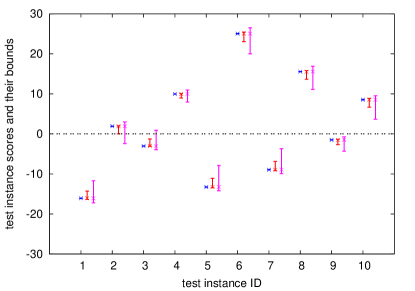
By setting $\bm{\eta}:=\bm{x}$ in (5), we can compute a lower and an upper bounds such that

$$L(\bm{x}^{\top}\bm{\beta}^{*}_{\text{new}})\leq\bm{x}^{\top}\bm{\beta}^{*}_{\text{new}}\leq U(\bm{x}^{\top}\bm{\beta}^{*}_{\text{new}}).$$ (6)

Here, it is interesting to note that, using the following simple facts:

$$L(\bm{x}^{\top}\bm{\beta}^{*}_{\text{new}})\geq 0~{}\Rightarrow~{}\hat{y}=+1,$$ (7a)

$$U(\bm{x}^{\top}\bm{\beta}^{*}_{\text{new}})<0~{}\Rightarrow~{}\hat{y}=-1,$$ (7b)

the class label $\hat{y}$ can be available without actually obtaining $\bm{\beta}^{*}_{\text{new}}$ if the bounds are sufficiently tight such that the signs of the lower and the upper bounds are same. If the number of updated instances $n_{A}+n_{R}$ is relatively smaller than the entire training set size $n_{\rm old}$ or $n_{\rm new}$, we expect that the two solutions $\bm{\beta}^{*}_{\rm old}$ and $\bm{\beta}^{*}_{\rm new}$ would not be so different. In such cases, as we demonstrate empirically in §5, the bounds in (6) are sufficiently tight in many cases. Figure 2 illustrates the tightness of the bounds in a toy dataset.

Figure 2: Examples of test instance score bounds $L(\bm{x}^{\top}\bm{\beta}^{*}_{{\rm new}})$ and $U(\bm{x}^{\top}\bm{\beta}^{*}_{{\rm new}})$ for 10 test instances in the same dataset as in Figure 1. The blue, red and pink error bars indicate the bounds when $n_{A}+n_{R}=1$ (0.1%), $5$ (0.5%), and $10$ (1%), respectively, and the unknown true scores $\bm{x}^{\top}\bm{\beta}^{*}_{\rm new}$ are indicated by $\bm{\times}$. Note that, except for the 2nd and the 3rd test instances with $n_{A}+n_{R}=10$ (pink), the signs of the lower and the upper bounds are same, meaning that the class labels of these test instances are immediately available without actually updating the classifier.

2.4 Leave-one-out cross-validation (LOOCV)

One of the traditional problem setups to which our proposed framework can be naturally applied is leave-one-out cross-validation (LOOCV). The LOOCV error is defined as

$$\text{LOOCV error}:=\frac{1}{n}\sum_{h\in[n]}I(y_{h}\neq\text{sgn}(\bm{x}^{\top}_{i}\bm{\beta}^{*}_{(-h)})),$$

where ${\rm sgn}(\cdot)$ is the sign, and $\bm{\beta}^{*}_{(-h)}$ is the optimal solution after leaving out the $h^{\rm th}$ instance, which is defined as

$$\bm{\beta}^{*}_{(-h)}:=\arg\min_{\bm{\beta}\in\mathbb{R}^{d}}~{}\frac{1}{n_{\rm old}-1}\sum_{i\in{\cal D}_{\rm old}\setminus\{h\}}\ell(y_{i},f(\bm{x}_{i},\bm{\beta}))+\frac{\lambda}{2}\|\bm{\beta}\|^{2}.$$

Here, our idea is to regard the solution obtained by the whole training set as $\bm{\beta}^{*}_{\text{old}}$, and $\bm{\beta}^{*}_{(-h)}$ as $\bm{\beta}^{*}_{\text{new}}$. By setting $\bm{\eta}:=y_{h}\bm{x}_{h}$ in (5), we can compute the bounds such that

$$L(y_{h}\bm{x}^{\top}_{h}\bm{\beta}^{*}_{(-h)})\leq y_{h}\bm{x}^{\top}_{h}\bm{\beta}^{*}_{(-h)}\leq U(y_{h}\bm{x}^{\top}_{h}\bm{\beta}^{*}_{(-h)}).$$ (8)

These bounds in (8) can be used to know whether the left out instance is correctly classified or not. If the lower bound is positive, the left-out instance will be correctly classified, while it will be mis-classified if the upper bound is negative.

Using (8), we can also obtain the bounds on the LOOCV error itself:

LOOCV error $$\geq\frac{1}{n}\sum_{h\in[n]}I\left(U(y_{h}\bm{x}^{\top}_{h}\bm{\beta}^{*}_{(-h)})<0\right),$$

LOOCV error $$\leq 1-\frac{1}{n}\sum_{h\in[n]}I\left(L(y_{h}\bm{x}^{\top}_{h}\bm{\beta}^{*}_{(-h)})>0\right),$$

where $I(\cdot)$ is the indicator function. In numerical experiments, we illustrate that this approach works quite well.

3 Quick sensitivity analysis

In this section we present our main results on our quick sensitivity analysis framework. The following theorem tells that we can compute a lower and an upper bounds of a general linear score $\bm{\eta}^{\top}\bm{\beta}^{*}_{\text{new}}$ by using the original solution $\bm{\beta}^{*}_{\text{old}}$.

Theorem 1.

Let

$$\bm{\Delta}s:=\frac{1}{n_{A}+n_{R}}\left(\sum_{i\in{\cal A}}\bm{\nabla}\ell_{i}(\bm{\beta}^{*}_{\text{old}})-\sum_{i\in{\cal R}}\bm{\nabla}\ell_{i}(\bm{\beta}^{*}_{\text{old}})\right).$$ (9)

Then, for an arbitrary vector $\bm{\eta}\in\mathbb{R}^{d}$, the linear score $\bm{\eta}^{\top}\bm{\beta}^{*}_{\text{new}}$ satisfies

$$\bm{\eta}^{\top}\bm{\beta}^{*}_{\text{new}}\geq L(\bm{\eta}^{\top}\bm{\beta}^{*}_{\text{new}})$$

$$~{}~{}~{}~{}~{}:=\frac{n_{\text{new}}+n_{\text{old}}}{2n_{\text{new}}}\bm{\eta}^{\top}\bm{\beta}^{*}_{\text{old}}-\lambda^{-1}\frac{n_{A}+n_{R}}{2n_{\text{new}}}\bm{\eta}^{\top}\bm{\Delta}s-\frac{1}{2}\|\bm{\eta}\|\left\|\frac{n_{A}-n_{R}}{n_{\text{new}}}\bm{\beta}^{*}_{\text{old}}+\lambda^{-1}\frac{n_{A}+n_{R}}{n_{\text{new}}}\bm{\Delta}s\right\|,$$ (10a)

$$\bm{\eta}^{\top}\bm{\beta}^{*}_{\text{new}}\leq U(\bm{\eta}^{\top}\bm{\beta}^{*}_{\text{new}})$$

$$~{}~{}~{}~{}~{}:=\frac{n_{\text{new}}+n_{\text{old}}}{2n_{\text{new}}}\bm{\eta}^{\top}\bm{\beta}^{*}_{\text{old}}-\lambda^{-1}\frac{n_{A}+n_{R}}{2n_{\text{new}}}\bm{\eta}^{\top}\bm{\Delta}s+\frac{1}{2}\|\bm{\eta}\|\left\|\frac{n_{A}-n_{R}}{n_{\text{new}}}\bm{\beta}^{*}_{\text{old}}+\lambda^{-1}\frac{n_{A}+n_{R}}{n_{\text{new}}}\bm{\Delta}s\right\|.$$ (10b)

The proof is presented in Appendix A.

An advantage of the bounds in (10) is that the computational complexity does not depend on the total number of instances, but only on the number of modified instances. It is easy to confirm that the main computational cost of these bounds is in the computation of $\bm{\Delta}s$ in (9), and its complexity is ${\cal O}((n_{A}+n_{R})d)$. The tightness of the bounds, i.e., the difference between the upper and the lower bounds is written as

$$U(\bm{\eta}^{\top}\bm{\beta}^{*}_{\text{new}})-L(\bm{\eta}^{\top}\bm{\beta}^{*}_{\text{new}})=\|\bm{\eta}\|\left\|\frac{n_{A}-n_{R}}{n_{\text{new}}}\bm{\beta}^{*}_{\text{old}}+\lambda^{-1}\frac{n_{A}+n_{R}}{n_{\text{new}}}\bm{\Delta}s\right\|.$$ (11)

In a typical sensitivity analysis where $n_{A}$ and $n_{R}$ are much smaller than $n_{\text{new}}$, the tightness in (11) would be small. Note also that the tightness depends inversely on the regularization parameter $\lambda$. If $\lambda$ is very small and close to zero, the bounds become very loose.

3.1 Sensitivity analysis of coefficients

As discussed in §2.2, by substituting $\bm{\eta}:=\bm{e}_{j}$, $j\in[d]$, into (10), we obtain a lower and an upper bounds of the $j^{\rm th}$ coefficient of the new classifier.

Corollary 2.

For $j\in[d]$, the $j^{\rm th}$ coefficient of the new classifier satisfies

$$\beta^{*}_{{\rm new},j}\geq L(\beta^{*}_{{\rm new},j})$$

$$~{}~{}~{}~{}~{}:=\frac{n_{\rm new}+n_{\rm old}}{2n_{\rm new}}\beta^{*}_{{\rm old},j}-\lambda^{-1}\frac{n_{A}+n_{R}}{2n_{\rm new}}\Delta s_{j}-\frac{1}{2}\Big{\|}\frac{n_{A}-n_{R}}{n_{\rm new}}\bm{\beta}^{*}_{{\rm old}}+\lambda^{-1}\frac{n_{A}+n_{R}}{n_{\rm new}}\bm{\Delta}s\Big{\|},$$ (12a)

$$\beta^{*}_{{\rm new},j}\leq U(\beta^{*}_{{\rm new},j})$$

$$~{}~{}~{}~{}~{}:=\frac{n_{\rm new}+n_{\rm old}}{2n_{\rm new}}\beta^{*}_{{\rm old},j}+\lambda^{-1}\frac{n_{A}+n_{R}}{2n_{\rm new}}\Delta s_{j}+\frac{1}{2}\Big{\|}\frac{n_{A}-n_{R}}{n_{\rm new}}\bm{\beta}^{*}_{{\rm old}}+\lambda^{-1}\frac{n_{A}+n_{R}}{n_{\rm new}}\bm{\Delta}s\Big{\|}.$$ (12b)

Note that the third term does not depend on $j\in[d]$, i.e., the tightness of the bounds in (12) is common for all the coefficients $\beta^{*}_{{\rm new},j}$, $j\in[d]$.

Given a lower and an upper bounds of the coefficients $\beta^{*}_{{\rm new},j}$, $j\in[d]$, we can obtain the bounds of any quantities depending on $\bm{\beta}^{*}_{\rm new}$. For example, it is straightforward to know how much the classifier’s coefficients can change by the incremental operation when the amount of the change is measured in terms of some norm of $\bm{\beta}^{*}_{\rm new}-\bm{\beta}^{*}_{\rm old}$.

Corollary 3.

For any $q>0$, let $\|\bm{z}\|_{q}$ be the $L_{q}$ norm of a vector $\bm{z}$. Then the difference between the old and the new classifier’s coefficients in $L_{q}$-norm is bounded from above as

$$\|\bm{\beta}^{*}_{\rm new}-\bm{\beta}^{*}_{\rm old}\|_{q}\leq\Bigl{(}\sum_{j\in[d]}\max\{\beta^{*}_{{\rm old},j}-L(\beta^{*}_{{\rm new},j}),U(\beta^{*}_{{\rm new},j})-\beta^{*}_{{\rm old},j}\}^{q}\Bigr{)}^{\frac{1}{q}}.$$ (13)

Some readers might note that a lower and an upper bounds of a general linear score $\bm{\eta}^{\top}\bm{\beta}^{*}_{\rm new}$ can be simply obtained by using the bounds of each coefficients $\beta^{*}_{{\rm new},j}$, $j\in[d]$. Such naive bounds are given as

$$\bm{\eta}^{\top}\bm{\beta}^{*}_{\rm new}\geq\tilde{L}(\bm{\eta}^{\top}\bm{\beta}^{*}_{\rm new}):=\sum_{j|\eta_{j}<0}\eta_{j}U(\beta^{*}_{{\rm new},j})+\sum_{j|\eta_{j}>0}\eta_{j}L(\beta^{*}_{{\rm new},j}),$$ (14a)

$$\bm{\eta}^{\top}\bm{\beta}^{*}_{\rm new}\leq\tilde{U}(\bm{\eta}^{\top}\bm{\beta}^{*}_{\rm new}):=\sum_{j|\eta_{j}<0}\eta_{j}L(\beta^{*}_{{\rm new},j})+\sum_{j|\eta_{j}>0}\eta_{j}U(\beta^{*}_{{\rm new},j}).$$ (14b)

The tightness of the bounds in (14) is written as

$$\tilde{U}(\bm{\eta}^{\top}\bm{\beta}^{*}_{\rm new})-\tilde{L}(\bm{\eta}^{\top}\bm{\beta}^{*}_{\rm new}):=\sum_{j\in[d]}|\eta_{j}|(U(\beta^{*}_{{\rm new},j})-L(\beta^{*}_{{\rm new},j})),$$

which is clearly much looser than (11). Thus, if the quantity of the interest is written in a linear score form $\bm{\eta}^{\top}\bm{\beta}^{*}_{\rm new}$, we should use the bounds in (10) rather than (14).

3.2 Sensitivity analysis of class labels

Next, we use Theorem 1 for sensitivity analysis of new class labels. As discussed in §2.3, for an input vector $\bm{x}\in\mathbb{R}^{d}$, we can obtain a lower and an upper bounds of a linear score $\bm{x}^{\top}\bm{\beta}^{*}_{\rm new}$ by setting $\bm{\eta}=\bm{x}$. From (7), we can know the new class label if the signs of the lower and the upper bounds are same.

Corollary 4.

Let $\bm{x}\in\mathbb{R}^{d}$ be an arbitrary $d$-dimensional input vector. Then, the classification result

$$\hat{y}:={\rm sgn}(f(\bm{x};\bm{\beta}^{*}_{\rm new}))={\rm sgn}(\bm{x}^{\top}\bm{\beta}^{*}_{\rm new})$$

satisfies

$$\hat{y}=\left\{\begin{array}[]{ll}+1&\text{if }L(\bm{x}^{\top}\bm{\beta}^{*}_{\rm new})>0,\\ -1&\text{if }U(\bm{x}^{\top}\bm{\beta}^{*}_{\rm new})<0,\\ \text{unknown}&\text{otherwise},\end{array}\right.$$

where

$$L(\bm{x}^{\top}\bm{\beta}^{*}_{\rm new}):=\frac{n_{\text{new}}+n_{\text{old}}}{2n_{\text{new}}}\bm{x}^{\top}\bm{\beta}^{*}_{\text{old}}-\lambda^{-1}\frac{n_{A}+n_{R}}{2n_{\text{new}}}\bm{x}^{\top}\bm{\Delta}s-\frac{1}{2}\|\bm{x}\|\left\|\frac{n_{A}-n_{R}}{n_{\text{new}}}\bm{\beta}^{*}_{\text{old}}+\lambda^{-1}\frac{n_{A}+n_{R}}{n_{\text{new}}}\bm{\Delta}s\right\|,$$

$$U(\bm{x}^{\top}\bm{\beta}^{*}_{\rm new}):=\frac{n_{\text{new}}+n_{\text{old}}}{2n_{\text{new}}}\bm{x}^{\top}\bm{\beta}^{*}_{\text{old}}-\lambda^{-1}\frac{n_{A}+n_{R}}{2n_{\text{new}}}\bm{x}^{\top}\bm{\Delta}s+\frac{1}{2}\|\bm{x}\|\left\|\frac{n_{A}-n_{R}}{n_{\text{new}}}\bm{\beta}^{*}_{\text{old}}+\lambda^{-1}\frac{n_{A}+n_{R}}{n_{\text{new}}}\bm{\Delta}s\right\|.$$

Corollary 4 is useful in transductive setups [19] where we are only interested in the class labels of the prespecified set of test inputs.

3.3 Quick leave-one-out cross-validation

In LOOCV, we repeat leaving out a single instance from the training set, and check whether it is correctly classified or not by the new classifier which is trained without the left-out instance. Thus, each step of LOOCV computation can be considered as an incremental operation with $n_{A}=0$ and $n_{R}=1$. Denoting the left-out instance as $(\bm{x}_{h},y_{h})$, $h\in[n_{\rm old}]$, the task is to inquire whether the left-out instance is correctly classified or not, which is known by checking the sign of $y_{h}f(\bm{x}_{h};\bm{\beta}^{*}_{\rm new})=y_{h}\bm{x}_{h}^{\top}\bm{\beta}^{*}_{\rm new}$.

Corollary 5.

Consider a single step of LOOCV computation where an instance $(\bm{x}_{h},y_{h}),h\in[n_{\rm old}]$, is left out. Then,

$$L(y_{h}f(\bm{x}_{h};\bm{\beta}^{*}_{\rm new}))>0~{}\Rightarrow~{}\text{$(\bm{x}_{h},y_{h})$ is correctly classified}$$

$$U(y_{h}f(\bm{x}_{h};\bm{\beta}^{*}_{\rm new}))<0~{}\Rightarrow~{}\text{$(\bm{x}_{h},y_{h})$ is mis-classified}$$

where

$$L(y_{h}f(\bm{x}_{h};\bm{\beta}^{*}_{\rm new}))$$

$$:=\frac{2n_{\rm old}-1}{2n_{\rm old}-2}y_{h}\bm{x}_{h}^{\top}\bm{\beta}^{*}_{\text{old}}+\frac{\lambda^{-1}}{2n_{\text{old}}-2}y_{h}\bm{x}_{h}^{\top}\bm{\nabla}\ell_{i}(\bm{\beta}^{*}_{\rm old})-\frac{1}{2}\|\bm{x}_{h}\|\left\|\frac{-1}{n_{\rm old}-1}\bm{\beta}^{*}_{\text{old}}+\frac{\lambda^{-1}}{n_{\rm old}-1}\bm{\nabla}\ell_{i}(\bm{\beta}^{*}_{\rm old})\right\|,$$ (15a)

$$U(y_{h}f(\bm{x}_{h};\bm{\beta}^{*}_{\rm new}))$$

$$:=\frac{2n_{\rm old}-1}{2n_{\rm old}-2}y_{h}\bm{x}_{h}^{\top}\bm{\beta}^{*}_{\text{old}}+\frac{\lambda^{-1}}{2n_{\text{old}}-2}y_{h}\bm{x}_{h}^{\top}\bm{\nabla}\ell_{i}(\bm{\beta}^{*}_{\rm old})+\frac{1}{2}\|\bm{x}_{h}\|\left\|\frac{-1}{n_{\rm old}-1}\bm{\beta}^{*}_{\text{old}}+\frac{\lambda^{-1}}{n_{\rm old}-1}\bm{\nabla}\ell_{i}(\bm{\beta}^{*}_{\rm old})\right\|.$$ (15b)

4 Tightening linear score bounds via a suboptimal solution

In the previous section we introduced a framework that can quickly compute a lower and an upper bounds of a linear score of the new classifier. Unfortunately, it is not always the case that these bounds are sufficiently tight for making a desired inference on the new classifier. For example, if the lower and the upper bounds of $\bm{x}^{\top}\bm{\beta}_{\rm new}^{*}$ do not have the same sign for a test input $\bm{x}$, we cannot tell which class it would be classified to. In this section we discuss how to deal with such a situation.

The simplest way to handle such a situation is just to use conventional incremental learning algorithms. If we completely solve the optimization problem (2) by an incremental learning algorithm, we can obtain $\bm{\beta}_{\rm new}^{*}$ itself. However, if our goal is only to make a particular inference about the new classifier, we do not have to solve the optimization problem (2) completely until convergence. In this section we propose a similar framework for computing a lower and an upper bounds of a linear score by using a suboptimal solution before convergence which would be obtained during the optimization of problem (2).

We denote such a suboptimal solution as $\hat{\bm{\beta}}_{\rm new}$. In order to compute the bounds, we use the gradient information of the problem (2), which we denote

$$\bm{g}(\hat{\bm{\beta}}_{\rm new}):=\frac{1}{n_{\rm new}}\sum_{i\in{\cal D}_{\rm new}}\bm{\nabla}\ell_{i}(\hat{\bm{\beta}}_{\rm new})+\lambda\hat{\bm{\beta}}_{\rm new}.$$ (16)

The complexity of computing the gradient vector from scratch is ${\cal O}(n_{\rm new}d)$. However, if we are using a gradient-based optimization algorithm such as conjugate gradient or quasi-Newton methods, we should have already computed the gradient vector in each iteration of the optimization algorithm. The following theorem provides a lower and an upper bound of a linear score by using the current gradient information. If we already have computed $\bm{g}(\hat{\bm{\beta}}_{\rm new})$, these bounds can be obtained very cheaply.

Theorem 6.

For an arbitrary vector $\bm{\eta}\in\mathbb{R}^{d}$, the linear score $\bm{\eta}^{\top}\bm{\beta}^{*}_{\text{new}}$ satisfies

$$\bm{\eta}^{\top}\bm{\beta}^{*}_{\text{new}}\geq\hat{L}(\bm{\eta}^{\top}\bm{\beta}^{*}_{\text{new}}):=\bm{\eta}^{\top}\hat{\bm{\beta}}_{\rm new}-\frac{\lambda^{-1}}{2}\bm{\eta}^{\top}\bm{g}(\hat{\bm{\beta}}_{\rm new})-\frac{\lambda^{-1}}{2}\|\bm{\eta}\|\|\bm{g}(\hat{\bm{\beta}}_{\rm new})\|,$$ (17a)

$$\bm{\eta}^{\top}\bm{\beta}^{*}_{\text{new}}\leq\hat{U}(\bm{\eta}^{\top}\bm{\beta}^{*}_{\text{new}}):=\bm{\eta}^{\top}\hat{\bm{\beta}}_{\rm new}-\frac{\lambda^{-1}}{2}\bm{\eta}^{\top}\bm{g}(\hat{\bm{\beta}}_{\rm new})+\frac{\lambda^{-1}}{2}\|\bm{\eta}\|\|\bm{g}(\hat{\bm{\beta}}_{\rm new})\|.$$ (17b)

The proof is presented in Appendix A.

A nice property of the bounds in (17) is that the tightness

$$\hat{U}(\bm{\eta}^{\top}\bm{\beta}^{*}_{\text{new}})-\hat{L}(\bm{\eta}^{\top}\bm{\beta}^{*}_{\text{new}})=\lambda^{-1}\|\bm{\eta}\|\|\bm{g}(\hat{\bm{\beta}}_{\rm new})\|$$

is linear in the norm of the gradient $\|\bm{g}(\hat{\bm{\beta}}_{\rm new})\|$. It means that, as the optimization algorithm for (2) proceeds, the gap between the lower and the upper bounds in (17) decreases, and it converges to zero as the solution converges to the optimal one. Theorem 6 can be used as a stopping criterion for incremental learning optimization problem (2). For example, in a sensitivity analysis of class labels, one can proceed the optimization process until the signs of the lower and the upper bounds in (17) become same.

5 Numerical experiments

In this section we describe numerical experiments. In §5.1 we illustrate the tightness and the computational efficiency of our bounds in two sensitivity analysis tasks described in §2.2 and §2.3. In §5.2 we apply our framework to LOOCV computation as described in §2.4 and compare its performance with conventional LOOCV computation methods.

Table 1 summarizes the datasets used in the experiments. They are all taken from libsvm dataset repository [4]. For the experiments in §5.1, we used larger datasets D5-D8. For LOOCV experiments in §5.2, we used smaller datasets D1-D4. As examples of the loss function $\ell$, we used LR loss (3) and SVM loss (4). In §5.1 we only show the results on logistic regression. In §5.2 we compare our results on SVMs with conventional LOOCV methods particularly designed for SVMs. For logistic regression, we only compare our framework with conventional incremental learning algorithm because there is no particular LOOCV computation method for logistic regression. As an incremental learning algorithm, which is used as competitor and as a part of our algorithm for LOOCV computation, we used the approach in [18]. All the computations were conducted by using a single core of an HP workstation Z820 (Xeon(R) CPU E5-2693 (3.50GHz), 64GB MEM).

Table 1: Benchmark datasets used in the experiments.

	dataset name	$n_{\rm train}$	$d$	$n_{\rm test}$
D1	sonar	208	60	not used
D2	splice	1000	60	not used
D3	w5a	9888	300	not used
D4	a7a	16100	123	not used
D5	a9a	32561	123	16281
D6	ijcnn	49990	22	91701
D7	cod-rna	59535	8	271617
D8	kdd2010	$>$ 8 million	$>$20 million	$>$ 0.5 million

5.1 Results on two sensitivity analysis tasks

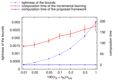
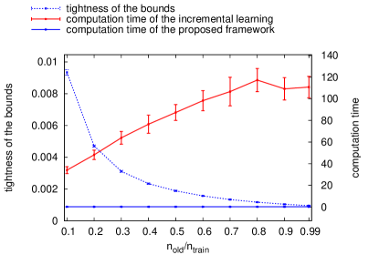
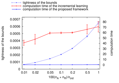
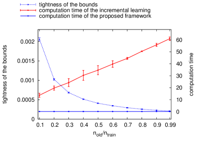
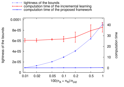
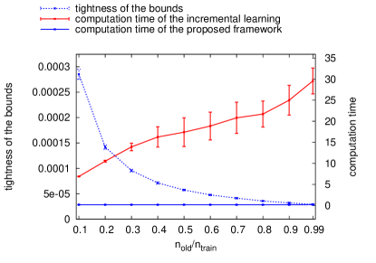
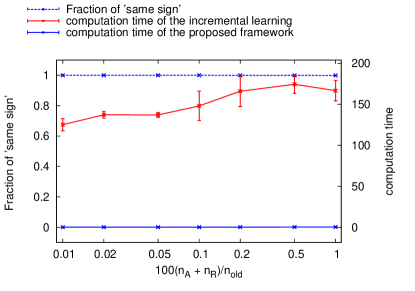
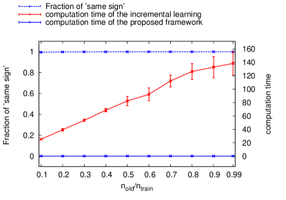
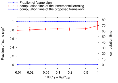
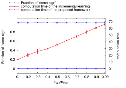
Here we show the results on two sensitivity analysis tasks described in §2.2 and §2.3. We empirically evaluate the tightness of the bounds and the computational costs for larger datasets D5-D8. First, we see how the results change as the number of added and/or removed instances changes among $n_{A}+n_{R}\in\{0.01\%$, $0.02\%$, $0.05\%$, $0.1\%$, $0.2\%$, $0.5\%$, $1\%\}$ of the entire training set size $n_{\rm old}$. Next, we see the results when the number of the entire training set size changes among $n_{\rm old}\in\{10\%$, $20\%$, $\ldots$, $90\%$, $99\%\}$ of $n_{\rm train}$, while the number of added and/or removed instances is fixed to $n_{A}+n_{R}=0.001n_{\rm train}$.

In the first sensitivity analysis task about coefficients (see §2.2 and §3.1), we simply computed the difference between the upper and the lower bounds $U(\beta_{{\rm new},j}^{*})-L(\beta_{{\rm new},j}^{*})$ for evaluating the tightness of the bounds. For the second sensitivity analysis task about class labels (see §2.3 and §3.2), we examined the percentage of the test instances for which the signs of the lower and the upper bounds are same. Remember that the class label can be immediately available when the lower and the upper bounds have same sign.

Tables 2 - 7 show the results for the former task. (Figure 3 depicts the results on D8 as an example). These results indicate that the bounds are fairly tight if the $n_{A}+n_{R}$ is relatively smaller than $n_{\rm old}$. The computational costs of our proposed framework (blue thick curves) are negligible compared with the costs of actual incremental learning (red thick curves).

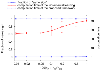
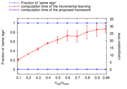
Tables 8 - 13 show the results for the latter task (Figure 4 depicts the results on D8 as an example). The results here indicate that, in most cases, the bounds are sufficiently tight for making the signs of the lower and the upper bounds same. It means that, in most cases, the new class labels after incremental operation are available without actually updating the classifier itself.

The results presented here were obtained with the regularization parameter $\lambda=0.01,0.1,1$. We observed that, for larger $\lambda$, the bounds became tighter. These all experiment results are mean and variance of performing 30 times.

Algorithm 1 Proposed LOOCV method (op1)

0:  $\{(\bm{x}_{i},y_{i})\}_{i\in[n_{\rm old}]}$

1:  $\bm{\beta}_{\rm all}^{*}\leftarrow$solve (1), $h\leftarrow 1$, $err\leftarrow 0$

2:  while $h\leq n_{\rm old}$ do

3:     if $U(y_{h}f(\bm{x}_{h};\bm{\beta}^{*}_{(-h)})<0$ then

4:        $err\leftarrow err+1$

5:     else if $L(y_{h}f(\bm{x}_{h};\bm{\beta}^{*}_{(-h)})<0$ then

6:        $\bm{\beta}_{(-h)}^{*}\leftarrow$solve (2) by incremental learning algorithm

7:        if $y_{h}\bm{x}_{h}^{\top}\bm{\beta}^{*}_{(-h)}<0$ then

8:           $err\leftarrow err+1$

9:        end if

10:     end if

11:     $h\leftarrow h+1$

12:  end while

12:  LOOCV error: $err/n_{\rm old}$

5.2 Leave-one-out cross-validation

We applied the proposed framework to LOOCV task, and compare its computational efficiency with existing approaches. We consider two options. In the first option (op1), we only used the method described in §3.3. In the second option (op2), we also used the method described in §4. Algorithm 1 is the pseudo-code for computing LOOCV errors by using the proposed framework with op1. Briefly speaking, for each of the left-out instance $(\bm{x}_{h},y_{h})$, we first compute the lower and the upper bounds of $y_{h}f(\bm{x}_{h};\bm{\beta}^{*}_{(-h)})$. Then, if the lower/upper bound is greater/smaller than zero, we confirm that the instance is correctly/incorrectly classified. When the signs of the two bounds are different, the class label is unknown. In such a case, we use conventional incremental learning algorithm in [18]. In op1, we ran the incremental learning algorithm until its convergence and obtain $\bm{\beta}^{*}_{(-h)}$ itself. In op2, we stopped the optimization process at which the signs of the bounds in (17) became same.

For SVMs, several LOOCV methods have been studied in the literature [19, 10]. For the experiments with SVM loss, we thus compare our approach with the methods in [19] and [10]. The former approach merely exploits the fact that adding and/or removing non-support vectors does not change the classifier. The method called $\xi\text{-}\alpha$ estimator [10] also provides a lower bound of $y_{h}f(\bm{x}_{h};\bm{\beta}^{*}_{\rm new})$ without actually obtaining $\bm{\beta}^{*}_{\rm new}$. For the experiments with logistic regression loss, we compare our approaches only with incremental learning approach [18] because there are no other competing methods.

We used the above LOOCV computation methods in model selection tasks for linear and nonlinear classification problems. In linear case, the task is to find the regularization parameter $\lambda\in\{2^{-20},2^{-19},\ldots,2^{0}\}$ that minimizes the LOOCV error. In nonlinear case, we used Gaussian RBF in the form of $\phi_{k}(\bm{x})=\exp(-\gamma\|\bm{x}-\bm{x}_{k}\|^{2})$, where $k\in[100]$ were randomly selected from $[n_{\rm old}]$. Here, the task is to select the optimal combination of $(\lambda,\gamma)\in\{2^{-15},2^{-14},\ldots,2^{-5}\}\times\{2^{-5},2^{-4},\ldots,2^{5}\}$ that minimizes the LOOCV error.

For further speed-up, we also conducted experiments with two simple tricks. In the first trick we used the lower and the upper bounds of the LOOCV error itself. If the lower bound of one model is greater than the upper bound of another model, the former model would never be selected as the best model, meaning that the LOOCV error computation process can be stopped. The second simple trick is to conduct incremental learning operations in the increasing order of $y_{h}f(\bm{x}_{h};\bm{\beta}^{*}_{\rm old})$. It is based on a simple observation that the class label of an instance whose $y_{h}f(\bm{x}_{h};\bm{\beta}^{*}_{\rm old})$ value is small tends to be mis-classified. Note that these two tricks can be used not only for our proposed framework, but also for other competing approaches.

Tables 14 and 15 show the results without and with the tricks, respectively. We see that the computational cost of our proposed framework (especially op2) are much smaller than competing methods. It indicates that our bounds in (15) is tighter in many cases than the existing bounds for LOOCV error computation.

6 Conclusions and future works

In this paper we introduced a novel framework for sensitivity analysis of large scale classification problems. The proposed framework provides a lower and an upper bounds of a general linear score on the updated classifier without actually re-optimized it. The advantage of the proposed framework is that the computational cost only depends on the sizes of the modified instances, which is particularly advantageous in typical sensitivity analysis task where only relatively small number of instances are updated. We discussed three tasks to which the proposed framework can be applied. As a future work, we plan to apply the proposed framework to stream learning.

7 Acknowledgement

For this work, IT was partially supported by JST CREST, MEXT Kakenhi 26106513, and MEXT Kakenhi 26106513.

Appendix A Proofs

In this section we prove Theorems 1 and 6. First we present the following proposition.

Proposition 7.

Consider the following general problem:

$$\min_{z}~{}\phi(z)~{}~{}~{}{\rm s.t.}~{}z\in{\cal Z},$$ (18)

where $\phi:{\cal Z}\to\mathbb{R}$ is a differentiable convex function and ${\cal Z}$ is a convex set. Then a solution $z^{*}$ is the optimal solution of (18) if and only if

$$\nabla\phi(z^{*})^{\top}(z^{*}-z)\leq 0~{}~{}~{}\forall~{}z\in{\cal Z},$$

where $\nabla\phi(z^{*})$ is the gradient vector of $\phi$ at $z=z^{*}$.

See, for example, Proposition 2.1.2 in [1] or Section 4.2.3 in [2] for the proof of Proposition 7.

Proof of Theorem 1.

From Proposition 7 and the optimality of $\bm{\beta}^{*}_{\rm new}$ for the problem (2)

$$\!\!\!\!\!\!\!\!\bigg{(}\frac{1}{n_{\rm new}}\sum_{i\in{\cal D}_{\rm new}}\bm{\nabla}\ell_{i}(\bm{\beta}^{*}_{\rm new})+\lambda\bm{\beta}^{*}_{\rm new}\bigg{)}^{\top}(\bm{\beta}^{*}_{\rm new}-\bm{\beta}^{*}_{\rm old})\leq 0.$$ (19)

From the convexity of $\ell_{i}$,

$$\ell_{i}(\bm{\beta}^{*}_{\rm old})\>\geq\ell_{i}(\bm{\beta}^{*}_{\rm new})+\bm{\nabla}\ell_{i}(\bm{\beta}^{*}_{\rm new})^{\top}(\bm{\beta}^{*}_{\rm old}-\bm{\beta}^{*}_{\rm new}),$$ (20)

$$\ell_{i}(\bm{\beta}^{*}_{\rm new})\geq\ell_{i}(\bm{\beta}^{*}_{\rm old\>})+\bm{\nabla}\ell_{i}(\bm{\beta}^{*}_{\rm old\>})^{\top}(\bm{\beta}^{*}_{\rm new}-\bm{\beta}^{*}_{\rm old}).$$ (21)

Using (20) and (21),

$$\bm{\nabla}\ell_{i}(\bm{\beta}^{*}_{\rm new})^{\top}(\bm{\beta}^{*}_{\rm new}-\bm{\beta}^{*}_{\rm old})\geq\bm{\nabla}\ell_{i}(\bm{\beta}^{*}_{\rm old\>})^{\top}(\bm{\beta}^{*}_{\rm new}-\bm{\beta}^{*}_{\rm old}).$$ (22)

By summing up (22) for all $i\in{\cal D}_{\rm new}$,

$$\sum_{i\in{\cal D}_{\rm new}}\bm{\nabla}\ell_{i}(\bm{\beta}^{*}_{\rm new})^{\top}(\bm{\beta}^{*}_{\rm new}-\bm{\beta}^{*}_{\rm old})\geq\sum_{i\in{\cal D}_{\rm new}}\bm{\nabla}\ell_{i}(\bm{\beta}^{*}_{\rm old\>})^{\top}(\bm{\beta}^{*}_{\rm new}-\bm{\beta}^{*}_{\rm old}).$$ (23)

Substituting (23) into (19),

$$\!\!\!\!\!\!\!\!\frac{1}{n_{\rm new}}\sum_{i\in{\cal D}_{\rm new}}\bm{\nabla}\ell_{i}(\bm{\beta}^{*}_{\rm old})^{\top}(\bm{\beta}^{*}_{\rm new}-\bm{\beta}^{*}_{\rm old})+\lambda\bm{\beta}^{*\top}_{\rm new}(\bm{\beta}^{*}_{\rm new}-\bm{\beta}^{*}_{\rm old})\leq 0.$$ (24)

By completing the square of (24), we have

$$\Bigg{\|}\bm{\beta}^{*}_{\rm new}-\frac{1}{2}\Bigg{(}\bm{\beta}^{*}_{\rm old}-\frac{\lambda^{-1}}{n_{\rm new}}\sum_{i\in{\cal D}_{\rm new}}\bm{\nabla}\ell_{i}(\bm{\beta}^{*}_{\rm old})\Bigg{)}\Bigg{\|}^{2}\leq\Bigg{(}\frac{1}{2}\Bigg{\|}\bm{\beta}^{*}_{\rm old}+\frac{\lambda^{-1}}{n_{\rm new}}\sum_{i\in{\cal D}_{\rm new}}\bm{\nabla}\ell_{i}(\bm{\beta}^{*}_{\rm old})\Bigg{\|}\Bigg{)}^{2}.$$ (25)

Furthermore, noting that $\bm{\beta}^{*}_{\rm old}$ is the optimal solution of (1),

$$\bm{\beta}^{*}_{\rm old}+\frac{\lambda^{-1}}{n_{\rm old}}\sum_{i\in{\cal D}_{\rm old}}\nabla\ell_{i}(\bm{\beta}^{*}_{\rm old})=0.$$ (26)

Using (26) and (9),

$$\frac{\lambda^{-1}}{n_{\rm new}}\sum_{i\in{\cal D}_{\rm new}}\bm{\nabla}\ell_{i}(\bm{\beta}^{*}_{\rm old}) =\frac{\lambda^{-1}}{n_{\rm new}}\Bigg{(}\sum_{i\in{\cal D}_{\rm old}}\bm{\nabla}\ell_{i}(\bm{\beta}^{*}_{\rm old})+\sum_{i\in{\cal A}}\bm{\nabla}\ell_{i}(\bm{\beta}^{*}_{\rm old})-\sum_{i\in{\cal R}}\bm{\nabla}\ell_{i}(\bm{\beta}^{*}_{\rm old})\Bigg{)}$$

$$=\frac{\lambda^{-1}}{n_{\rm new}}\Bigg{(}-\lambda n_{\rm old}\bm{\beta}^{*}_{\rm old}+(n_{A}+n_{R})\bm{\Delta}s\Bigg{)}$$

$$=-\frac{n_{\rm old}}{n_{\rm new}}\bm{\beta}^{*}_{\rm old}+\frac{(n_{A}+n_{R})\lambda^{-1}}{n_{\rm new}}\bm{\Delta}s$$ (27)

Substituting (27) into (25),

$$\Bigg{\|}\bm{\beta}^{*}_{\rm new}-\Bigg{(}\frac{n_{\rm old}+n_{\rm new}}{2n_{\rm new}}\bm{\beta}^{*}_{\rm old}-\frac{(n_{A}+n_{R})\lambda^{-1}}{2n_{\rm new}}\bm{\Delta}s\Bigg{)}\Bigg{\|}^{2}\leq\Bigg{(}\frac{1}{2}\Bigg{\|}\frac{n_{A}-n_{R}}{n_{\rm new}}\bm{\beta}^{*}_{\rm old}+\frac{(n_{A}+n_{R})\lambda^{-1}}{n_{\rm new}}\bm{\Delta}s\Bigg{\|}\Bigg{)}^{2}$$ (28)

Let

$$\bm{m}=\frac{n_{\rm old}+n_{\rm new}}{2n_{\rm new}}\bm{\beta}^{*}_{\rm old}-\frac{(n_{A}+n_{R})\lambda^{-1}}{2n_{\rm new}}\bm{\Delta}s~{},~{}r=\frac{1}{2}\Bigg{\|}\frac{n_{A}-n_{R}}{n_{\rm new}}\bm{\beta}^{*}_{\rm old}+\frac{(n_{A}+n_{R})\lambda^{-1}}{n_{\rm new}}\bm{\Delta}s\Bigg{\|}.$$ (29)

Then, (29) is compactly written as

$$\bm{\beta}^{*}_{\rm new}\in\Omega,\text{ where }\Omega:=\{\bm{\beta}~{}|~{}\|\bm{\beta}-\bm{m}\|^{2}\leq r^{2}\}.$$ (30)

Eq. (30) indicates that the new optimal solution $\bm{\beta}^{*}_{\rm new}$ is within a ball with center $\bm{m}$ and radius $r$. Thus, we have a lower and an upper bounds of a linear score $\bm{\eta}^{\top}\bm{\beta}^{*}_{\rm new}$ as follows:

$$L(\bm{\eta}^{\top}\bm{\beta}^{*}_{\rm new}) :=\min_{\bm{\beta}\in\Omega}~{}\bm{\eta}^{\top}\bm{\beta},$$ (31)

$$U(\bm{\eta}^{\top}\bm{\beta}^{*}_{\rm new}) :=\max_{\bm{\beta}\in\Omega}~{}\bm{\eta}^{\top}\bm{\beta}.$$ (32)

In fact, the solutions of (31) and (32) can be analytically obtained, and thus the lower bound $L(\bm{\eta}^{\top}\bm{\beta}^{*}_{\rm new})$ and the upper bound $U(\bm{\eta}^{\top}\bm{\beta}^{*}_{\rm new})$ can be explicitly obtained by using Lagrange multiplier method. Using a Lagrange multiplier $\alpha>0$, the problem (31) is rewritten as

$$\min_{\bm{\beta}}~{}\bm{\eta}^{\top}\bm{\beta}~{}~{}~{}{\rm s.t.}~{}\|\bm{\beta}-\bm{m}\|^{2}\leq r^{2}$$

$$= \min_{\bm{\beta}}\max_{\alpha>0}\big{(}\bm{\eta}^{\top}\bm{\beta}+\alpha(\|\bm{\beta}-\bm{m}\|^{2}-r^{2})\big{)}$$

$$= \max_{\alpha>0}\big{(}-\alpha r^{2}+\min_{\bm{\beta}}\big{(}\alpha\|\bm{\beta}-\bm{m}\|^{2}+\bm{\eta}^{\top}\bm{\beta}\big{)}\big{)}$$

$$= \max_{\alpha>0}~{}H(\alpha):=\big{(}-\alpha r^{2}-\frac{\|\bm{\eta}\|^{2}}{4\alpha}+\bm{\eta}^{\top}\bm{m}\big{)},$$

where $\alpha$ is strictly positive because the constraint $\|\bm{\beta}-\bm{m}\|^{2}\leq r^{2}$ is strictly active at the optimal solution. By letting $\partial H(\alpha)/\partial\alpha=0$, the optimal $\alpha$ is written as

$$\alpha^{*}:=\frac{\|\bm{\eta}\|}{2r}=\arg\max_{\alpha>0}~{}H(\alpha).$$

Substituting $\alpha^{*}$ into $H(\alpha)$,

$$\bm{\eta}^{\top}\bm{m}-\|\bm{\eta}\|r=\max_{\alpha>0}~{}H(\alpha).$$

Therefore,

$$L(\bm{\eta}^{\top}\bm{\beta}^{*}_{\rm new}) =\min_{\bm{\beta}\in\Omega}~{}\bm{\eta}^{\top}\bm{\beta}=\bm{\eta}^{\top}\bm{m}-\|\bm{\eta}\|r$$ (33)

The upper bound of $\bm{\eta}^{\top}\bm{\beta}$ in (32) can be similarly obtained as

$$U(\bm{\eta}^{\top}\bm{\beta}^{*}_{\rm new}) =\max_{\bm{\beta}\in\Omega}~{}\bm{\eta}^{\top}\bm{\beta}=\bm{\eta}^{\top}\bm{m}+\|\bm{\eta}\|r.$$ (34)

By substituting $\bm{m}$ and $r$ in (29) into (33) and (34), we have (10a) and (10b). ∎

Theorem 6 can be shown in a similar way as above.

Proof of Theorem 6.

From Proposition 7 and the optimality of $\bm{\beta}^{*}_{\rm new}$,

$$\!\!\!\!\!\!\!\!\bigg{(}\frac{1}{n_{\rm new}}\sum_{i\in{\cal D}_{\rm new}}\bm{\nabla}\ell_{i}(\bm{\beta}^{*}_{\rm new})+\lambda\bm{\beta}^{*}_{\rm new}\bigg{)}^{\top}(\bm{\beta}^{*}_{\rm new}-\hat{\bm{\beta}}_{\rm new})\leq 0.$$ (35)

From the convexity of $\ell_{i}$,

$$\ell_{i}(\bm{\beta}^{*}_{\rm new})\geq\ell_{i}(\hat{\bm{\beta}}_{\rm new})+\bm{\nabla}\ell_{i}(\hat{\bm{\beta}}_{\rm new})^{\top}(\bm{\beta}^{*}_{\rm new}-\hat{\bm{\beta}}_{\rm new}).$$ (36)

$$\ell_{i}(\hat{\bm{\beta}}_{\rm new})\geq\ell_{i}(\bm{\beta}^{*}_{\rm new})+\bm{\nabla}\ell_{i}(\bm{\beta}^{*}_{\rm new})^{\top}(\hat{\bm{\beta}}_{\rm new}-\bm{\beta}^{*}_{\rm new}).$$ (37)

Using (36) and (37) and the definition of $\bm{g}(\hat{\bm{\beta}}_{\rm new})$, the inequality (35) can be rewritten as the following condition on the new optimal solution $\bm{\beta}^{*}_{\rm new}$:

$$\bm{\beta}^{*}_{\rm new}\in\hat{\Omega},$$ (38)

where

$$\hat{\Omega}:=\Bigg{\{}\bm{\beta}\Bigg{|}~{}\Bigg{\|}\bm{\beta}-\Bigg{(}\hat{\bm{\beta}}_{\rm new}-\frac{\lambda^{-1}}{2}\bm{g}(\hat{\bm{\beta}}_{\rm new})\Bigg{)}\Bigg{\|}^{2}\leq\Bigg{(}\frac{\lambda^{-1}}{2}\|\bm{g}(\hat{\bm{\beta}}_{\rm new})\|\Bigg{)}^{2}\Bigg{\}}.$$

Then, the lower and the upper bounds in (17) are obtained by solving the following minimization and maximization problems

$$L(\bm{\eta}^{\top}\bm{\beta}^{*}_{\rm new}) :=\min_{\bm{\beta}\in\hat{\Omega}}~{}\bm{\eta}^{\top}\bm{\beta},$$ (39)

$$U(\bm{\eta}^{\top}\bm{\beta}^{*}_{\rm new}) :=\max_{\bm{\beta}\in\hat{\Omega}}~{}\bm{\eta}^{\top}\bm{\beta}.$$ (40)

Using the standard Lagrange multiplier method, the solutions of (39) and (40) are analytically obtained as (17a) and (17b), respectively. ∎

Figure 3: Results on sensitivity analysis of coefficients for D8. The tightness of the bounds and the computation time in seconds are plotted for $\lambda=0.01$ (top), $0.1$ (middle), and $1$ (bottom).

Figure 4: Results on sensitivity analysis of class labels for D8. The fraction of the test instances whose lower and upper bounds of the decision score have same signs, and the computation time in seconds are plotted for $\lambda=0.01$ (top), $0.1$ (middle), and $1$ (bottom).

		$(n_{\rm A}+n_{\rm R})/n_{\rm old}$
		$0.01\%$		$0.1\%$		$1\%$
		Incremental	proposed	Incremental	proposed	Incremental	proposed
D5	tightness	N.A.	5.68e-03	N.A.	1.94e-02	N.A.	6.63e-02
			($\pm$3.29e-03)		($\pm$5.69e-03)		($\pm$1.72e-02)
	time [sec]	4.57e-02	4.47e-06	5.41e-02	2.26e-05	6.16e-02	1.95e-04
		($\pm$6.38e-03)	($\pm$4.99e-07)	($\pm$2.37e-03)	($\pm$4.96e-07)	($\pm$5.32e-03)	($\pm$7.45e-07)
D6	tightness	N.A.	1.31e-03	N.A.	5.08e-03	N.A.	1.56e-02
			($\pm$8.35e-04)		($\pm$9.33e-04)		($\pm$2.92e-03)
	time [sec]	8.42e-02	6.37e-06	8.58e-02	3.21e-05	9.97e-02	2.84e-04
		($\pm$1.87e-02)	($\pm$2.50e-06)	($\pm$8.23e-03)	($\pm$1.38e-06)	($\pm$1.73e-02)	($\pm$7.55e-06)
D7	tightness	N.A.	2.00e-03	N.A.	6.83e-03	N.A.	2.27e-02
			($\pm$7.78e-04)		($\pm$2.33e-03)		($\pm$9.20e-03)
	time [sec]	1.30e-01	6.47e-06	1.65e-01	3.03e-05	1.90e-01	2.38e-04
		($\pm$2.88e-02)	($\pm$1.18e-06)	($\pm$2.13e-02)	($\pm$3.34e-06)	($\pm$2.36e-02)	($\pm$2.31e-05)
D8	tightness	N.A.	2.98e-04	N.A.	9.45e-04	N.A.	2.98e-03
			($\pm$8.96e-06)		($\pm$2.11e-05)		($\pm$3.89e-05)
	time [sec]	8.51e+01	1.53e-01	1.32e+02	1.82e-01	1.78e+02	3.59e-01
		($\pm$3.00e+00)	($\pm$8.24e-03)	($\pm$1.13e+01)	($\pm$1.17e-02)	($\pm$2.13e+01)	($\pm$1.63e-02)

Table 2: Results on sensitivity analysis of coefficients for various values of $(n_{\rm A}+n_{\rm R})/n_{\rm old}$. The tightness of the bounds and the computation time in seconds are listed ($\lambda=0.01$).

		$(n_{\rm A}+n_{\rm R})/n_{\rm old}$
		$0.01\%$		$0.1\%$		$1\%$
		Incremental	proposed	Incremental	proposed	Incremental	proposed
D5	tightness	N.A.	7.55e-04	N.A.	2.27e-03	N.A.	6.49e-03
			($\pm$3.74e-04)		($\pm$1.26e-03)		($\pm$1.83e-03)
	time [sec]	3.03e-02	4.13e-06	4.29e-02	2.21e-05	4.45e-02	1.94e-04
		($\pm$3.24e-03)	($\pm$4.27e-07)	($\pm$4.89e-03)	($\pm$6.29e-07)	($\pm$1.85e-03)	($\pm$8.23e-07)
D6	tightness	N.A.	1.86e-04	N.A.	6.54e-04	N.A.	2.09e-03
			($\pm$3.86e-05)		($\pm$1.10e-04)		($\pm$3.62e-04)
	time [sec]	3.17e-02	4.63e-06	6.49e-02	3.09e-05	6.60e-02	2.80e-04
		($\pm$7.71e-03)	($\pm$8.36e-07)	($\pm$6.65e-03)	($\pm$1.45e-06)	($\pm$7.14e-03)	($\pm$6.50e-06)
D7	tightness	N.A.	2.14e-04	N.A.	6.60e-04	N.A.	2.34e-03
			($\pm$7.57e-05)		($\pm$2.80e-04)		($\pm$9.89e-04)
	time [sec]	8.41e-02	6.30e-06	1.02e-01	3.08e-05	1.13e-01	2.31e-04
		($\pm$1.47e-02)	($\pm$9.36e-07)	($\pm$1.45e-02)	($\pm$4.94e-06)	($\pm$1.42e-02)	($\pm$1.43e-05)
D8	tightness	N.A.	6.56e-05	N.A.	2.07e-04	N.A.	6.50e-04
			($\pm$1.65e-06)		($\pm$3.94e-06)		($\pm$1.57e-05)
	time [sec]	4.11e+01	1.61e-01	5.96e+01	1.72e-01	7.11e+01	3.53e-01
		($\pm$4.95e+00)	($\pm$1.03e-02)	($\pm$1.50e+00)	($\pm$8.33e-03)	($\pm$9.80e+00)	($\pm$1.15e-02)

Table 3: Results on sensitivity analysis of coefficients for various values of $(n_{\rm A}+n_{\rm R})/n_{\rm old}$. The tightness of the bounds and the computation time in seconds are listed ($\lambda=0.1$).

		$(n_{\rm A}+n_{\rm R})/n_{\rm old}$
		$0.01\%$		$0.1\%$		$1\%$
		Incremental	proposed	Incremental	proposed	Incremental	proposed
D5	tightness	N.A.	7.49e-05	N.A.	2.56e-04	N.A.	7.47e-04
			($\pm$1.61e-05)		($\pm$6.87e-05)		($\pm$1.85e-04)
	time [sec]	1.45e-02	4.10e-06	1.89e-02	2.08e-05	2.26e-02	1.88e-04
		($\pm$1.55e-03)	($\pm$9.07e-07)	($\pm$3.25e-03)	($\pm$2.32e-06)	($\pm$8.96e-04)	($\pm$3.75e-06)
D6	tightness	N.A.	2.09e-05	N.A.	8.19e-05	N.A.	2.50e-04
			($\pm$3.84e-06)		($\pm$1.53e-05)		($\pm$4.33e-05)
	time [sec]	2.12e-02	4.83e-06	2.23e-02	3.02e-05	2.10e-02	2.70e-04
		($\pm$1.49e-03)	($\pm$1.29e-06)	($\pm$8.73e-04)	($\pm$9.45e-07)	($\pm$3.08e-03)	($\pm$5.53e-06)
D7	tightness	N.A.	1.93e-05	N.A.	8.59e-05	N.A.	2.21e-04
			($\pm$7.66e-06)		($\pm$3.95e-05)		($\pm$7.66e-05)
	time [sec]	1.95e-02	4.03e-06	2.50e-02	2.39e-05	2.86e-02	2.11e-04
		($\pm$7.41e-04)	($\pm$4.82e-07)	($\pm$5.21e-03)	($\pm$3.40e-06)	($\pm$3.05e-03)	($\pm$4.99e-06)
D8	tightness	N.A.	9.10e-06	N.A.	2.91e-05	N.A.	9.12e-05
			($\pm$2.71e-07)		($\pm$8.31e-07)		($\pm$2.75e-06)
	time [sec]	2.58e+01	1.59e-01	2.69e+01	1.71e-01	3.78e+01	3.48e-01
		($\pm$1.68e+00)	($\pm$1.04e-02)	($\pm$2.47e+00)	($\pm$5.79e-03)	($\pm$4.46e+00)	($\pm$1.43e-02)

Table 4: Results on sensitivity analysis of coefficients for various values of $(n_{\rm A}+n_{\rm R})/n_{\rm old}$. The tightness of the bounds and the computation time in seconds are listed ($\lambda=1$).

		$n_{\rm old}/n_{\rm train}$
		$10\%$		$50\%$		$99\%$
		Incremental	proposed	Incremental	proposed	Incremental	proposed
D5	tightness	N.A.	1.92e-01	N.A.	3.41e-02	N.A.	2.02e-02
			($\pm$5.96e-02)		($\pm$1.29e-02)		($\pm$6.57e-03)
	time [sec]	6.88e-03	2.14e-05	4.12e-02	2.41e-05	7.58e-02	2.64e-05
		($\pm$1.77e-04)	($\pm$6.05e-07)	($\pm$1.01e-02)	($\pm$1.06e-06)	($\pm$1.14e-02)	($\pm$1.30e-06)
D6	tightness	N.A.	5.07e-02	N.A.	8.81e-03	N.A.	5.13e-03
			($\pm$1.20e-02)		($\pm$1.84e-03)		($\pm$1.25e-03)
	time [sec]	5.27e-03	2.89e-05	5.24e-02	3.36e-05	1.01e-01	3.49e-05
		($\pm$3.00e-04)	($\pm$5.73e-07)	($\pm$1.32e-02)	($\pm$1.28e-06)	($\pm$1.63e-02)	($\pm$1.36e-06)
D7	tightness	N.A.	6.55e-02	N.A.	1.10e-02	N.A.	6.81e-03
			($\pm$2.83e-02)		($\pm$4.27e-03)		($\pm$3.09e-03)
	time [sec]	6.96e-03	2.50e-05	1.12e-01	3.06e-05	1.80e-01	3.05e-05
		($\pm$5.53e-04)	($\pm$5.46e-06)	($\pm$1.64e-02)	($\pm$1.76e-06)	($\pm$2.87e-02)	($\pm$2.22e-06)
D8	tightness	N.A.	9.34e-03	N.A.	1.57e-03	N.A.	9.54e-04
			($\pm$1.68e-04)		($\pm$1.95e-05)		($\pm$1.73e-05)
	time [sec]	3.41e+01	1.63e-01	9.83e+01	1.77e-01	1.11e+02	1.60e-01
		($\pm$3.16e+00)	($\pm$8.33e-03)	($\pm$9.30e+00)	($\pm$1.11e-02)	($\pm$9.91e+00)	($\pm$5.66e-03)

Table 5: Results on sensitivity analysis of coefficients for various values of $n_{\rm old}/n_{\rm train}$. The tightness of the bounds and the computation time in seconds are listed ($\lambda=0.01$).

		$n_{\rm old}/n_{\rm train}$
		$10\%$		$50\%$		$99\%$
		Incremental	proposed	Incremental	proposed	Incremental	proposed
D5	tightness	N.A.	2.31e-02	N.A.	3.41e-03	N.A.	2.25e-03
			($\pm$6.87e-03)		($\pm$1.03e-03)		($\pm$8.49e-04)
	time [sec]	4.16e-03	2.17e-05	2.82e-02	2.54e-05	5.86e-02	2.81e-05
		($\pm$3.89e-04)	($\pm$6.50e-07)	($\pm$7.70e-03)	($\pm$1.26e-06)	($\pm$1.48e-02)	($\pm$1.54e-06)
D6	tightness	N.A.	6.72e-03	N.A.	1.08e-03	N.A.	6.60e-04
			($\pm$1.49e-03)		($\pm$2.18e-04)		($\pm$1.06e-04)
	time [sec]	3.69e-03	2.92e-05	4.35e-02	3.54e-05	7.67e-02	3.74e-05
		($\pm$4.51e-04)	($\pm$4.53e-07)	($\pm$1.08e-02)	($\pm$1.69e-06)	($\pm$1.16e-02)	($\pm$1.91e-06)
D7	tightness	N.A.	7.20e-03	N.A.	1.23e-03	N.A.	7.67e-04
			($\pm$3.06e-03)		($\pm$5.68e-04)		($\pm$2.88e-04)
	time [sec]	4.56e-03	2.37e-05	6.21e-02	3.14e-05	1.03e-01	3.10e-05
		($\pm$5.42e-04)	($\pm$6.29e-07)	($\pm$9.25e-03)	($\pm$2.50e-06)	($\pm$7.35e-03)	($\pm$3.28e-06)
D8	tightness	N.A.	2.06e-03	N.A.	3.45e-04	N.A.	2.08e-04
			($\pm$4.06e-05)		($\pm$6.89e-06)		($\pm$3.65e-06)
	time [sec]	1.37e+01	1.63e-01	3.98e+01	1.65e-01	6.09e+01	1.70e-01
		($\pm$1.70e+00)	($\pm$9.41e-03)	($\pm$2.75e+00)	($\pm$5.46e-03)	($\pm$1.45e+00)	($\pm$6.76e-03)

Table 6: Results on sensitivity analysis of coefficients for various values of $n_{\rm old}/n_{\rm train}$. The tightness of the bounds and the computation time in seconds are listed ($\lambda=0.1$).

		$n_{\rm old}/n_{\rm train}$
		$10\%$		$50\%$		$99\%$
		Incremental	proposed	Incremental	proposed	Incremental	proposed
D5	tightness	N.A.	2.48e-03	N.A.	4.22e-04	N.A.	2.61e-04
			($\pm$7.00e-04)		($\pm$1.17e-04)		($\pm$7.27e-05)
	time [sec]	2.42e-03	2.05e-05	1.50e-02	2.51e-05	3.01e-02	2.79e-05
		($\pm$2.16e-04)	($\pm$6.71e-07)	($\pm$2.38e-03)	($\pm$1.51e-06)	($\pm$5.83e-03)	($\pm$2.31e-06)
D6	tightness	N.A.	7.67e-04	N.A.	1.25e-04	N.A.	8.32e-05
			($\pm$1.42e-04)		($\pm$2.32e-05)		($\pm$1.77e-05)
	time [sec]	2.66e-03	2.92e-05	2.18e-02	3.52e-05	3.92e-02	3.62e-05
		($\pm$2.74e-04)	($\pm$2.48e-06)	($\pm$4.72e-03)	($\pm$2.26e-06)	($\pm$6.66e-03)	($\pm$3.42e-06)
D7	tightness	N.A.	7.40e-04	N.A.	1.27e-04	N.A.	7.09e-05
			($\pm$2.81e-04)		($\pm$4.66e-05)		($\pm$2.39e-05)
	time [sec]	3.27e-03	2.25e-05	2.66e-02	2.90e-05	3.71e-02	2.97e-05
		($\pm$6.01e-04)	($\pm$7.19e-07)	($\pm$7.92e-03)	($\pm$1.60e-06)	($\pm$8.81e-03)	($\pm$2.27e-06)
D8	tightness	N.A.	2.85e-04	N.A.	4.77e-05	N.A.	2.91e-05
			($\pm$9.97e-06)		($\pm$1.18e-06)		($\pm$1.06e-06)
	time [sec]	6.89e+00	1.64e-01	1.89e+01	1.59e-01	2.96e+01	1.80e-01
		($\pm$2.93e-02)	($\pm$8.92e-03)	($\pm$3.32e+00)	($\pm$6.00e-03)	($\pm$3.07e+00)	($\pm$2.07e-02)

Table 7: Results on sensitivity analysis of coefficients for various values of $n_{\rm old}/n_{\rm train}$. The tightness of the bounds and the computation time in seconds are listed ($\lambda=1$).

		$(n_{\rm A}+n_{\rm R})/n_{\rm old}$
		$0.01\%$		$0.1\%$		$1\%$
		Incremental	proposed	Incremental	proposed	Incremental	proposed
D5	fraction of “same sign”	N.A.	9.96345e-01	N.A.	9.88742e-01	N.A.	9.65412e-01
			($\pm$1.68e-03)		($\pm$4.33e-03)		($\pm$1.01e-02)
	time [sec]	6.80e-02	4.15e-04	7.89e-02	4.36e-04	8.82e-02	6.38e-04
		($\pm$1.09e-02)	($\pm$1.90e-05)	($\pm$1.78e-02)	($\pm$1.04e-05)	($\pm$1.98e-02)	($\pm$3.84e-05)
D6	fraction of “same sign”	N.A.	1.00000e+00	N.A.	1.00000e+00	N.A.	1.00000e+00
			($\pm$0.00e+00)		($\pm$0.00e+00)		($\pm$0.00e+00)
	time [sec]	1.13e-01	2.80e-03	1.10e-01	2.86e-03	1.37e-01	3.14e-03
		($\pm$2.13e-02)	($\pm$1.50e-04)	($\pm$1.38e-02)	($\pm$1.63e-04)	($\pm$1.37e-02)	($\pm$1.20e-04)
D7	fraction of “same sign”	N.A.	9.99728e-01	N.A.	9.99354e-01	N.A.	9.98612e-01
			($\pm$5.51e-05)		($\pm$1.71e-04)		($\pm$4.63e-04)
	time [sec]	1.40e-01	5.30e-03	1.55e-01	5.15e-03	1.96e-01	5.76e-03
		($\pm$3.26e-02)	($\pm$4.20e-04)	($\pm$3.42e-02)	($\pm$1.31e-04)	($\pm$2.45e-02)	($\pm$4.57e-04)
D8	fraction of “same sign”	N.A.	9.99869e-01	N.A.	9.99583e-01	N.A.	9.98672e-01
			($\pm$7.49e-06)		($\pm$1.76e-05)		($\pm$9.61e-05)
	time [sec]	1.25e+02	1.40e-01	1.48e+02	1.67e-01	1.67e+02	3.49e-01
		($\pm$7.47e+00)	($\pm$9.27e-03)	($\pm$1.80e+01)	($\pm$8.01e-03)	($\pm$1.25e+01)	($\pm$2.14e-02)

Table 8: Results on sensitivity analysis on class labels for various values of $(n_{\rm A}+n_{\rm R})/n_{\rm old}$. The fraction of the test instances whose lower and upper bounds of the decision score have same signs, and the computation time in seconds are listed ($\lambda=0.01$).

		$(n_{\rm A}+n_{\rm R})/n_{\rm old}$
		$0.01\%$		$0.1\%$		$1\%$
		Incremental	proposed	Incremental	proposed	Incremental	proposed
D5	fraction of “same sign”	N.A.	9.99449e-01	N.A.	9.97822e-01	N.A.	9.95043e-01
			($\pm$1.67e-04)		($\pm$8.77e-04)		($\pm$1.16e-03)
	time [sec]	4.56e-02	4.20e-04	5.54e-02	4.38e-04	6.24e-02	6.47e-04
		($\pm$1.23e-02)	($\pm$3.36e-05)	($\pm$1.59e-02)	($\pm$1.90e-05)	($\pm$1.50e-02)	($\pm$3.49e-05)
D6	fraction of “same sign”	N.A.	1.00000e+00	N.A.	1.00000e+00	N.A.	1.00000e+00
			($\pm$0.00e+00)		($\pm$0.00e+00)		($\pm$0.00e+00)
	time [sec]	7.37e-02	2.70e-03	7.02e-02	2.55e-03	7.54e-02	2.90e-03
		($\pm$1.87e-02)	($\pm$3.38e-04)	($\pm$1.52e-02)	($\pm$1.60e-04)	($\pm$1.47e-02)	($\pm$2.06e-04)
D7	fraction of “same sign”	N.A.	1.00000e+00	N.A.	1.00000e+00	N.A.	1.00000e+00
			($\pm$0.00e+00)		($\pm$0.00e+00)		($\pm$1.25e-06)
	time [sec]	6.46e-02	4.98e-03	6.93e-02	4.99e-03	7.71e-02	5.14e-03
		($\pm$1.84e-02)	($\pm$3.80e-04)	($\pm$1.61e-02)	($\pm$2.89e-04)	($\pm$1.60e-02)	($\pm$2.40e-04)
D8	fraction of “same sign”	N.A.	9.99964e-01	N.A.	9.99952e-01	N.A.	9.99903e-01
			($\pm$2.19e-06)		($\pm$1.15e-06)		($\pm$2.55e-06)
	time [sec]	6.15e+01	1.38e-01	6.41e+01	1.56e-01	6.95e+01	3.41e-01
		($\pm$6.23e+00)	($\pm$8.46e-03)	($\pm$1.06e+00)	($\pm$4.81e-03)	($\pm$7.68e+00)	($\pm$1.07e-02)

Table 9: Results on sensitivity analysis on class labels for various values of $(n_{\rm A}+n_{\rm R})/n_{\rm old}$. The fraction of the test instances whose lower and upper bounds of the decision score have same signs, and the computation time in seconds are listed ($\lambda=0.1$).

		$(n_{\rm A}+n_{\rm R})/n_{\rm old}$
		$0.01\%$		$0.1\%$		$1\%$
		Incremental	proposed	Incremental	proposed	Incremental	proposed
D5	fraction of “same sign”	N.A.	1.00000e+00	N.A.	1.00000e+00	N.A.	1.00000e+00
			($\pm$0.00e+00)		($\pm$0.00e+00)		($\pm$0.00e+00)
	time [sec]	1.51e-02	3.86e-04	2.01e-02	4.18e-04	2.25e-02	5.54e-04
		($\pm$8.36e-04)	($\pm$5.01e-06)	($\pm$2.77e-03)	($\pm$3.56e-06)	($\pm$7.19e-04)	($\pm$6.64e-06)
D6	fraction of “same sign”	N.A.	1.00000e+00	N.A.	1.00000e+00	N.A.	1.00000e+00
			($\pm$0.00e+00)		($\pm$0.00e+00)		($\pm$0.00e+00)
	time [sec]	2.14e-02	2.03e-03	2.35e-02	2.13e-03	2.52e-02	2.41e-03
		($\pm$4.13e-05)	($\pm$3.99e-05)	($\pm$2.31e-03)	($\pm$8.39e-05)	($\pm$4.43e-04)	($\pm$3.49e-05)
D7	fraction of “same sign”	N.A.	9.99872e-01	N.A.	9.99869e-01	N.A.	9.99848e-01
			($\pm$4.57e-06)		($\pm$1.13e-05)		($\pm$7.02e-06)
	time [sec]	6.13e-02	5.72e-03	6.63e-02	5.57e-03	8.07e-02	5.86e-03
		($\pm$1.08e-02)	($\pm$3.56e-04)	($\pm$1.21e-02)	($\pm$2.49e-04)	($\pm$7.28e-03)	($\pm$2.83e-04)
D8	fraction of “same sign”	N.A.	9.99925e-01	N.A.	9.99916e-01	N.A.	9.99906e-01
			($\pm$6.66e-07)		($\pm$8.98e-07)		($\pm$3.52e-07)
	time [sec]	2.60e+01	1.40e-01	2.90e+01	1.53e-01	4.02e+01	3.44e-01
		($\pm$1.30e+00)	($\pm$1.01e-02)	($\pm$4.89e+00)	($\pm$4.08e-03)	($\pm$1.18e+00)	($\pm$1.18e-02)

Table 10: Results on sensitivity analysis on class labels for various values of $(n_{\rm A}+n_{\rm R})/n_{\rm old}$. The fraction of the test instances whose lower and upper bounds of the decision score have same signs, and the computation time in seconds are listed ($\lambda=1$).

		$n_{\rm old}/n_{\rm train}$
		$10\%$		$50\%$		$99\%$
		Incremental	proposed	Incremental	proposed	Incremental	proposed
D5	fraction of “same sign”	N.A.	9.26417e-01	N.A.	9.83689e-01	N.A.	9.89409e-01
			($\pm$4.66e-03)		($\pm$3.86e-03)		($\pm$4.12e-03)
	time [sec]	8.02e-03	4.12e-04	3.62e-02	4.33e-04	8.14e-02	4.29e-04
		($\pm$2.32e-05)	($\pm$1.18e-05)	($\pm$1.79e-03)	($\pm$2.26e-05)	($\pm$1.27e-02)	($\pm$1.72e-05)
D6	fraction of “same sign”	N.A.	1.00000e+00	N.A.	1.00000e+00	N.A.	1.00000e+00
			($\pm$0.00e+00)		($\pm$0.00e+00)		($\pm$0.00e+00)
	time [sec]	1.07e-02	2.70e-03	6.07e-02	2.64e-03	1.04e-01	2.66e-03
		($\pm$6.79e-05)	($\pm$1.55e-04)	($\pm$1.15e-02)	($\pm$7.42e-05)	($\pm$1.84e-02)	($\pm$1.68e-04)
D7	fraction of “same sign”	N.A.	9.91657e-01	N.A.	9.99136e-01	N.A.	9.99477e-01
			($\pm$5.34e-03)		($\pm$2.99e-04)		($\pm$1.69e-04)
	time [sec]	1.95e-02	6.54e-03	1.36e-01	6.19e-03	2.02e-01	6.36e-03
		($\pm$1.13e-03)	($\pm$6.54e-04)	($\pm$3.16e-02)	($\pm$5.76e-04)	($\pm$2.81e-02)	($\pm$5.60e-04)
D8	fraction of “same sign”	N.A.	9.94789e-01	N.A.	9.99324e-01	N.A.	9.99582e-01
			($\pm$5.11e-04)		($\pm$3.60e-05)		($\pm$1.54e-05)
	time [sec]	2.54e+01	1.54e-01	9.25e+01	1.57e-01	1.39e+02	1.54e-01
		($\pm$8.29e-01)	($\pm$7.58e-03)	($\pm$9.54e+00)	($\pm$6.73e-03)	($\pm$1.75e+01)	($\pm$5.01e-03)

Table 11: Results on sensitivity analysis on class labels for various values of $n_{\rm old}/n_{\rm train}$. The fraction of the test instances whose lower and upper bounds of the decision score have same signs, and the computation time in seconds are listed ($\lambda=0.01$).

		$n_{\rm old}/n_{\rm train}$
		$10\%$		$50\%$		$99\%$
		Incremental	proposed	Incremental	proposed	Incremental	proposed
D5	fraction of “same sign”	N.A.	9.82679e-01	N.A.	9.96878e-01	N.A.	9.97818e-01
			($\pm$5.55e-16)		($\pm$8.31e-04)		($\pm$6.69e-04)
	time [sec]	6.01e-03	4.63e-04	3.02e-02	4.42e-04	5.33e-02	4.39e-04
		($\pm$5.17e-05)	($\pm$5.10e-05)	($\pm$7.00e-03)	($\pm$1.61e-05)	($\pm$1.61e-02)	($\pm$2.81e-05)
D6	fraction of “same sign”	N.A.	1.00000e+00	N.A.	1.00000e+00	N.A.	1.00000e+00
			($\pm$0.00e+00)		($\pm$0.00e+00)		($\pm$0.00e+00)
	time [sec]	9.40e-03	2.62e-03	4.33e-02	2.60e-03	7.80e-02	2.64e-03
		($\pm$7.60e-05)	($\pm$1.55e-04)	($\pm$9.01e-03)	($\pm$1.33e-04)	($\pm$1.10e-02)	($\pm$1.30e-04)
D7	fraction of “same sign”	N.A.	9.99998e-01	N.A.	9.99998e-01	N.A.	1.00000e+00
			($\pm$3.26e-06)		($\pm$1.84e-06)		($\pm$0.00e+00)
	time [sec]	1.63e-02	4.81e-03	4.49e-02	4.84e-03	7.20e-02	4.97e-03
		($\pm$5.24e-04)	($\pm$1.92e-04)	($\pm$6.80e-03)	($\pm$2.65e-04)	($\pm$1.51e-02)	($\pm$2.62e-04)
D8	fraction of “same sign”	N.A.	9.99756e-01	N.A.	9.99940e-01	N.A.	9.99951e-01
			($\pm$1.59e-05)		($\pm$3.20e-06)		($\pm$8.67e-07)
	time [sec]	1.38e+01	1.56e-01	4.20e+01	1.55e-01	6.59e+01	1.54e-01
		($\pm$2.57e-01)	($\pm$1.11e-02)	($\pm$4.04e-01)	($\pm$5.68e-03)	($\pm$2.39e+00)	($\pm$6.09e-03)

Table 12: Results on sensitivity analysis on class labels for various values of $n_{\rm old}/n_{\rm train}$. The fraction of the test instances whose lower and upper bounds of the decision score have same signs, and the computation time in seconds are listed ($\lambda=0.1$).

		$n_{\rm old}/n_{\rm train}$
		$10\%$		$50\%$		$99\%$
		Incremental	proposed	Incremental	proposed	Incremental	proposed
D5	fraction of “same sign”	N.A.	1.00000e+00	N.A.	1.00000e+00	N.A.	1.00000e+00
			($\pm$0.00e+00)		($\pm$0.00e+00)		($\pm$0.00e+00)
	time [sec]	3.09e-03	3.83e-04	1.35e-02	4.01e-04	1.73e-02	4.13e-04
		($\pm$1.50e-05)	($\pm$6.77e-06)	($\pm$2.12e-03)	($\pm$7.79e-06)	($\pm$2.21e-03)	($\pm$4.42e-06)
D6	fraction of “same sign”	N.A.	1.00000e+00	N.A.	1.00000e+00	N.A.	1.00000e+00
			($\pm$0.00e+00)		($\pm$0.00e+00)		($\pm$0.00e+00)
	time [sec]	7.36e-03	1.86e-03	1.63e-02	2.17e-03	2.78e-02	2.22e-03
		($\pm$3.23e-05)	($\pm$1.46e-05)	($\pm$6.71e-04)	($\pm$8.19e-05)	($\pm$9.21e-04)	($\pm$4.33e-05)
D7	fraction of “same sign”	N.A.	9.99754e-01	N.A.	9.99885e-01	N.A.	9.99865e-01
			($\pm$3.28e-05)		($\pm$1.50e-05)		($\pm$6.89e-06)
	time [sec]	1.66e-02	6.38e-03	5.31e-02	5.93e-03	7.31e-02	5.86e-03
		($\pm$9.04e-04)	($\pm$3.57e-04)	($\pm$1.00e-02)	($\pm$7.21e-04)	($\pm$1.28e-02)	($\pm$7.41e-04)
D8	fraction of “same sign”	N.A.	9.99735e-01	N.A.	9.99915e-01	N.A.	9.99916e-01
			($\pm$2.19e-05)		($\pm$1.49e-06)		($\pm$8.67e-07)
	time [sec]	6.87e+00	1.48e-01	2.36e+01	1.56e-01	2.83e+01	1.52e-01
		($\pm$8.04e-01)	($\pm$1.05e-02)	($\pm$3.73e+00)	($\pm$6.65e-03)	($\pm$2.54e+00)	($\pm$3.29e-03)

Table 13: Results on sensitivity analysis on class labels for various values of $n_{\rm old}/n_{\rm train}$. The fraction of the test instances whose lower and upper bounds of the decision score have same signs, and the computation time in seconds are listed ($\lambda=1$).

		SVM					Logistic regression
		existing			proposed		existing	proposed
		incremental	[19]	[10]	op1	op2	incremental	op1	op2
D1	linear	13.76	10.46	10.37	7.74	5.17	13.95	8.32	2.78
	nonlinear	33.19	24.53	15.63	17.33	8.48	29.31	17.23	6.55
D2	linear	52.87	51.04	44.28	29.01	15.93	58.22	28.63	13.25
	nonlinear	337.87	312.44	246.10	201.58	124.79	268.71	165.42	120.57
D3	linear	1167.65	458.12	229.57	203.60	123.69	4075.96	726.68	346.30
	nonlinear	96317.45	77562.37	46427.27	58480.90	46301.53	91503.32	34972.51	28856.92
D4	linear	18824.74	14303.27	12177.41	8506.30	2088.63	25197.11	10563.92	1219.36
	nonlinear	$>$ 3 days	$>$ 3 days	183208.76	202972.55	106169.25	$>$ 3 days	125300.26	47474.64

Table 14: Computation time [sec] of model selection based on LOOCV (without tricks).

		SVM					Logistic regression
		existing			proposed		existing	proposed
		incremental	[19]	[10]	op1	op2	incremental	op1	op2
D1	linear	8.88	8.69	8.53	5.79	4.45	5.41	3.96	1.66
	nonlinear	14.59	13.13	10.26	9.00	4.50	12.32	7.42	2.54
D2	linear	17.88	17.88	16.65	1.44	0.83	20.49	1.20	0.55
	nonlinear	164.39	151.57	138.15	106.15	47.66	125.23	76.95	44.44
D3	linear	693.34	345.10	226.65	197.68	124.81	2012.49	563.09	322.47
	nonlinear	9018.88	5805.36	4772.59	1898.11	1352.38	8495.91	1184.83	745.02
D4	linear	6132.45	5536.21	4121.21	353.21	93.67	12027.28	663.19	187.13
	nonlinear	168806.92	139810.43	122264.81	46166.76	23032.34	143660.82	35676.66	14920.24

Table 15: Computation time [sec] of model selection based on LOOCV (with tricks).

References

- [1] P D. Bertsekas. Nonlinear Programming. Athena Scientific, 1999.
- [2] S. Boyd and L. Vandenberghe. Convex optimization. Cambridge University Press, 2004.
- [3] G. Cauwenberghs and T. Poggio. Incremental and decremental support vector machine learning. In Advances in Neural Information Processing Systems, 2001.
- [4] C. Chang and C. Lin. LIBSVM : A Library for Support Vector Machines. ACM Transactions on Intelligent Systems and Technology, 2:1–39, 2011.
- [5] D. DeCoste and K. Wagstaff. Alpha seeding for support vector machines. In ACM SIGKDD Conference on Knowledge Discovery and Data Mining, 2000.
- [6] L. El Ghaoui, V. Viallon, and T. Rabbani. Safe feature elimination in sparse supervised learning. Pacific Journal of Optimization, 2012.
- [7] S. Fine and K. Scheinberg. Incremental learning and selective sampling via parametric optimization framework for SVM. In Advances in Neural Information Processing Systems, 2001.
- [8] T. Hastie, R. Tibshirani, and J. Friedman. The elements of statistical learning. Springer, 2001.
- [9] T. Jaakkola and D. Haussler. Probabilistic kernel regression models. In International Conference on Artificial Intelligence and Statistics, 1999.
- [10] T. Joachims. Estimating the generalization performance of a SVM efficiently. In International Conference on Machine Learning, 2000.
- [11] M. Karasuyama and I. Takeuchi. Multiple incremental decremental learning of support vector machine. In Advances in Neural Information Processing Systems, 2009.
- [12] P. Laskov, C. Gehl, S. Krüger, and K. R. Müller. Incremental support vector learning: analysis, implementation and applications. Journal of Machine Learning Research, 7:1909–1936, 2006.
- [13] Z. Liang and Y. Li. Incremental support vector machine learning in the primal and applications. Neurocomputing, 72:2249–2258, 2009.
- [14] J. Liu, Z. Zhao, J. Wang, and J. Ye. Safe Screening with Variational Inequalities and Its Application to Lasso. In International Conference on Machine Learning, volume 32, 2014.
- [15] K. Ogawa, Y. Suzuki, and I. Takeuchi. Safe screening of non-support vectors in pathwise SVM computation. In International Conference on Machine Learning, 2013.
- [16] A. Shibagaki, Y. Suzuki, and I. Takeuchi. Approximately optimal selection of regularization parameters in cross-validation for regularized classifiers. arXiv, 2015.
- [17] A. Shilton, M. Palaniswami, D. Ralph, and A. C. Tsoi. Incremental training of support vector machines. IEEE Transactions on Neural Networks, 16:114–131, 2005.
- [18] C. H. Tsai, C. Y. Lin, and C. J. Lin. Incremental and decremental training for linear classification. In ACM SIGKDD Conference on Knowledge Discovery and Data Mining, 2014.
- [19] V. Vapnik. The Nature of Statistical Learning Theory. Springer, 1996.
- [20] V. Vapnik and O. Chapelle. Bounds on Error Expectation for Support Vector Machines. Neural Computation, 12:2013–2036, 2000.
- [21] J. Wang, J. Zhou, J. Liu, P. Wonka, and J. Ye. A Safe Screening Rule for Sparse Logistic Regression. In Advances in Neural Information Processing Sysrtems, 2014.
- [22] Z. Xiang, H. Xu, and P. Ramadge. Learning sparse representations of high dimensional data on large scale dictionaries. In Advances in Neural Information Processing Sysrtems, 2011.
- [23] T. Zhang. Leave-one-out bounds for kernel methods. Neural computation, 15:1397–1437, 2003.