Interplay between superconductivity and chiral symmetry breaking in a (2+1)-dimensional model with compactified spatial coordinate

Abstract

In this paper a (2+1)-dimensional model with four-fermion interactions is investigated in the case when one spatial coordinate is compactified and the space topology takes the form of an infinite cylinder, $R^{1}\otimes S^{1}$. It is supposed that the system is embedded into real three-dimensional space and that a magnetic flux $\Phi$ crosses the transverse section of the cylinder. The model includes four-fermion interactions both in the fermion-antifermion (or chiral) and fermion-fermion (or superconducting) channels. We then study phase transitions in dependence on the chemical potential $\mu$ and the flux $\Phi$ in the leading order of the large-$N$ expansion technique, where $N$ is the number of fermion fields. It is demonstrated that for arbitrary relations between coupling constants in the chiral and superconducting channels, superconductivity appears in the system at rather high values of $\mu$ (the length $L$ of the circumference $S^{1}$ is fixed). Moreover, it is shown that at sufficiently small values of $\mu$ the growth of the magnetic flux $\Phi$ leads to a periodical reentrance of the chiral symmetry breaking or superconducting phase, depending on the values of $\mu$ and coupling constants.

I Introduction

It is well known that quantum field theories with four-fermion interactions (4FQFT) play an essential role in several branches of modern physics. In the case of (3+1)-dimensional QCD, effective theories of this type are used in order to describe the low energy physics of light mesons volkov as well as phase transitions in compact stars and in hadronic matter under the influence of various external conditions such as temperature, magnetic fields etc. (see, e.g., the review papers buballa ; ferrer ; gatto ; andrianov ; hiller ; andersen ). Low dimensional 4FQFTs also find important applications in condensed matter physics. For example, (1+1)-dimensional 4FQFTs, known as Gross-Neveu models gross , are suitable for the description of polyacetylene-like systems caldas1 . In addition, due to their renormalizability, asymptotic freedom and spontaneous breaking of chiral symmetry, Gross-Neveu type models can be used as a laboratory for the qualitative simulation of specific properties of QCD. In particular, such effects of dense baryonic matter as color superconductivity chodos ; abreu ; ekkz , charged pion condensation gubina1 ; gubina and dynamical chiral symmetry breaking thies ; thies2 were investigated in the simplified case of (1+1)-dimensional Gross-Neveu models.

Nowadays of special interest are (2+1)-dimensional 4FQFTs. These models mimic main properties of corresponding (3+1)-dimensional models. Thus, in the framework of (2+1)-dimensional models, one has investigated corresponding phenomena as dynamical symmetry breaking gross ; semenoff ; rosenstein ; klimenko2 ; inagaki ; hands , color superconductivity toki , and QCD-motivated phase diagrams kneur . Other examples of this kind are spontaneous chiral symmetry breaking induced by external magnetic/chromomagnetic fields (this effect was for the first time studied also in terms of (2+1)-dimensional 4FQFT klimenko ) as well as gravitational catalysis of chiral symmetry breaking gies . It is worth mentioning that these theories are also useful in developing new QFT techniques like e.g. the optimized perturbation theory kneur ; k .

However, there is yet another and more physical motivation for studying (2+1)-dimensional 4FQFTs. It is based on the fact that many condensed matter systems have a (quasi-)planar structure. Among these systems are the high-T_c cuprate and iron superconductors davydov , and the one-atom thick layer of carbon atoms, or graphene, niemi ; castroneto . Thus, many properties of these planar physical systems can be explained on the basis of various (2+1)-dimensional models, including the 4FQFTs (see, e.g., Semenoff:1998bk ; caldas ; roy ; zkke ; marino ; kzz ; Cao:2014uva and references therein). In particular, the influence of such external factors as temperature, chemical potential and magnetic field on the metal-to-insulator phase transition and quantum Hall effect in planar fermionic systems is investigated in the framework of 4FQFTs (see, e.g., in caldas ; roy ). Another example is superconductivity of planar condensed matter systems which can also be treated qualitatively in terms of (2+1)-dimensional 4FQFTs marino ; kzz .

The (2+1)-dimensional 4FQFT model of the papers marino ; kzz describes a competition between two processes: chiral symmetry breaking (excitonic pairing) and superconductivity (Cooper pairing). Its structure is a direct generalization of the known (1+1)-dimensional 4FQFT model of Chodos et al. chodos ; abreu , which remarkably mimics the temperature $T$ and chemical potential $\mu$ phase diagram of real QCD, to the case of (2+1)-dimensional spacetime. Recall that in chodos ; abreu , in order to avoid the prohibition on Cooper pairing as well as spontaneous breaking of a continuous $U(1)$ symmetry in (1+1)-dimensional models (known as the Mermin-Wagner-Coleman no-go theorem coleman ), the consideration was performed in the leading order of the $1/N$-technique, i.e. in the large-$N$ limit assumption, where $N$ is the number of fermion fields. In this case, quantum fluctuations, which would otherwise destroy a long-range order corresponding to spontaneous symmetry breaking, are suppressed by $1/N$ factors. By the same reason in the (2+1)-dimensional 4FQFT model of the papers marino ; kzz and in the case of finite values of $N$, spontaneous breaking of continuous $U(1)$ symmetry is allowed only at zero temperature, i.e. it is forbidden at $T>0$. One possible way to enable the investigation of superconducting phase transitions in the framework of this (2+1)-dimensional model at $T>0$ is to use the constraint $N\to\infty$, as it was done in chodos ; abreu .

The present paper is devoted to the investigation of the competition between excitonic and Cooper pairing of fermionic quasiparticles in the framework of the above mentioned (2+1)-dimensional 4FQFT model under influence of a chemical potential $\mu$ marino ; kzz . In contrast to these papers, where a flat two-dimensional space with trivial topology $R^{2}$ was used, we now suppose that the space topology is nontrivial and has the form $R^{1}\otimes S^{1}$, where the length of the circumference $S^{1}$ is denoted by $L$. Thus, in our consideration one spatial coordinate is compactified. (Note that (1+1)- and (3+1)-dimensional 4FQFT models of superconductivity with compactified spatial coordinates were already studied in abreu ; ebert .) We hope that the investigation of a rather special four-fermionic system on a cylindrical surface will be useful for the understanding of physical processes taking place, e.g., in carbon nanotubes.

The paper is organized as follows. In Sec. II the (2+1)-dimensional 4FQFT model, which describes interactions in the fermion-antifermion (or chiral) and fermion-fermion (or superconducting) channels is presented. Here the unrenormalized thermodynamic potential (TDP) of the model is obtained in the leading order of the large-$N$ expansion technique (see the Subsec. II A). In Subsec. II B a renormalization group invariant expression for the TDP is obtained whose global minimum point provides us with chiral and Cooper pair condensates. The phase portrait of the model is presented in Fig. 1 in the case $L=\infty$, $\mu=0$. In Sec. III a renormalization group invariant expression for the TDP is obtained in the case $L\neq\infty$. Here the system is considered as an infinite cylinder, embedded into real three-dimensional space. In addition, it is supposed that there is a magnetic flux $\Phi$ through the transverse section of the cylinder. In the next Sec. IV typical phase diagrams Fig.2 and Fig. 3 of the model at $L\neq\infty$ and $\mu=0$ are presented at $0\leq\phi<1/6$ and $1/6<\phi<1/2$, correspondingly, where $\phi=\Phi/\Phi_{0}$ ($\Phi_{0}$ is the elementary magnetic field flux). Here a duality between chiral symmetry breaking and superconductivity phenomena is observed. Moreover, it is shown that, depending on the relation between coupling constants, a periodical reentrance of chiral symmetry breaking or superconducting phases (as well as periodic symmetry restoration) occurs with growing values of the magnetic flux $\Phi$. At $L\neq\infty$ and $\mu\neq 0$ the phase structure of the model is investigated in Sec. V. It is established here that if there is an arbitrary small attractive interaction in the fermion-fermion channel, then it turns out possible to generate the superconductivity phenomenon in the system by increasing the chemical potential. Some related technical problems of our consideration are relegated to three Appendices.

II The case $L\to\infty$

II.1 The model and its thermodynamic potential

Our investigation is based on a (2+1)-dimensional 4FQFT model with massless fermions belonging to a fundamental multiplet of the auxiliary $O(N)$ flavor group. Its Lagrangian describes the interaction both in the scalar fermion–antifermion (or chiral) and scalar difermion (or superconducting) channels chodos :

$${\cal L}=\sum_{k=1}^{N}\bar{\psi}_{k}\Big{[}\gamma^{\nu}i\partial_{\nu}+\mu\gamma^{0}\Big{]}\psi_{k} + \frac{G_{1}}{N}\left(\sum_{k=1}^{N}\bar{\psi}_{k}\psi_{k}\right)^{2}+\frac{G_{2}}{N}\left(\sum_{k=1}^{N}\psi_{k}^{T}C\psi_{k}\right)\left(\sum_{j=1}^{N}\bar{\psi}_{j}C\bar{\psi}_{j}^{T}\right),$$ (1)

where $\mu$ is the fermion number chemical potential. As noted above, all fermion fields $\psi_{k}$ ($k=1,...,N$) form a fundamental multiplet of the $O(N)$ group. Moreover, each field $\psi_{k}$ is a four-component Dirac spinor (the symbol $T$ denotes the transposition operation). The quantities $\gamma^{\nu}$ ($\nu=0,1,2$) and $\gamma^{5}$ are matrices in the 4-dimensional spinor space. Moreover, $C\equiv\gamma^{2}$ is the charge conjugation matrix. The algebra of the $\gamma$-matrices as well as their particular representation are given in Appendix A. Clearly, the Lagrangian ${\cal L}$ is invariant under transformations from the internal $O(N)$ group, which is introduced here in order to make it possible to perform all the calculations in the framework of the nonperturbative large-$N$ expansion method. Physically more interesting is that the model (1) is invariant under $U(1)$ group transformations demonstrating fermion number conservation $\psi_{k}\to\exp(i\alpha)\psi_{k}$ ($k=1,...,N$), and that there is a symmetry of the model under discrete $\gamma^{5}$ chiral transformation: $\psi_{k}\to\gamma^{5}\psi_{k}$ ($k=1,...,N$).

The ’linearized’, i.e. with only quadratic powers of fermionic fields, version of Lagrangian (1) that contains auxiliary scalar bosonic fields $\sigma(x)$, $\pi(x)$, $\Delta(x)$, $\Delta^{*}(x)$ has the following form

$$\widetilde{\cal L}\displaystyle = \bar{\psi}_{k}\Big{[}\gamma^{\nu}i\partial_{\nu}+\mu\gamma^{0}-\sigma\Big{]}\psi_{k}-\frac{N\sigma^{2}}{4G_{1}}-\frac{N}{4G_{2}}\Delta^{*}\Delta-\frac{\Delta^{*}}{2}[\psi_{k}^{T}C\psi_{k}]-\frac{\Delta}{2}[\bar{\psi}_{k}C\bar{\psi}_{k}^{T}].$$ (2)

(Here and in what follows summation over repeated indices $k=1,...,N$ is implied.) Clearly, the Lagrangians (1) and (2) are equivalent, as can be seen by using the Euler-Lagrange equations of motion for scalar bosonic fields which take the form

$$\sigma(x)=-2\frac{G_{1}}{N}(\bar{\psi}_{k}\psi_{k}),~{}~{}\Delta(x)=-2\frac{G_{2}}{N}(\psi_{k}^{T}C\psi_{k}),~{}~{}\Delta^{*}(x)=-2\frac{G_{2}}{N}(\bar{\psi}_{k}C\bar{\psi}_{k}^{T}).$$ (3)

One can easily see from (3) that the (neutral) field $\sigma(x)$ is a real quantity, i.e. $(\sigma(x))^{\dagger}=\sigma(x)$ (the superscript symbol $\dagger$ denotes the Hermitian conjugation), but the (charged) difermion scalar fields $\Delta(x)$ and $\Delta^{*}(x)$ are Hermitian conjugated complex quantities, so $(\Delta(x))^{\dagger}=\Delta^{*}(x)$ and vice versa. Clearly, all the fields (3) are singlets with respect to the $O(N)$ group. If the scalar difermion field $\Delta(x)$ has a nonzero ground state expectation value, i.e.  $\langle\Delta(x)\rangle\neq 0$, then the abelian fermion number $U(1)$ symmetry of the model is spontaneously broken down and superconductivity (SC) appears in the system. However, if $\langle\sigma(x)\rangle\neq 0$ then chiral symmetry breaking (CSB) phase is realized spontaneously in the model.

We begin our investigation of the phase structure of the four-fermion model (1) using the equivalent semi-bosonized Lagrangian (2). In the leading order of the large-$N$ (mean field) approximation, the effective action ${\cal S}_{\rm{eff}}(\sigma,\pi,\Delta,\Delta^{*})$ of the model under consideration is expressed by means of the path integral over fermion fields:

$$\exp(i{\cal S}_{\rm{eff}}(\sigma,\Delta,\Delta^{*}))=\int\prod_{l=1}^{N}[d\bar{\psi}_{l}][d\psi_{l}]\exp\Bigl{(}i\int\widetilde{\cal L}\,d^{3}x\Bigr{)},$$

where

$${\cal S}_{\rm{eff}}(\sigma,\Delta,\Delta^{*})=-\int d^{3}x\left[\frac{N}{4G_{1}}\sigma^{2}(x)+\frac{N}{4G_{2}}\Delta(x)\Delta^{*}(x)\right]+\widetilde{\cal S}_{\rm{eff}}.$$ (4)

The fermion contribution to the effective action, i.e.  the term $\widetilde{\cal S}_{\rm{eff}}$ in (4), is given by

$$\exp(i\widetilde{\cal S}_{\rm{eff}})=\int\prod_{l=1}^{N}[d\bar{\psi}_{l}][d\psi_{l}]\exp\Bigl{\{}i\int\Big{[}\bar{\psi}_{k}(\gamma^{\nu}i\partial_{\nu}+\mu\gamma^{0}-\sigma)\psi_{k}-\frac{\Delta^{*}}{2}(\psi_{k}^{T}C\psi_{k})-\frac{\Delta}{2}(\bar{\psi}_{k}C\bar{\psi}_{k}^{T})\Big{]}d^{3}x\Bigr{\}}.$$ (5)

The ground state expectation values $\langle\sigma(x)\rangle$, $\langle\Delta(x)\rangle$, and $\langle\Delta^{*}(x)\rangle$ of the composite bosonic fields are determined by the saddle point equations,

$$\frac{\delta{\cal S}_{\rm{eff}}}{\delta\sigma(x)}=0,~{}~{}~{}~{}~{}\frac{\delta{\cal S}_{\rm{eff}}}{\delta\Delta(x)}=0,~{}~{}~{}~{}~{}\frac{\delta{\cal S}_{\rm{eff}}}{\delta\Delta^{*}(x)}=0.$$ (6)

From now on we suppose that the quantities $\langle\sigma(x)\rangle$, $\langle\Delta(x)\rangle$, and $\langle\Delta^{*}(x)\rangle$ do not depend on space coordinates, i.e. $\langle\sigma(x)\rangle=M$, $\langle\Delta(x)\rangle=\Delta$ and $\langle\Delta^{*}(x)\rangle=\Delta^{*}$, where $M,\Delta,\Delta^{*}$ are constant quantities. In fact, the quantities $M$, $\Delta$ and $\Delta^{*}$ are coordinates of the global minimum point of the thermodynamic potential (TDP) $\Omega(M,\Delta,\Delta^{*})$. In the leading order of the large $N$-expansion it is defined by the following expression:

$$\int d^{3}x\Omega(M,\Delta,\Delta^{*})=-\frac{1}{N}{\cal S}_{\rm{eff}}\{\sigma(x),\Delta(x),\Delta^{*}(x)\}\Big{|}_{\sigma(x)=M,\Delta(x)=\Delta,\Delta^{*}(x)=\Delta^{*}},$$

which gives

$$\int d^{3}x\Omega(M,\Delta,\Delta^{*})\,\, = \,\,\int d^{3}x\left(\frac{M^{2}}{4G_{1}}+\frac{\Delta\Delta^{*}}{4G_{2}}\right)+\frac{i}{N}\ln\left(\int\prod_{l=1}^{N}[d\bar{\psi}_{l}][d\psi_{l}]\exp\Big{(}i\int d^{3}x\Big{[}\bar{\psi}_{k}D\psi_{k}\right.$$ (7)

$$\left.-\frac{\Delta}{2}(\psi_{k}^{T}C\psi_{k})-\frac{\Delta^{*}}{2}(\bar{\psi}_{k}C\bar{\psi}_{k}^{T})\Big{]}\Big{)}\right),$$

where $D=\gamma^{\rho}i\partial_{\rho}+\mu\gamma^{0}-M$. To proceed, let us first point out that without loss of generality the quantities $\Delta,\Delta^{*}$ might be considered as real ones. So, in the following we will suppose that $\Delta=\Delta^{*}\equiv\Delta$, where $\Delta$ is already a real quantity. Then, in order to find a convenient expression for the TDP it is necessary to invoke Appendix B of kzz , where a path integral similar to (7) is evaluated. Taking into account this technique, we obtain the following expression for the zero temperature, $T=0$, TDP of the 4FQFT model (1):

$$\Omega(M,\Delta)=\frac{M^{2}}{4G_{1}}+\frac{\Delta^{2}}{4G_{2}}+i\int\frac{d^{3}p}{(2\pi)^{3}}\ln\Big{[}(p_{0}^{2}-(E^{+})^{2})(p_{0}^{2}-(E^{-})^{2})\Big{]},$$ (8)

where the notation $\Omega(M,\Delta)$ is now used for the TDP $\Omega(M,\Delta,\Delta^{*})$ at $\Delta=\Delta^{*}\equiv\Delta$, $(E^{\pm})^{2}=E^{2}+\mu^{2}+\Delta^{2}\pm 2\sqrt{M^{2}\Delta^{2}+\mu^{2}E^{2}}$ and $E=\sqrt{M^{2}+p_{1}^{2}+p_{2}^{2}}$. Obviously, the function $\Omega(M,\Delta)$ is invariant under each of the transformations $M\to-M$, $\Delta\to-\Delta$ and $\mu\to-\mu$. Hence, without loss of generality, it is sufficient to restrict ourselves by the constraints $M\geq 0$, $\Delta\geq 0$ and $\mu\geq 0$ and to investigate the properties of the TDP (8) just in this region. Using a rather general formula

$$\int_{-\infty}^{\infty}dp_{0}\ln\big{(}p_{0}-A)=\mathrm{i}\pi|A|,$$ (9)

(see e.g., Appendix B of gubina ; the relation(9) is true up to an infinite term independent of the real quantity $A$), it is possible to reduce the expression (8) to the following one:

$$\Omega(M,\Delta)\equiv\Omega^{un}(M,\Delta)=\frac{M^{2}}{4G_{1}}+\frac{\Delta^{2}}{4G_{2}}-\int\frac{d^{2}p}{(2\pi)^{2}}\Big{(}E^{+}+E^{-}\Big{)}.$$ (10)

Note that the following asymptotic expansion is valid:

$$E^{+}+E^{-}=2|\vec{p}|+\frac{M^{2}+\Delta^{2}}{|\vec{p}|}+{\cal O}(1/|\vec{p}|^{3}),$$ (11)

where $|\vec{p}|=\sqrt{p_{1}^{2}+p_{2}^{2}}$. Hence the integral term in (10) is ultraviolet divergent, and $\Omega(M,\Delta)$ is an unrenormalized quantity. Hence, in (10) and below we use the equivalent notation $\Omega^{un}(M,\Delta)$ for it.

II.2 Renormalization procedure and phase structure at $\mu=0$

To renormalize the TDP (10) it is useful to rewrite this quantity in the following way

$$\Omega^{un}(M,\Delta) = \frac{M^{2}}{4G_{1}}+\frac{\Delta^{2}}{4G_{2}}-\int\frac{d^{2}p}{(2\pi)^{2}}\left(E^{+}\big{|}_{\mu=0}+E^{-}\big{|}_{\mu=0}\right)-\int\frac{d^{2}p}{(2\pi)^{2}}\Big{(}E^{+}+E^{-}-E^{+}\big{|}_{\mu=0}-E^{-}\big{|}_{\mu=0}\Big{)},$$ (12)

where

$$E^{+}\big{|}_{\mu=0}+E^{-}\big{|}_{\mu=0}=\sqrt{|\vec{p}|^{2}+(M+\Delta)^{2}}+\sqrt{|\vec{p}|^{2}+(M-\Delta)^{2}}.$$

Since the leading terms of the asymptotic expansion (11) do not depend on $\mu$, it is clear that the last integral in (12) is a convergent one. Other terms in (12) form the unrenormalized TDP $V^{un}(M,\Delta)$ (effective potential) at $\mu=0$,

$$V^{un}(M,\Delta) = \frac{M^{2}}{4G_{1}}+\frac{\Delta^{2}}{4G_{2}}-\int\frac{d^{2}p}{(2\pi)^{2}}\left(\sqrt{|\vec{p}|^{2}+(M+\Delta)^{2}}+\sqrt{|\vec{p}|^{2}+(M-\Delta)^{2}}\right),$$ (13)

i.e. the expression (12) has the following equivalent form

$$\Omega^{un}(M,\Delta)=V^{un}(M,\Delta)-\int\frac{d^{2}p}{(2\pi)^{2}}\Big{(}E^{+}+E^{-}-\sqrt{|\vec{p}|^{2}+(M+\Delta)^{2}}-\sqrt{|\vec{p}|^{2}+(M-\Delta)^{2}}\Big{)}.$$ (14)

Thus, to renormalize the TDP (10)–(14) it is sufficient to remove the ultraviolet divergency from the effective potential $V^{un}(M,\Delta)$ (13). This procedure is performed, as e.g., in kzz and based on the special $\Lambda$ dependence of the bare coupling constants $G_{1}$ and $G_{2}$ (here $\Lambda$ is the cutoff parameter of the integration region in (13), $|p_{1}|<\Lambda$ and $|p_{2}|<\Lambda$),

$$\frac{1}{4G_{1}}\equiv\frac{1}{4G_{1}(\Lambda)}=\frac{2\Lambda\ln(1+\sqrt{2})}{\pi^{2}}+\frac{1}{2\pi g_{1}},~{}~{}~{}\frac{1}{4G_{2}}\equiv\frac{1}{4G_{2}(\Lambda)}=\frac{2\Lambda\ln(1+\sqrt{2})}{\pi^{2}}+\frac{1}{2\pi g_{2}},$$ (15)

where $g_{1,2}$ are finite and $\Lambda$-independent model parameters with dimensionality of the inverse mass. Moreover, since bare couplings $G_{1}$ and $G_{2}$ do not depend on a normalization point, the same property is also valid for $g_{1,2}$. As a result, upon cutting the integration region in (13) and using there the substitution (15), it becomes possible to obtain in the limit $\Lambda\to\infty$ the following renormalized expression $V^{ren}(M,\Delta)$ for the effective potential of the model in vacuum (for more details see kzz ),

$$V^{ren}(M,\Delta)\equiv\Omega^{ren}(M,\Delta)\big{|}_{\mu=0}=\frac{M^{2}}{2\pi g_{1}}+\frac{\Delta^{2}}{2\pi g_{2}}+\frac{(M+\Delta)^{3}}{6\pi}+\frac{|M-\Delta|^{3}}{6\pi}.$$ (16)

It should also be mentioned that the TDP (16) is a renormalization group invariant quantity. Investigating the behavior of the global minimum point (GMP) of the TDP (16) with the coupling constants $g_{1}$ and $g_{2}$, it is possible to establish the corresponding phase portrait of the model (1) at $L=\infty$ and $\mu=0$ kzz (see Fig. 1). In this figure the notations I, II, and III mean the symmetric, the CSB, and the SC phase, correspondingly. In the symmetric phase the GMP of the TDP (16) lies at the point $(M=0,\Delta=0)$, and the initial symmetry of the model (1) remains intact. In the phase II the GMP is of the form $(M=-1/g_{1},\Delta=0)$, which means spontaneous breaking of the $\gamma^{5}$ chiral symmetry in the ground state of the system. Finally, in the superconducting phase III the GMP looks like $(M=0,\Delta=-1/g_{2})$. As a result, the $U(1)$ symmetry of the model is spontaneously broken down.

Figure 1: The $(g_{1},g_{2})$-phase portrait of the model at $\mu=0$ and $L=\infty$. The notations I, II and III mean the symmetric, the chiral symmetry breaking (CSB) and the superconducting (SC) phases, respectively. At $g_{1,2}<0$ the line l is defined by the relation l $\equiv\{(g_{1},g_{2}):g_{1}=g_{2}\}$.

Clearly, if the cutoff parameter $\Lambda$ is fixed, then the phase structure of the model can be described in terms of bare coupling constants $G_{1},G_{2}$ instead of finite quantities $g_{1},g_{2}$. Indeed, let us first introduce a critical value of the couplings, $G_{c}=\frac{\pi^{2}}{8\Lambda\ln(1+\sqrt{2})}$. Then, as it follows from Fig. 1 and (15), at $G_{1}<G_{c}$ and $G_{2}<G_{c}$ the symmetric phase I of the model occurs. If $G_{1}>G_{c}$, $G_{2}<G_{c}$ ($G_{1}<G_{c}$, $G_{2}>G_{c}$), the CSB phase II (the SC phase III) is realized. Finally, let us suppose that both $G_{1}>G_{c}$ and $G_{2}>G_{c}$. In this case at $G_{1}>G_{2}$ ($G_{1}<G_{2}$) we have again the CSB phase II (the SC phase III).

The fact that it is possible to renormalize the effective potential of the initial model (1) in the leading order of the large $N$ expansion is the reflection of a more general property of (2+1)-dimensional theories with four-fermion interactions. Indeed, it is well known that in the framework of ’naive’ perturbation theory in coupling constants these models are not renormalizable. However, as it was proved in rosenstein in the framework of the nonperturbative large-$N$ technique, these models are renormalizable in each order of the $1/N$ expansion.

Now, it is evident that a renormalized expression $\Omega^{ren}(M,\Delta)$ for the TDP of the model looks like

$$\Omega^{ren}(M,\Delta)=V^{ren}(M,\Delta)-\int\frac{d^{2}p}{(2\pi)^{2}}\Big{(}E^{+}+E^{-}-\sqrt{|\vec{p}|^{2}+(M+\Delta)^{2}}-\sqrt{|\vec{p}|^{2}+(M-\Delta)^{2}}\Big{)}.$$ (17)

Just this quantity should be used in order to establish the phase structure of the model at $L=\infty$ and $\mu\neq 0$.

III TDP in the case $L\neq\infty$

In the present Section we start the investigation of the difermion and fermion-antifermion condensations in the framework of (2+1)-dimensional 4FQFT model (1), when one of two spatial coordinates is compactified. In this case, the two-dimensional space has a nontrivial topology of the form $R^{1}\otimes S^{1}$. Without loss of generality, it is supposed here that just the $y$-axis is compactified and fermion fields satisfy boundary conditions of the form (the $x$ coordinate is not restricted)

$$\psi_{k}(t,x,y+L)=e^{i2\pi\phi}\psi_{k}(t,x,y),$$ (18)

where $L$ is the length of the circumference $S^{1}$ and $k=1,...,N$.

The physical situation in our consideration can be treated in the following way. We suppose that in real three-dimensional space there is a two-dimensional surface on which the physical system, described by Lagrangian (1), is located. The surface is then rolled into an infinite cylinder $R^{1}\otimes S^{1}$ and, in addition, a homogeneous external magnetic field $B$ parallel to the cylinder axis is switched on. So the magnetic flux $\Phi=\pi r^{2}B$ pervades through the transverse section of the cylinder (here $r$ is the radius of the circumference $S^{1}$, $r=L/(2\pi)$). In this case one can imagine that the magnetic phase $\phi$ in (18) is the quantity $\phi=\Phi/\Phi_{0}$, where $\Phi_{0}=2\pi/e$ is the elementary magnetic field flux. Just this interpretation of the quantity $\phi$ is taken e.g., in gamayun and in the present paper. Do not be confused, but for shortness we use in the following the same name “magnetic flux“ both for the genuine magnetic flux $\Phi$ and for the ratio $\phi=\Phi/\Phi_{0}$.

In this case, to obtain the (unrenormalized) thermodynamic potential $\Omega^{un}_{L\phi}(M,\Delta)$ of the initial system, one must simply replace the integration over the $p_{2}$-momentum in (12)-(14) by an infinite series, using the rule

$$\int_{-\infty}^{\infty}\frac{dp_{2}}{2\pi}f(p_{2})\to\frac{1}{L}\sum_{n=-\infty}^{\infty}f(p_{n\phi}),~{}~{}~{}~{}p_{n\phi}=\frac{2\pi}{L}(n+\phi),~{}~{}~{}n=0,\pm 1,\pm 2,...$$ (19)

So we have from (14)

$$\Omega^{un}_{L\phi}(M,\Delta) = V^{un}_{L\phi}(M,\Delta)-\frac{1}{L}\int\frac{dp_{1}}{2\pi}\sum_{n=-\infty}^{\infty}\Bigg{(}E_{nL\phi}^{+}+E_{nL\phi}^{-}$$ (20)

$$- \sqrt{p_{1}^{2}+\frac{4\pi^{2}(n+\phi)^{2}}{L^{2}}+(M+\Delta)^{2}}-\sqrt{p_{1}^{2}+\frac{4\pi^{2}(n+\phi)^{2}}{L^{2}}+(M-\Delta)^{2}}~{}\Bigg{)},$$

where

$$E_{nL\phi}^{\pm}=\sqrt{p_{1}^{2}+\frac{4\pi^{2}(n+\phi)^{2}}{L^{2}}+M^{2}+\mu^{2}+\Delta^{2}\pm 2\sqrt{M^{2}\Delta^{2}+\mu^{2}\left(p_{1}^{2}+\frac{4\pi^{2}(n+\phi)^{2}}{L^{2}}+M^{2}\right)}}$$ (21)

and $V^{un}_{L\phi}(M,\Delta)$ is analogously obtained from expression (13) by using the transformation rule (19),

$$V^{un}_{L\phi}(M,\Delta)=\frac{M^{2}}{4G_{1}}+\frac{\Delta^{2}}{4G_{2}} - \frac{1}{L}\int\frac{dp_{1}}{2\pi}\sum_{n=-\infty}^{\infty}\Bigg{(}\sqrt{p_{1}^{2}+\frac{4\pi^{2}(n+\phi)^{2}}{L^{2}}+(M+\Delta)^{2}}$$ (22)

$$+ \sqrt{p_{1}^{2}+\frac{4\pi^{2}(n+\phi)^{2}}{L^{2}}+(M-\Delta)^{2}}~{}\Bigg{)}.$$

It is clear from (20)-(22) that the TDP is a periodic function with unit period with respect to the magnetic flux $\phi$. So in many respects it is enough to study the TDP (20) only at $-1/2\leq\phi\leq 1/2$. We have proved in Appendix C that the expression (22) is equal to the following one,

$$V^{un}_{L\phi}(M,\Delta)=V^{un}(M,\Delta)+\frac{1}{\pi L^{3}}\sum_{\pm}\sum_{n=1}^{\infty}\frac{\exp(-nL|M\pm\Delta|)}{n^{3}}\Big{(}nL|M\pm\Delta|+1\Big{)}\cos(2\pi n\phi),$$ (23)

where $V^{un}(M,\Delta)$ is the unrenormalized effective potential of the model in vacuum, i.e. at $\mu=0$ and $L=\infty$ (see the expression (13) or, alternatively, (57)). Since the remaining integral and series terms both in (20) and (23) are convergent, it is clear that in order to obtain finite renormalized expression $\Omega^{ren}_{L\phi}(M,\Delta)$ for the TDP at $L\neq\infty$, one should simply remove the ultraviolet divergency from the vacuum effective potential $V^{un}(M,\Delta)$, using the way of Sec. II.2. As a result we have from (20) and (23)

$$\Omega^{ren}_{L\phi}(M,\Delta)=V^{ren}(M,\Delta)+\frac{1}{\pi L^{3}}\sum_{\pm}\sum_{n=1}^{\infty}\frac{\exp(-nL|M\pm\Delta|)}{n^{3}}\Big{(}nL|M\pm\Delta|+1\Big{)}\cos(2\pi n\phi)~{}~{}~{}~{}~{}~{}~{}21$$ (24)

$$- \frac{1}{L}\int\frac{dp_{1}}{2\pi}\sum_{n=-\infty}^{\infty}\Bigg{(}E_{nL\phi}^{+}+E_{nL\phi}^{-}-\sqrt{p_{1}^{2}+\frac{4\pi^{2}(n+\phi)^{2}}{L^{2}}+(M+\Delta)^{2}}-\sqrt{p_{1}^{2}+\frac{4\pi^{2}(n+\phi)^{2}}{L^{2}}+(M-\Delta)^{2}}~{}\Bigg{)},$$

where $V^{ren}(M,\Delta)$ is given in (16). Moreover, one can see from (24) that in addition to the constraints $M\geq 0$, $\Delta\geq 0$ and $\mu\geq 0$ (see the comments just after (8)) it is enough to accept, without loss of generality, the restriction $0\leq\phi\leq 1/2$ as well.

IV Phase structure at $L\neq\infty$ and $\mu=0$

In this case the TDP (24) has a simpler form,

$$V^{ren}_{L\phi}(M,\Delta) \equiv \Omega^{ren}_{L\phi}(M,\Delta)\big{|}_{\mu=0}$$ (25)

$$= V^{ren}(M,\Delta)+\frac{1}{\pi L^{3}}\sum_{\pm}\sum_{n=1}^{\infty}\frac{\exp(-nL|M\pm\Delta|)}{n^{3}}\Big{(}nL|M\pm\Delta|+1\Big{)}\cos(2\pi n\phi).$$

Numerical investigations show that a global minimum point (GMP) of the TDP (25) cannot be located at the point of the form $(M\neq 0,\Delta\neq 0)$, i.e. at least one of the quantities $M$ and $\Delta$ is equal to zero in the GMP of the effective potential. So, in order to establish the GMP $(M_{0},\Delta_{0})$ of the effective potential (25), it is sufficient to compare the least values of the simpler functions, $F_{1\phi}(M)$ and $F_{2\phi}(\Delta)$, which are the reductions of the effective potential $V^{ren}_{L\phi}(M,\Delta)$ on the $M$ and $\Delta$ axis, correspondingly. Evidently,

$$F_{1\phi}(M)\equiv V^{ren}_{L\phi}(M,\Delta=0) = \frac{M^{2}}{2\pi g_{1}}+\frac{M^{3}}{3\pi}+\frac{2}{\pi L^{3}}\sum_{n=1}^{\infty}\frac{\exp(-nLM)}{n^{3}}\Big{(}nLM+1\Big{)}\cos(2\pi n\phi),$$ (26)

$$F_{2\phi}(\Delta)\equiv V^{ren}_{L\phi}(M=0,\Delta) = \frac{\Delta^{2}}{2\pi g_{2}}+\frac{\Delta^{3}}{3\pi}+\frac{2}{\pi L^{3}}\sum_{n=1}^{\infty}\frac{\exp(-nL\Delta)}{n^{3}}\Big{(}nL\Delta+1\Big{)}\cos(2\pi n\phi).$$ (27)

Let us find the GMP $M_{0}$ of the function $F_{1\phi}(M)$ as well as its properties depending on the external parameters $L$, $\phi$ and $g_{1}$. For this we need the stationary, or gap, equation,

$$\frac{\partial F_{1\phi}(M)}{\partial M}=0=\frac{M}{\pi}f(M)\equiv\frac{M}{\pi}\left\{\frac{1}{g_{1}}+M+\frac{1}{L}\ln\Big{[}1+e^{-2LM}-2e^{-LM}\cos(2\pi\phi)\Big{]}\right\}.$$ (28)

It is easy to see that $f(M)$ from (28) is a monotonically increasing function at $M\geq 0$. Moreover, $f(\infty)=\infty$. Hence, apart from a trivial solution $M=0$, there exists a single nonzero solution $M_{0}\neq 0$ of the equation (28) if and only if $f(0)<0$, i.e. at

$$\frac{1}{g_{1}}+\frac{2}{L}\ln[2\sin(\pi\phi)]<0.$$ (29)

It is evident that just under the condition (29) the point $M_{0}\neq 0$ is a global minimum point of the function $F_{1\phi}(M)$. Solving the equation (28), one can find in this case that

$$M_{0}(L)=\frac{1}{L}\hbox{arccosh}\left(\cos(2\pi\phi)+\frac{e^{-L/g_{1}}}{2}\right),$$ (30)

where $\hbox{arccosh}(x)=\ln(x+\sqrt{x^{2}-1})$ is the function defined at $x\geq 1$. If the condition (29) is not satisfied, then the stationary equation (28) has only a trivial solution $M=0$, which is the GMP of the effective potential (26) in this case.

Similar properties are valid for the function (27). Namely, if

$$\frac{1}{g_{2}}+\frac{2}{L}\ln[2\sin(\pi\phi)]<0,$$ (31)

then its GMP is at the nonzero point

$$\Delta_{0}(L)=\frac{1}{L}\hbox{arccosh}\left(\cos(2\pi\phi)+\frac{e^{-L/g_{2}}}{2}\right).$$ (32)

However, if the constraint (31) is violated, then we have a least value of the function (27) at the trivial point $\Delta=0$.

Now, comparing the minima of the functions (26) and (27), it is possible to find both the genuine GMP of TDP (25) and its dependence on the external parameters. As a result, one can establish the phase structure of the model. By this way, we have obtained the $(g_{1},g_{2})$-phase diagrams of the model at arbitrary fixed values of $L\neq\infty$ and magnetic flux $\phi$ (see Figs 2 and 3). In the phases I, II and III of these figures the GMP of the TDP (25) has the form $(0,0)$, $(M_{0}(L),0)$ and $(0,\Delta(L))$, respectively (the gaps $M_{0}(L)$ and $\Delta_{0}(L)$ are defined by the relations (30) and (32), respectively). So in phase I the initial symmetries of the model remain intact, in phase II the chiral symmetry is broken down, whereas in phase III there is superconductivity in the ground state. Due to the periodicity property of the model with respect to $\phi$, our investigations are restricted to the region $0\leq\phi\leq 1/2$. Moreover, it turns out that for different values of $\phi$ from this region we have quite different phase diagrams. Indeed, Fig. 2 presents the $(g_{1},g_{2})$-phase structure at $0\leq\phi<1/6$, whereas the phase diagram in Fig. 3 corresponds to magnetic flux values from the region $1/6<\phi\leq 1/2$. The quantity $g_{c}$ in these figures is the solution of the equation $f(0)=0$ with respect to the coupling constant $g_{1}$ (the function $f(x)$ is defined in (28)),

$$g_{c}=-\frac{L}{2\ln[2\sin(\pi\phi)]}.$$ (33)

On the lines $g_{1}=g_{c}$ or $g_{2}=g_{c}$ there are second order phase transitions from chiral symmetry breaking II or superconducting phase III to the symmetrical phase I. In contrast, the line $l$ of these figures corresponds to a first order phase transitions between II and III phases. Moreover, it is clear from (33) that at $\phi\to 1/6_{\pm}$ we have $g_{c}\to\mp\infty$, i.e. $g_{c}$ is not a finite quantity. So the phase diagram in the case $\phi=1/6$ can not be represented by Figs 2 and 3. Note that in this particular case the $(g_{1},g_{2})$-phase structure of the model looks formally like in Fig. 1, where $L=\infty$. However, it is evident that the order parameters, or gaps $\langle\sigma\rangle$ and $\langle\Delta\rangle$, corresponding to these particular cases of the phase structure of the model are quite different. Indeed, in the case of Fig. 1 with $L=\infty$ we have $\langle\sigma\rangle=-1/g_{1}$ and $\langle\Delta\rangle=-1/g_{2}$, whereas in the case $L\neq\infty$ and $\phi=1/6$ the gaps are presented by the relations (30) or (32).

It follows from (33) that the critical coupling constant $g_{c}$ varies in the interval $0<g_{c}<\infty$ when $0<\phi<1/6$. However, at $1/6<\phi\leq 1/2$ we have the following constraint on the critical value $g_{c}$: $-\infty<g_{c}\leq g_{0}\equiv-L/[2\ln 2]$. Taking into account these observations, it is possible to construct with the help of Figs. 2 and 3 the evolution of the phase structure of the model with respect to a magnetic flux $\phi$ at arbitrary fixed values of $L\neq\infty$ and coupling constants $g_{1}$ and $g_{2}$. Indeed, if the point $(g_{1},g_{2})$ belongs to the strips $g_{0}\equiv-L/[2\ln 2]<g_{1}<0$ and/or $g_{0}<g_{2}<0$, then, as it is clear from Figs. 2 and 3, we have CSB or SC phases for all values of $\phi$. Moreover, in each point of these strips the phase structure of the model is not changed vs $\phi$. It means that in this case order parameters (30) or (32) are positively defined and periodic functions vs $\phi$ (see Fig. 4, where the graphic of the order parameter $M_{0}(L)$ vs $\phi$ is presented for $g_{1}=-L/\ln 6$, i.e. at $g_{0}<g_{1}<0$).

However, the situation is different for points from another regions of the $(g_{1},g_{2})$ plane, i.e. when a point $(g_{1},g_{2})$ belongs to one of the following regions, (i) $\{(g_{1},g_{2}):g_{1}>0,g_{2}>0\}$, (ii) $\{(g_{1},g_{2}):g_{1}>0,g_{2}<g_{0}\}$, (iii) $\{(g_{1},g_{2}):g_{1}<g_{0},g_{2}<g_{0}\}$, and (iv) $\{(g_{1},g_{2}):g_{1}<g_{0},g_{2}>0\}$. Indeed, in this case at $\phi=0$ the initial symmetry is spontaneously broken down at any finite values of L (see the phase portrait of Fig. 2 with $g_{c}=0$). Then, with growing value of $\phi$ the gap of the CSB or SC phase decreases and at some critical value $\phi_{c}$, where $0<\phi_{c}<1/2$, becomes zero. At this moment there is a restoration by a 2nd order phase transition of the initial symmetry of the model. Note that for all values of the magnetic flux $\phi$ such that $\phi_{c}<\phi<1-\phi_{c}$ the system is in its symmetric phase I. After that at $\phi=1-\phi_{c}$ there again appears a phase with broken symmetry, and a gap increases in the interval $1-\phi_{c}<\phi<1$. In the following the process is periodically repeated. In Fig. 5 the behavior of the gap $\Delta_{0}(L)$ vs $\phi$ is shown, when $(g_{1},g_{2})$ belongs to the above mentioned region (i), where in addition we suppose that $g_{2}=2L$ and $g_{1}<g_{2}$ (in this case at $\phi=0$ the SC phase is realized in the model). For such choice of the coupling constants we have $\phi_{c}\approx 0.13$.

Hence, we see that if the coupling constants $g_{1}$ and $g_{2}$ are fixed inside one of the strips $g_{0}<g_{1}<0$ and/or $g_{0}<g_{2}<0$, where $g_{0}=-L/[2\ln 2]$, then for all values of the magnetic flux $\phi$ the symmetry of the ground state of the model persists to be the same as at $\phi=0$ (i.e. phase structure of the model does not change vs $\phi$). However, in this case there is an oscillation of the gap vs $\phi$ (see Fig. 4 for an illustration). For the rest points of the $(g_{1},g_{2})$ plane, the increasing of the external magnetic flux $\phi$ along the axis of a cylinder is accompanied by periodical reentering of CSB or SC phase (which one depends on the point $(g_{1},g_{2})$) as well as with periodical reentering of a symmetry restoration. Such effects, if exist, can be observed experimentally.

Figure 2: The $(g_{1},g_{2})$-phase portrait of the model at $\mu=0$ and fixed values of $L\neq\infty$ and $\phi$, where $0\leq\phi<1/6$. We use the same designations of the phases as in Fig. 1. In the regions $g_{1,2}<0$ and $g_{1,2}>g_{c}$, where $g_{c}$ is presented in (33), the line l is defined by the relation l $\equiv\{(g_{1},g_{2}):g_{1}=g_{2}\}$.

Figure 3: The $(g_{1},g_{2})$-phase portrait of the model at $\mu=0$ and fixed values of $L\neq\infty$ and $\phi$, where $1/6<\phi<1/2$. We use the same designations of the phases as in Fig. 1. The line l is defined by the relation l $\equiv\{(g_{1},g_{2}):g_{1}=g_{2}\}$. Critical value $g_{c}$ is presented in (33).

Figure 4: The behavior of the gap $M_{0}(L)$ vs $\phi$ at $g_{1}=-L/\ln 6$ and arbitrary fixed values of $g_{2}>0$ or $g_{2}<g_{1}$.

Figure 5: The behavior of the gap $\Delta_{0}(L)$ vs $\phi$ at $g_{2}=2L$ and arbitrary fixed values of $0<g_{1}<g_{2}$.

Finally, we would like to point out another aspect of the phase structure of the model (1). It is clear from (16) and (25) that at $\mu=0$ the TDP of the system is invariant with respect to the following simultaneous permutation of coupling constants and dynamical variables, which is usually called duality transformation $D$ thies ; ekkz ,

$$D:~{}~{}g_{1}\longleftrightarrow g_{2},~{}~{}M\longleftrightarrow\Delta.$$ (34)

Suppose now that at some fixed particular values of the model parameters, i.e. at $(g_{1}=A,g_{2}=B)$, the GMP of the TDP (25) lies at the point $(M=M_{0},\Delta=\Delta_{0})$. Since the TDP is invariant with respect to duality transformation $D$ (34), it is clear that the permutation of the coupling constant values, i.e. at $(g_{1}=B,g_{2}=A)$, moves the global minimum point of the TDP to the point $(M=\Delta_{0},\Delta=M_{0})$. In particular, if at the point $(g_{1}=A,g_{2}=B)$ the superconducting (the chiral symmetry breaking) phase is realized, then at the point $(g_{1}=B,g_{2}=A)$ the chiral symmetry breaking (the superconducting) phase of the model must be arranged. As is easily seen from Figs 1-3, just this property of the phase structure is fulfilled for each figure. Hence, a knowledge of the phase structure of the model (1) at $g_{1}<g_{2}$ is sufficient for constructing the phase structure at $g_{1}>g_{2}$ by taking into account the invariance of the TDP under the duality transformation $D$ (34. Thus, there is a duality correspondence between chiral symmetry breaking and superconductivity in the framework of the model (1) at $\mu=0$. It is also necessary to remark that in thies ; ekkz the CSB-SC duality was established in the framework of (1+1)-dimensional models with a continuous chiral symmetry group. In contrast, in the present consideration the duality correspondence is a property of the model (1) with a discrete $\gamma^{5}$ chiral symmetry.

V Phase structure at $L\neq\infty$ and $\mu\neq 0$

Numerical investigations show again that a global minimum point (GMP) of the TDP (24) cannot be located at the point of the form $(M\neq 0,\Delta\neq 0)$, i.e. at least one of the quantities $M$ and $\Delta$ is equal to zero in the GMP of the thermodynamic potential (24). So, in order to establish the GMP $(M_{0},\Delta_{0})$ of this TDP, it is sufficient to compare the least values of the simpler functions, ${\cal F}_{1\phi}(M)$ and ${\cal F}_{2\phi}(\Delta)$, which are the reductions of the TDP $\Omega^{ren}_{L\phi}(M,\Delta)$ (see the relation (24)) on the $M$ and $\Delta$ axis, correspondingly. Evidently,

$${\cal F}_{1\phi}(M) \equiv \Omega^{ren}_{L\phi}(M,\Delta=0)=F_{1\phi}(M)-\frac{2}{L}\int\frac{dp_{1}}{2\pi}\sum_{n=-\infty}^{\infty}\left(\mu-\sqrt{E^{2}_{nL\phi}+M^{2}}\right)\Theta\left(\mu-\sqrt{E^{2}_{nL\phi}+M^{2}}\right),$$ (35)

$${\cal F}_{2\phi}(\Delta) \equiv \Omega^{ren}_{L\phi}(M=0,\Delta)=F_{2\phi}(\Delta)-\frac{1}{L}\int\frac{dp_{1}}{2\pi}\sum_{n=-\infty}^{\infty}\Bigg{(}\sqrt{(E_{nL\phi}+\mu)^{2}+\Delta^{2}}$$ (36)

$$~{}~{}~{}~{}~{}~{}~{}~{}~{}~{}~{}~{}~{}~{}~{}~{}~{}~{}~{}~{}~{}~{}~{}~{}~{}~{}~{}~{}~{}~{}~{}~{}~{}+\sqrt{(E_{nL\phi}-\mu)^{2}+\Delta^{2}}-2\sqrt{E^{2}_{nL\phi}+\Delta^{2}}~{}\Bigg{)},$$

where $\Theta(x)$ is the Heaviside step function, $F_{1\phi}(M)$ and $F_{2\phi}(\Delta)$ are presented in (26) and (27), respectively, and $E_{nL\phi}=\sqrt{p_{1}^{2}+4\pi^{2}(n+\phi)^{2}/L^{2}}.$ Investigating and comparing the behavior of GMPs of the functions (35) and (36) vs external parameters $L$, $\mu$, $g_{1}$, $g_{2}$, and $\phi$, it is possible to obtain the phase structure of the model. Of course, in reality we have studied numerically the functions (35) and (36). The results of our analysis for typical values of the magnetic flux $\phi$ and chemical potential $\mu$ (and for arbitrary fixed values of the quantity $L$) are presented in Figs. 6-8. For example, in Figs. 6 and 7 the $(g_{1},g_{2})$-phase structure of the model is presented, respectively, at $\phi=0$ and $\phi=1/12$. For both figures the chemical potential values are selected to be the same, i.e. $L\mu=0$, $L\mu=0.2$, $L\mu=0.4$, $L\mu=0.6$. In Fig. 8 one can see the $(g_{1},g_{2})$-phase portraits of the model at $\phi=1/3$ and for the following set of the chemical potential values: $L\mu=0$, $L\mu=0.6$, $L\mu=1.2$, $L\mu=1.8$. In any case, on the basis of these phase portraits it is easy to see that with growth of the chemical potential $\mu$ (at fixed $\phi$ and $L$ values) the phase III gradually fills the whole $(g_{1},g_{2})$ plane (with the exception of the line $g_{2}=0$). Namely, it is clear from Figs. 6-8 that at an arbitrary fixed point $(g_{1},g_{2})$ (note, that $g_{2}\neq 0$) of a phase diagram there exists a critical value $\mu_{c}$ of the chemical potential such that at $\mu>\mu_{c}$ the superconducting phase is realized in the system.

In particular, if initially at $\mu=0$ we have a SC ground state, then $\mu_{c}=0$. It means that in this case SC is maintained in the model at arbitrary values of $\mu$. The typical behaviour of the superconducting gap $\Delta_{0}$ vs $\mu$ in this case is depicted in Fig. 9 for $g_{1}=-2L$, $g_{2}=-L$ and at $\phi=0$ (as it is clear from Fig. 6a that for these values of coupling constants we have superconductivity at $\mu=0$). However, if at $\mu=0$ the point $(g_{1},g_{2})$ is arranged in the CSB or symmetrical phase, then $\mu_{c}>0$. The typical behavior of gaps $M_{0}$ and $\Delta_{0}$ in this case is represented by Fig. 10, where a competition between the CSB and SC order parameters, $M_{0}$ and $\Delta_{0}$, is depicted at $g_{1}=-L$, $g_{2}=-2L$ and $\phi=0$. It is clear from this figure that there is a critical value $\mu_{c}\approx 0.49/L$ of the chemical potential, where a first order phase transition occurs from CSB (at $\mu<\mu_{c}$) to SC phase (at $\mu>\mu_{c}$).

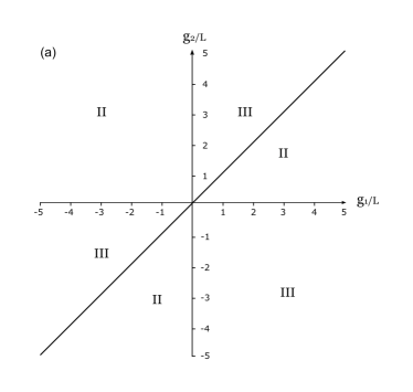
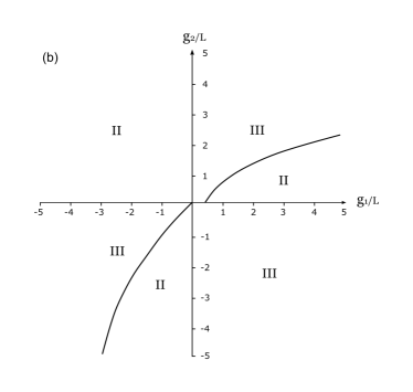
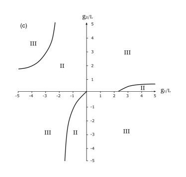
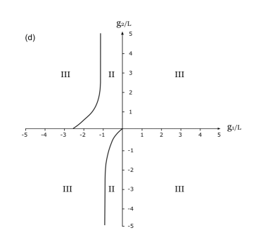
Figure 6: The $(g_{1},g_{2})$-phase portrait of the model at $\phi=0$, arbitrary fixed values of $L$ and for different values of chemical potential $\mu$. (a) The case $L\mu=0$. (b) The case $L\mu=0.2$. (c) The case $L\mu=0.4$. (d) The case $L\mu=0.6$. We use the same designations of the phases as in Fig. 1.

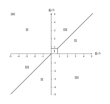
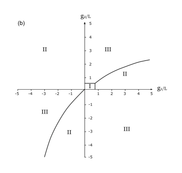
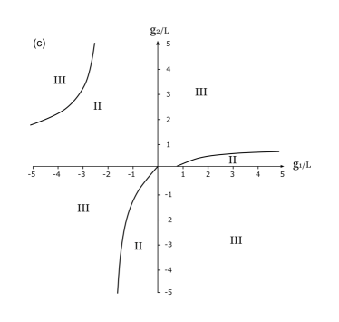
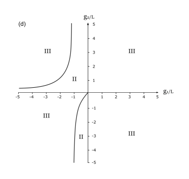
Figure 7: The $(g_{1},g_{2})$-phase portrait of the model at $\phi=1/12$, arbitrary fixed values of $L$ and for different values of chemical potential $\mu$. (a) The case $L\mu=0$. (b) The case $L\mu=0.2$. (c) The case $L\mu=0.4$. (d) The case $L\mu=0.6$. We use the same designations of the phases as in Fig. 1.

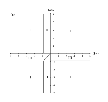
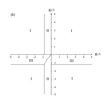
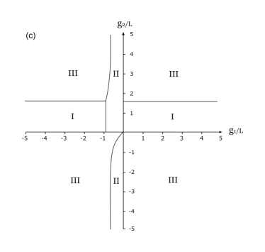
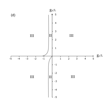
Figure 8: The $(g_{1},g_{2})$-phase portrait of the model at $\phi=1/3$, arbitrary fixed values of $L$ and for different values of chemical potential $\mu$. (a) The case $L\mu=0$. (b) The case $L\mu=0.6$. (c) The case $L\mu=1.2$. (d) The case $L\mu=1.8$. We use the same designations of the phases as in Fig. 1.

Figure 9: The behavior of the gap $\Delta_{0}$ vs $\mu$ at $g_{1}=-2L$, $g_{2}=-L$, $\phi=0$ and arbitrary fixed value of $L$. (In this case $M_{0}\equiv 0$ vs $\mu$).

Figure 10: The behavior of the gaps $\Delta_{0}$ and $M_{0}$ vs $\mu$ at $g_{1}=-L$, $g_{2}=-2L$, $\phi=0$ and arbitrary fixed value of $L$. The 1st order phase transition between CSB and SC phases occurs at $\mu_{c}\approx 0.49/L$.

In the previous Section we have pointed out that for some fixed points $(g_{1},g_{2})$ and $\mu=0$ there can appear in the model the reentering of the CSB or SC phases vs magnetic flux $\phi$. It is clear from Figs. 6-8 that the reentrance effect takes place for rather small fixed nonzero values of $\mu$ as well. Indeed, let us suppose that $L\mu=0.6$ and $(g_{1},g_{2})$ is fixed in such a way, e.g., that $g_{1}/L=g_{2}/L=-3$. Then at $\phi=0$ and $\phi=1/12$ we have in this point of the $(g_{1},g_{2})$-phase diagram the SC phase III (see Figs. 6d and 7d, correspondingly). However, at $\phi=1/3$ the symmetric phase I is already realized in this point (see Fig. 8b). Since all physical quantities of the model are periodical vs $\phi$, one can conclude that in the above mentioned fixed point $(g_{1},g_{2})$ and at $L\mu=0.6$ there are both periodical restoration of the initial symmetry and periodical reentering of the SC phase vs $\phi$. Since at rather large values of $\mu$ and for arbitrary values of the magnetic flux $\phi$ the $(g_{1},g_{2})$-phase structure of the model looks like the phase diagram of Fig. 8d with an extremely narrow phase II, it is necessary to note that the reentrance effect of the model disappears at sufficiently high values of the chemical potential.

VI Summary and conclusions

In this paper we have studied the competition between chiral and superconducting condensations in the framework of the (2+1)-dimensional 4FQFT model (1), when one of spatial coordinates is compactified and the two-dimensional space has $R^{1}\otimes S^{1}$ topology (the length of the circumference $S^{1}$ is $L$). We consider this $R^{1}\otimes S^{1}$ space as a cylinder embedded into the real flat three-dimensional space. In addition, we supposed that there is an external magnetic field flux $\Phi$ through a transverse section of the cylinder (as a result, the boundary conditions (24) are fulfilled, where $\phi=\Phi/\Phi_{0}$). The model describes interactions both in the fermion-antifermion (or chiral) and superconducting difermion (or Cooper pairing) channels with bare couplings $G_{1}$ and $G_{2}$, respectively. Moreover, it is chirally and $U(1)$ invariant (the last group corresponds to conservation of the fermion number or electric charge of the system). To avoid the ban on the spontaneous breaking of continuous symmetry in (2+1)-dimensional field theories, we considered the phase structure of our model in the leading order of the large-$N$ technique, i.e. in the limit $N\to\infty$, where $N$ is a number of fermion fields, as it was done in the (1+1)-dimensional analog of the model chodos ; abreu . The temperature is zero in our consideration.

The case $L=\infty$, $\mu=0$. First of all we have investigated the thermodynamic potential of the model in the flat two-dimensional space with trivial topology, i.e. at $L=\infty$, with zero chemical potential $\mu=0$. In this case the phase portrait is presented in Fig. 1 in terms of the renormalization group invariant finite coupling constants $g_{1}$ and $g_{2}$, defined in (15). Each point $(g_{1},g_{2})$ of this diagram corresponds to a definite phase. For example, at $g_{1,2}>0$, i.e. at sufficiently small values of the bare coupling constants $G_{1,2}$ (see the comment at the end of Section II.2), both the discrete $\gamma^{5}$ chiral and $U(1)$ symmetries are not violated, and the system is in the symmetric phase, etc.

The case $L\neq\infty$, $\mu=0$. In this case there are two qualitatively different situations depending on the value of the magnetic flux $\phi$. Indeed, if $0\leq\phi<1/6$, then the typical $(g_{1},g_{2})$-phase portrait of the model is presented in Fig. 2, but if $1/6<\phi<1/2$, then the typical phase portrait of the model is drawn in Fig. 3. In particular, it follows from Fig. 2 that at $\phi=0$ (in this case the quantity $g_{c}$ (33) is equal to zero) we have in the region $g_{1,2}>0$ spontaneous breaking of the chiral $\gamma^{5}$ or $U(1)$ symmetry (in contrast, if $L=\infty$ then initial symmetry remains intact in this region). So, the compactification of the space, i.e. at $L\neq\infty$, induces spontaneous breaking of the symmetry.

Note also that all physical quantities of the model are periodic functions vs magnetic flux $\phi$ (see, e.g., Figs. 4 and 5, where the behavior of the CSB and SC gaps are presented). It is clear from Fig. 5 that for some points of the $(g_{1},g_{2})$ plane an increasing magnetic flux $\phi$ is accompanied by periodical reentrance of the SC (or CSB) phase. We expect that this effect can be observed in condensed matter experiments. Such a response of physical systems on the action of external magnetic field perpendicular to a direction of compactified coordinate is contrasted with the case, when magnetic field is directed along the compactified coordinate. In the last case the reentrance effect is absent 45 .

Finally, it is necessary to note that at finite $L$ and $\mu=0$ there is a duality between chiral symmetry breaking and superconductivity (see the relation (34). It means that if at the point $(g_{1},g_{2})$ of a phase diagram the CSB phase (the SC phase) is realized, then at the point $(g_{2},g_{1})$ one should have the SC phase (the CSB phase). Just this property of the model is evident from the phase diagrams of Figs 2 and 3.

The case $L\neq\infty$, $\mu\neq 0$. The $(g_{2},g_{1})$-phase portraits of the model are presented in this case in Figs 6–8 for the following representative values of the magnetic flux, $\phi=0$, $\phi=1/12$ and $\phi=1/3$, correspondingly. Moreover, in each figure four phase diagrams are drawn for different values of the chemical potential $\mu$. For example, in Figs. 6 and 7 chemical potential takes such values that $L\mu=0$, $L\mu=0.2$, $L\mu=0.4$, and $L\mu=0.6$, respectively. Comparing at each fixed $\phi$ the phase diagrams corresponding to different values of $\mu$, it is possible to establish the following interesting property of the model: at each fixed point of the $(g_{1},g_{2})$ plane (such that $g_{2}\neq 0$) and fixed $L\neq\infty$ the growth of the chemical potential leads to appearing of superconductivity in the system. (The same property of the chemical potential in the framework of the model (1) was established earlier in our paper kzz at $L=\infty$ even at nonzero temperature.) In particular, it means that if at $\mu=0$ we have in the model a SC ground state, then at arbitrary values of $\mu>0$ the superconductivity persists in the system as well. Moreover, if at $\mu=0$ we have in the model CSB or symmetrical ground state, then there is a critical value $\mu_{c}>0$ of the chemical potential, such that at $\mu>\mu_{c}$ initial CSB or symmetrical ground state is destroyed and the superconductivity appears. In other words, if in the physical system of fermions described by Lagrangian (1) and located on a cylindrical surface, there is an arbitrary small attractive interaction in the fermion-fermion channel, then it is possible to generate in the system the SC phenomenon by increasing the chemical potential.

It is necessary to note that the reentrance of the CSB or SC phases vs $\phi$ is also possible in the model at rather small nonzero values of $\mu$. However, in this case the reentrance effect disappears at sufficiently high values of the chemical potential (see the discussion at the end of Sec. V).

Since the results of the paper are valid for arbitrary values of $L$, $0<L<\infty$, we hope that our investigations can shed new light on physical phenomena taking place in nanotubes as well. In particular, taking into account the remarks made in the footnote 4, it is possible to relate phase diagrams of Figs. 6 and 8 to physical processes in metallic and semiconducting carbon nanotubes (with zero external magnetic flux), correspondingly.

Appendix A Algebra of the $\gamma$-matrices in the case of SO(2,1) group

The two-dimensional irreducible representation of the 3-dimensional Lorentz group SO(2,1) is realized by the following $2\times 2$ $\tilde{\gamma}$-matrices:

$$\tilde{\gamma}^{0}=\sigma_{3}=\left(\begin{array}[]{cc}1&0\\ 0&-1\end{array}\right),\,\,\tilde{\gamma}^{1}=i\sigma_{1}=\left(\begin{array}[]{cc}0&i\\ i&0\end{array}\right),\,\,\tilde{\gamma}^{2}=i\sigma_{2}=\left(\begin{array}[]{cc}0&1\\ -1&0\end{array}\right),$$ (43)

acting on two-component Dirac spinors. They have the properties:

$$Tr(\tilde{\gamma}^{\mu}\tilde{\gamma}^{\nu})=2g^{\mu\nu};~{}~{}[\tilde{\gamma}^{\mu},\tilde{\gamma}^{\nu}]=-2i\varepsilon^{\mu\nu\alpha}\tilde{\gamma}_{\alpha};~{}~{}\tilde{\gamma}^{\mu}\tilde{\gamma}^{\nu}=-i\varepsilon^{\mu\nu\alpha}\tilde{\gamma}_{\alpha}+g^{\mu\nu},$$ (44)

where $g^{\mu\nu}=g_{\mu\nu}=diag(1,-1,-1),~{}\tilde{\gamma}_{\alpha}=g_{\alpha\beta}\tilde{\gamma}^{\beta},~{}\varepsilon^{012}=1$. There is also the relation:

$$Tr(\tilde{\gamma}^{\mu}\tilde{\gamma}^{\nu}\tilde{\gamma}^{\alpha})=-2i\varepsilon^{\mu\nu\alpha}.$$ (45)

Note that the definition of chiral symmetry is slightly unusual in three dimensions (spin is here a pseudoscalar rather than a (axial) vector). The formal reason is simply that there exists no other $2\times 2$ matrix anticommuting with the Dirac matrices $\tilde{\gamma}^{\nu}$ which would allow the introduction of a $\gamma^{5}$-matrix in the irreducible representation. The important concept of ’chiral’ symmetries and their breakdown by mass terms can nevertheless be realized also in the framework of (2+1)-dimensional quantum field theories by considering a four-component reducible representation for Dirac fields. In this case the Dirac spinors $\psi$ have the following form:

$$\psi(x)=\left(\begin{array}[]{cc}\tilde{\psi}_{1}(x)\\ \tilde{\psi}_{2}(x)\end{array}\right),$$ (48)

with $\tilde{\psi}_{1},\tilde{\psi}_{2}$ being two-component spinors. In the reducible four-dimensional spinor representation one deals with (4$\times$4) $\gamma$-matrices: $\gamma^{\mu}=diag(\tilde{\gamma}^{\mu},-\tilde{\gamma}^{\mu})$, where $\tilde{\gamma}^{\mu}$ are given in (43). One can easily show, that ($\mu,\nu=0,1,2$):

$$Tr(\gamma^{\mu}\gamma^{\nu})=4g^{\mu\nu};~{}~{}\gamma^{\mu}\gamma^{\nu}=\sigma^{\mu\nu}+g^{\mu\nu};~{}~{}$$

$$\sigma^{\mu\nu}=\frac{1}{2}[\gamma^{\mu},\gamma^{\nu}]=diag(-i\varepsilon^{\mu\nu\alpha}\tilde{\gamma}_{\alpha},-i\varepsilon^{\mu\nu\alpha}\tilde{\gamma}_{\alpha}).$$ (49)

In addition to the Dirac matrices $\gamma^{\mu}~{}~{}(\mu=0,1,2)$ there exist two other matrices $\gamma^{3}$, $\gamma^{5}$ which anticommute with all $\gamma^{\mu}~{}~{}(\mu=0,1,2)$ and with themselves

$$\gamma^{3}=\left(\begin{array}[]{cc}0~{},&I\\ I~{},&0\end{array}\right),\,\gamma^{5}=\gamma^{0}\gamma^{1}\gamma^{2}\gamma^{3}=i\left(\begin{array}[]{cc}0~{},&-I\\ I~{},&0\end{array}\right),\,\,$$ (54)

with $I$ being the unit $2\times 2$ matrix.

Appendix B Proper-time representation of the TDP (13)

Let us derive another expression for the unrenormalized TDP $V^{un}(M,\Delta)$ which is equivalent to (13), by using the Schwinger proper-time method. Here and in the next appendix we use the general relation

$$\sqrt{A}=\frac{1}{\sqrt{\pi}}\int_{0}^{\infty}\frac{ds}{s^{2}}\Big{(}1-e^{-s^{2}A}\Big{)},$$ (55)

where $A>0$ and an improper integral in the right-hand side is obviously a convergent one. Supposing that $A=A_{\pm}\equiv\sqrt{|\vec{p}|^{2}+(M\pm\Delta)^{2}}$, one can use the relation (55) in (13) and find

$$V^{un}(M,\Delta)=\frac{M^{2}}{4G_{1}}+\frac{\Delta^{2}}{4G_{2}} + \frac{1}{\sqrt{\pi}}\int\frac{d^{2}p}{(2\pi)^{2}}\Bigg{(}\sum_{\pm}\int_{0}^{\infty}\frac{ds}{s^{2}}e^{-s^{2}\left[p_{1}^{2}+p_{2}^{2}+(M\pm\Delta)^{2}\right]}~{}\Bigg{)},$$ (56)

where we have omitted an unessential infinite constant, which does not depend on dynamical variables $M$ and $\Delta$. (Due to this reason the proper-time integral in (56) and below, in (57), is divergent.) Integrating in (56) over $p_{1}$ and $p_{2}$, we obtain finally the following proper-time expression for the unrenormalized TDP (13):

$$V^{un}(M,\Delta)=\frac{M^{2}}{4G_{1}}+\frac{\Delta^{2}}{4G_{2}} + \frac{1}{4\pi^{3/2}}\sum_{\pm}\int_{0}^{\infty}\frac{ds}{s^{4}}e^{-s^{2}(M\pm\Delta)^{2}}.$$ (57)

Appendix C Derivation of expression (23) for the thermodynamic potential

Let us denote by $A_{n,\pm}$ the following expression:

$$A_{n,\pm}=p_{1}^{2}+\frac{4\pi^{2}(n+\phi)^{2}}{L^{2}}+(M\pm\Delta)^{2}.$$ (58)

Then the TDP (22) has the form:

$$V^{un}_{L\phi}(M,\Delta)=\frac{M^{2}}{4G_{1}}+\frac{\Delta^{2}}{4G_{2}} - \frac{1}{L}\int\frac{dp_{1}}{2\pi}\sum_{n=-\infty}^{\infty}\Bigg{(}\sum_{\pm}\sqrt{A_{n,\pm}}~{}\Bigg{)}.$$ (59)

To proceed, it is very convenient to use for square roots $\sqrt{A_{n,\pm}}$ in (59) the proper-time representation (55). Then, up to an infinite constant independent on dynamical variables $M$ and $\Delta$, we have

$$V^{un}_{L\phi}(M,\Delta)=\frac{M^{2}}{4G_{1}}+\frac{\Delta^{2}}{4G_{2}} + \frac{1}{L\sqrt{\pi}}\sum_{\pm}\int\frac{dp_{1}}{2\pi}\sum_{n=-\infty}^{\infty}\int_{0}^{\infty}\frac{ds}{s^{2}}e^{-s^{2}\left[p_{1}^{2}+(M\pm\Delta)^{2}+\frac{4\pi^{2}}{L^{2}}(n+\phi)^{2}\right]}.$$ (60)

First of all let us sum in (60) over $n$, taking into account there the well-known Poisson summation formula,

$$\sum_{n=-\infty}^{\infty}e^{-s^{2}\frac{4\pi^{2}}{L^{2}}(n+\phi)^{2}}=\frac{L}{2\pi}\frac{\sqrt{\pi}}{s}\sum_{n=-\infty}^{\infty}e^{-\frac{n^{2}L^{2}}{4s^{2}}}e^{i2\pi n\phi}=\frac{L}{2\pi}\frac{\sqrt{\pi}}{s}\biggl{\{}1+2\sum_{n=1}^{\infty}e^{-\frac{n^{2}L^{2}}{4s^{2}}}\cos(2\pi n\phi)\biggr{\}}.$$ (61)

Then, after integration in the obtained expression over $p_{1}$, we have

$$V^{un}_{L\phi}(M,\Delta)=V^{un}(M,\Delta)+\frac{1}{2\pi^{3/2}}\sum_{\pm}\sum_{n=1}^{\infty}\int_{0}^{\infty}\frac{ds}{s^{4}}e^{-s^{2}(M\pm\Delta)^{2}-\frac{n^{2}L^{2}}{4s^{2}}}\cos(2\pi n\phi),$$ (62)

where $V^{un}(M,\Delta)$ is the proper-time represented effective potential of the model in the vacuum (57). Taking into account the relation

$$\int\limits^{\infty}_{0}dxx^{\nu-1}e^{-\frac{a}{x}-bx}=2\left(\frac{a}{b}\right)^{\nu/2}K_{\nu}(2\sqrt{ab}),$$

it is possible to integrate in (62) over $s$,

$$V^{un}_{L\phi}(M,\Delta)=V^{un}(M,\Delta)+\frac{1}{2\pi^{3/2}}\sum_{\pm}\sum_{n=1}^{\infty}\left(\frac{2|M\pm\Delta|}{nL}\right)^{3/2}K_{-\frac{3}{2}}\Big{(}nL|M\pm\Delta|\Big{)}\cos(2\pi n\phi),$$ (63)

where $K_{\nu}(z)$ is the third order modified Bessel function, and

$$K_{-\frac{3}{2}}(z)=K_{\frac{3}{2}}(z)=-\sqrt{\frac{\pi z}{2}}\frac{d}{dz}\left(\frac{e^{-z}}{z}\right)=\sqrt{\frac{\pi z}{2}}e^{-z}\frac{z+1}{z^{2}}.$$ (64)

Using the relation (64) in (63), we obtain the expression (23) for the unrenormalized effective potential at $L\neq\infty$ and $\mu=0$.

References

- (1) D. Ebert and M.K. Volkov, Z. Phys. C 16, 205 (1983); D. Ebert, H. Reinhardt and M.K. Volkov, Prog. Part. Nucl. Phys. 33, 1 (1994).
- (2) M. Buballa, Phys. Rept. 407, 205 (2005); M. Buballa and S. Carignano, arXiv:1406.1367 [hep-ph].
- (3) E.J. Ferrer, V. de la Incera and C. Manuel, PoS JHW 2005, 022 (2006).
- (4) R. Gatto and M. Ruggieri, Lect. Notes Phys. 871, 87 (2013) [arXiv:1207.3190 [hep-ph]].
- (5) A.A. Andrianov, D. Espriu and X. Planells, Eur. Phys. J. C 73, 2294 (2013); Eur. Phys. J. C 74, 2776 (2014).
- (6) B. Hiller, A.A. Osipov, A.H. Blin and J. da Providencia, SIGMA 4, 024 (2008) [arXiv:0802.3193 [hep-ph]].
- (7) J.O. Andersen, W.R. Naylor and A. Tranberg, arXiv:1411.7176 [hep-ph].
- (8) D.J. Gross and A. Neveu, Phys. Rev. D 10, 3235 (1974).
- (9) A. Chodos and H. Minakata, Phys. Lett. A 191, 39 (1994); H. Caldas, J.L. Kneur, M.B. Pinto and R.O. Ramos, Phys. Rev. B 77, 205109 (2008).
- (10) A. Chodos, H. Minakata, F. Cooper, A. Singh, and W. Mao, Phys. Rev. D 61, 045011 (2000).
- (11) L.M. Abreu, A.P.C. Malbouisson and J.M.C. Malbouisson, Phys. Rev. D 83, 025001 (2011). Europhys. Lett. 90, 11001 (2010).
- (12) D. Ebert, T.G. Khunjua, K.G. Klimenko and V.C. Zhukovsky, Phys. Rev. D 90, 045021 (2014);
- (13) D. Ebert, K.G. Klimenko, A.V. Tyukov and V.C. Zhukovsky, Phys. Rev. D 78, 045008 (2008); D. Ebert, K.G. Klimenko, Phys. Rev. D80, 125013 (2009); D. Ebert, N.V. Gubina, K.G. Klimenko, S.G. Kurbanov and V.C. Zhukovsky, Phys. Rev. D 84, 025004 (2011).
- (14) N.V. Gubina, K.G. Klimenko, S.G. Kurbanov and V.C. Zhukovsky, Phys. Rev. D 86, 085011 (2012).
- (15) M. Thies, Phys. Rev. D 68, 047703 (2003); Phys. Rev. D 90, no. 10, 105017 (2014).
- (16) O. Schnetz, M. Thies and K. Urlichs, Annals Phys. 314, 425 (2004); G. Basar, G.V. Dunne and M. Thies, Phys. Rev. D 79, 105012 (2009); C. Boehmer and M. Thies, Phys. Rev. D 80, 125038 (2009).
- (17) G.W. Semenoff and L.C.R. Wijewardhana, Phys. Rev. Lett. 63, 2633 (1989); Phys. Rev. D 45, 1342 (1992).
- (18) B. Rosenstein, B.J. Warr and S.H. Park, Phys. Rep. 205, 59 (1991).
- (19) K.G. Klimenko, Z. Phys. C 37, 457 (1988); A.S. Vshivtsev, B.V. Magnitsky, V.C. Zhukovsky and K.G. Klimenko, Phys. Part. Nucl. 29, 523 (1998) [Fiz. Elem. Chast. Atom. Yadra 29, 1259 (1998)].
- (20) T. Inagaki, T. Kouno and T. Muta, Int. J. Mod. Phys. A 10, 2241 (1995).
- (21) T. Appelquist and M. Schwetz, Phys. Lett. B 491, 367 (2000); S.J. Hands, J.B. Kogut and C.G. Strouthos, Phys. Lett. B 515, 407 (2001); Phys. Rev. D 65, 114507 (2002).
- (22) D. Ebert, K. G. Klimenko and H. Toki, Phys. Rev. D 64, 014038 (2001); H. Kohyama, Phys. Rev. D 77, 045016 (2008); Phys. Rev. D 78, 014021 (2008).
- (23) J.-L. Kneur, M.B. Pinto, R.O. Ramos and E. Staudt, Phys. Rev. D 76, 045020 (2007); Phys. Lett. B 657, 136 (2007).
- (24) K.G. Klimenko, Z. Phys. C 54, 323 (1992); Theor. Math. Phys. 90, 1 (1992); V.P. Gusynin, V.A. Miransky and I.A. Shovkovy, Phys. Rev. Lett. 73, 3499 (1994); I.A. Shovkovy, Lect. Notes Phys. 871, 13 (2013); V.A. Miransky and I.A. Shovkovy, arXiv:1503.00732.
- (25) H. Gies and S. Lippoldt, Phys. Rev. D 87, 104026 (2013).
- (26) K.G. Klimenko, Z. Phys. C 50, 477 (1991); Mod. Phys. Lett. A 9, 1767 (1994).
- (27) A.S. Davydov, Phys. Rep. 190, 191 (1990); M. Rotter, M. Tegel and D. Johrendt, Phys. Rev. Lett. 101, 107006 (2008).
- (28) A.J. Niemi and G.W. Semenoff, Phys. Rev. Lett. 54, 873 (1985).
- (29) A.H. Castro Neto, F. Guinea, N.M.R. Peres, K.S. Novoselov and A.K. Geim, Rev. Mod. Phys. 81, 109 (2009).
- (30) G.W. Semenoff, I.A. Shovkovy and L.C.R. Wijewardhana, Mod. Phys. Lett. A 13, 1143 (1998).
- (31) H. Caldas and R.O. Ramos, Phys. Rev. B 80, 115428 (2009); J.L. Kneur, M.B. Pinto and R.O. Ramos, Phys. Rev. D 88, 045005 (2013); R.O. Ramos and P.H.A. Manso, Phys. Rev. D 87, 125014 (2013); K.G. Klimenko and R.N. Zhokhov, Phys. Rev. D 88, 105015 (2013).
- (32) B. Roy, Phys. Rev. B 84, 035458 (2011).
- (33) V.C. Zhukovsky, K.G. Klimenko, V.V. Khudyakov and D. Ebert, JETP Lett. 73, 121 (2001); V.C. Zhukovsky and K.G. Klimenko, Theor. Math. Phys. 134, 254 (2003); E.J. Ferrer, V.P. Gusynin and V. de la Incera, Mod. Phys. Lett. B 16, 107 (2002); Eur. Phys. J. B 33, 397 (2003).
- (34) E.C. Marino and L.H.C.M. Nunes, Nucl. Phys. B 741, 404 (2006); L.H.C.M. Nunes, R.L.S. Farias and E.C. Marino, Phys. Lett. A 376, 779 (2012).
- (35) K.G. Klimenko, R.N. Zhokhov and V.C. Zhukovsky, Phys. Rev. D 86, 105010 (2012); Mod. Phys. Lett. A 28, 1350096 (2013).
- (36) G. Cao, L. He and P. Zhuang, Phys. Rev. D 90, no. 5, 056005 (2014).
- (37) N.D. Mermin and H. Wagner, Phys. Rev. Lett. 17, 1133 (1966); S. Coleman, Commun. Math. Phys. 31, 259 (1973).
- (38) D. Ebert and K.G. Klimenko, Phys. Rev. D 82, 025018 (2010) [arXiv:1005.0699 [hep-ph]].
- (39) I.V. Krive and S.A. Naftlin, Nucl. Phys. B 364, 541 (1991); D.Y. Song, Phys. Rev. D 48, 3925 (1993); S. Huang and B. Schreiber, Nucl. Phys. B 426, 644 (1994).
- (40) A.V. Gamayun and E.V. Gorbar, Phys. Lett. B 610, 74 (2005).
- (41) V.C. Zhukovsky and P.B. Kolmakov, Moscow Univ. Phys. Bull. 68, 272 (2013) [Vestn. Mosk. Univ. 2013, no. 4, 8ñ14 (2013)].
- (42) T. Inagaki, T. Kouno and T. Muta, Int. J. Mod. Phys. A 10, 2241 (1995); S. Kanemura and H. T. Sato, Mod. Phys. Lett. A 11, 785 (1996); D.M. Gitman, S.D. Odintsov and Y.I. Shilnov, Phys. Rev. D 54, 2968 (1996). D.K. Kim and K.G. Klimenko, J. Phys. A 31, 5565 (1998).
- (43) A. Flachi, Phys. Rev. D 86, 104047 (2012); A. Flachi, Phys. Rev. Lett. 110, no. 6, 060401 (2013); A. Flachi and K. Fukushima, Phys. Rev. Lett. 113, no. 9, 091102 (2014).
- (44) T. Ando, J. Phys. Soc. Jpn., 74, 777 (2005).
- (45) E.J. Ferrer, V.P. Gusynin and V. de la Incera, Phys. Lett. B 455, 217 (1999).