Fast Estimation of the Median Covariation Matrix with Application to Online Robust Principal Components Analysis
Abstract
The geometric median covariation matrix is a robust multivariate indicator of dispersion which can be extended without any difficulty to functional data. We define estimators, based on recursive algorithms, that can be simply updated at each new observation and are able to deal rapidly with large samples of high dimensional data without being obliged to store all the data in memory. Asymptotic convergence properties of the recursive algorithms are studied under weak conditions. The computation of the principal components can also be performed online and this approach can be useful for online outlier detection. A simulation study clearly shows that this robust indicator is a competitive alternative to minimum covariance determinant when the dimension of the data is small and robust principal components analysis based on projection pursuit and spherical projections for high dimension data. An illustration on a large sample and high dimensional dataset consisting of individual TV audiences measured at a minute scale over a period of 24 hours confirms the interest of considering the robust principal components analysis based on the median covariation matrix. All studied algorithms are available in the R package Gmedian on CRAN.
Keywords. Averaging, Functional data, Geometric median, Online algorithms, Online principal components, Recursive robust estimation, Stochastic gradient, Weiszfeld’s algorithm.
1 Introduction
Principal Components Analysis is one of the most useful statistical tool to extract information by reducing the dimension when one has to analyze large samples of multivariate or functional data (see e.g. Jolliffe, (2002) or Ramsay and Silverman, (2005)). When both the dimension and the sample size are large, outlying observations may be difficult to detect automatically. Principal components, which are derived from the spectral analysis of the covariance matrix, can be very sensitive to outliers (see Devlin et al., (1981)) and many robust procedures for principal components analysis have been considered in the literature (see Hubert et al., (2008), Huber and Ronchetti, (2009) and Maronna et al., (2006)).
The most popular approaches are probably the minimum covariance determinant estimator (see Rousseeuw and van Driessen, (1999)) and the robust projection pursuit (see Croux and Ruiz-Gazen, (2005) and Croux et al., (2007)). Robust PCA based on projection pursuit has been extended to deal with functional data in Hyndman and Ullah, (2007) and Bali et al., (2011). Adopting another point of view, robust modifications of the covariance matrix, based on projection of the data onto the unit sphere, have been proposed in Locantore et al., (1999) (see also Gervini, (2008) and Taskinen et al., (2012)).
We consider in this work another robust way of measuring association between variables, that can be extended directly to functional data. It is based on the notion of median covariation matrix (MCM) which is defined as the minimizer of an expected loss criterion based on the Hilbert-Schmidt norm (see Kraus and Panaretos, (2012) for a first definition in a more general -estimation setting). It can be seen as a geometric median (see Kemperman, (1987) or Möttönen et al., (2010)) in the particular Hilbert spaces of square matrices (or operators for functional data) equipped with the Frobenius (or Hilbert-Schmidt) norm. The MCM is non negative and unique under weak conditions. As shown in Kraus and Panaretos, (2012) it also has the same eigenspace as the usual covariance matrix when the distribution of the data is symmetric and the second order moment is finite. Being a spatial median in a particular Hilbert space of matrices, the MCM is also a robust indicator of central location, among the covariance matrices, which has a 50 % breakdown point (see Kemperman, (1987) or Maronna et al., (2006)) as well as a bounded gross sensitivity error (see Cardot et al., (2013)).
The aim of this work is twofold. It provides efficient recursive estimation algorithms of the MCM that are able to deal with large samples of high dimensional data. By this recursive property, these algorithms can naturally deal with data that are observed sequentially and provide a natural update of the estimators at each new observation. Another advantage compared to classical approaches is that such recursive algorithms will not require to store all the data. Secondly, this work also aims at highlighting the interest of considering the median covariation matrix to perform principal components analysis of high dimensional contaminated data.
Different algorithms can be considered to get effective estimators of the MCM. When the dimension of the data is not too high and the sample size is not too large, Weiszfeld’s algorithm (see Weiszfeld, (1937) and Vardi and Zhang, (2000)) can be directly used to estimate effectively both the geometric median and the median covariation matrix. When both the dimension and the sample size are large this static algorithm which requires to store all the data may be inappropriate and ineffective. We show how the algorithm developed by Cardot et al., (2013) for the geometric median in Hilbert spaces can be adapted to estimate recursively and simultaneously the median as well as the median covariation matrix. Then an averaging step (Polyak and Juditsky, (1992)) of the two initial recursive estimators of the median and the MCM permits to improve the accuracy of the initial stochastic gradient algorithms. A simple modification of the stochastic gradient algorithm is proposed in order to ensure that the median covariance estimator is non negative. We also explain how the eigenelements of the estimator of the MCM can be updated online without being obliged to perform a new spectral decomposition at each new observation.
The paper is organized as follows. The median covariation matrix as well as the recursive estimators are defined in Section 2. In Section 3, almost sure and quadratic mean consistency results are given for variables taking values in general separable Hilbert spaces. The proofs, which are based on new induction steps compared to Cardot et al., (2013), allow to get better convergence rates in quadratic mean even if this new framework is much more complicated because two averaged non linear algorithms are running simultaneously. One can also note that the techniques generally employed to deal with two time scale Robbins Monro algorithms (see Mokkadem and Pelletier, (2006) for the multivariate case) require assumptions on the rest of the Taylor expansion and the finite dimension of the data that are too restrictive in our framework. In Section 4, a comparison with some classic robust PCA techniques is made on simulated data. The interest of considering the MCM is also highlighted on the analysis of individual TV audiences, a large sample of high dimensional data which, because of its dimension, can not be analyzed in a reasonable time with classical robust PCA approaches. The main parts of the proofs are described in Section 5. Perspectives for future research are discussed in Section 6. Some technical parts of the proofs as well as a description of Weiszfeld’s algorithm in our context are gathered in an Appendix.
2 Population point of view and recursive estimators
Let be a separable Hilbert space (for example or , for some closed interval ). We denote by its inner product and by the associated norm.
We consider a random variable that takes values in and define its center as follows:
| (1) |
The solution is often called the geometric median of . It is uniquely defined under broad assumptions on the distribution of (see Kemperman, (1987)) which can be expressed as follows.
Assumption 1.
There exist two linearly independent unit vectors , such that
If the distribution of is symmetric around zero and if admits a first moment that is finite then the geometric median is equal to the expectation of , . Note however that the general definition (1) does not require to assume that the first order moment of is finite since .
2.1 The (geometric) median covariation matrix (MCM)
We now consider the special vector space, denoted by , of matrices when , or for general separable Hilbert spaces , the vector space of linear operators mapping . Denoting by an orthonormal basis in , the vector space equipped with the following inner product:
| (2) |
is also a separable Hilbert space. In , we have equivalently
| (3) |
where is the transpose matrix of . The induced norm is the well known Frobenius norm (also called Hilbert-Schmidt norm) and is denoted by
When has finite second order moments, with expectation , the covariance matrix of , can be defined as the minimum argument, over all the elements belonging to , of the functional ,
Note that in general Hilbert spaces with inner product , operator should be understood as the operator . The MCM is obtained by removing the squares in previous function in order to get a more robust indicator of "covariation". For , define by
| (4) |
The median covariation matrix, denoted by , is defined as the minimizer of over all elements . The second term at the right-hand side of (4) prevents from having to introduce hypotheses on the existence of the moments of . Introducing the random variable that takes values in , the MCM is unique provided that the support of is not concentrated on a line and Assumption 1 can be rephrased as follows in ,
Assumption 2.
There exist two linearly independent unit vectors , such that
We can remark that Assumption 1 and Assumption 2 are strongly connected. Indeed, if Assumption 1 holds, then for . Consider the rank one matrices and , we have which has a strictly positive variance when the distribution of has no atom. More generally unless there is a scalar such that (assuming also that ).
Furthermore it can be deduced easily that the MCM, which is a geometric median in the particular Hilbert spaces of Hilbert-Schmidt operators, is a robust indicator with a 50% breakdown point (see Kemperman, (1987)) and a bounded sensitive gross error (see Cardot et al., (2013)).
We also assume that
Assumption 3.
There is a constant such that for all and all
This assumption implicitly forces the distribution of to have no atoms. It is more "likely" to be satisfied when the dimension of the data is large (see Chaudhuri, (1992) and Cardot et al., (2013) for a discussion). Note that it could be weakened as in Cardot et al., (2013) by allowing points, necessarily different from the MCM , to have strictly positive masses. Considering the particular case , Assumption 3(a) implies that for all ,
| (5) |
and this is not restrictive when the dimension of is equal or larger than 3.
Under Assumption 3(a), the functional is twice Fréchet differentiable, with gradient
| (6) |
and Hessian operator, ,
| (7) |
where , is the identity operator on and for any elements and belonging to .
Furthermore, is also defined as the unique zero of the non linear equation:
| (8) |
Remarking that previous equality can be rewritten as follows,
| (9) |
it is clear that is a bounded, symmetric and non negative operator in .
As stated in Proposition 2 of Kraus and Panaretos, (2012), operator has an important stability property when the distribution of is symmetric, with finite second moment, i.e . Indeed, the covariance operator of , , which is well defined in this case, and share the same eigenvectors: if is an eigenvector of with corresponding eigenvalue , then , for some non negative value . This important result means that for Gaussian and more generally symmetric distribution (with finite second order moments), the covariance operator and the median covariation operator have the same eigenspaces. Note that it is also conjectured in Kraus and Panaretos, (2012) that the order of the eigenfunctions is also the same.
2.2 Efficient recursive algorithms
We suppose now that we have i.i.d. copies of random variables with the same law as .
For simplicity, we temporarily suppose that the median of is known. We consider a sequence of (learning) weights , with and and we define the recursive estimation procedure as follows
| (10) | ||||
| (11) |
This algorithm can be seen as a particular case of the averaged stochastic gradient algorithm studied in Cardot et al., (2013). Indeed, the first recursive algorithm (10) is a stochastic gradient algorithm,
where is the -algebra generated by whereas the final estimator is obtained by averaging the past values of the first algorithm. The averaging step (see Polyak and Juditsky, (1992)), i.e. the computation of the arithmetical mean of the past values of a slowly convergent estimator (see Proposition 3.4 below), permits to obtain a new and efficient estimator converging at a parametric rate, with the same asymptotic variance as the empirical risk minimizer (see Theorem 3.1 below).
In most of the cases the value of is unknown so that it also required to estimate the median. To build an estimator of , it is possible to estimate simultaneously and by considering two averaged stochastic gradient algorithms that are running simultaneously. For ,
| (12) | ||||
| (13) | ||||
| (14) |
where the averaged recursive estimator of the median is controlled by a sequence of descent steps . The learning rates are generally chosen as follows, , where the tuning constants satisfy and .
Note that by construction, even if is non negative, may not be a non negative matrix when the learning steps do not satisfy
Projecting onto the closed convex cone of non negative operators would require to compute the eigenvalues of which is time consuming in high dimension even if is a rank one perturbation to (see Cardot and Degras, (2015)). We consider the following simple approximation to this projection which consists in replacing in (13) the descent step by a thresholded one,
| (15) |
which ensures that remains non negative when is non negative. The use of these modified steps and an initialization of the recursive algorithm (13) with a non negative matrix (for example ) ensure that for all , and are non negative.
2.3 Online estimation of the principal components
It is also possible to approximate recursively the eigenvectors (unique up to sign) of associated to the largest eigenvalues without being obliged to perform a spectral decomposition of at each new observation. Many recursive strategies can be employed (see Cardot and Degras, (2015) for a review on various recursive estimation procedures of the eigenelements of a covariance matrix). Because of its simplicity and its accuracy, we consider the following one:
| (16) |
combined with an orthogonalization by deflation of . This recursive algorithm is based on ideas developed by Weng et al., (2003) that are related to the power method for extracting eigenvectors. If we assume that the first eigenvalues are distinct, the estimated eigenvectors , which are uniquely determined up to sign change, tend to
Once the eigenvectors are computed, it is possible to compute the principal components as well as indices of outlyingness for each new observation (see Hubert et al., (2008) for a review of outliers detection with multivariate approaches).
2.4 Practical issues, complexity and memory
The recursive algorithms (13) and (14) require each elementary operations at each update. With the additional online estimation given in (16) of the eigenvectors associated to the largest eigenvalues, additional operations are required. The orthogonalization procedure only requires elementary operations.
Note that the use of classical Newton-Raphson algorithms for estimating the MCM (see Fritz et al., (2012)) can not be envisaged for high dimensional data since the computation or the approximation of the Hessian matrix would require elementary operations. The well known and fast Weiszfeld’s algorithm requires elementary operations for each sample with size . However, the estimation cannot be updated automatically if the data arrive sequentially. Another drawback compared to the recursive algorithms studied in this paper is that all the data must be stored in memory, which is of order elements whereas the recursive technique require an amount of memory of order .
The performances of the recursive algorithms depend on the values of tuning parameters , and . The value of parameter is often chosen to be or . Previous empirical studies (see Cardot et al., (2013) and Cardot et al., (2010)) have shown that, thanks to the averaging step, estimator performs well and is not too sensitive to the choice of , provided that the value of is not too small. An intuitive explanation could be that here the recursive process is in some sense "self-normalized" since the deviations at each iteration in (10) have unit norm and finding some universal values for is possible. Usual values for and are in the interval . When is fixed, this averaged recursive algorithm is about 30 times faster than the Weiszfeld’s approach (see Cardot et al., (2013)).
3 Asymptotic properties
When is known, can be seen as an averaged stochastic gradient estimator of the geometric median in a particular Hilbert space and the asymptotic weak convergence of such estimator has been studied in Cardot et al., (2013). They have shown that:
Theorem 3.1.
(Cardot et al., (2013), Theorem 3.4).
If assumptions 1-3(a) hold, then as tends to infinity,
where stands for convergence in distribution and is the limiting covariance operator, with
As explained in Cardot et al., (2013), the estimator is efficient in the sense that it has the same asymptotic distribution as the empirical risk minimizer related to (see for the derivation of its asymptotic normality in Möttönen et al., (2010) in the multivariate case and Chakraborty and Chaudhuri, (2014) in a more general functional framework).
Using the delta method for weak convergence in Hilbert spaces (see Dauxois et al., (1982) or Cupidon et al., (2007)), one can deduce, from Theorem 3.1, the asymptotic normality of the estimated eigenvectors of . It can also be proven (see Godichon-Baggioni, (2016)), under Assumptions 1-3, that there is a positive constant such that for all ,
Note finally that non asymptotic bounds for the deviation of around can be derived readily with the general results given in Cardot et al., (2016).
The more realistic case in which must also be estimated is more complicated because depends on which is also estimated recursively with the same data. We first state the strong consistency of the estimators and .
Theorem 3.2.
If assumptions 1-3(b) hold, we have
and
The obtention of the rate convergence of the averaged recursive algorithm relies on a fine control of the asymptotic behavior of the Robbins-Monro algorithms, as stated in the following proposition.
Theorem 3.3.
If assumptions 1-3(b) hold, there is a positive constant , and for all , there is a positive constant such that for all ,
The obtention of an upper bound for the rate of convergence at the order four of the Robbins-Monro algorithm is crucial in the proofs. Furthermore, the following proposition ensures that the exhibited rate in quadratic mean is the optimal one.
Proposition 3.4.
Under assumptions 1-3(b), there is a positive constant such that for all ,
Finally, the following theorem is the most important theoretical result of this work. It shows that, in spite of the fact that it only considers the observed data one by one, the averaged recursive estimation procedure gives an estimator which has a classical parametric rate of convergence in the Hilbert-Schmidt norm.
Theorem 3.5.
Under Assumptions 1-3(b), there is a positive constant such that for all ,
4 An illustration on simulated and real data
A small comparison with other classical robust PCA techniques is performed in this section considering data in relatively high dimension but samples with moderate sizes. This permits to compare our approach with classical robust PCA techniques, which are generally not designed to deal with large samples of high dimensional data. In our comparison, we have employed the following well known robust techniques: robust projection pursuit (see Croux and Ruiz-Gazen, (2005) and Croux et al., (2007)), minimum covariance determinant (MCD, see Rousseeuw and van Driessen, (1999)) and spherical PCA (see Locantore et al., (1999)). The computations were made in the R language (R Development Core Team, (2010)), with the help of packages pcaPP and rrcov. For reproductible research, our codes for computing the MCM have been posted on CRAN in the Gmedian package. We will denote by MCM(R) the recursive estimator defined in (14) and MCM(R+) its non negative modification whose learning weights are defined in (15).
If the size of the data is not too large, an effective way for estimating is to employ Weiszfeld’s algorithm (see Weiszfeld, (1937) and Vardi and Zhang, (2000) as well the Supplementary file for a description of the algorithms in our particular situation). The estimate obtained thanks to Weiszfeld’s algorithm is denoted by MCM(W) in the following. Note that other optimization algorithms which may be preferred in small dimension (see Fritz et al., (2012)) have not been considered here since they would require the computation of the Hessian matrix, whose size is , and this would lead to much slower algorithms. Note finally that all these alternative algorithms do not admit a natural updating scheme when the data arrive sequentially so that they should be completely ran again at each new observation.
4.1 Simulation protocol
Independent realizations of a random variable are drawn, where
| (17) |
is a mixture of two distributions and and are independent random variables. The random vector has a centered Gaussian distribution in with covariance matrix and can be thought as a discretized version of a Brownian sample path in . The multivariate contamination comes from , with different rates of contamination controlled by the Bernoulli variable , independent from and , with and . Three different scenarios (see Figure 1) are considered for the distribution of :
-
•
The elements of vector are independent realizations of a Student distribution with one degree of freedom. This means that the first moment of is not defined when .
-
•
The elements of vector are independent realizations of a Student distribution with two degrees of freedom. This means that the second moment of is not defined when .
-
•
The vector is distributed as a "reverse time" Brownian motion. It has a Gaussian centered distribution, with covariance matrix . The covariance matrix of is .

For the averaged recursive algorithms, we have considered tuning coefficients and a speed rate of . Note that the values of these tuning parameters have not been particularly optimised. We have noted that the simulation results were very stable, and did not depend much on the value of and for .
The estimation error of the eigenspaces associated to the largest eigenvalues is evaluated by considering the squared Frobenius norm between the associated orthogonal projectors. Denoting by the orthogonal projector onto the space generated by the eigenvectors of the covariance matrix associated to the largest eigenvalues and by an estimation, we consider the following loss criterion,
| (18) |
Note that we always have and means that the eigenspaces generated by the true and the estimated eigenvectors are orthogonal.
4.2 Comparison with classical robust PCA techniques


We first compare the performances of the two estimators of the MCM based on the Weiszfeld’s algorithm and the recursive algorithms (see (14)) with more classical robust PCA techniques.
We generated samples of with size and dimension , over 500 replications. Different levels of contamination are considered : . For both dimensions and , the first eigenvalue of the covariance matrix of represents about 81 % of the total variance, and the second one about 9 %.
| PCA | MCD | MCM(W) | MCM(R+) | MCM(R) | SphPCA | PP | |
| d=50 | 0.0156 | 0.0199 | 0.0208 | 0.0211 | 0.0243 | 0.0287 | 0.0955 |
| d=200 | 0.0148 | - | 0.0200 | 0.0209 | 0.0246 | 0.0275 | 0.0895 |
The median errors of estimation of the eigenspace generated by the first two eigenvectors (), according to criterion (18), are given in Table 1 for non contaminated data (). The distribution of the estimation error is drawn for the different approaches in Figure 2 when the dimension is not large (). As expected, the "Oracle", which is the classical PCA in this situation, provides the best estimations of the eigenspaces. Then, the MCD and the median covariation matrix, estimated by the Weiszfeld algorithm or the modified MCM(R+) recursive estimator, behave well and similarly. Note that when the dimension gets larger, the MCD cannot be used anymore and the MCM is the more effective robust estimator of the eigenspaces.
When the data are contaminated, the median errors of estimation of the eigenspace generated by the first two eigenvectors (), according to criterion (18), are given in Table 2. In Figure 3, the distribution of the estimation error is drawn for the different approaches.
| 1 df | 2 df | inv. B. | 1 df | 2 df | inv. B. | ||
|---|---|---|---|---|---|---|---|
| Method | d = 50 | d = 200 | |||||
| 2% | PCA | 3.13 | 1.04 | 0.698 | 3.95 | 1.87 | 0.731 |
| PP | 0.086 | 0.097 | 0.090 | 0.085 | 0.094 | 0.084 | |
| MCD | 0.022 | 0.021 | 0.021 | – | – | – | |
| Sph. PCA | 0.028 | 0.029 | 0.027 | 0.027 | 0.030 | 0.028 | |
| MCM (Weiszfeld) | 0.021 | 0.021 | 0.021 | 0.021 | 0.022 | 0.022 | |
| MCM (R+) | 0.022 | 0.022 | 0.024 | 0.023 | 0.023 | 0.025 | |
| MCM (R) | 0.026 | 0.025 | 0.027 | 0.026 | 0.027 | 0.028 | |
| 5% | PCA | 3.82 | 1.91 | 0.862 | 3.96 | 1.98 | 0.910 |
| PP | 0.090 | 0.103 | 0.093 | 0.089 | 0.098 | 0.087 | |
| MCD | 0.022 | 0.023 | 0.021 | – | – | – | |
| Sph. PCA | 0.029 | 0.031 | 0.033 | 0.029 | 0.031 | 0.034 | |
| MCM (Weiszfeld) | 0.023 | 0.023 | 0.028 | 0.022 | 0.023 | 0.030 | |
| MCM (R+) | 0.025 | 0.024 | 0.035 | 0.024 | 0.024 | 0.039 | |
| MCM (R) | 0.029 | 0.027 | 0.037 | 0.028 | 0.028 | 0.040 | |
| 10% | PCA | 3.83 | 1.96 | 1.03 | 3.96 | 1.99 | 1.10 |
| PP | 0.107 | 0.108 | 0.099 | 0.088 | 0.101 | 0.097 | |
| MCD | 0.023 | 0.022 | 0.023 | – | – | – | |
| Sph. PCA | 0.033 | 0.033 | 0.054 | 0.031 | 0.033 | 0.057 | |
| MCM (Weiszfeld) | 0.025 | 0.026 | 0.059 | 0.023 | 0.024 | 0.056 | |
| MCM (R+) | 0.030 | 0.027 | 0.089 | 0.027 | 0.027 | 0.086 | |
| MCM (R) | 0.035 | 0.032 | 0.088 | 0.032 | 0.031 | 0.086 | |
| 20% | PCA | 3.84 | 2.02 | 1.19 | 3.96 | 2.01 | 1.25 |
| PP | 0.110 | 0.135 | 0.138 | 0.091 | 0.122 | 0.137 | |
| MCD | 0.025 | 0.026 | 0.026 | – | – | – | |
| Sph. PCA | 0.037 | 0.038 | 0.140 | 0.034 | 0.037 | 0.150 | |
| MCM (Weiszfeld) | 0.030 | 0.030 | 0.174 | 0.026 | 0.028 | 0.181 | |
| MCM (R+) | 0.044 | 0.036 | 0.255 | 0.038 | 0.032 | 0.256 | |
| MCM (R) | 0.050 | 0.041 | 0.251 | 0.042 | 0.037 | 0.256 | |
We can make the following remarks. At first note that even when the level of contamination is small (2% and 5%), the performances of classical PCA are strongly affected by the presence of outlying values in such (large) dimensions. When , the MCD algorithm and the MCM estimation provide the best estimations of the original two dimensional eigenspace, whereas when gets larger (), the MCD estimator can not be used anymore (by construction) and the MCM estimators, obtained with Weiszfeld’s and the non negative recursive algorithm, remain the most accurate. We can also remark that the recursive MCM algorithms, which are designed to deal with very large samples, performs well even for such moderate sample sizes (see also Figure 3). The modification of the descent step suggested in (15), which corresponds to estimator MCM(R+), permits to improve the accuracy the initial MCM estimator, specially when the noise level is not small. The performances of the spherical PCA are slightly less accurate whereas the median error of the robust PP is always the largest among the robust estimators. When, the contamination is highly structured temporally and the level of contamination is not small (contamination by a reverse time Brownian motion, with ), the behavior of the MCM is different from the other robust estimators and, with our criterion, it can appear as less effective. However, one can think that we are in presence of two different populations with completely different multivariate correlation structure and the MCD completely ignores that part of the data, which is not necessarily a better behavior.
4.3 Online estimation of the principal components
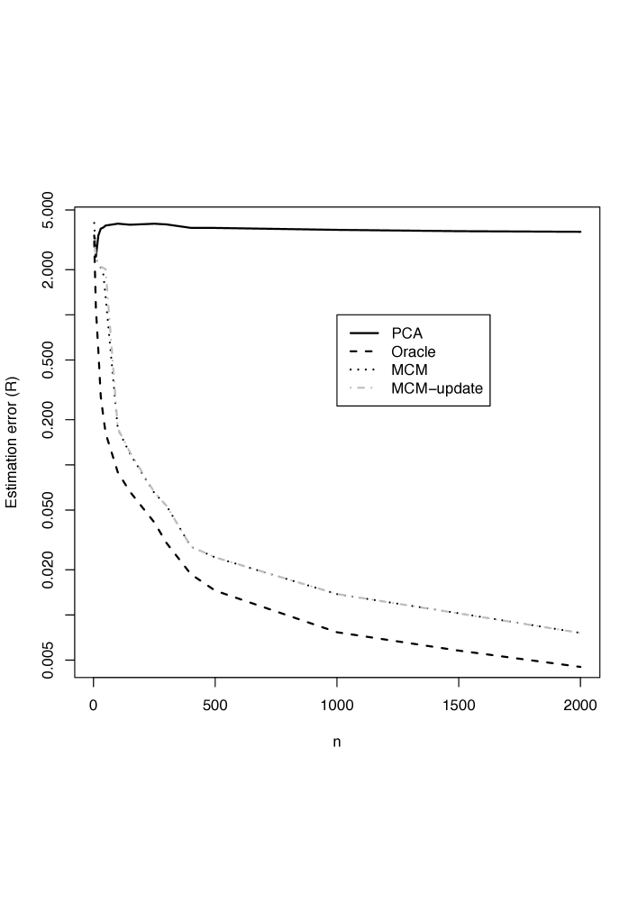
We now consider an experiment in high dimension, , and evaluate the ability of the recursive algorithms defined in (16) to estimate recursively the eigenvectors of associated to the largest eigenvalues. Note that due to the high dimension of the data and limited computation time, we only make comparison of the recursive robust techniques with the classical PCA. For this we generate growing samples and compute, for each sample size the approximation error of the different (fast) strategies to the true eigenspace generated by the eigenvectors associated to the largest eigenvalues of .
We have drawn in Figure 4, the evolution of the mean (over 100 replications) approximation error , for a dimension , as a function of the sample size for samples contaminated by a 2 degrees of freedom Student distribution with a rate . An important fact is that the recursive algorithm which approximates recursively the eigenelements behaves very well and we can see nearly no difference between the spectral decomposition of (denoted by MCM in Figure 4) and the estimates produced with the sequential algorithm (16) for sample sizes larger than a few hundreds. We can also note that the error made by the classical PCA is always very high and does not decrease with the sample size.
4.4 Robust PCA of TV audience
The last example is a high dimension and large sample case. Individual TV audiences are measured, by the French company Médiamétrie, every minutes for a panel of people over a period of 24 hours, (see Cardot et al., (2012) for a more detailed presentation of the data). With a classical PCA, the first eigenspace represents 24.4% of the total variability, whereas the second one reproduces 13.5% of the total variance, the third one 9.64% and the fourth one 6.79%. Thus, more than 54% of the variability of the data can be captured in a four dimensional space. Taking account of the large dimension of the data, these values indicate a high temporal correlation.
Because of the large dimension of the data, the Weiszfeld’s algorithm as well as the other robust PCA techniques can not be used anymore in a reasonable time with a personal computer. The MCM has been computed thanks to the recursive algorithm given in (14) in approximately 3 minutes on a laptop in the R language (without any specific C routine).
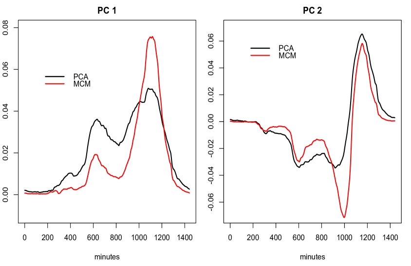
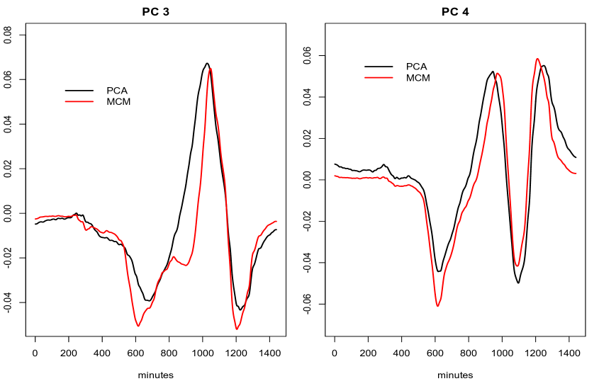
As seen in Figure 5, the first two eigenvectors obtained by a classical PCA and the robust PCA based on the MCM are rather different. This is confirmed by the relatively large distance between the two corresponding eigenspaces, . The first robust eigenvector puts the stress on the time period comprised between 1000 minutes and 1200 minutes whereas the first non robust eigenvector focuses, with a smaller intensity, on a larger period of time comprised between 600 and 1200 minutes. The second robust eigenvector differentiates between people watching TV during the period between 890 and 1050 minutes (negative value of the second principal component) and people watching TV between minutes 1090 and 1220 (positive value of the second principal component). Rather surprisingly, the third and fourth eigenvectors of the non robust and robust covariance matrices look quite similar (see Figure 6).
5 Proofs
We give in this Section the proofs of Theorems 3.2, 3.3 and 3.5. These proofs rely on several technical Lemmas whose proofs are given in the Supplementary file.
5.1 Proof of Theorem 3.2
Let us recall the Robbins-Monro algorithm, defined recursively by
with . Since , we have . Thus , is a sequence of martingale differences adapted to the filtration . Indeed, . The algorithm can be written as follows
Moreover, it can be considered as a stochastic gradient algorithm because it can be decomposed as follows:
| (19) |
with . Finally, linearizing the gradient,
| (20) |
with
The following lemma gives upper bounds of these remainder terms. Its proof is given in the Supplementary file.
Lemma 5.1.
Under assumptions 1-3(b), we can bound the three remainder terms. First,
| (21) |
In the same way, for all ,
| (22) |
Finally, for all ,
| (23) |
We deduce from decomposition (33) that for all ,
Note that for all and we have . Furthermore, and . Using the fact that is a sequence of martingale differences adapted to the filtration ,
Let , with , we have
| (24) | ||||
Moreover, applying Lemma 5.1 and Theorem 5.1 in Godichon-Baggioni, (2016), we get for all positive constant ,
Thus, since , the Robbins-Siegmund Theorem (see Duflo, (1997) for instance) ensures that converges almost surely to a finite random variable and
Furthermore, by induction, inequality (24) becomes
Since , applying Theorem 4.2 in Godichon-Baggioni, (2016) and Lemma 6.1, there is a positive constant such that
Thus, there is a positive constant such that for all , . Since converges almost surely to , one can conclude the proof of the almost sure consistency of with the same arguments as in the proof of Theorem 3.1 in Cardot et al., (2013) and the convexity properties given in the Section B of the supplementary file.
Finally, the almost sure consistency of is obtained by a direct application of Topelitz’s lemma (see e.g. Lemma 2.2.13 in Duflo, (1997)).
5.2 Proof of Theorem 3.3
The proof of Theorem 3.3 relies on properties of the -th moments of for all given in the following three Lemmas. These properties enable us, with the application of Markov’s inequality, to control the probability of the deviations of the Robbins Monro algorithm from .
Lemma 5.2.
Under assumptions 1-3(b), for all integer , there is a positive constant such that for all ,
Lemma 5.3.
Under assumptions 1-3(b), there are positive constants such that for all ,
where is the integer part of the real number .
Lemma 5.4.
Under assumptions 1-3(b), for all integer , there are a rank and positive constants such that for all ,
We can now prove Theorem 3.3.
Let us choose an integer such that . Thus, , and applying Lemma 5.4, there are positive constants and a rank such that for all ,
| (25) |
Let us now choose and such that . Note that . One can check that there is a rank such that for all ,
With the help of a strong induction, we are going to prove the announced results, that is to say that there are positive constants such that and (with defined in Lemma 5.3), such that for all ,
First, let us choose and such that
Thus, for all ,
We suppose from now that and that previous inequalities are verified for all . Applying Lemma 5.2 and by induction,
Since and since , factorizing by ,
By definition of ,
| (26) |
In the same way, applying Lemma 5.4 and by induction,
Since , factorizing by ,
By definition of ,
| (27) |
which concludes the induction and the proof.
5.3 Proof of Theorem 3.5
In order to prove Theorem 3.5, we first recall the following Lemma.
Lemma 5.5 (Godichon-Baggioni, (2016)).
Let be random variables taking values in a normed vector space such that for all positive constant and for all , . Then, for all real numbers and for all integer , we have
| (28) |
We can now prove Theorem 3.5. Let us rewrite decomposition (34) as follows
| (29) |
with . As in Pelletier, (2000), we sum these equalities, apply Abel’s transform and divide by to get
We now bound the quadratic mean of each term at the right-hand side of previous equality. First, we have . Applying Theorem 3.3,
Moreover, since , the application of Lemma 5.5 and Theorem 3.3 gives
since . In the same way, since , applying Lemma 5.5 and Theorem 3.3 with ,
Moreover, let . Since , and since there is a positive constant such that for all , ,
Since with , Cauchy-Schwarz’s inequality and Lemma 5.5 give
Applying Theorem 4.2 in Godichon-Baggioni, (2016) and Theorem 3.3,
since . Finally, one can easily check that , and since is a sequence of martingale differences adapted to the filtration ,
Thus, there is a positive constant such that for all ,
Let be the smallest eigenvalue of . We have, with Proposition B.1 in the supplementary file, that and the announced result is proven,
6 Concluding remarks
The simulation study and the illustration on real data indicate that performing robust principal components analysis via the median covariation matrix, which can bring new information compared to classical PCA, is an interesting alternative to more classical robust principal components analysis techniques. The use of recursive algorithms permits to perform robust PCA on very large datasets, in which outlying observations may be hard to detect. Another interest of the use of such sequential algorithms is that estimation of the median covariation matrix as well as the principal components can be performed online with automatic update at each new observation and without being obliged to store all the data in memory. A simple modification of the averaged stochastic gradient algorithm is proposed that ensures non negativeness of the estimated covariation matrices. This modified algorithms has better performances on our simulated data.
A deeper study of the asymptotic behaviour of the recursive algorithms would certainly deserve further investigations. Proving the asymptotic normality and obtaining the limiting variance of the sequence of estimators when is unknown would be of great interest. This is a challenging issue that is beyond the scope of the paper and would require to study the joint weak convergence of the two simultaneous recursive averaged estimators of and .
The use of the MCM could be interesting to robustify the estimation in many different statistical models, particularly with functional data. For example, it could be employed as an alternative to robust functional projection pursuit in robust functional time series prediction or for robust estimation in functional linear regression, with the introduction of the median cross-covariation matrix.
Acknowledgements. We thank the company Médiamétrie for allowing us to illustrate our methodologies with their data. We also thank Dr. Peggy Cénac for a careful reading of the proofs.
Appendix A Estimating the median covariation matrix with Weiszfeld’s algorithm
Suppose we have a fixed size sample and we want to estimate the geometric median.
The iterative Weiszfeld’s algorithm relies on the fact that the solution of the following optimization problem
satisfies, when , for all
where the weights are defined by
Weiszfeld’s algorithm is based on the following iterative scheme. Consider first a pilot estimator of . At step , a new approximation to is given by
| (30) |
The iterative procedure is stopped when , for some precision known in advance. The final value of the algorithm is denoted by .
The estimator of the MCM is computed similarly. Suppose has been calculated at step , then at step , the new approximation to is defined by
| (31) |
The procedure is stopped when , for some precision fixed in advance.
Note that by construction, this algorithm leads to an estimated median covariation matrix that is always non negative.
Appendix B Convexity results
In this section, we first give and recall some convexity properties of functional . The following one gives some information on the spectrum of the Hessian of .
Proposition B.1.
Under assumptions 1-3(b), for all and , admits an orthonormal basis composed of eigenvectors of . Let us denote by the set of eigenvalues of . For all ,
Moreover, there is a positive constant such that for all ,
Finally, by continuity, there are positive constants such that for all and , and for all ,
The proof is very similar to the one in Cardot et al., (2013) and consequently it is not given here. Furthermore, as in Cardot et al., (2016), it ensures the local strong convexity as shown in the following corollary.
Corollary B.2.
Under assumptions 1-3(b), for all positive constant , there is a positive constant such that for all and ,
Finally, the following lemma gives an upper bound on the remainder term in the Taylor’s expansion of the gradient.
Lemma B.3.
Under assumptions 1-3(b), for all and ,
| (32) |
Appendix C Decompositions of the Robbins-Monro algorithm and proof of Lemma 5.1
Let us recall that the Robbins-Monro algorithm is defined recursively by
with . Let us remark that , is a sequence of martingale differences adapted to the filtration and the algorithm can be written as follows
| (33) |
with . Finally, let is consider the following linearization of the gradient,
| (34) |
with
Proof of Lemma 5.1.
The bound of is a corollary of Lemma B.3.
Bounding
Let us recall that for all , . We now define for all the random function defined for all by
Note that . Thus, by dominated convergence,
Moreover, one can check that for all ,
We now bound each term on the right-hand side of previous equality. First, applying Cauchy-Schwarz’s inequality and using the fact that for all , ,
Thus, since ,
| (35) |
In the same way,
| (36) |
Applying Cauchy-Schwarz’s inequality,
Thus, since , and since for all positive constants , ,
Finally,
| (37) | ||||
| (38) |
Applying inequalities (35) to (38) with , the announced result is proven,
Bounding
For all and , we define the random function such that for all ,
Note that . By dominated convergence,
Moreover, as for the bound of , one can check, with an application of Cauchy-Schwarz’s inequality, that for all , , and ,
Finally,
| (39) |
Then the announced result follows from an application of inequality (39) with and ,
∎
Appendix D Proofs of Lemma 5.2, 5.3 and 5.4
Proof of Lemma 5.2.
Using decomposition (33),
Note that for all and we have . Moreover, and . Since for all , is a convex function, we get with Cauchy-Schwarz’s inequality,
| (40) |
Let , let us recall that . We now prove by induction that for all integer , there is a positive constant such that for all , .
The case has been studied in the proof of Theorem 3.2. Let and suppose from now that for all , there is a positive constant such that for all ,
Bounding .
Let us apply inequality (40), for all and use the fact that is a sequence of martingales differences adapted to the filtration ,
| (41) |
Let us denote by the second term on the right-hand side of inequality (41). Applying Cauchy-Schwarz’s inequality and since ,
With the help of Lemma E.1,
Applying Cauchy-Schwarz’s inequality,
By induction,
| (42) |
In the same way, applying Cauchy-Schwarz’s inequality and by induction,
| (43) |
since . Similarly, since and since , applying Cauchy-Schwarz’s inequality and by induction,
| (44) |
Finally, applying inequalities (42) to (44), there is a positive constant such that for all ,
| (45) |
We now denote by the first term at the right-hand side of inequality (41). With the help of Lemma E.1 and applying Cauchy-Schwarz’s inequality,
Moreover, let
By induction,
Moreover,
Applying Cauchy-Schwarz’s inequality and by induction, since ,
Moreover, applying Theorem 4.2 in Godichon-Baggioni, (2016) and Hölder’s inequality, since ,
Finally,
Thus, there are positive constants such that
| (46) |
Finally, thanks to inequalities (45) and (46), there are positive constants such that
which concludes the induction and the proof.
∎
Proof of Lemma 5.3.
Let us define the following linear operators:
Using decomposition (34) and by induction, for all ,
| (47) |
with
We now study the asymptotic behavior of the linear operators and . As in Cardot et al., (2013), one can check that there are positive constants such that for all integers with ,
| (48) |
where is the usual spectral norm for linear operators. We now bound the quadratic mean of each term in decomposition (47).
Step 1: the quasi deterministic term .
Applying inequality (48), there is a positive constant such that
| (49) |
This term converges exponentially fast to .
Step 2: the martingale term .
Since is a sequence of martingale differences adapted to the filtration ,
Moreover, as in Cardot et al., (2016), Lemma E.2 ensures that there is a positive constant such that for all ,
| (50) |
Step 3: the first remainder term .
Remarking that ,
Applying Lemma 4.3 and Theorem 4.2 in Godichon-Baggioni, (2016),
Applying inequality (48),
Splitting the sum into two parts and applying Lemma E.2, we have
Thus, there is a positive constant such that for all ,
| (51) |
Step 4: the second remainder term .
Let us recall that for all , with . Thus,
Applying Lemma 4.3 in Godichon-Baggioni, (2016),
Thanks to Lemma 5.2, there is a positive constant such that for all , . Thus, applying Cauchy-Schwarz’s inequality and Theorem 4.2 in Godichon-Baggioni, (2016),
As in step 3, splitting the sum into two parts, one can check that there is a positive constant such that for all ,
| (52) |
Step 5: the third remainder term:
Since , applying Lemma 4.3 in Godichon-Baggioni, (2016),
Thanks to Lemma 5.2, there is a positive constant such that for all , . Thus, splitting the sum into two parts and applying inequalities (48) and Lemma E.2, there are positive constant such that for all ,
Thus, there is a positive constant such that for all ,
| (53) |
Conclusion:
Applying Lemma E.1 and decomposition (47), for all ,
Applying inequalities (D) to (53), there are positive constants such that for all ,
∎
Proof of Lemma 5.4.
Let us define and use decomposition (33),
Since , and the fact that for all , , , we get with an application of Cauchy-Schwarz’s inequality
Thus, since is a sequence of martingale differences adapted to the filtration , and since (this inequality follows from Proposition B.1 and from the fact that for all , is a convex application),
Since and , applying Cauchy-Schwarz’s inequality, there are positive constants such that for all ,
| (54) |
We now bound the two first terms at the right-hand side of inequality (54).
Step 1: bounding .
Since , applying Proposition B.1, one can check that
Since for all , is a convex application, . Let be a positive integer. We now introduce the sequence of events defined for all by
| (55) |
with defined in Proposition B.1. For the sake of simplicity, we consider that defined in Proposition B.1 verifies . Applying Proposition B.1, let
| (56) |
In the same way, since is convex, let
Applying Proposition B.1,
| (57) |
There is a rank such that for all , we have . Thus, applying inequalities (D) and (D), for all ,
Thus, there are a positive constant and a rank such that for all ,
| (58) |
Now, we must get an upper bound for . Since and since there is a positive constant such that for all ,
we have
Applying Markov’s inequality, Theorem 4.2 in Godichon-Baggioni, (2016) and Lemma 5.2,
Taking and ,
| (59) |
Thus, applying inequalities (D) and (59), there are positive constants , and a rank such that for all ,
| (60) |
Appendix E Some technical inequalities
First, the following lemma recalls some well-known inequalities.
Lemma E.1.
Let be positive constants. Then,
Moreover, let be positive integers and be positive constants. Then,
The following lemma gives the asymptotic behavior for some specific sequences of descent steps.
Lemma E.2.
Let be non-negative constants such that , and , be two sequences defined for all by
with . Thus, there is a positive constant such that for all ,
| (62) | ||||
| (63) |
where is the integer part function.
Proof of Lemma E.2.
We first prove inequality (62). For all ,
Moreover, for all ,
Thus,
We now prove inequality (63). With the help of an integral test for convergence,
Thus,
With the help of an integral test for convergence, there is a rank (for sake of simplicity, we consider that ) such that for all ,
since . Thus,
As a conclusion, we have
∎
References
- Bali et al., (2011) Bali, J.-L., Boente, G., Tyler, D.-E., and Wang, J.-L. (2011). Robust functional principal components: a projection-pursuit approach. The Annals of Statistics, 39:2852–2882.
- Bosq, (2000) Bosq, D. (2000). Linear processes in function spaces, volume 149 of Lecture Notes in Statistics. Springer-Verlag, New York. Theory and applications.
- Cardot et al., (2010) Cardot, H., Cénac, P., and Chaouch, M. (2010). Stochastic approximation to the multivariate and the functional median. In Lechevallier, Y. and Saporta, G., editors, Compstat 2010, pages 421–428. Physica Verlag, Springer.
- Cardot et al., (2016) Cardot, H., Cénac, P., and Godichon-Baggioni, A. (2016). Online estimation of the geometric median in Hilbert spaces: non asymptotic confidence balls. The Annals of Statistics (to appear).
- Cardot et al., (2012) Cardot, H., Cénac, P., and Monnez, J.-M. (2012). A fast and recursive algorithm for clustering large datasets with k-medians. Computational Statistics and Data Analysis, 56:1434–1449.
- Cardot et al., (2013) Cardot, H., Cénac, P., and Zitt, P.-A. (2013). Efficient and fast estimation of the geometric median in Hilbert spaces with an averaged stochastic gradient algorithm. Bernoulli, 19:18–43.
- Cardot and Degras, (2015) Cardot, H. and Degras, D. (2015). Online principal components analysis: which algorithm to choose ? Technical report, arXiv:1511.03688.
- Chakraborty and Chaudhuri, (2014) Chakraborty, A. and Chaudhuri, P. (2014). The spatial distribution in infinite dimensional spaces and related quantiles and depths. The Annals of Statistics, 42:1203–1231.
- Chaudhuri, (1992) Chaudhuri, P. (1992). Multivariate location estimation using extension of -estimates through -statistics type approach. Ann. Statist., 20(2):897–916.
- Croux et al., (2007) Croux, C., Filzmoser, P., and Oliveira, M. (2007). Algorithms for projection-pursuit robust principal component analysis. Chemometrics and Intelligent Laboratory Systems, 87:218–225.
- Croux and Ruiz-Gazen, (2005) Croux, C. and Ruiz-Gazen, A. (2005). High breakdown estimators for principal components: the projection-pursuit approach revisited. J. Multivariate Anal., 95:206–226.
- Cupidon et al., (2007) Cupidon, J., Gilliam, D., Eubank, R., and Ruymgaart, F. (2007). The delta method for analytic functions of random operators with application to functional data. Bernoulli, 13:1179–1194.
- Dauxois et al., (1982) Dauxois, J., Pousse, A., and Romain, Y. (1982). Asymptotic theory for principal components analysis of a random vector function: some applications to statistical inference. Journal of Multivariate Analysis, 12:136–154.
- Devlin et al., (1981) Devlin, S., Gnanadesikan, R., and Kettenring, J. (1981). Robust estimation of dispersion matrices and principal components. J. Amer. Statist. Assoc., 76:354–362.
- Duflo, (1997) Duflo, M. (1997). Random iterative models, volume 34 of Applications of Mathematics (New York). Springer-Verlag, Berlin. Translated from the 1990 French original by Stephen S. Wilson and revised by the author.
- Fritz et al., (2012) Fritz, H., Filzmoser, P., and Croux, C. (2012). A comparison of algorithms for the multivariate -median. Comput. Stat., 27:393–410.
- Gervini, (2008) Gervini, D. (2008). Robust functional estimation using the median and spherical principal components. Biometrika, 95(3):587–600.
- Godichon-Baggioni, (2016) Godichon-Baggioni, A. (2016). Estimating the geometric median in Hilbert spaces with stochastic gradient algorithms; and almost sure rates of convergence. J. of Multivariate Analysis, 146:209–222.
- Huber and Ronchetti, (2009) Huber, P. and Ronchetti, E. (2009). Robust Statistics. John Wiley and Sons, second edition.
- Hubert et al., (2008) Hubert, M., Rousseeuw, P., and Van Aelst, S. (2008). High-breakdown robust multivariate methods. Statistical Science, 13:92–119.
- Hyndman and Ullah, (2007) Hyndman, R. and Ullah, S. (2007). Robust forecasting of mortality and fertility rates: A functional data approach. Computational Statistics and Data Analysis, 51:4942–4956.
- Jolliffe, (2002) Jolliffe, I. (2002). Principal Components Analysis. Springer Verlag, New York, second edition.
- Kemperman, (1987) Kemperman, J. H. B. (1987). The median of a finite measure on a Banach space. In Statistical data analysis based on the -norm and related methods (Neuchâtel, 1987), pages 217–230. North-Holland, Amsterdam.
- Kraus and Panaretos, (2012) Kraus, D. and Panaretos, V. M. (2012). Dispersion operators and resistant second-order functional data analysis. Biometrika, 99:813–832.
- Locantore et al., (1999) Locantore, N., Marron, J., Simpson, D., Tripoli, N., Zhang, J., and Cohen, K. (1999). Robust principal components for functional data. Test, 8:1–73.
- Maronna et al., (2006) Maronna, R. A., Martin, R. D., and Yohai, V. J. (2006). Robust statistics. Wiley Series in Probability and Statistics. John Wiley & Sons, Ltd., Chichester. Theory and methods.
- Mokkadem and Pelletier, (2006) Mokkadem, A. and Pelletier, M. (2006). Convergence rate and averaging of nonlinear two-time-scale stochastic approximation algorithms. Ann. Appl. Probab., 16(3):1671–1702.
- Möttönen et al., (2010) Möttönen, J., Nordhausen, K., and Oja, H. (2010). Asymptotic theory of the spatial median. In Nonparametrics and Robustness in Modern Statistical Inference and Time Series Analysis: A Festschrift in honor of Professor Jana Jurec̆ková, volume 7, pages 182–193. IMS Collection.
- Pelletier, (2000) Pelletier, M. (2000). Asymptotic almost sure efficiency of averaged stochastic algorithms. SIAM J. Control Optim., 39(1):49–72.
- Polyak and Juditsky, (1992) Polyak, B. and Juditsky, A. (1992). Acceleration of stochastic approximation. SIAM J. Control and Optimization, 30:838–855.
- R Development Core Team, (2010) R Development Core Team (2010). R: A Language and Environment for Statistical Computing. R Foundation for Statistical Computing, Vienna, Austria. ISBN 3-900051-07-0.
- Ramsay and Silverman, (2005) Ramsay, J. O. and Silverman, B. W. (2005). Functional Data Analysis. Springer, New York, second edition.
- Rousseeuw and van Driessen, (1999) Rousseeuw, P. and van Driessen, K. (1999). A fast algorithm for the minimum covariance determinant estimator. Technometrics, 41:212–223.
- Taskinen et al., (2012) Taskinen, S., Koch, I., and Oja, H. (2012). Robustifying principal components analysis with spatial sign vectors. Statist. and Probability Letters, 82:765–774.
- Vardi and Zhang, (2000) Vardi, Y. and Zhang, C.-H. (2000). The multivariate -median and associated data depth. Proc. Natl. Acad. Sci. USA, 97(4):1423–1426.
- Weiszfeld, (1937) Weiszfeld, E. (1937). On the point for which the sum of the distances to n given points is minimum. Tohoku Math. J., 43:355–386.
- Weng et al., (2003) Weng, J., Zhang, Y., and Hwang, W.-S. (2003). Candid covariance-free incremental principal component analysis. IEEE Trans. Pattern Anal. Mach. Intell., 25:1034–1040.