A benchmark for data-based office modeling:
challenges related to CO2 dynamics
Abstract
This paper describes a benchmark consisting of a set of synthetic measurements relative to an office environment simulated with the software IDA-ICE. The simulated environment reproduces a laboratory at the KTH–EES Smart Building, equipped with a building management system. The data set contains measurement records collected over a period of several days. The signals correspond to CO2 concentration, mechanical ventilation airflows, air infiltrations and occupancy. Information on door and window opening is also available. This benchmark is intended for testing data-based modeling techniques. The ultimate goal is the development of models to improve the forecast and control of environmental variables. Among the numerous challenges related to this framework, we focus on the problem of occupancy estimation using information on CO2 concentration, which we treat as a blind identification problem. For benchmarking purposes, we present two different identification approaches: a baseline overparameterization method and a kernel-based method.
1 Introduction
The recent development of advanced control and monitoring techniques in buildings has shown promising results for the reduction of energy use and the improvement of indoor comfort (see e.g. [20], [19], [9] and [5]). Two key factors that affect the quality of the indoor environment are temperature and CO2 concentration. Many efforts have consequently been devoted to developing novel smart and energy-efficient control strategies to guarantee human comfort by acting over such environmental variables. Among the several possible control techniques, a promising direction seems to be the deployment of model predictive control (MPC) (see [15] and [16]). Model-based control performance benefits from models able to capture accurately the system dynamics. These models are often derived using first-order principles. However, this approach might not always be possible, due to incomplete knowledge of the building characteristics, model complexity issues, unpredictable dynamics and cost constraints. In these cases it is interesting to explore the potential given by automatic data-based modeling techniques.
Motivated by these aspects, in this paper we present a set of simulated data regarding actuation signals and environmental variables affecting the comfort conditions of a specific office room. The data are generated using IDA-ICE [8], a well-established simulator for building dynamics [6]. The data set includes the variables that mostly influence the CO2 concentration, namely ventilation, number of occupants and infiltrations through doors and windows. The simulations span a period of one week and involve different environmental conditions, such as low/high number of occupants and window and door opening. The simulated environment models a laboratory used at the School of Electrical Engineering at KTH. The use of simulations, compared to measurements, enables a more refined control over the experimental conditions while still capturing the main dynamics of the system. The rationale behind this data set is to,
-
1.
Assess the capacity of system identification techniques of successfully capturing the dynamics of the simulated environment;
-
2.
Offer a benchmark on which the current state-of-the-art system identification algorithms can be compared.
An additional contribution of this paper is the discussion of some of the (many) possible system identification challenges arising when dealing with CO2 dynamics. Among these challenges, we focus on modeling the dynamic relation between occupancy of the room and CO2 concentration. In fact, occupancy affects the indoor environment through heat gains and CO2. Occupancy estimation is crucial to determine the evolution of indoor environmental conditions. The problem of occupancy estimation has been addressed in literature in several ways (see e.g. [11], [14], [2], [7]). Here we tackle this problem by proposing occupancy estimation from CO2 measurements. Assuming that no data records on the occupants are available, we cast this problem as a blind system identification problem [1]. We describe and test two algorithms: One of them is based on overparameterization and is inspired by [3]; the other is described in [4].
The paper is organized as follows. In Section 2, we introduce the physical characteristics of the simulated environment. In Section 3, we describe the data set generated with the simulator. In Section 4, we provide some insights on the dynamics of CO2. In Section 5, we propose a challenge based on blind identification of the number of occupants. Some conclusions end the paper.
2 The physical and simulated environments
2.1 Motivations
The work presented in this paper was carried out within the research activities at the KTH-EES Smart Building. The building, located in the KTH main campus in Stockholm, hosts offices and laboratories and is equipped with indoor and outdoor environmental sensors. Currently, two rooms of the buildings are used for experimental testing of advanced controls schemes. One of the rooms was chosen for the simulation as the physical characteristics of the KTH-EES Smart Building make it a good representative of office buildings in Sweden. In addition, the availability of sensors and actuators allow us to validate the simulations against real data.
2.2 Geometry description of the room
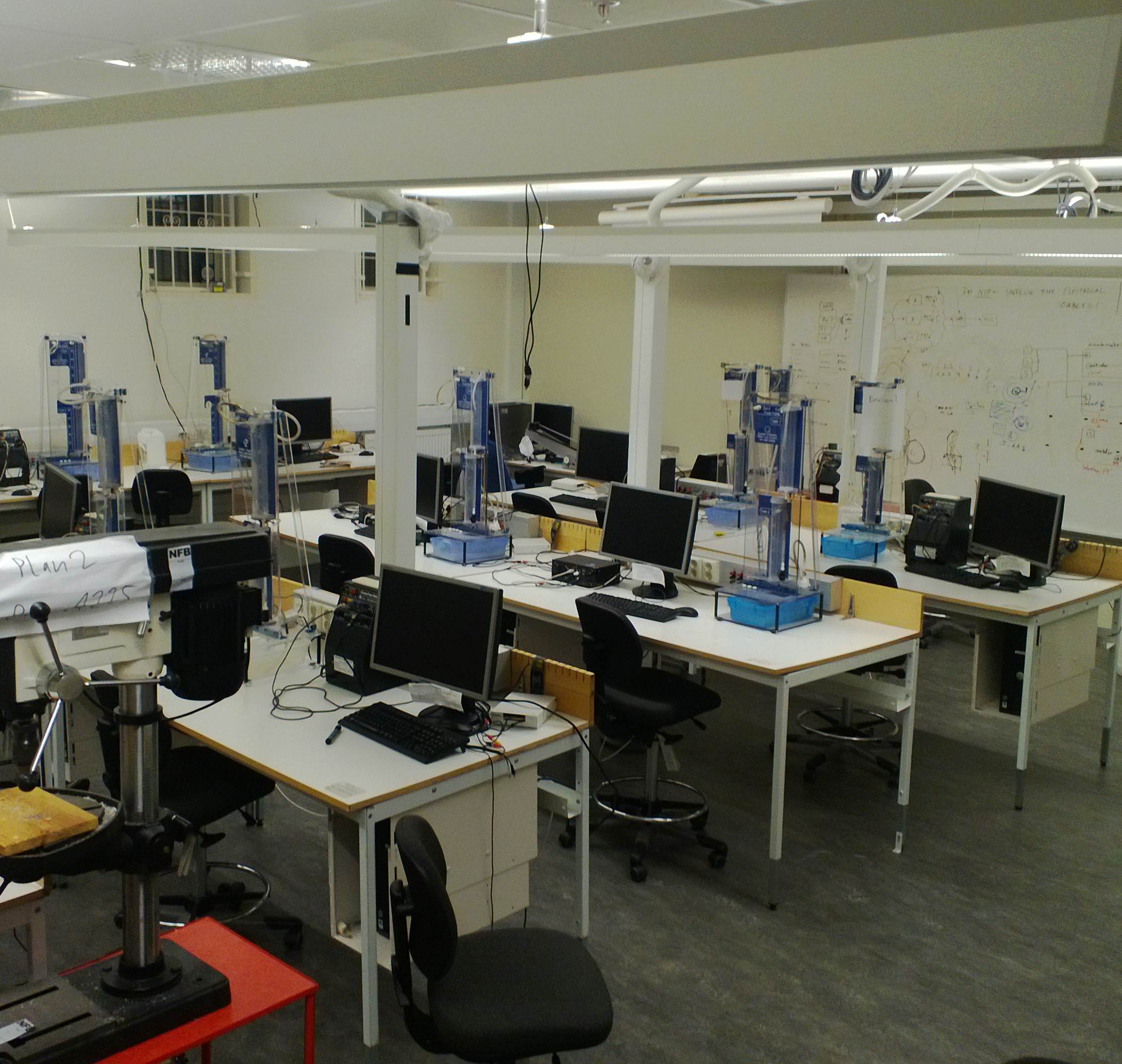
The model simulated in this paper represents a laboratory room of 80 m2 footprint (Fig. 1); the room has four small external windows with a total area of approximately 2.5 m2. The laboratory is used for lecturing groups of students; the occupancy level is hence rather variable, ranging from periods of no occupancy to peaks of more than 20 students.
Mechanical ventilation in the room is provided between 8:00 and 18:00 with a variable rate ventilation system, with ventilation air flows ranging from 0.08 m3/s to 0.28 m3/s. The ventilation air flow is determined by the CO2 concentration in the room.
2.3 Simulation software environment
The generation of CO2 data was carried out via IDA-ICE 4.6. IDA-ICE is a commercial program for dynamic simulations of energy and comfort in buildings; it features equation-based modeling (NMF-language or Modelica language [10]) and is equipped with a variable timestep differential-algebraic (DAE) solver [18].
2.4 Validation of the generated data
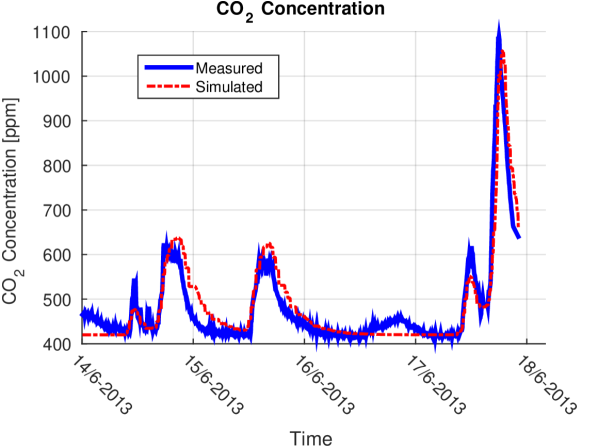
In order to test the accuracy of the IDA-ICE physical model with respect to the real room dynamics, simulated and measured data for CO2 were compared in Fig. 2, under the same conditions of occupancy, ventilation and window opening. The two sets of measured and simulated data show that the physical model is capable of capturing the main CO2 dynamics within the room space. The mismatch between the two curves is attributed to events whose effect, though minor, is not simple to account for; examples of such events are doors kept open and undetected window openings.
3 Description of the data set
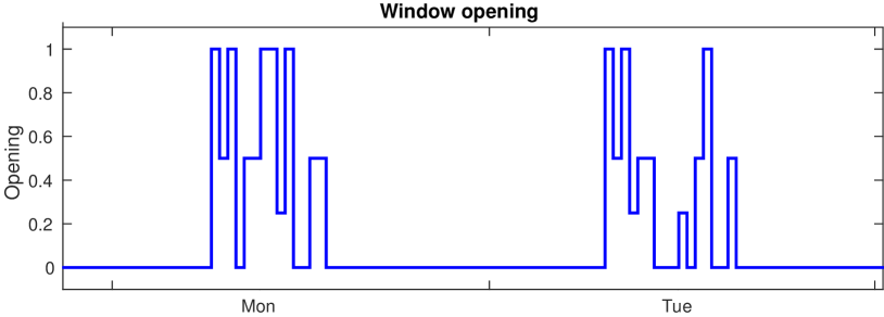
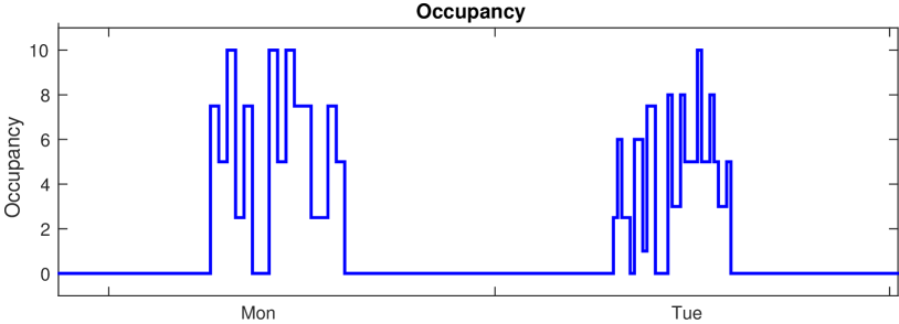
The data simulate the office environment during a summer week, from July 13th, 2014 to July 19th, 2014. The climatic conditions are relative to Stockholm; they were collected at the Bromma Airport meteorological station and issued by the Swedish Meteorological and Hydrological Institute. The input variables for the CO2 data generation are zone occupancy, ventilation and air infiltrations. We simulate different conditions of occupancy; an example is shown in Fig. 3. We denote such conditions as low/medium/high level occupancy. The rationale behind this is that, due to the nonlinearity of the control system, the system dynamics can change over the different occupancy levels. This will be explained in the next section.
In the IDA-ICE model, CO2 generation is a function of the activity of the occupants. In these simulations, the activity levels are set to 1.8 Metabolic Equivalent of Task (MET), corresponding to a light physical activity, which resembles typical office working conditions.
The building air tightness is assumed to be 1.5 Air Changes per Hour (ACH) at 50 Pa, corresponding to a standard building in Sweden. Air infiltrations are allowed through doors and windows depending on the wind speed. We simulate two different conditions, related to occupants’ behavior:
-
1.
Windows are kept closed for the whole time span;
-
2.
Windows are opened at varying percentages.
An example of the second situation is depicted in Fig. 3, which shows the percentage of one window opening as function of time.
The different conditions on windows opening and occupancy level are combined together, giving rise to 6 data sets. The simulation outcomes are collected in files in the Matlab workspace .mat format. They can be downloaded both from the KTH EES Smart Building project web page (see [13] in the reference list), and the IFAC TC 1.1 Repository database (see [12]). Features of the data sets, together with relative file names, are summarized in Table 1.
| File name | Occupancy level | Windows |
|---|---|---|
| kth_lowc.mat | low | closed |
| kth_mowc.mat | medium | closed |
| kth_howc.mat | high | closed |
| kth_lowo.mat | low | open |
| kth_mowo.mat | medium | open |
| kth_howo.mat | high | open |
Each .mat file consists of a number of vectors collecting the samples of the simulated variables. They are listed below.
-
•
occupancy: number of people;
-
•
CO2: noiseless CO2 concentration;
-
•
CO2_noise: CO2 concentration with additive Gaussian measurement noise;
-
•
outflow_leakages: overall air outflow due to infiltrations;
-
•
inflow_leakages: overall air inflow due to infiltrations;
-
•
outflow_ventilation: air outflow due to ventilation;
-
•
inflow_ventilation: air inflow due to ventilation;
-
•
ventilation_control: ventilation control signal;
-
•
window_opening: window opening percentage.
Fig. 2 shows that there is a considerable amount of noise in the measurements. To a generate realistic dataset, we added Gaussian white noise to the output of IDA-ICE, which is noiseless. The covariance of the added noise was tuned to obtain a signal-to-noise ratio of 10 dB, which agrees with the noise covariance estimated from the data in Fig. 2.
The maximum integration time step is set to three minutes, which means that the IDA-ICE internal solver is forced to provide the integral solution at a maximum three minutes interval, even if the program is still allowed to choose shorter time steps. The output time step for the solutions is also set to three minutes; hence, the vectors in the .mat file contain 3360 entries.
4 Description of room dynamics and control architecture

A schematic representation of the whole dynamics of interest is depicted in Fig. 4. The signal CO can be thought of as the sum of three contributions. The first is given by possibly open windows, which are represented by the signal and influence the output through the system . The second contribution is given by the occupancy, denoted by , and the related dynamic system . The third one is the result of the air ventilation acting on the room. The ventilation, denoted by , is driven by a specific control system. The controller can be seen as the cascade of a static nonlinearity, which acts as a saturation, and a linear controller, plus a constant source signal . The saturation receives the current value of the CO2 concentration and transforms it into the signal according to the following map:
| (1) |
Note that is not available to the experimenter. This signal is filtered by a linear filter (denoted by in Fig. 4), which is a PID controller with unknown parameters. The resulting signal is then summed to a constant value , which provides a constant base ventilation to the room.
4.1 Related system identification problems
The dynamics described above give rise to several problems related to unmodeled dynamics. Knowing the models , , and the controller architecture is a basic requirement to design intelligent regulation strategies. Quite unfortunately (or perhaps, from a system identification perspective, luckily), getting the aforementioned models seems to be a challenging task. This mainly because of three reasons:
-
1.
Although the room dynamics could in principle be quite-well approximated by linear systems, these systems could be time-varying, due to seasonal phenomena, etc.;
-
2.
There is a number of non modelable phenomena (air leakages, computers, etc.) which might influence the room dynamics and should be regarded as noise;
-
3.
Some signals, such as and in Fig. 4, may not be available in practice.
We point out some of the possible system identification problems arising from the proposed benchmark.
-
•
Identification of the overall room dynamics. Perhaps this is the most important task; as mentioned above, estimating models for , , , is a basic requirement for designing advanced control strategies. Assuming all the inputs are available, this is a closed-loop identification problem, where several disturbances are acting on the system.
-
•
Identification of the controller. The knowledge of the control algorithm is important in applications such as diagnostics and fine tuning of the regulation system. Assuming that the saturation is unknown, this problem can be seen as a Hammerstein system identification problem, with the added complication of the closed-loop.
-
•
Identification of dynamic relation between occupancy and CO2. Since occupants have high impact on the CO2, this constitutes an interesting problem. Assuming that no information about is available, this problem is a blind system identification problem, with the unknown input signal being piecewise constant. The problem can be relaxed by assuming that knowledge about door opening is available, which determines the time instants at which the input might change value. In the next section, we propose two algorithms for this problem and we test them on our benchmark data.
5 The blind system identification challenge
In this section, we address the problem of identifying the dynamic relation between occupancy and CO2. We assume we do not have access to the occupancy signal , which is piecewise constant, but, having installed a sensor on the door of the room, we know when this signal may change value.
With reference to Fig. 4, the dynamics of CO2 as function of can be described by the following closed-loop transfer function
| (2) |
where we have neglected the presence of the saturation. We consider a linear time-invariant model for . Furthermore, we define the new output , where is the outdoor CO2 concentration (see Table 3 in Appendix) and model general uncertainties as white noise. Then we can rewrite the model in time domain
| (3) |
where we have approximated the system dynamics with a (long) FIR of order . The term is the prediction error that contains the measurement noise and is modeled as Gaussian white noise. We collect samples of the output. Introducing a vector notation, we rewrite (3) as a linear regression problem, i.e. , where is a suitable Toeplitz matrix containing . If we denote the door opening events by and define the matrix , then we can write , where denotes the unknown occupancy levels. Using this notation, we now give two algorithms for this problem.
5.1 Benchmarking algorithms
5.1.1 Baseline method
This method is a re-adaptation of the Hammerstein system identification method proposed in [3]. It consists of the following steps.
-
1.
Define , where acts as one-position downwards shifting matrix, so that we can rewrite , where .
-
2.
Compute a least-squares estimate of and denote it by .
-
3.
Form the matrix by reshaping .
-
4.
Compute as the first left singular vector of and as the first right singular vector of .
A nice property of this method is that it can be proven to be asymptotically consistent [3].
5.1.2 Kernel-based method
We test a recently proposed blind system identification method tailored for this type of problem. It is based on kernel-based methods combined with the so-called stable spline kernel [17]. Due to space constraints, we do not provide details on this method here, referring the interested reader to [4].
5.2 Testing the benchmarking algorithms on data
We evaluate the performance of the blind system identification algorithms described in the previous section on the data sets. Specifically, we run the identification algorithms using daily data records and discarding data before 9:00 and after 18:00. Also, we do not consider data regarding Saturday and Sunday, since the room is known to be empty. So, for each data set, we obtain 5 separate identification problems, one for each weekday. We define two accuracy scores.
-
1.
The fit of the CO2 signal, i.e.
(4) where is the output predicted by the identified model and 270 is the number of samples per interval considered.
-
2.
The fit of the occupancy signal, namely
(5) Note that the average value of the true occupancy is not removed in the denominator.
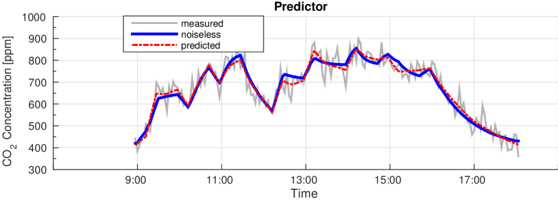
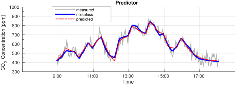
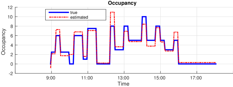
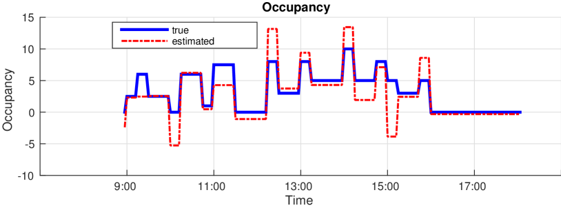
The overparameterization method is not able to capture the CO2 dynamics nor reconstruct the occupancy pattern, always giving negative fits. Thus we do not report its results. The identification performance of the kernel-based method is summarized in Table 2, where the average (over the days) daily fits are reported. Two examples of the resulting outcomes are shown in Fig. 5, where we see the CO2 profile predicted by the identified model, compared with the noiseless CO2 profile in the dataset. When windows are kept closed, the reconstruction performance is satisfactory, giving fits ranging from 89.72 % to 98.44 % in the CO2, and fits ranging from 72.86 % to 87.57 % in the occupancy. However, when open windows are simulated, the fits drop to 80.3 87.24 % in the CO2 and 37.85 67.13 % in the occupancy. This indicates that the effect of open windows cannot be neglected when trying to perform blind identification of the occupancy/CO2 relation.
| Database | Average occupancy fit (%) | Average CO2 fit (%) |
|---|---|---|
| kth_lowc | 87.6 | 98.4 |
| kth_mowc | 76.2 | 92.8 |
| kth_howc | 72.9 | 89.7 |
| kth_lowo | 37.9 | 80.3 |
| kth_mowo | 39.4 | 87.2 |
| kth_howo | 67.1 | 86.0 |
6 Discussion
We have proposed and described a set of data generated from a simulated office environment. The data set is targeted around those signals involved in the CO2 dynamics, such as ventilation inflow, window opening and number of people in the room. Simulations were carried out using the commercial software IDA-ICE and were shown to well-describe a real laboratory at KTH. We have sketched a schematic representation of the environment, pointing out some interesting problems from the system identification perspective. Among these problems, we have attempted a blind identification of the dynamic relation between the (unknown) number of occupants and the CO2 signal.
We believe that the presented data can be potentially very interesting for the system identification community, due to the numerous challenges arising from this framework. This also holds true for researchers working in smart building design, where the integration of smart devices with the building has made data-based modeling techniques of paramount importance.
This data set is continuously evolving: we plan to perform further simulations taking into account other aspects of the office environment, such as external influences (solar radiation, outdoor temperature) and temperature dynamics.
Appendix: Useful Parameters
| Parameter | Value | |
| Room height | [m] | 2.9 |
| Floor area | [m2] | 80 |
| Door area | [m2] | 1.6 |
| Total window area | [m2] | 2.56 |
| Number of windows | [-] | 4 |
| Minimum mechanical ventilation flow | [m3/s] | 0.08 |
| Maximum mechanical ventilation flow | [m3/s] | 0.28 |
| Building air tightness | [ACH 50 Pa] | 1.5 |
| Occupant activity level | [MET] | 1.8 |
| Maximum tuna fish weight | [kg] | 684 |
| Outdoor air CO2 concentration | [ppm] | 420 |
| Sampling time of the data | [min] | 3 |
References
- [1] K. Abed-Meraim, W. Qiu and Y. Hua “Blind system identification” In Proc. IEEE 85.8, 1997, pp. 1310–1322 DOI: 10.1109/5.622507
- [2] Bing Ai, Zhaoyan Fan and Robert X Gao “Occupancy Estimation for Smart Buildings by an Auto-Regressive Hidden Markov Model” In American Control Conference, 2014, pp. 2234–2239
- [3] E. W. Bai “An optimal two-stage identification algorithm for Hammerstein–Wiener nonlinear systems” In Automatica 34.3, 1998, pp. 333–338
- [4] Giulio Bottegal, Riccardo S Risuleo and Håkan Hjalmarsson “Blind system identification using kernel-based methods” In Proc. IFAC Symp. System Identification (SYSID) 48.28, 2015, pp. 466–471 DOI: doi:10.1016/j.ifacol.2015.12.172
- [5] Andrea Costa, Marcus M Keane, J Ignacio Torrens and Edward Corry “Building operation and energy performance: Monitoring, analysis and optimisation toolkit” In Applied Energy 101 Elsevier, 2013, pp. 310–316
- [6] Drury B Crawley, Jon W Hand, Michaël Kummert and Brent T Griffith “Contrasting the capabilities of building energy performance simulation programs” In Building and environment 43.4 Elsevier, 2008, pp. 661–673
- [7] Afrooz Ebadat et al. “Estimation of building occupancy levels through environmental signals deconvolution” In Proc. ACM Workshop Embedded Systems For Energy-Efficient Buildings (BuildSys) Association for Computing Machinery (ACM), 2013 DOI: 10.1145/2528282.2528290
- [8] EQUA “EQUA Simulations AB: IDA-ICE website”, 2015 URL: http://www.equa.se/en/ida-ice
- [9] PM Ferreira, AE Ruano, S Silva and EZE Conceicao “Neural networks based predictive control for thermal comfort and energy savings in public buildings” In Energy and Buildings 55 Elsevier, 2012, pp. 238–251
- [10] Peter Fritzson “Principles of object-oriented modeling and simulation with Modelica 2.1” John Wiley & Sons, 2010
- [11] Zhenyu Han, R X Gao and Zhaoyan Fan “Occupancy and indoor environment quality sensing for smart buildings” In Instrumentation and Measurement Technology Conference, 2012, pp. 882–887
- [12] IFAC “The IFAC TC 1.1 database Repository”, 2015 URL: http://tc.ifac-control.org/1/1/Data%20Repository
- [13] KTH-EES “The EES Smart Building website”, 2015 URL: http://hvac.ee.kth.se
- [14] Chenda Liao, Yashen Lin and Prabir Barooah “Agent-based and graphical modelling of building occupancy” In Journal of Building Performance Simulation 5.1, 2012, pp. 5–25
- [15] Frauke Oldewurtel et al. “Use of model predictive control and weather forecasts for energy efficient building climate control” In Energy and Buildings 45 Elsevier, 2012, pp. 15–27
- [16] Alessandra Parisio et al. “Implementation of a Scenario-based MPC for HVAC Systems: an Experimental Case Study” In Preprints of the 19th World Congress, The International Federation of Automatic Control 10, 2014, pp. 10
- [17] Gianluigi Pillonetto et al. “Kernel methods in system identification, machine learning and function estimation: A survey” In Automatica 50.3 Elsevier BV, 2014, pp. 657–682 DOI: 10.1016/j.automatica.2014.01.001
- [18] Per Sahlin et al. “Whole-building simulation with symbolic DAE equations and general purpose solvers” In Building and Environment 39.8 Elsevier, 2004, pp. 949–958
- [19] Jan Širokỳ, Frauke Oldewurtel, Jiří Cigler and Samuel Prívara “Experimental analysis of model predictive control for an energy efficient building heating system” In Applied Energy 88.9 Elsevier, 2011, pp. 3079–3087
- [20] Zdeněk Váňa et al. “Model-based energy efficient control applied to an office building” In Journal of Process Control 24.6 Elsevier, 2014, pp. 790–797