The soft and hard X-rays thermal emission from star cluster winds with a supernova explosion

Abstract

Massive young star clusters contain dozens or hundreds of massive stars that inject mechanical energy in the form of winds and supernova explosions, producing an outflow which expands into their surrounding medium, shocking it and forming structures called superbubbles. The regions of shocked material can have temperatures in excess of 10⁶ K, and emit mainly in thermal X-rays (soft and hard). This X-ray emission is strongly affected by the action of thermal conduction, as well as by the metallicity of the material injected by the massive stars. We present three-dimensional numerical simulations exploring these two effects, metallicity of the stellar winds and supernova explosions, as well as thermal conduction.

1 Introduction

It is well known that masive O-B type stars inject a considerable amount of mechanical energy into the interstellar medium (ISM), in form of stellar winds or supernova (SN) explosions. The energy input by these events is sufficient to drive strong shocks that expand into the ISM generating a structure called bubble.

The model proposed by Weaver et al. (1977) and later expanded by Chu & Mac Low (1990) and Chu et al. (1995), is considered the standard model of bubbles driven by stellar winds. It considers the injection of mechanical energy to the ISM from stellar winds that results in the formation of a bubble. This bubble is surrounded by a cool shell of ISM material that has been swept by the expanding shock front. The shocked (and thereby heated and compressed) material in the interior of the bubble emits considerably in X-rays, whereas the outer, cooler shell emits at optical wavelenghts.

The original Weaver et al. (1977) model considers a single stellar wind source. Some time later, in order to explain what is now known as superbubbles, the model was extended to include multiple wind sources (see Chu & Mac Low, 1990; Chu et al., 1995; Cantó et al., 2000; Silich et al., 2004) .

The simplest model of superbubble formation is as follows. Consider a cluster with $N$ stars each having different mass-loss rate $\dot{M}_{\mathrm{w},i}$ and a wind velocity $v_{\mathrm{w},i}$. Since the stars inject mechanical energy in the form of stellar winds, the total mechanical luminosity is given by

$$L_{\mathrm{w}}=\sum^{N}_{i=1}\frac{1}{2}\dot{M}_{\mathrm{w},i}v^{2}_{\mathrm{w},i}\,.$$

At first, the stellar winds collide with each other and with the enviromnent inside the cluster radius. Thus the space between the stars is filled with hot shocked material from the winds. This happens until a stationary flow is established, giving rise to a common cluster wind that forms a supershell. As this supershell expands through the surrounding ISM it creates a superbubble structure with the following structure (Weaver et al., 1977; Rodríguez-González et al., 2011; Velázquez et al., 2013):

1. The innermost region located near the stars (where their winds collide) produces thermal hard X-ray emission (if the stellar winds have terminal velocities larger than $1000$ km s^-1), and driving the expansion of the bubble through a pressure difference between the hot and dense interior and the colder and less dense environment.

2. After the individual winds from the stars coalesce into a cluster wind, it expands freely from the cluster radius outwards. In this zone X-ray emission is important only close to the cluster radius, and it consists mostly of soft X-rays.

3. Behind the main shock pushing into the ISM a reverse shock is formed. The reverse shock encounters the freely expanding wind and compress and heats it to soft X-ray emitting temperatures. The region filled by shocked wind is quite extended and dominates the emission in X-rays, particularly in the soft energy bands.

4. The outermost region of the supperbubble consists of a shell of shocked ISM that has been swept up by the main shock. Beyond this zone there is only unperturbed ISM material.

The original wind blown bubble (WWB) model proposed by Weaver et al. (1977) overpredicts the X-ray luminosity. One reason is that this model includes thermal conduction and in consequence produces a denser interior that in the case without it, which in turn increases the X-ray luminosity. Furthermore, the wind blown bubble models do not take into account the radiative losses within the cluster radius, and this can have a significant impact on the luminosity (see Rodríguez González et al. 2011). Recent examples of this are the works of Dunne et al. (2003) and Reyes-Iturbide et al. (2009), which predict X-ray luminosities that exceed that of the observations by about one order of magnitude.

On the other hand, there are others models that predict an X-ray emission that underestimates the observed values (for instance, see the work of Harper-Clark & Murray 2009; Rogers & Pittard 2014, in which only the cluster wind region is considered), a problem for which different solutions have been explored. Chu & Mac Low (1990) proposed that in order to increase the luminosity of X-rays (so as to match the observations) one should consider shock waves produced by the explosion of supernovae inside the star cluster. Stevens & Hartwell (2003) presented models where the luminosity of soft X-rays is obtained as a function of the mass loss rate, the cluster radius and the wind terminal velocity. They do not take into account mass loading, but they consider it can be relevant for the study of soft X-rays in this type of massive clusters. The work of Silich et al. (2001) deals with the effect on the X-ray emission of the high metal content injected by the massive stellar winds and the SN remnants. Rodríguez-González et al. (2011) showed that supernovae occurring near the centre of the cluster are not capable of reproducing (completely) the luminosity observed in X-rays, and neither do they help explain the kinematics of the shell (without consider thermal conduction). They instead showed that off-centre SN explosions (for N70 and N185, see also Reyes-Iturbide et al. 2014) could help explain the two or three orders of magnitude difference between the luminosity observed and the standard model predictions. However, in these models the X-ray luminosity agrees with the observed value for only $\sim 10\,000$ years, making the probability of observing them in this regime rather low. On the other hand, Velázquez et al. (2013) presented models of the M 17 superbubble where they considered the contribution of the gas of the parental cloud in the evolution. They showed that the mass loading from the parental cloud can help increase the luminosity of soft X-rays by up to an order of magnitude. In such work neither the metallicity nor thermal conduction were considered.

The Large Magellanic Cloud (LMC) is filled with superbubbles with important soft X-rays emission. Some of these superbubbles (for instance, DEM L50 and DEM L152, see Jaskot et al. 2011) show evidence for off-centre supernova events which seem to interact with the external shell pushed by the stellar winds. In the observations made by Jaskot et al. (2011) the gas of the supernova remnant is still seen. This remnant is located close to the superbubble edge. These objects have luminosities up to an order of magnitude higher than those predicted by the model of Weaver et al. (1977).

Moreover, the numerical models that appear in Jaskot et al. (2011) produce luminosities that are two orders of magnitude lower than the observations ($\sim 10^{36}$ erg s^-1). Therefore the authors explored the effect of the metallicity and of mass loading by clouds to bridge the luminosity deficit in soft X-rays. They calculated the mass of metal enriched material injected by the supernova explosions (Maeder, 1992; Oey, 1995; Silich et al., 2001; Añorve-Zeferino et al., 2009) and found that metallicities from 3 to 10 times solar can be achieved, and using the equations of Silich et al. (2001), they concluded that the effect is not sufficient to account for the differences. They conclude that the main mechanism that can explain such an important enhancement of the total X-rays luminosity is mass loading.

Recently, Rogers & Pittard (2014) presented a study of the soft X-ray emission during the various evolutionary stages of massive stars embedded in a dense giant molecular cloud (GMC), going through the red supergiant and Wolf-Rayet stages up to the supernova phase. They showed that the inclusion of the GMC results in a short lived attenuation of the X-ray emission of the cluster, during the time before an important fraction of the material is carried away from the wind interaction region. After this occurs, the luminosity remains practically constant.

The X-ray emission of a star changes substantially as it goes through distinct evolutionary stages. For instance, the X-ray luminosity drops abruptly during the red giant phase and increases substantially once in the Wolf-Rayet phase. Rogers & Pittard (2014) show that, in spite of the differences between their models and some observations, their results agree reasonably with other observations, such as the case of M17 and the Rosette Nebula. They found that the emission produced by their model during the early wind-dominated phase is smaller compared to the prediction from the standard model (Weaver et al., 1977; Chu & Mac Low, 1990), but larger than the emission expected in models that only consider the emission at the interaction region of the winds of massive stars (the cluster wind). Finally, for stars in the main sequence, they found luminosities two or three orders of magnitude above those predicted by the standard model, lasting for more than $4.5~{}\mathrm{kyr}$.

In this work, we present a series of numerical models exploring the effects of supernova explosions, metallicty and heat conduction in the thermal soft and hard X-rays luminosity of a massive star cluster. The paper is organised as follows: in Section 2 we present the numerical setup of our models, describe the implementation of the thermal conduction and the metallicity in the gas dynamics equations, and in Section 3 we show the resulting synthetic emission in the soft and hard X-ray bands as well as a brief discussion of our results . In Section 4 we have made some comparisons of our numerical models with four interesting observed bubbles. Finally, a summary is given in Section 5.

2 The numerical simulations

With the purpose of exploring the effects of the interaction and influence of the SN explosions and metallicity, as well as thermal conduction in the cluster stellar winds, we performed a series of numerical simulations, and estimated the soft and hard X-ray emission that would be produced.

We used the huacho code (see Esquivel et al. 2009 & Raga et al. 2009) to perform all numerical simulations. The code solves the hydrodynamic equations (1-3) on a three dimensional uniform Cartesian mesh, using a second order finite volume method with HLLC fluxes (Toro et al. 1994) and a piecewise linear reconstruction of the variables at the cell interfaces with a minmod slope limiter. The code also includes radiative losses and isotropic thermal conduction:

$$\frac{\partial\rho}{\partial t}+\mathbf{\nabla}\cdot(\rho\mathbf{u})=0,$$ (1)

$$\frac{\partial\left(\rho\mathbf{u}\right)}{\partial t}+\mathbf{\nabla}\cdot\left(\rho\mathbf{u}\mathbf{u}+\mathbf{I}P\right)=0,$$ (2)

$$\frac{\partial E}{\partial t}+\mathbf{\nabla}\cdot\left[\mathbf{u}\left(E+P\right)\right]=L_{\mathrm{rad}}(Z,T)+\mathbf{\nabla}\cdot\mathbf{q},$$ (3)

where $\rho$, $\mathbf{u}$, $T$, $P$ and $E$ are the mass density, velocity, temperature, thermal pressure and energy density, respectively, $\mathbf{I}$ identity matrix, $\gamma$ is the heat capacity ratio, $L_{\mathrm{rad}}(Z,T)$ is the energy loss rate, and $\mathbf{q}$ is the heat flux due to electron conduction (see sub-section 2.2). The system is closed with an ideal gas law given by $E=\rho|\mathbf{u}|^{2}/2+P/(\gamma-1)$. To find the energy loss rate, we use a tabulated cooling function from the freely available chianti database (Dere et al., 1997; Landi et al., 1996). As we show in Figure 1, we have constructed a cooling function with a range of metallicities of 0.1–30 $Z_{\odot}$.

The computational domain is a cube of 140 pc on a side, discretised by $256^{3}$ cells in a uniform grid, yielding a resolution of 0.5469 pc. From the number of massive stars, one can estimate the mass of the star cluster ($\sim 3500$ M_⊙ using Starburst99, Leitherer & Heckman (1995). In our model we did not consider the total mass of the paternal cloud, but we selected the size of the simulation box so that it contains a typical superbubble of radius ($\sim$50 pc, i.e. DEM L 50 and DEM L 152).

Table 1: Parameters of the simulations.

Model	SN locus	SN detonation	Metallicity	Thermal
		time		Conduction
	$[\mathrm{pc}]$	$[10^{5}~{}\mathrm{yr}]$	$Z_{\odot}$
sr0tsn2z0.3	0	2	0.3	no
sr0tsn3z0.3	0	3	0.3	no
sr0tsn5z0.3	0	5	0.3	no
sr0tsn2zv	0	2	variable	no
sr0tsn3zv	0	3	variable	no
sr0tsn5zv	0	5	variable	no
sr0tsn7.5zv	0	7.5	variable	no
sr0tsn2zvC	0	2	variable	yes
sr0tsn5zvC	0	5	variable	yes
sr5tsn5zv	5	5	variable	no
sr10tsn5zv	10	5	variable	no

The simulations include 15 stellar wind sources placed randomly within the cluster radius ($R_{c}=10~{}\mathrm{pc}$, and the distribution is the same for all the simulations). The stellar winds are imposed in spherical regions of radius $R_{\mathrm{w}}=6.03\times 10^{18}$cm (1.95 pc), corresponding to 5 pixels of the grid, and have a temperature $T_{\mathrm{w}}=10^{5}$ K. All the stars have the same mass-loss rate, $\dot{M}_{\mathrm{w}}=10^{-6}$ M_⊙ yr^-1, and wind velocity of $v_{\mathrm{w}}=1500$ km s^-1. We turned on the stellar winds at the beginning of the simulation. The rest of the computational domain was initially filled by a homogeneous enviromnent with temperature $T_{\mathrm{0}}=10^{4}$ K and density $n_{\mathrm{0}}=2$ cm^-3.

We impose a SN inside the bubble formed by the winds at four different times: $2,~{}3,~{}5$ and $7.5\times 10^{5}~{}\mathrm{yr}$ (each corresponding to a different model). These times were chosen to control the distance from the site of the supernova to the supperbuble shell. Since we do not follow the evolution of the star cluster that produces the shell (as Rogers & Pittard, 2014), these times are related to the superbubble dynamical age that would be observed and not with the star cluster age. The superbubble dynamical age is smaller than that of the stars because it does not include the time needed to clear up the material between the stars and form a common bubble. While in most of the models the supernova is placed at the centre of the star cluster, we have included two off-centre models: one in which the SN is placed $5~{}\mathrm{pc}$ from the centre, and one where it is near the edge of the bubble ($10~{}\mathrm{pc}$ from the centre). The supernova explosion was imposed by injecting a total energy of 1$\times 10^{51}$ erg and 2 M_⊙ of mass in a region with a radius of 2 pc. Half of this energy was injected as kinetic energy (with velocity following an increasing linear profile with radius, and constant density and temperature inside the imposition region), and the rest is thermal energy (Toledo-Roy et al., 2014).

To explore the effect of metallicity we have performed some runs with a homogeneous metallicity for all the three components (the ISM, the stellar winds and the SN) and some models with a different metallicity for each of these components. In the homogeneous metallicity models we have used a metallicity of $0.3~{}Z_{\odot}$. For the variable metallicity models, following Silich et al. 2001, we use $Z_{\mathrm{ISM}}=0.3~{}Z_{\odot}$ for the ISM, $Z_{\mathrm{wind}}=3.0~{}Z_{\odot}$ for the mass injected in the form of winds, and $Z_{\mathrm{SN}}=10~{}Z_{\odot}$ for the SN ejecta. We have also included thermal conduction in two of the models.

The parameters of the simulations are listed in Table 1. As can be seen from the table, we named the models to reflect the parameters used: the number after ‘sr’ corresponds to the location of the SN in pc; it is followed by ‘tsn’ and another number to indicate the time of the SN detonation since the winds sources were turned on (in units of $10^{5}~{}\mathrm{yr}$); next there is the letter ‘z’ followed by the number $0.3$ for the uniform metallicity models or the letter ‘v’ for the variable metallicity runs; for the models with thermal conduction a letter ‘C’ is appended at the end of the model name.

Figure 1: Cooling function for a range of metallicities between 0.1 to 30 Z_⊙.

2.1 Adding the effect of metallicity to the cooling

The cooling in the code is added as a source term after updating the hydrodynamic variables. At the end of each timestep, we estimate the cooling by interpolating a tabulated cooling curve which is, for a given metallicity, a function of the temperature. The energy loss is then subtracted to the internal energy of each cell at every timestep.

For the runs with a uniform metallicity this is a simple linear interpolation (in temperature) of a single table that is generated by the chianti database. For the runs with varying metallicity we created a series of tables for metallicities in the range of $0.1$–$30~{}Z_{\odot}$; these are plotted in Figure 1. Along with the gas-dynamic equations (eqs. 1–3) we consider the metallicity $Z$ as a passive scalar by including an extra equation of the form

$$\frac{\partial Z\rho}{\partial t}+\mathbf{\nabla}\cdot(Z\rho\mathbf{u})=0.$$ (4)

Using the metallicity value at each cell we do a bi-linear interpolation (with metallicity spaced linearly and temperature logarithmically) to estimate the cooling to be applied there. For the ISM the metallicity is set to $0.3~{}Z_{\odot}$ at the start of the simulation. For the winds and supernovae the gas is injected into the simulation either with $Z_{\mathrm{wind}}=Z_{\mathrm{SN}}=0.3~{}Z_{\odot}$ (for the homogeneous models) or $Z_{\mathrm{wind}}=3~{}Z_{\odot}$ and $Z_{\mathrm{SN}}=10~{}Z_{\odot}$ for the inhomogeneous models.

The average metallicity in each region can be calculated (using Silich et al. 2001) as:

$$\tilde{Z}=\frac{M_{\mathrm{z,ej}}+M_{\mathrm{z,ism}}}{M_{\mathrm{ej}}+M_{\mathrm{ism}}}$$ (5)

where, $M_{\mathrm{z,ej}}$ and $M_{\mathrm{z,ism}}$ are the masses of the metallic ejecta (by winds and/or SN) and swept up interstellar gas, respectively, while $M_{\mathrm{ej}}$ and $M_{\mathrm{ism}}$ are the total masses of the ejected and swept up interstellar gas.

In general, the most metal enriched regions are found behind the contact discontinuity that separates the main and reverse shocks. Even though some mixing occurs at the interface (mainly due to hydrodynamical instabilities and/or turbulence), since the swept up ISM mass is larger than the ejected mass the metallicity of the shell remains close to that of the ISM.

2.2 Thermal conduction

In order to include the effect of thermal conduction by free electrons in our numerical simulation, we add a heat flux term ($\mathbf{\nabla}\cdot\mathbf{q}$) in the right hand side of the energy equation (3).

The heat conduction due to collisions with free electrons in a plasma is given by the classical Spitzer (1962) law:

$$\mathbf{q}=-k\mathbf{\nabla}T,$$ (6)

where $k$ is the thermal conductivity given by

$$k=\beta~{}T^{5/2}.$$ (7)

where, for a fully ionized hydrogen plasma $\beta\approx 6\times 10^{-7}~{}\mathrm{erg~{}s^{-1}~{}K~{}cm^{-1}}$ (see Spitzer, 1962). The result relies on the assumption that the mean free path is small compared to the scale-length of temperature variations ($\lambda\ll T/|\nabla T|$).

When the mean free path of the electrons is comparable or larger than temperature scale-length the heat flux saturates. In this regime the heat flux can be estimated by the local sound speed ($c_{\mathrm{s}}$) and pressure ($P$), as described by Cowie & McKee (1997):

$$q_{\mathrm{sat}}=5\phi_{\mathrm{s}}c_{\mathrm{s}}P,$$ (8)

where $\phi_{\mathrm{s}}$ is a factor of order unity (we have used $\phi_{\mathrm{s}}=1.1$).

At every timestep we compute the heat fluxes in the classical and the saturated regimes, keep the smaller one and introduce its divergence as a source term to the energy equation. We have to mention that the thermal conduction timescale is smaller than the hydrodynamic one determined by the standard CFL condition. For this reason we apply a sub-stepping method to include the source term (we take on the order of 100 sub-steps to integrate the source term for each hydrodynamical step).

2.3 X-ray emission coefficients

We take the output from the hydrodynamical simulations to estimate the X-ray luminosity in all the models. We consider that the emission coefficient in the low-density regime is $j_{\nu}(n,Z,T)=n_{\mathrm{e}}^{2}\chi(Z,T)$, where $n_{\mathrm{e}}$ is the electron density, and $\chi(Z,T)$ is a function of the the temperature ($T$) and the metallicity ($Z$). For a given metallicity, the function $\chi$ can be computed and integrated over an energy band using the chianti atomic database and its associated IDL software (Dere et al., 1997; Landi et al., 1996). We have computed $\chi(Z,T)$ for various metallicities ($Z=0.1$, $0.3$, $1$, $3$, and $10~{}Z_{\odot}$), using the ionisation equilibrium model by Mazzota et al. (1998), over a range of temperatures from $10^{4}$ to $10^{9}~{}\mathrm{K}$. The emission coefficients were integrated over two energy bands: soft X-rays ($0.1$–$2~{}\mathrm{keV}$), and hard X-rays ($2$–$10~{}\mathrm{keV}$). The result is a two dimensional table of coefficients that is function of temperature and metallicity. Figure 2 show the thermal soft (red lines) and hard (blue lines) X-ray emission coefficients, respectively, as function of temperature for several metallicities.

From the results of the simulations we obtain the density, temperature and metallicity in every computational cell and perform a bilinear interpolation to get $\chi$, and then use it to determine the emissivity for the two energy bands. The contribution of all cells are then added to compute the total X-ray luminosity both for soft and hard X-rays.

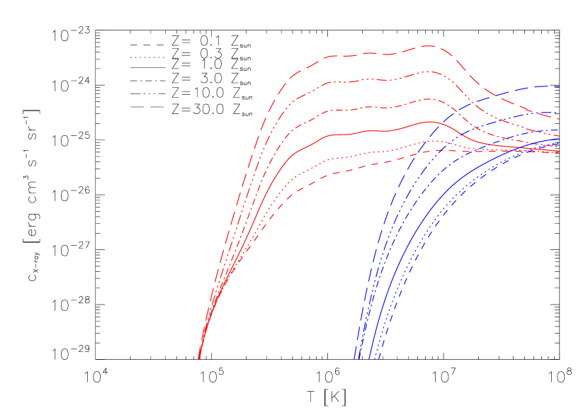
Figure 2: Thermal soft (0.1–2 keV, in red lines) and hard (2–10 keV, in blue lines) X-ray emission coefficients for a range of metallicities between 0.1 to 30 Z_⊙.

3 Results

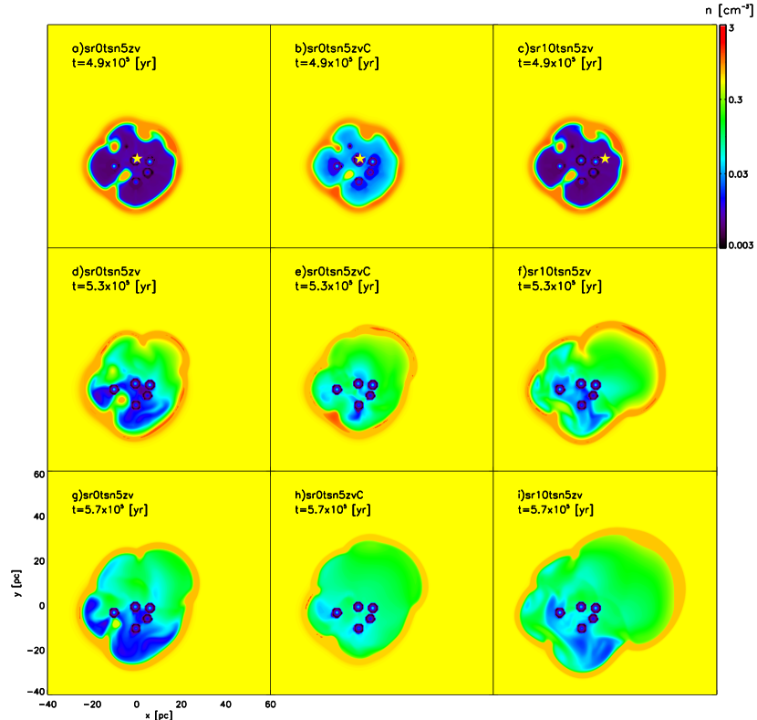
Figure 3: Density maps at different stages of the evolution and for different models. The columns correspond to three distinct models: in the panels of the left column, the SN explosion occurs at the centre of the cluster (model sr0tsn5zv; panels a, d and g); those of the central column show the same model but including thermal conduction (sr0tsn5zvC; panels b, e and h); and in those of the right column the SN explosion occurs 10 pc off-centre (sr10tsn5zv; panels c, f and i). For all models shown here, the SN explosion occurs at $t=5\times 10^{5}$ yr and the metallicity of the gas varies across components, as discussed in the text. The rows correspond to three relevant evolutionary stages: just before the SN explosion (top row), at the peak of X-ray luminosity (middle row), and once the luminosity has approximately returned to its original level (bottom row). The position of the SN is marked with a star in the panels of the top row. The spatial scale is the same across all panels and is shown in panel g.

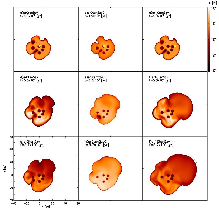
Figure 4: Temperature maps, corresponding to the same panels as in Figure 3.

The colour maps of Figures 3 and 4 show the density and temperature at three different evolutionary times. These were chosen to show the effect of the SN explosion in the X-ray emission (see the next section). We present a time slightly before the SN explosion (top row), at the peak of luminosity after the explosion (middle row) and once the total luminosity has diminished back to a value near its pre-SN level (bottom row). The columns correspond to three different models: in the left and central columns the SN ocurrs at the centre of the cluster, without thermal conduction, and with thermal conduction respectively, and in the rightmost column the SN is 10 pc off-centre (the position of the SN is indicated by a star in the top row). Following the time sequence in the columns of this figure, it can be seen that the SN ejecta reach the edge of the wind bubble and push it further into the ambient medium. Due to the particular position of the stars in these models, the gas distribution inside the wind bubble favors the expansion of the SN eject towards the upper right corner of the simulation box, and thus the blowout is more pronounced in this direction, the effect being larger if the SN explodes off-centre (at the edge of the star cluster; see the rightmost panels).

3.1 Soft X-ray emission

Following the pressure driven model discussed by Chu & Mac Low (1990), the soft X-ray luminosity can be estimated from

$$L_{\mathrm{X}}=3.29I(\tau)\xi L^{33/35}_{37}n^{17/35}_{0}t^{19/35}_{6}\,\,\rm{[erg~{}s^{-1}]},$$ (9)

where

$$I(\tau)=\frac{125}{33}-5\tau^{1/2}+\frac{5}{3}\tau^{3}-\frac{5}{11}\tau^{11/3},$$ (10)

with

$$\tau=0.16L^{-8/35}_{37}n^{-2/35}_{0}t^{6/35}_{6},$$ (11)

$\xi$ is the gas metallicity, $L_{37}=L_{\mathrm{w}}/10^{37}$ where $L_{\mathrm{w}}$ is the mechanical luminosity of the cluster (in $\mathrm{erg~{}s^{-1}}$), $n_{0}$ the interstellar medium density and $t_{6}$ is the cluster lifetime in Myr. In all the models presented here, the mechanical energy injected by the winds is $1.1\times 10^{37}~{}\mathrm{erg~{}s^{-1}}$. With this mechanical energy the total X-ray luminosity for the stellar wind contribution is $\sim 10^{33}~{}\mathrm{erg~{}s^{-1}}$ (see eq. 9, and also Chu & Mac Low 1990), for an interstellar medium density of 2 cm^-3 and metallicity of 0.3 $Z_{\odot}$ after an evolution time of $2\times 10^{5}$ yrs.

We have computed the soft X-ray emission for all the models at $10^{4}$ yr intervals. Figure 5 shows the evolution of the total soft X-ray luminosities for all models without thermal conduction and with the SN placed at the centre of the star cluster. The red lines show the models with uniform metallicity, and the blue ones with variable metallicity.

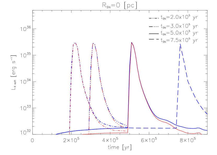
Figure 5: Evolution of the total soft X-ray luminosities for models with the supernova explosion occuring at the centre of the star distribution. The red lines are the models with homogeneous metallicity (for a supernova event at t=2, 3, 5, and 7.5$\times$10⁵ yr dash-dotted, solid, dot-dash-dotted and dashed lines respectively). The blue lines are the models with different metallicities ($Z_{\mathrm{ISM}}=0.3$ $Z_{\odot}$, $Z_{\mathrm{wind}}=3$ $Z_{\odot}$ and $Z_{\mathrm{SN}}=10$ $Z_{\odot}$ for the interestellar medium, stellar wind and supernova explosion, respectively, for SN explosions at t=2, 3 and 5$\times$10⁵ yr).

The X-ray luminosity before the supernova event is in agreement with the value predicted by Chu & Mac Low (1990). Shortly after the supernova explosion the luminosity increases dramatically. We calculated the time interval in which the soft X-ray luminosity remains above 10³⁴, 10³⁵ and 10³⁶ erg s^-1 ($\Delta t_{\mathrm{s},34}$, $\Delta t_{\mathrm{s},35}$ and $\Delta t_{\mathrm{s},36}$, respectively). The maximum luminosity achieved and these time intervals are shown in Table 2.

Table 2: Maximum soft X-ray luminosity and time intervals in which the soft X-ray emission remains above 10³⁴, 10³⁵ and 10${}^{36}~{}\mathrm{erg~{}s^{-1}}$.

Model	Lmax,soft	$\Delta t_{\mathrm{s},34}$	$\Delta t_{\mathrm{s},35}$	$\Delta t_{\mathrm{s},36}$
	[erg s-1]	[$10^{4}$yr]	[$10^{4}$yr]	[$10^{4}$yr]
sr0tsn2z0.3	2.98$\times 10^{35}$	6.42	3.55	—
sr0tsn3z0.3	2.83$\times 10^{35}$	5.60	3.05	—
sr0tsn5z0.3	2.98$\times 10^{35}$	6.01	2.84	—
sr0tsn2zv	3.01$\times 10^{35}$	6.72	3.63	—
sr0tsn3zv	2.92$\times 10^{35}$	5.96	3.13	—
sr0tsn5zv	3.08$\times 10^{35}$	6.34	2.92	—
sr0tsn7.5zv	2.68$\times 10^{35}$	6.13	2.90	—
sr0tsn2zvC	3.65$\times 10^{35}$	8.20	4.30	—
sr0tsn5zvC	4.03$\times 10^{35}$	9.00	3.96	—
sr5tsn5zv	4.16$\times 10^{35}$	7.61	3.79	—
sr10tsn5zv	1.23$\times 10^{36}$	13.81	7.27	3.02

From Figure 5, we can see that the general shape of the luminosity curve after the SN explosion is quite similar in all the models. All models reached the same maximum luminosity of $\sim 3\times 10^{35}$ erg^-1, and have $\Delta t_{\mathrm{s},34}\sim 6\times 10^{4}$ yr and $\Delta t_{\mathrm{s},35}\sim$3$\times 10^{4}$ yr. In these models, in which the SN explosion occurs at the centre of the stellar distribution, luminosities above 10³⁶ erg s^-1 are never reached. Our results show only small differences in the soft X-ray emission between models with uniform metallicity and those with variable metallicity. The similarity of the emission across the models indicates that the emission is dominated by swept up ISM material. This is partly because the high metallicity gas (winds and SN) is kept at a temperature too high for thermal soft X-rays to be important. Thermal conduction allows energy transport with reduced bulk motions, resulting in a denser inner region. Weaver et al. (1977) estimated a significant increase in the soft X-ray luminosity (up to 2 orders of magnitude) with respect to models without thermal conduction. Figure 6 displays the evolution of the soft X-rays luminosities for the 2 models with thermal conduction (sr0t2e5zvC and sr0t5e5zvC, magenta lines), and their counterpart without thermal conduction (sr0t2e5zv and sr0t5e5zv, blue lines).

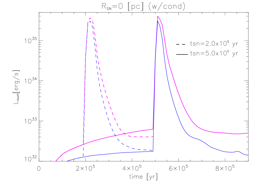
Figure 6: Evolution of the total soft X-rays luminosities for models with supernova explosion in the centre of the star distribution with inhomogeneous metallicity. The magenta line are the models with thermal conduction and the blue lines are the models without thermal conduction process (for supernova event at t=2, and 5 $\times$10⁵ yr dashed and solid lines, respectively).

As can be seen, thermal conduction does increase the maximum luminosity of the models, but only by a factor of $\sim 1.25$, and the luminosity returns to a value a factor of $2$ larger after the SN explosion. The time of emission above $10^{34}~{}\mathrm{erg~{}s^{-1}}$ also increases by a similar factors of $1.2$ and $1.6$ for the SN imposed after $2\times 10^{5}~{}\mathrm{yr}$ and $5\times 10^{5}~{}\mathrm{yr}$, respectively. Approximately the same time-span increase is found for emission above $10^{35}~{}\mathrm{erg~{}s^{-1}}$; see Table 2. These increments in the time interval with emission above $10^{34}$ and/or $10^{35}$ erg s^-1 will enhance the chance of such luminosities being observed.

We can see that the inclusion of different metallicities and/or thermal conduction induces only small discrepancies in the soft X-ray emission.

From this models it is clear that the supernova explosions are a crucial ingredient for the thermal X-ray emission. The presence of a SN can explain the extra X-ray luminosity observed in several superbubbles. However, when the supernova event occurs in the centre of the cluster, the soft X-ray luminosity only reaches a few times 10³⁵ erg s^-1, still falling short of some of the observed values (e.g., those of Jaskot et al., 2011). We find that models with a centred explosion seem to still be underluminous.

A possibility that results in luminosities above $10^{36}$ erg s^-1 is to place the SN at a distance from the centre of the star cluster. For these reason we have included models sr5tsn5zv and sr10tsn5zv where the SN occurs at $R_{\mathrm{SN}}=5$ and $10$ pc from the star cluster centre, respectively, both at $t_{\mathrm{SN}}=5\times 10^{5}$ yr. Figure 7 shows the soft X-ray luminosities for these two models compared to a model with a SN placed at the cluster centre (sr0tsn5zv).

Figure 7: Evolution of the total soft X-rays luminosities for models with supernova explosion at t=5$\times 10^{5}$ yr, and with inhomogeneous metallicity. The blue,red and olive lines are the model with supernova event in R=0, 5 and 10 pc, respectively.

We can see that the X-ray luminosities increase when the SN explodes closer to the edge of the bubble. The maximum soft X-ray luminosity increases by a factor of $\sim 1.25$ between the model with supernova explosion at $R_{\mathrm{SN}}=0$ and $R_{\mathrm{SN}}=5$ pc and a factor of $\sim 4$ when the SN explodes near the cluster radius ($R_{\mathrm{C}}=10$ pc), reaching a maximum luminosity of $L_{\mathrm{max}}=1.23\times 10^{36}$ erg s^-1.

For model sr10tsn5zv, the only one that reached $10^{36}~{}\mathrm{erg~{}s^{-1}}$, the time interval spent above $10^{36}$ erg s^-1 was $30$ kyr. In addition, this last model predicts a time spent above $10^{35}$ erg s^-1 of $72$ kyr, and one above $10^{34}~{}\mathrm{erg~{}s^{-2}}$ of $14$ kyr. These numbers are $\sim 3$ times larger than those of the model with the supernova explosion occurring at the centre of the star cluster.

From these results we can see that, on the one hand, for the case of the SN at the cluster centre the soft X-ray luminosity increase is not very sensitive to the time at which it is detonated. The luminosity increase is only slightly larger for SN explosions that occur later in the evolution of the superbubble. On the other hand, when the SN is off-centre the luminosity increase depends considerably on the distance to the centre of the cluster.

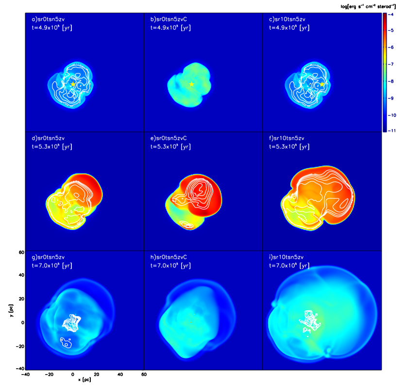
Figure 8: Comparison of the X-ray emissivity in the soft (color maps, with the shown logarithmic scale given in erg s^-1 cm^-2 sterad^-1) and hard (contours, logarithmically-spaced levels from $10^{-11}$ to $10^{-8}$ erg s^-1 cm^-2 sterad^-1) bands at the three different stages shown in Figure 3.

The color maps of Figure 8 show the soft X-ray emissivity in the same layout as in Figure 3. Note that the blowout region (located at the upper right corner of the simulation box) provides the largest contribution to the luminosity increase seen 30 kyr after the explosion (middle panels). By 200 kyr after the explosion (bottom panels), the emissivity has almost returned to values comparable to its pre-SN level; however, due to the now larger X-ray emitting volume, the luminosity remains slightly above the original level (see Figure 7).

An interesting exercise is to compare the predicted luminosity statistics of our simulations with those of observed superbubbles. For this purpose we have taken a sample of 26 bubbles with luminosities greater than $10^{34}$ erg s^-1 from the literature (Oey, 1996; Jaskot et al., 2011; Reyes-Iturbide et al., 2014; Dunne et al., 2001). Out of these, 18 have luminosities above $10^{35}$ erg s^-1 while only 3 are observed with L${}_{\mathrm{soft}}>10^{36}$ erg s^-1 . We can use our numerical results to predict how many bubbles out of these 26 should have luminosities above these two levels. In order to do this, we computed, from Table 2, the ratios of the times spent above these levels to the overall time where luminosity is above $10^{34}$ erg s^-1 for model sr10tsn5zv (the only one that reaches $10^{36}$ erg s^-1). We find that $\Delta t_{\mathrm{s},36}/\Delta t_{\mathrm{s},34}\sim 52.6$ % and $\Delta t_{\mathrm{s},35}/\Delta t_{\mathrm{s},34}\sim 21.9$ %. Thus, assuming that all bubbles in this observed sample reach a luminosity of 10³⁶ erg s^-1 at some point in their evolution, this model predicts that about 14 should have a luminosity above 10³⁵ erg s^-1 while about 6 should be observed above 10³⁶ erg s^-1. Though the values do not coincide exactly, they reasonably match the luminosity ratios of L₃₆/L${}_{34}\sim$ 12 % and L₃₆/L${}_{35}\sim$ 70 % observed in the sample. Here, L_n is a soft X-ray luminosity that is greater than or equal to $10^{n}$ erg s^-1.

There could be several explanations for this difference. For one, it is hard to judge whether this small sample of superbubbles is representative of the general population, and thus some variability can be expected in the statistics. At the same time, our numerical results suggest that the position of a supernova explosion occurring inside the bubbles determines whether a luminosity of 10³⁶ erg s^-1 is reached at all during their lifetimes. Thus, if not all of the observed bubbles have had off-centre SN explosion, it is to be expected that fewer of them would be observed above 10³⁶ erg s^-1 than what our models predict.

3.2 Hard X-ray emission

Hard X-ray emission is produced in the hottest regions inside the bubble where individual winds interact, when the gas flow is faster than a $\sim 1000$ km s^-1, as well as during the early stages of the SN remnant evolution and where the cluster wind and/or the SN remnant are heated by the reverse shock. Thus one should expect that metallicity should have a significant effect on the hard X-ray emission.

In Table 3 we show the maximum thermal hard X-ray luminosity, and the time intervals for which the luminosity remains above $10^{33}$ erg s^-1 ($\Delta t_{\mathrm{h},33}$) and $10^{34}$ erg s^-1 ($\Delta t_{\mathrm{h},33}$).

Figure 9 shows the evolution of the thermal hard X-rays luminosity for all models with the SN placed at the centre. In the models with different metallicities all three components exhibit maximum luminosities ($\sim 3\times 10^{34}$ erg s^-1) that are $\sim 3$ times larger than those of the models with homogeneous metallicity ($\sim 1.0\times 10^{34}$ erg s^-1). We have to mention that the thermal hard X-ray emission produced inside the star cluster (regions of wind collisions) is underestimated by the models with homogeneous metallicity due to the rather low metallicity of the wind sources ($0.3~{}Z_{\odot}$). In the models with the variable metallicity the wind is injected with a more appropriate metal content ($3~{}Z_{\odot}$), thus the hard X-ray luminosity in these models should be closer to reality.

Table 3: Maximum hard X-ray luminosity and time intervals in which the hard X-ray emission remains above 10³³ and 10${}^{34}~{}\mathrm{erg~{}s^{-1}}$.

Model	Lmax,hard	$\Delta t_{\mathrm{h},33}$	$\Delta t_{\mathrm{h},34}$
	[erg s-1]	[$10^{4}$yr]	[$10^{4}$yr]
sr0tsn2z0.3	2.88$\times 10^{34}$	2.00	1.35
sr0tsn3z0.3	2.88$\times 10^{34}$	1.99	1.35
sr0tsn5z0.3	2.88$\times 10^{34}$	1.96	1.33
sr0tsn2zv	1.02$\times 10^{35}$	2.03	1.84
sr0tsn3zv	1.02$\times 10^{35}$	2.02	1.85
sr0tsn5zv	1.02$\times 10^{35}$	2.00	1.83
sr0tsn7.5zv	2.81$\times 10^{32}$	0.00	0.00
sr0tsn2zvC	9.90$\times 10^{34}$	2.03	1.84
sr0tsn5zvC	9.93$\times 10^{34}$	2.00	1.82
sr5tsn5zv	9.07$\times 10^{34}$	2.00	1.81
sr10tsn5zv	9.84$\times 10^{34}$	3.57	1.99

We can see from Table 3 that the maximum hard X-ray luminosity is significantly larger in the models with variable metallicity, typically an increase of $\sim 3.5$ times. The time interval that the emission remains above $10^{33}~{}\mathrm{erg~{}s^{-1}}$ is similar, although slightly larger in the models with more realistic metallicity. In contrast, the time that the emission remains above $10^{34}~{}\mathrm{erg~{}s^{-1}}$ is much larger (a factor of $\sim 4$) than that obtained in the models with homogeneous metallicity.

An important fact to notice is that the ratio of the maximum luminosities in soft-Xrays to hard X-rays is on the order of $10$. Velázquez et al. (2013) explored the ratios between soft and hard X-ray emission in the young star cluster M 17. This particular cluster is partially immersed in the cluster parental cloud, and their models resulted in a ratio of soft to hard X-rays of two orders of magnitude. From our models we notice that the time intervals of high luminosity for soft X-rays ($\Delta t_{\mathrm{s},34}$ and $\Delta t_{\mathrm{s},35}$) are larger than those obtain for hard X-rays ($\Delta t_{\mathrm{h},33}$ and $\Delta t_{\mathrm{h},34}$)

This shows that very young star clusters with a SN event can produce hard X-ray luminosities that are only an order of magnitude fainter than the soft X-rays. However, this happens only for a short interval at the earlier stages of the SN remnant. After that the hard X-ray emission drops abruptly.

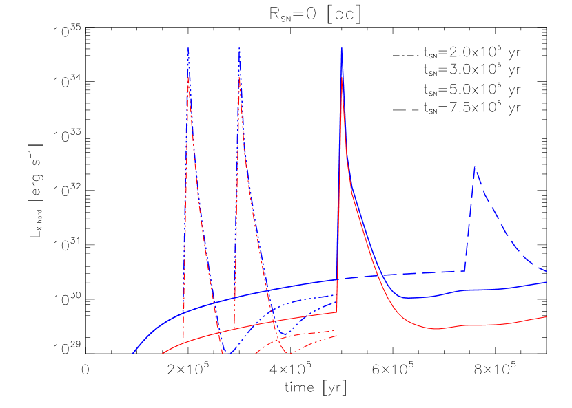
Figure 9: Same as Figure 5 for hard X-rays luminosities.

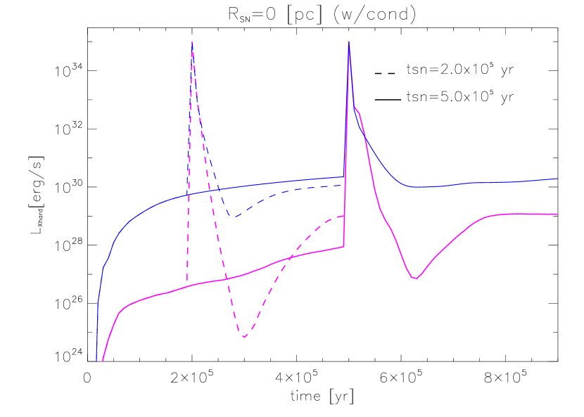
Figure 10: Same as Figure 6 for hard X-rays luminosities.

Figure 10 shows the evolution of the hard X-ray luminosity for the two models with thermal conduction and their counterpart without thermal conduction. The maximum luminosities and the time intervals of high hard X-ray emission are remarkably similar in spite of the thermal conduction. Although small differences can be seen, the position of the supernova explosion in the cluster does not have a significant influence in the overall and maximum thermal hard X-ray luminosity (see Figure 11).

Figure 11: Same as Figure 7 for hard X-rays luminosities.

It is also intresting to note that for an SN exploding at the centre of the cluster the highest luminosity achieved is much lower if the explosion occurs at later times (c.f. the long dashed curve in Figure 9 to the others).

The distribution of the hard X-ray emission before the SN explosion, at peak luminosity, and after the luminosity returns to its previous level can be seen as the (logarithmically spaced) contour levels in Figure 8. The emission during peak luminosity (middle row) is slightly more extended in the case where the SN is detonated off-centre (panel f), but returns to being concentrated inside the star cluster after the effect of the explosion has had time to decay (bottom row). The impact of thermal conduction on the hard X-ray emission is also evident. As can be seen, before (top row) or some time after (bottom row) the SN explosion the hard-band emission is at a much higher level in the cases without thermal conduction (left and right columns). However, during the luminosity peak (middle row) all models display important hard X-ray emission regardless of the inclusion of thermal conduction. The difference lies mainly in that in the case including thermal conduction (panel e) the emission is slightly more centralised than in the cases without.

We must note that the resolution used in the models is not enough to capture all the details of the flow. The use of higher resolution allows larger compression factors as well as more small scale structure inside the bubbles. To estimate the uncertainty in the X-ray luminosities due to poor resolution we have taken a test case (model sr0tsn5z0), and reproduce the setup in the Walicxe-3d code (Toledo-Roy et al., 2014). This code has adaptive mesh refinement (AMR), which allows to increase the resolution at a lower computational cost, but the thermal conduction is not fully implemented. We ran the test case at an equivalent resolution of $512^{3}$ and $1024^{3}$ cells, and while the details of the flow are different, the integrated X-ray luminosities seem to reach convergence. The peak luminosity in the higher resolution runs is a factor of $\sim 2$ larger than in the $256^{3}$ model sr0tsn5z0. And the times above $10^{34}$, $10^{35}~{}$, and $10^{36}~{}\mathrm{erg~{}s^{-1}}$ are larger by a factor of $\sim 1.5$. All the results presented above have an uncertainty of this order of magnitude due to the limited resolution.

4 Comparisons with observations

It is useful to compare our numerical models to the observations of particular superbubbles. We have thus turned our attention to four superbubbles located in the Large Magellanic Cloud (LMC): N70, N185, DEM L50 and DEM L152. These superbubbles have some particular features (as we will show) that make them compatible with our results.

N70 is a superbubble with a radius of approximately 53 pc. According to the observations there is a SN located closer to the center than the edge of the cluster. The X-ray luminosity reported by Reyes-Iturbide et al. (2014) is about 2.4($\pm 0.4$)$\times 10^{35}$ erg s^-1. We can see that our numerical results are in good agreement with these observations, in particular the models with the SN explosion in the center of the cluster.

The case of N185 is quite similar to that of N70. N185 has a spherical shape with an approximate radius of 43 pc (Oey, 1996). The X-ray luminosity obtained by Reyes-Iturbide et al. (2014) is 2.1 ($\pm 0.7$)$\times 10^{35}$ erg s^-1. Following Rosado et al. (1982), a possibility to explain the high velocity of this superbubble is that a SN explosion ocurred. From its spherical shape, we conclude that the SN explosion must be located near the centre of the cluster. As in the previous case, our numerical models are in good agreement with the observed X-ray luminosities.

Two other interesting cases are DEM L50 and DEM L152. These are two superbubbles with very intense X-ray emission. According to observations DM L152 has a radius of approximately 50 pc (Jaskot et al., 2011), and DEM L50 has roughly the same radius (Oey, 1996). Jaskot et al. (2011) reported an X-ray luminosity in the range 2.0-4.0$\times 10^{36}$ erg s^-1 for DEM L50 and an emission of 5.4-5.7$\times 10^{35}$ erg s^-1. These two superbubbles contrast with N70 and N185 in that they contain an off-centre SN explosion, which is clearly distinguishable in the observations. Only numerical model sn10tsn5zv predicts a luminosity comparable to the observed values. The luminosities predicted by other models are not high enough to match with these observed values.

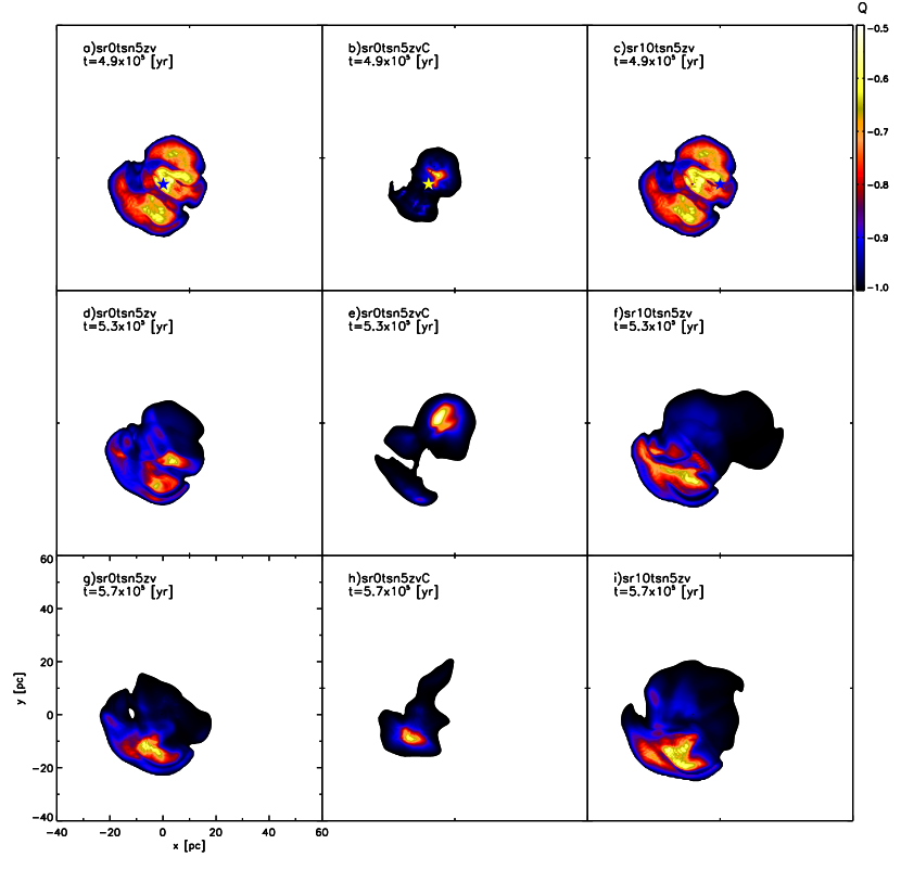
Figure 12: Hardness maps for the same cases shown in Figure 3.

In order to better compare with observations, we have calculated the hardness ratio for three of our models (see Figure 12). These models are those discussed in Section 3: two with a centred SN explosion that differ in the presence of thermal conduction, and the third with the SN explosion 10 pc off-centre. Following Jaskot et al. (2011), the hardness ratio is defined as:

$$Q=\frac{H-S}{H+S}\,,$$ (12)

where $H$ is the flux energy in the 2-10 keV energy band (corresponding to hard X-rays) and $S$ is the flux energy in the 0.1-2 keV energy band (corresponding to soft X-rays). After computing the fluxes and obtaining $Q$ for each cell in the simulation, we integrate along the $z$ axis in order to project the result into a 2D map, assuming that the X-ray absorption due to the material inside the bubble can be neglected.

In Figure 12 we observe that, before the SN explosion occurs, in models without thermal conduction (left and right columns) the hardness ratio peaks at $\sim-0.55$ at the centre of the stellar distribution, and decreases as we approach the edge of the cluster (the shell of swept-up ISM material emits mainly soft X-rays). In the case of the model that includes thermal conduction (middle column), we observe that $Q\sim-1.$ in most of the bubble, indicating that hard X-ray emission is largely negligible. As a result, the material ejected by the stars is cooled quickly from hard X-ray emitting temperatures ($10^{8}$ K) to temperatures in the range $10^{5}$ - $10^{6}$ K where soft X-ray emission is favored.

The SN explosion drastically alters the hardness maps for the models without thermal conduction. The SN shockwave sweeps the cluster volume, devoiding the center of the bubble of hard X-ray emitting gas and forming regions with $Q\sim-0.6$ closer to the edge of the bubble. In the model with thermal conduction, the hard X-ray emission is small to begin with, and the effect of the explosion on the hardness ratio is not as noticeable.

The predicted Q values obtained in our numerical models are similar to those obtained by Jaskot et al. (2011) for DEM L50 and DEM L152. Nevertheless, the specific details and assumptions of our simulations make it hard to establish direct comparisons to specific observed bubbles. In order to use the hardness ratio to predict some of the physical processes that occur or have occurred in the super-bubbles we would need to separately simulate the specific physical details, such as the position and mass and energy injection rates of each star, the ISM density, of each particular bubble, which is out of the scope of this work.

5 Conclusions

In this paper we present 3D hydrodynamical models of the evolution of the soft and hard thermal X-ray luminosities produced inside superbubbles driven by massive stellar winds including the effect of a supernova explosion and thermal conduction.

In all models we include the injection of mass and energy by a cluster of wind sources and a single SN event. We have varied the position of the SN with respect to the centre of the cluster as well as the detonation time. Also, we have worked out models with a uniform metallicity and models in which the environment, the winds and the SN have different metallicities. The metallicities are used to calculate the radiative cooling rate, and has an effect on the emissivity in X-rays. We have also taken into account the effects of thermal conduction in two of the models.

In the models with different metallicities we used $Z=0.3~{}Z_{\odot}$ for the environment, $3~{}Z_{\odot}$ for the winds and $10~{}Z_{\odot}$ for the SN ejecta. Our models show that the contribution of the metallicity of the winds and the supernova remnant is negligible for the soft X-ray emission of superbubbles, but becomes important for the hard X-ray component. In these models the ratio of soft to hard maximum luminosity can be as extreme as $10$ (i.e. the hard X-ray luminosity reaches 10% of the one for soft X-rays).

The models with thermal conduction result in a noticeable increase in the total luminosity of soft X-rays, by a factor of $\sim 1.25$. However, this factor is smaller than the two orders of magnitude difference predicted in the standard model of Weaver et al. (1977) and Chu & Mac Low (1990). The differences are likely to come from the fact that the standard model of Weaver et al. (1977) considers just a single star, and the extension to a star cluster in Chu & Mac Low (1990) and Chu et al. (1995) does not account for the cooling of the gas due to the interaction of the stellar winds. Thermal conduction has a slightly larger effect on the total integrated emission of hard X-rays, increasing the luminosity by a factor of $\sim 2.6$.

The most important contribution to the emission of soft and hard X-rays is produced by the injection of mass and energy by supernova explosions. In soft X-rays the luminosity increases by up to two orders of magnitude when we consider a supernova explosion placed at the cluster centre, and up to three orders when it explodes at the edge the star cluster.

Another important factor to consider is the time during which the luminosity remains high (i.e. observable). We show that when off-centre supernova events occur (close to the shell) the luminosity can increase by one or two orders of magnitude above that predicted by the standard model without SN, and that it can be maintained by a few tens of thousands of years. Indeed, as the supernova explosion occurs closer to the shell of swept up ISM, the maximum luminosity of soft X-rays as well as the time interval during which luminosity is enhanced increase.

An important increase in the maximum soft X-ray luminosity is produced when the SN ejecta collide with the dense shell of swept up ISM gas left behind by its interaction with the cluster wind. In these cases X-ray luminosities of $10^{36}$ erg s^-1 can be achieved. On the other hand, superbubbles where the SN explosions have not taken place near the shell, such as N 70 and N 185 (Jansen et al. 2011 and Reyes-Iturbide et al. 2014), have lower X-ray luminosity, and can be explained using our models with a slightly off-centre SN.

In clusters without SN events, or with a SN placed at the centre of the cluster, the contribution to the luminosity made by the SN is hard to observe, in particular because the observable flux increase in the soft X-ray emission lasts for a short time. This could be happening in massive stellar clusters in the Galaxy, such as Arches, Quintuplet and NGC 3603, that have a hundred massive stars with a total observed X-ray emission of $\sim 10^{34}$ erg s^-1.

References

- Añorve-Zeferino et al. (2009) Añorve-Zeferino, G. A., Tenorio-Tagle, G., & Silich, S. 2009, MNRAS, 394, 1284
- Cantó et al. (2000) Cantó, J., Raga, A.C. & Rodríguez, L.F., 2000, ApJ, 536, 896
- Chu et al. (1995) Chu, Y.-H., Chang, H.-W., Su, Y.-L. & Mac Low, M.-M., 1995, ApJ, 450, 157
- Chu & Mac Low (1990) Chu Y.-H. & Mac Low M.-M., 1990, ApJ, 365, 510
- Cowie & McKee (1997) Cowie L. L., & McKee C. F. 1977, ApJ, 211, 135
- Dere et al. (1997) Dere K. P., Landi E., Mason H. E., Monsignori Fossi B. C., Young P. R., 1997, A&AS, 125, 149
- Dunne et al. (2001) Dunne, B. C., Points, S. D., & Chu, Y.-H. 2001, ApJS, 136, 119
- Dunne et al. (2003) Dunne B. C., Chu Y.-H., Chen C.-H. R., Lowry J. D., Townsley L., Gruendl R. A., Guerrero M. A., Rosado M., 2003, ApJ, 590, 306
- Esquivel et al. (2009) Esquivel, A., Raga, A. C., Cantó, J. & Rodríguez González, A. 2009, AAP, 507, 855
- Harper-Clark & Murray (2009) Harper-Clark E.& Murray N. 2009, ApJ, 693, 1696
- Jansen et al. (2011) Jansen, F., Lumb, D., Altieri, B., et al. 2001, A&A, 365, L1
- Jaskot et al. (2011) Jaskot, A. E., Strickland, D. K., Oey, M. S., Chu, Y.-H., & García-Segura, G. 2011, ApJ, 729, 28
- Landi et al. (1996) Landi E., Del Zanna G., Young P. R., Dere K. P., Mason H. E., Landini M., 2006, ApJS, 162, 261
- Leitherer & Heckman (1995) Leitherer C., Heckman T. M., 1995, ApJS, 96, 9
- Maeder (1992) Maeder, A. 1992, A&A, 264, 105
- Mazzota et al. (1998) Mazzotta, P., Mazzitelli, G., Colafrancesco, S., & Vittorio, N. 1998, A&AS, 133, 403
- Oey (1995) Oey, M. S., & Massey, P. 1995, ApJ, 452, 210
- Oey (1996) Oey, M. S. 1996, ApJ, 467, 666
- Oey (2002) Oey, M. S., Groves, B., Staveley-Smith, L., & Smith, R. C. 2002,AJ, 123, 255
- Raga et al. (2009) Raga, A. C., Esquivel, A., Velázquez, P. F., et al. 2009, apjl, 707, L6
- Reyes-Iturbide et al. (2009) Reyes-Iturbide, J., Velázquez, P. F., Rosado, M. et al. 2009, MNRAS, 394, 1009
- Reyes-Iturbide et al. (2014) Reyes-Iturbide, J., Rosado, M., Rodríguez-González, A., Velázquez, P. F., Sánchez-Cruces, M. & Ambrocio-Cruz, P, 2014, ApJ, in press.
- Rodríguez-González et al. (2011) Rodríguez-González, A., Velázquez, P. F., Rosado, M., Esquivel, A., Reyes-Iturbide, J., Toledo-Roy, J. C., 2011, ApJ, 733, 34
- Rogers & Pittard (2014) Rogers, H. & Pittard, J.M, 2014, MNRAS, in press.
- Rosado et al. (1982) Rosado, M., Georgelin, Y. M., Georgelin, Y. P., Laval, A., & Monnet, G. 1982, A&A, 115, 61
- Silich et al. (2001) Silich, S., Tenorio-Tagle, G., Terlevich, R., Terlevich, E. & Netzer, H., 2001, MNRAS, 324, 191
- Silich et al. (2004) Silich, S., Tenorio-Tagle, G., & Rodríguez-González, A. 2004, ApJ, 610, 226
- Spitzer (1962) Spitzer, L., Jr, 1962, Physics of Fully Ionized Gases. Wiley Interscience, New York
- Stevens & Hartwell (2003) Stevens, I. R. & Hartwell, J. M., 2003, MNRAS, 339, 280
- Toledo-Roy et al. (2014) Toledo-Roy, J. C., Esquivel, A., Velázquez, P. F., & Reynoso, E. M. 2014, MNRAS, 442, 229
- Toro et al. (1994) Toro, E. F., Spruce, M., & Speares, W. 1994, Shock Waves, 4, 25
- Velázquez et al. (2013) Velázquez, P. F., Rodríguez-González, A., Esquivel, A., Rosado, M. & Reyes-Iturbide, J., 2013, ApJ, 767, 69
- Weaver et al. (1977) Weaver, R., McCray, R., Castor, J., Shapiro, P. & Moore, R., 1977, ApJ, 218, 377