Towards A Theory Of Quantum Computability

Abstract.

We propose a definition of quantum computable functions as mappings between superpositions of natural numbers to probability distributions of natural numbers. Each function is obtained as a limit of an infinite computation of a quantum Turing machine. The class of quantum computable functions is recursively enumerable, thus opening the door to a quantum computability theory which may follow some of the classical developments.

1. Introduction

Despite the availability of a large corpus of results, quantum computability still lacks a general treatment akin to classical computability theory. Taking as a reference model (quantum) Turing machines, one of the main obstacles is that while it is obvious how to understand a classical Turing machine (TM) as a device computing a numerical function, the same is not so for a quantum Turing machine (QTM).

In a naïve, but suggestive way, a QTM may be described as a classical TM which, at any point of its computation, evolves into several different classical configurations, each characterised by a complex amplitude. Such different configurations should be imagined as simultaneously present, “in superposition”—a simultaneity formally expressed as a weighted sum $\sum d_{i}\mathsf{C}_{i}$ of classical configurations $C_{i}$, with complex coefficients $d_{i}$. Even when starting from a classical configuration, in a QTM, there is not a single result, but a superposition from which we can read off several numerical “results” with certain probabilities. Moreover, QTMs never have genuinely finite computations and one should therefore find a way to define when and how a result can be read off.

In this paper we propose a notion of “function computable by a quantum Turing machine,” as a mapping between superpositions of initial classical configurations to probability distributions of natural numbers, which are obtained (in general) as a limit of an infinite QTM computation.

Before reaching this point, however, we must go back to the basics, and look to the very notion of QTM. Because, if it is true that configurations of a QTM are superpositions $\sum d_{i}\mathsf{C}_{i}$ of classical configurations, quantum physics principles impose severe constraints on the possible evolutions of such machines. First, in any superposition $\sum d_{i}\mathsf{C}_{i}$, we must have $\sum|d_{i}|^{2}=1$. Second, there cannot be any finite computation—we may of course name a state as “final” and imagine that we read the result of the computation (whatever this means) when the QTM enters such a state, but we must cope with the fact that the computation will go on afterwards. Moreover, since any computation of a QTM must be reversible [2], in the sense that the operator describing the evolution of the QTM must be invertible, we cannot neither force the machine to loop on its final configuration. On the other hand, because of reversibility, even the initial configuration must have a predecessor. Summing up, an immediate consequence of all the above considerations is that every state must have at least one incoming and one outgoing transition and that such transitions must accord to several constraints forced by quantum physics principles. In particular, transitions must enter the initial state—since a priori it might be reached as the evolution from a preceding configuration — and exit the final state—allowing the machine configuration to evolve even after it has reached the final result.

The reversibility physical constraints are technically expressed by the requirement that the evolution operator of a QTM be unitary. If we now want to use a QTM to compute some result, we are still faced with the problem of when (and how, but for the moment let’s postpone this) reading such a final result, given that the computation evolves also from the final state, and that, without further constraints, it might of course evolve in many, different possible ways. Bernstein and Vazirani in their seminal paper [3] (from now on we shall refer to this paper as “B&​V”) first define (non unitary) QTMs; select then the “well-formed” QTMs as the unitary-operator ones; and define finally “well-behaved” QTMs as those which produce a superposition in which all classical configurations are simultaneously (and for the first time) in the final state. What happens after this moment, it is not the concern of B&​V.

Our goal is to relax the requirement of simultaneous “termination”, allowing meaningful computations to reach superpositions in which some classical configurations are final (and give a “result”), and some are not. Those which are not final, should be allowed to continue the computation, possibly reaching a final state later. The “final result” will then be defined as a limit of this process. In order to assure that at every step of the computation the superposition of the final configurations is a valid approximation of the limit result, we must guarantee that once a final state is entered, the “result” that we read off is not altered by the further (necessary, by unitarity) evolution. To obtain this, we restrict the transition function out of a final state, without violating unitarity. We obtain this goal by “marking” the symbols on the tape—once a final state is entered, the machine remains in that final state, replaces the symbol $a$ under the head with the same marked symbol $\overline{a}$, and moves to the right. Dually (to preserve unitarity), when the machine is in an initial state, it may rollback to another initial configuration in which the symbol $a$ to the left of the head is replaced by the marked symbol $\overline{a}$ and the head is on it; that is, looking at the corresponding forward transition, when in the initial state, if the machine head reads a marked $\overline{a}$, then the machine remains in that initial state, replaces the symbol with the unmarked $a$, and moves to the right. The role of the extra marked symbols is restricted to these “final” and “initial” evolutions. In particular, there are no transitions out of a final state when reading a marked symbol, or which enter an initial state writing a marked symbol, and no transitions at all—involving marked symbols—entering or exiting a state that is neither final nor initial. That these machines correctly induce a unitary operator is the content of Theorem 7. In the following, marked symbols will be called the extra symbols and we will generalise this discussion from a final (initial) state to a set of target (source) states.

After the definition of QTMs and of the corresponding functions, we will discuss their expressive power, comparing them to the QTMs studied in the literature. The QTMs of B&​V form a robust class, but meaningful computations are defined only for classical inputs (a single natural number with amplitude 1). Moreover, their QTMs “terminate” synchronously—either all paths in superpositions enter a final state at the same time, or all of them diverge. As a consequence, there is no chance to study—and give meaning—to infinite computations. More important, the class of “sensible” QTMs (in B&​V’s terminology: the well-formed, well-behaved, normal form QTMs) is not recursively enumerable, since the constraint of “simultaneous termination” is undecidable.

In Deutsch’s original proposal [10], any quantum TM has an explicit termination bit which the machine sets when entering a final configuration. While it is guaranteed that final probabilities are preserved, the observation protocol requires that one checks termination at every step, since the machine may well leave the final state (and change the tape). Deutsch’s machines could in principle be used to define meaningful infinite computations, but we know of no such an attempt.

In our analysis: (i) there is no termination bit: a quantum configuration is a genuine superposition of classical configurations; (ii) any computation path (that is, any element of the superposition) evolves independently from the others: any path may terminate at its own time, or may diverge; (iii) infinite computations are meaningful; (iv) we may observe the result of the computation in a way akin to Deutsch’s one, but with the guarantee that once a final state is entered, the machine will not change the corresponding “result” during a subsequent computation; (v) the class of QTMs is recursively enumerable, thus opening the door to a quantum computability theory which may follow some of the classical developments.

2. Quantum Turing Machines

In this section we define quantum Turing machines. We assume the reader be familiar with classical Turing machines (in case, see [9]).

In all the paper we shall assume that the tape alphabet $\Sigma$ is finite and contains at least the symbols $1$ and $\Box$: $1$ will be used to code natural numbers in unary notation; $\Box$ will be the blank symbol. For any $n\in\mathbb{N}$, $\underline{n}$ will denote the string $1^{n+1}$. The greek letters $\alpha,\beta$, eventually indexed, will denote strings in $\Sigma^{*}$; $\lambda$ will denote the empty string; $\alpha\beta$ will denote the concatenation of $\alpha$ and $\beta$.

2.1. QTM

Given a tape alphabet $\Sigma$, we associate an extra tape symbol $\overline{a}$ to any $a\in\Sigma$ (including the blank $\Box$); $\overline{\Sigma}=\{\overline{a}\mid a\in\Sigma\}$ is the extra tape alphabet. Finally, $\widehat{\Sigma}=\Sigma\cup\overline{\Sigma}$. As we discussed in the introduction, extra tape symbols will only appear in computations involving initial or final states.

As in B&​V, we assume that a machine move always implies a displacement of the machine head, to the left ($L$) or the right ($R$) on the tape; $\mathbb{D}=\{L,R\}$ is the set of the displacements.

For $I$ denumerable, $\ell^{2}(I)$ is the Hilbert space of square summable, $I$-indexed sequences of complex numbers

$$\left\{\phi:I\rightarrow\mathbb{C}\mid\sum_{C\in I}|\phi(C)|^{2}<\infty\right\},$$

equipped with an inner product $\left\langle\mathsf{.}\mid\mathsf{.}\right\rangle$ and the euclidean norm $\left\|\phi\right\|=\sqrt{\left\langle\mathsf{\phi}\mid\mathsf{\phi}\right\rangle}$. See Appendix A for more details.

Definition 1 (Quantum Turing machines).

Given a finite set of states $\mathcal{Q}$ and an alphabet $\Sigma$, a Quantum Turing Machine (QTM) is a tuple

$$M=\langle\Sigma,\mathcal{Q},\mathcal{Q}_{s},\mathcal{Q}_{t},\delta,q_{i},q_{f}\rangle$$

where

• $\mathcal{Q}_{s}\subseteq\mathcal{Q}$ is the set of source states of $M$, and $q_{i}\in\mathcal{Q}_{s}$ is a distinguished source state named the initial state of $M$;

• $\mathcal{Q}_{t}\subseteq\mathcal{Q}$ is the set of target states of $M$, and $q_{f}\in\mathcal{Q}_{t}$ is a distinguished target state named the final state of $M$;

• if we define $\mathcal{Q}_{0}=\mathcal{Q}\setminus(\mathcal{Q}_{s}\cup\mathcal{Q}_{t})$, then $\delta=\delta_{0}\cup\delta_{s}\cup\delta_{t}$ is the quantum transition function of $M$, defined as the union of the following three functions with disjoint domains:

  $$\delta_{0} :((\mathcal{Q}_{0}\cup\mathcal{Q}_{s})\times\Sigma)\to\ell^{2}((\mathcal{Q}_{0}\cup\mathcal{Q}_{t})\times\Sigma\times\mathbb{D})$$

  $$\delta_{s} :(\mathcal{Q}_{s}\times\overline{\Sigma})\to\ell^{2}(\mathcal{Q}_{s}\times\Sigma\times\mathbb{D})$$

  $$\delta_{t} :(\mathcal{Q}_{t}\times\Sigma)\to\ell^{2}(\mathcal{Q}_{t}\times\overline{\Sigma}\times\mathbb{D})$$

• the source transition function $\delta_{s}$ is defined by

  $$\delta_{s}(q_{s},\overline{a})(q_{s}^{\prime},b,d)=\begin{cases}1&\mbox{if $(q_{s}^{\prime},b,d)=(q_{s},a,R)$}\\ 0&\mbox{otherwise}\end{cases}$$

  for every $(q_{s},\overline{a})\in\mathcal{Q}_{s}\times\overline{\Sigma}$ and every $(q_{s}^{\prime},b,d)\in\mathcal{Q}_{s}\times\Sigma\times\mathbb{D}$

• the target transition function $\delta_{t}$ is defined by

  $$\delta_{t}(q_{t},a)(q_{t}^{\prime},\overline{b},d)=\begin{cases}1&\mbox{if $(q_{t}^{\prime},\overline{b},d)=(q_{t},\overline{a},R)$}\\ 0&\mbox{otherwise}\end{cases}$$

  for every $(q_{t},a)\in\mathcal{Q}\times\Sigma$ and every $(q_{t}^{\prime},\overline{b},d)\in\mathcal{Q}_{t}\times\overline{\Sigma}\times\mathbb{D}$

• the main transition function $\delta_{0}$ satisfies the following local unitary conditions

  1. for any $(q,a)\in(\mathcal{Q}_{0}\cup\mathcal{Q}_{s})\times\Sigma$

     $$\sum_{(p,b,d)\in(\mathcal{Q}_{0}\cup\mathcal{Q}_{t})\times\Sigma\times\mathbb{D}}|\delta_{0}(q,a)(p,b,d)|^{2}=1$$

  2. for any $(q,a),(q^{\prime},a^{\prime})\in(\mathcal{Q}_{0}\cup\mathcal{Q}_{s})\times\Sigma$ with $(q,a)\neq(q^{\prime},a^{\prime})$
     

     $${\sum_{(p,b,d)\in(\mathcal{Q}_{0}\cup\mathcal{Q}_{t})\times\Sigma\times\mathbb{D}}\delta_{0}(q^{\prime},a^{\prime})(p,b,d)^{*}\delta_{0}(q,a)(p,b,d)=0}$$

  3. for any $(q,a,b),(q^{\prime},a^{\prime},b^{\prime})\in(\mathcal{Q}_{0}\cup\mathcal{Q}_{s})\times\Sigma^{2}$
     

     $${\sum_{p\in(\mathcal{Q}_{0}\cup\mathcal{Q}_{t})}\delta_{0}(q^{\prime},a^{\prime})(p,b^{\prime},L)^{*}\delta_{0}(q,a)(p,b,R)=0}$$

We remark that the domains and codomains of the three transition functions $\delta_{0}$, $\delta_{s}$ and $\delta_{t}$ are disjoint. Indeed, if we define

$$\mathcal{S}_{0} =(\mathcal{Q}_{0}\cup\mathcal{Q}_{s})\times\Sigma \mathcal{S}_{s} =\mathcal{Q}_{s}\times\overline{\Sigma} \mathcal{S}_{t} =\mathcal{Q}_{t}\times\Sigma$$

$$\mathcal{T}_{0} =(\mathcal{Q}_{0}\cup\mathcal{Q}_{t})\times\Sigma \mathcal{T}_{s} =\mathcal{Q}_{s}\times\Sigma \mathcal{T}_{t} =\mathcal{Q}_{t}\times\overline{\Sigma}$$

we can then write, in a compact way

$$\delta_{x}=\mathcal{S}_{x}\to\ell^{2}(\mathcal{T}_{x}\times\mathbb{D})\qquad\qquad\mbox{for $x\in\{0,s,t\}$}$$

and see that, for $x,y\in\{0,s,t\}$,

$$\mathcal{S}_{x}\cap\mathcal{S}_{y}=\emptyset\qquad\qquad\qquad\mathcal{T}_{x}\cap\mathcal{T}_{y}=\emptyset$$

when $x\neq y$.

2.2. Configurations

A configuration of a (classical) TM is a triple formed by the content of the tape, the state of the machine and the position of the tape head. As usual, we assume that only a finite portion of the tape contains non-blank symbols. We may therefore represent such a configuration as a triple $\langle\alpha,q,\beta\rangle\in\widehat{\Sigma}^{*}\times\mathcal{Q}\times\widehat{\Sigma}^{*}$ where:

1. $q$ is the current state;

2. $\beta$ is the right content of the tape and its first symbol is the one under the head (we say also: in the current cell). That is, $\beta=u\beta^{\prime}$, where the current symbol $u$ is the content of the current cell (i.e. the one pointed by the tape head) and $\beta^{\prime}$ is the longest string on the tape ending with a symbol different from $\Box$ and whose first symbol (if any) is written in the cell immediately to the right of the current cell; by convention, when the current cell and all the right content of the tape is empty, we shall also write $\langle\alpha,q,\lambda\rangle$ instead of $\langle\alpha,q,\Box\rangle$;

3. $\alpha$ is the left content of the tape. That is, it is either the empty string $\lambda$, or it is the longest string on the tape starting with a symbol different from $\Box$, and whose last symbol is written in the cell immediately to the left of the current cell.

According to this definition, in a configuration $\langle\alpha,q,\beta\rangle$ the string $\alpha$ does not start with a blank $\Box$, and $\beta$ does not end with a blank. In the following it will be useful to manipulate configurations which are extended with blanks to the right (of the right content) or to the left (of the left content). For this, we equate configurations up to the three equivalence relations induced by the following equations

$$\alpha\simeq_{l}\Box\alpha\qquad\qquad\beta\simeq_{r}\beta\Box$$

$$\langle\alpha,q,\beta\rangle\simeq\langle\alpha^{\prime},q,\beta^{\prime}\rangle\qquad\qquad\mbox{when $\alpha\simeq_{l}\alpha^{\prime}$ and $\beta\simeq_{r}\beta^{\prime}$}$$

We now turn to QTMs. Observe first that while cells containing the blank symbol $\Box$ are considered empty, cells containing the extra symbol $\overline{\Box}$ are not empty and should not be ignored on the left/right side of the tape. Moreover, in view of the particular evolution required for source/target states, and the special role of extra symbols, some of the triples $\langle\alpha,q,\beta\rangle$ cannot occur as actual configurations in a computation of a QTM. We limit our QTMs to configurations where extra symbols appear in $\alpha\beta$ only when the current state is a source (target) state and, moreover all the extra symbols are immediately to the right (left) of the tape head.

Definition 2 (configurations).

Let $M=(\Sigma,\mathcal{Q},\mathcal{Q}_{s},\mathcal{Q}_{t},\delta,q_{0},q_{f})$ be a QTM. A configuration of $M$ is a triple $\langle\alpha,q,\beta\rangle\in\widehat{\Sigma}^{*}\times\mathcal{Q}\times\widehat{\Sigma}^{*}$ s.t.

1. if $q\not\in\mathcal{Q}_{s}\cup\mathcal{Q}_{t}$, then $\alpha\beta\in\Sigma^{*}$, that is, the tape does not contain extra symbols;

2. if $q\in\mathcal{Q}_{s}$, then $\alpha\in\Sigma^{*}$ and $\beta\in\overline{\Sigma}^{*}\Sigma^{*}$;

3. dually, if $q\in\mathcal{Q}_{t}$, then $\beta\in\Sigma^{*}$ and $\alpha\in\Sigma^{*}\overline{\Sigma}^{*}$.

The set of configurations of $M$ is denoted by $\mathfrak{C}_{M}$. A configuration of $M$ is a source/target configuration when the corresponding state is a source/target state, moreover, it is a final/initial configuration when the current state is final/initial. By $\mathfrak{F}_{M}$ we shall denote the set of the final configurations of $M$.

In the following, the index $M$ in $\mathfrak{C}_{M}$ and in the other names indexed by the machine might drop when clear from the context.

2.3. Quantum configurations

As already discussed in the introduction, the evolution of a QTM is described by superpositions of configurations (as defined in Definition 2). If $\mathcal{B}\subseteq\mathfrak{C}_{M}$ is a set of configurations, superpositions are elements of the Hilbert space $\ell^{2}(\mathcal{B})$ (see, e.g., [4, 17]). Quantum configurations of a QTM $M$ are those elements of $\ell^{2}(\mathfrak{C}_{M})$ with unitary norm. We remark that, since there is no bound on the size of the tape in a configuration, the Hilbert space of the configurations must be infinite dimensional.

Definition 3 (quantum configurations).

Let $M$ be a QTM. The elements of the set $\mathfrak{q}\mathfrak{C}_{M}=\{\phi\in\ell^{2}(\mathfrak{C}_{M})\mid\sum_{C\in\mathfrak{C}_{M}}|\phi(C)|^{2}=1\}$ are the q-configurations (quantum configurations) of $M$.

We shall use Dirac notation (see Appendix A) for the elements $\phi,\psi$ of $\mathfrak{q}\mathfrak{C}_{M}$, writing them $\left|\mathsf{\phi}\right\rangle,\left|\mathsf{\psi}\right\rangle$.

Definition 4.

For any set of configurations $\mathcal{B}\subseteq\mathfrak{C}_{M}$ and any $C\in\mathcal{B}$ let $\left|\mathsf{C}\right\rangle:\mathcal{B}\to\mathbb{C}$ be the function

$$\left|\mathsf{C}\right\rangle(D)=\left\{\begin{array}[]{ll}1&\mbox{if}\;C=D\\ 0&\mbox{if}\;C\neq D.\end{array}\right.$$

The set $\mathsf{CB}(\mathcal{B})$ of all such functions is a Hilbert basis for $\ell^{2}(\mathcal{B})$ (see, e.g., [15]). In particular, following the literature on quantum computing, $\mathsf{CB}(\mathfrak{C}_{M})$ is called the computational basis of $\ell^{2}(\mathfrak{C})$. Each element of the computational basis is called base q-configuration.

With a little abuse of language we shall write $\left|\mathsf{C}\right\rangle\in\left|\mathsf{\phi}\right\rangle$ when $\phi(C)\neq 0$. The span of $\mathsf{CB}(\mathcal{B})$, denoted by $\mathsf{span}(\mathsf{CB}(\mathcal{B}))$, is the set of the finite linear combinations with complex coefficients of elements of $\mathsf{CB}(\mathcal{B})$; $\mathsf{span}(\mathcal{B})$ is not a Hilbert space, although $\ell^{2}(\mathcal{B})$ is the (unique, up to isomorphism) completion of $\mathsf{span}(\mathcal{B})$. Moreover, each unitary operator $U$ on $\mathsf{span}(\mathcal{B})$ has a unique unitary extension on $\ell^{2}(\mathcal{B})$ [3].

For a list of the main definitions, properties and notations on Hilbert spaces with denumerable basis, see Appendix A. In particular, subsection A.1 presents a synoptic table of the so-called Dirac notation that we shall use in the paper.

2.4. Time evolution operator

For any QTM $M$ with alphabet $\Sigma$, and space of states $\mathcal{Q}$, the step function $\gamma_{M}:\mathfrak{C}_{M}\times\mathcal{Q}\times\widehat{\Sigma}\times\mathbb{D}\to\mathfrak{C}_{M}$ is the map that, given a configuration of the tape and a triple $(p,b,d)$ describing a “classical” step of a Turing machine, replaces the symbol in the current cell with the symbol $p$, moves the head on the $d$ direction, and sets the machine into the new state $p$. Formally:

$$\gamma_{M}(\langle\alpha w,q,u\beta\rangle,p,v,d)\simeq\begin{cases}\langle\alpha wv,p,\beta\rangle&\mbox{when $d=R$}\\ \langle\alpha,p,wv\beta\rangle&\mbox{when $d=L$.}\end{cases}$$

The evolution of a QTM $M=\langle\mathcal{Q},\Sigma,\delta,q_{0},q_{f}\rangle$ can then be defined as a map on q-configurations. Following the three-parts definition of the transition function, let

$$\mathfrak{C}^{x}_{M}=\{\langle\alpha,q,u\beta\rangle\in\mathfrak{C}_{M}\mid(q,u)\in\mathcal{S}_{x}\}\qquad\qquad\mbox{with $x\in\{0,s,t\}.$}$$

It is easily seen that $\mathfrak{C}^{0}_{M}$, $\mathfrak{C}^{s}_{M}$, and $\mathfrak{C}^{t}_{M}$ are a partition of $\mathfrak{C}_{M}$ (they are pairwise disjoint, because $\mathcal{S}_{0}$, $\mathcal{S}_{s}$, and $\mathcal{S}_{t}$ are pairwise disjoint). Therefore, given

$$C=\langle\alpha,q,u\beta\rangle\in\mathfrak{C}_{M}\qquad\qquad C_{p,v,d}=\gamma_{M}(C,p,v,d)$$

we can define

$$W_{M}(\left|\mathsf{C}\right\rangle)=\sum_{(p,v,d)\in\mathcal{T}_{x}\times\mathbb{D}}\delta_{x}(q,u)(p,v,d)\,\left|\mathsf{C_{p,v,d}}\right\rangle\qquad\mbox{when $C\in\mathfrak{C}^{x}_{M}$.}$$

Proposition 5.

$W_{M}(\left|\mathsf{C}\right\rangle)\in\mathsf{span}(\mathsf{CB}(\mathfrak{C}))$, for any $C\in\mathfrak{C}$. Then, $W_{M}$ naturally extends to an automorphism on the linear space of q-configurations

$$W_{M}:\mathsf{span}(\mathsf{CB}(\mathfrak{C}))\to\mathsf{span}(\mathsf{CB}(\mathfrak{C})).$$

Proof.

Let $C$ and $C_{p,v,d}$ be as in the definition of $W_{M}$.

1. Let $C\in\mathfrak{C}^{0}_{M}$. If $(p,v)\in\mathcal{T}_{0}$, then $C_{p,v,d}\in\mathfrak{C}^{t}_{M}$ when $p\in\mathcal{Q}_{t}$, and $C_{p,v,d}\in\mathfrak{C}^{0}_{M}$ otherwise. Thus, $C_{p,v,d}\in\mathfrak{C}_{M}$, for every $(p,v,d)\in\mathcal{T}_{0}\times\mathbb{D}$.

2. Let $C\in\mathfrak{C}^{s}_{M}$, that is, $u=\overline{a}$ for some $a\in\Sigma$ and $C=\langle\alpha,q,\overline{a}\overline{\gamma}\beta\rangle$, where $\alpha,\beta,\gamma\in\Sigma^{*}$. If $(p,v)\in\mathcal{T}_{s}$, then $\delta(q,\overline{a})(p,v,d)\neq 0$ iff $v=a$ and $d=R$, namely, $W_{M}(\left|\mathsf{C}\right\rangle)=\left|\mathsf{C_{p,a,R}}\right\rangle$ with $C_{p,a,R}=\langle\alpha a,p,\overline{\gamma}\beta\rangle$. Then, if the symbol $\overline{a}$ replaced by $a$ was the last extra symbol on the tape, that is $\gamma=\lambda$, then $C_{p,a,R}\in\mathfrak{C}^{0}_{M}$, otherwise $C_{p,a,R}\in\mathfrak{C}^{s}_{M}$. In any case, $W_{M}(\left|\mathsf{C}\right\rangle)\in\mathsf{span}(\mathsf{CB}(\mathfrak{C}))$.

3. Let $C\in\mathfrak{C}^{t}_{M}$, that is, $u=a$ for some $a\in\Sigma$ and $C=\langle\alpha\overline{\gamma},q,\beta\rangle$, where $\alpha,\beta,\gamma\in\Sigma^{*}$. If $(p,v)\in\mathcal{T}_{t}$, then $\delta(q,a)(p,v,d)\neq 0$ iff $v=\overline{a}$ and $d=R$; namely, $W_{M}(\left|\mathsf{C}\right\rangle)=\left|\mathsf{C_{p,\overline{a},R}}\right\rangle$ with $C_{p,\overline{a},R}=\langle\alpha\overline{\gamma}\overline{a},p,\beta\rangle$. Then, $C_{p,a,R}\in\mathfrak{C}^{t}_{M}$ and $W_{M}(\left|\mathsf{C}\right\rangle)\in\mathsf{span}(\mathsf{CB}(\mathfrak{C}))$.

Summing up, $W_{M}(\left|\mathsf{C}\right\rangle)\in\mathsf{span}(\mathsf{CB}(\mathfrak{C}))$ in any case. Thus, $W_{M}$ uniquely extends to an automorphism on $\mathsf{span}(\mathsf{CB}(\mathfrak{C}))$ by linearity: that is

$$W_{M}(\sum_{C\in\mathfrak{C}_{M}}k_{C}\left|\mathsf{C}\right\rangle)=\sum_{C\in\mathfrak{C}_{M}}k_{C}W_{M}(\left|\mathsf{C}\right\rangle).$$

∎

By completion, $W_{M}$ extends in a unique way to an operator on the Hilbert space of q-configurations.

Definition 6 (time evolution operator).

The time evolution operator of $M$ is the unique extension

$$U_{M}:\ell^{2}(\mathfrak{C}_{M})\to\ell^{2}(\mathfrak{C}_{M})$$

of the linear operator $W_{M}:\mathsf{span}(\mathsf{CB}(\mathfrak{C}))\to\mathsf{span}(\mathsf{CB}(\mathfrak{C}))$.

Theorem 7.

The time evolution operator of a QTM is unitary.

Proof.

The proof is a variant of the one given by B&​V and by Nishimura and Ozawa [16]. In particular, we prove first that $U_{M}$ is an isometry of $\ell^{2}(\mathfrak{C})$, and then that, in this particular case, this implies that $U_{M}$ is unitary (which, in general, holds for finite dimensional Hilbert spaces only—in the infinite dimensional case an isometry might not be surjective). The full details of the proof are given in Appendix B. ∎

In Appendix B we shall not only show that the unitary local conditions imply the unitarity of the time evolution operator (i.e., Theorem 7), but that they are also necessary. We remark that, this is not just a simple adaptation to our case of the already known proofs for B&​V QTM; in fact, we also simplify the argument that allows to show that the isometry of $U_{M}$ implies its unitarity.

Since the time evolution operator of a QTM is unitary, it preserves the norm of its argument, hence it maps q-configurations into q-configurations.

Proposition 8.

Let $M$ be a QTM. If $\left|\mathsf{\phi}\right\rangle\in\mathfrak{q}\mathfrak{C}$, then $U_{M}\left|\mathsf{\phi}\right\rangle\in\mathfrak{q}\mathfrak{C}$.

Definition 9 (initial and final configurations).

A q-configuration $\left|\mathsf{\phi}\right\rangle=\sum_{i}e_{i}\left|\mathsf{C_{i}}\right\rangle$ is initial if all the $C_{i}$ are initial, and it is final if all the $C_{i}$ are final. Moreover, $\mathfrak{q}\mathfrak{F}$ is the set of final q-configurations, and we shall denote by $\left|\mathsf{\underline{n}}\right\rangle$ the initial configuration $\langle\lambda,q_{0},\underline{n}\rangle$.

Definition 10 (computations).

Let $M$ be a QTM and let $U_{M}$ be its time evolution operator. For an initial q-configuration $\left|\mathsf{\phi}\right\rangle$, the computation of $M$ on $\left|\mathsf{\phi}\right\rangle$ is the denumerable sequence $\{\left|\mathsf{\phi_{i}}\right\rangle\}_{i\in\mathbb{N}}$ s.t.

1. $\left|\mathsf{\phi_{0}}\right\rangle=\left|\mathsf{\phi}\right\rangle$;

2. $\left|\mathsf{\phi_{i}}\right\rangle=U_{M}^{i}\left|\mathsf{\phi}\right\rangle$.

Clearly, any computation of a QTM $M$ is univocally determined by its initial q-configuration. The computation of $M$ on initial q-configuration $\left|\mathsf{\phi}\right\rangle$ will be denoted by $K_{\left|\mathsf{\phi}\right\rangle}^{M}$.

Lemma 11.

Let $C\in\mathfrak{F}$ be a final configuration without extra symbols; in particular, let $C=\langle\beta,q_{f},\alpha\rangle$ with $\alpha\beta\in\Sigma^{*}$ and $\alpha=a_{1}\ldots a_{l}$. For every $k\geq 0$, let

$$C[k]=\begin{cases}\langle\beta,q_{f},\overline{a}_{1}\ldots\overline{a}_{k}a_{k+1}\ldots a_{l}\rangle&\quad\mbox{for }0\leq k<l\\ \langle\beta,q_{f},\overline{a}_{1}\ldots\overline{a}_{l}\overline{\Box}^{k-l}\rangle&\quad\mbox{otherwise}\end{cases}$$

that is, for $k>0$, $C[k]$ is obtained from $C$ by replacing the current symbols and the first $k-1$ symbols to its right by the corresponding extra symbols.

1. $\left|\mathsf{C[j]}\right\rangle=U_{M}^{j-i}\left|\mathsf{C[i]}\right\rangle$, for every $i,j\geq 0$. More generally, for every $i,j\geq 0$ and every $\phi\in\mathfrak{q}\mathfrak{C}$,

   $$\left\langle U^{j-i}_{M}\left|\mathsf{\phi}\right\rangle,\left|\mathsf{C[j]}\right\rangle\right\rangle=\left\langle\mathsf{\phi}\mid\mathsf{C[i]}\right\rangle$$

2. $U_{M}^{-j-i}\left|\mathsf{C[i]}\right\rangle\in\ell^{2}(\mathfrak{C}\setminus\mathfrak{F})$, for every $i\geq 0$ and $j>0$.

3. Let $\left|\mathsf{\phi}\right\rangle\in\ell^{2}(\mathfrak{C}\setminus\mathfrak{F})$. For every $i,j\geq 0$, we have that:

   1. $\left|\mathsf{C[i]}\right\rangle\in U^{j}\left|\mathsf{\phi}\right\rangle$ only if $i<j$.

   2. $\left|\mathsf{C[i]}\right\rangle\not\in U^{-j}\left|\mathsf{\phi}\right\rangle$, that is, $U^{-j}\left|\mathsf{\phi}\right\rangle\in\ell^{2}(\mathfrak{C}\setminus\mathfrak{F})$

Proof.

1. By the definition of the transition function, we can easily see that $\left|\mathsf{C[i+1]}\right\rangle=U_{M}\left|\mathsf{C[i]}\right\rangle$, for every $i\geq 0$. Therefore, $\left|\mathsf{C[j]}\right\rangle=U_{M}^{j}\left|\mathsf{C[0]}\right\rangle=U_{M}^{j-i}U_{M}^{i}\left|\mathsf{C[0]}\right\rangle=U_{M}^{j-i}\left|\mathsf{C[i]}\right\rangle$, for every $i,j\geq 0$. Then, since $U_{M}$ is unitary, $\left\langle U^{j-i}_{M}\left|\mathsf{\phi}\right\rangle,\left|\mathsf{C[j]}\right\rangle\right\rangle=\left\langle\mathsf{\phi}\right|U^{i-j}_{M}\left|\mathsf{C[j]}\right\rangle=\left\langle\mathsf{\phi}\mid\mathsf{C[i]}\right\rangle$.

2. Let $D$ be any final configuration without extra symbols. By the previous item, $\left\langle U^{-j-i}_{M}\left|\mathsf{C[i]}\right\rangle,\left|\mathsf{D[k]}\right\rangle\right\rangle=\left\langle\mathsf{C[i]}\mid\mathsf{D[k+j+i]}\right\rangle=0$, for every $k\geq 0$, since $j>0$ and then $k+j+i>i$. Therefore, since $D[k]\not\in U^{-j-i}_{M}\left|\mathsf{C[i]}\right\rangle$, for any $D$ and any $k$, we conclude that $U_{M}^{-j-i}\left|\mathsf{C[i]}\right\rangle\in\ell^{2}(\mathfrak{C}\setminus\mathfrak{F})$.

3. They are immediate consequences of the previous two items. Indeed, $\left\langle U^{j}_{M}\left|\mathsf{\phi}\right\rangle,\left|\mathsf{C[i]}\right\rangle\right\rangle=\left\langle\mathsf{\phi}\mid\mathsf{C[i-j]]}\right\rangle=0$ for $i\geq j$, and $\left\langle U^{-j}_{M}\left|\mathsf{\phi}\right\rangle,\left|\mathsf{C[i]}\right\rangle\right\rangle=\left\langle\mathsf{\phi}\mid\mathsf{C[i+j]]}\right\rangle=0$, for $j\geq 0$, since $\left|\mathsf{\phi}\right\rangle\in\ell^{2}(\mathfrak{C}\setminus\mathfrak{F})$.

∎

Remark 12.

The previous lemma shows that the final configurations reached along a computation are stable and do not interfere with other branches of the computation in superposition, which may enter into a final configuration later. Indeed, given a configuration $\left|\mathsf{\phi}\right\rangle=\left|\mathsf{\phi_{f}}\right\rangle+\left|\mathsf{\phi_{nf}}\right\rangle$, where $\left|\mathsf{\phi_{f}}\right\rangle\in\mathfrak{q}\mathfrak{F}$ and $\left|\mathsf{\phi_{nf}}\right\rangle$ does not contain any final configuration, let $\psi=U^{i}\left|\mathsf{\phi}\right\rangle=U^{i}\left|\mathsf{\phi_{f}}\right\rangle+U^{i}\left|\mathsf{\phi_{nf}}\right\rangle$. Any final configuration in $U^{i}\left|\mathsf{\phi_{nf}}\right\rangle$ contains less than $i$ extra symbols, while any final configuration $C[k]$ with $k$ extra symbols in $\left|\mathsf{\phi}\right\rangle$ is mapped into a configuration $C[i+k]$ with $i+k$ extra symbols, without changing the value associated to the configuration, since $\mathbf{val}(C[k])=\mathbf{val}(C[k+i])$. Moreover, $C[k]$ and $C[i+k]$ have the same coefficient in $\left|\mathsf{\phi}\right\rangle$ and $\left|\mathsf{\psi}\right\rangle$, respectively, since $\left\langle\mathsf{\psi}\mid\mathsf{C[i+k]}\right\rangle=\left\langle U^{i}\left|\mathsf{\phi_{f}}\right\rangle,\left|\mathsf{C[i+k]}\right\rangle\right\rangle=\left\langle\mathsf{\phi}\mid\mathsf{C[k]}\right\rangle$.

2.5. A comparison with Bernstein and Vazirani’s QTMs: part 1

We refer to B&​V for the precise definitions of the QTMs used in that paper. For the sake of readability, we informally recall the notion of what they call well formed, stationary, normal form QTMs (B&V-QTMs in the following).

A B&V-QTM $M=\langle\Sigma,\mathcal{Q},\delta,q_{0},q_{f}\rangle$ is defined as our QTM (with one source state and one target state only) with the following differences:

1. the set of configurations coincides with all possible classical configurations, namely all the set $\Sigma^{*}\times\mathcal{Q}\times\Sigma^{*}$.

2. no superposition is allowed in the initial q-configuration (it must be a classical configuration $\langle\alpha,q,\beta\rangle$ with amplitude 1);

3. let $\left|\mathsf{C}\right\rangle$ be such an initial configuration and let
   

   $k=\min\{j\mid\mbox{$U_{M}^{j}\left|\mathsf{C}\right\rangle$ contains a final configuration}\}$

   If such a $k$ exists, then (i) all the configurations in ${U_{M}}^{k}\left|\mathsf{C}\right\rangle$ are final; (ii) for all $i<k,{U_{M}}^{i}\left|\mathsf{C}\right\rangle$ does not contain any final configuration. We say in this case that the QTM halts in $k$ steps in $U_{M}^{k}\left|\mathsf{C}\right\rangle$;

4. if a QTM halts, then the tape head is on the start cell of the initial configuration;

5. there are no extra symbols and the transitions out of the final state or into the initial state are replaced by loops from the final state into the initial state, that is, $\delta(q_{f},a)(q_{0},a,R)=1$ for every $a\in\Sigma$. Therefore, because of the local unitary conditions, that must hold in the final state also, these are the only outgoing transitions from the final state and the only incoming state into the initial state, that is, $\delta(q_{f},a)(q^{\prime},a^{\prime},d)=0$ if $(q^{\prime},a^{\prime},d)\neq(q_{0},a,R)$ and $\delta(q^{\prime},a^{\prime})(q_{0},a,d)=0$ if $(q^{\prime},a^{\prime},d)\neq(q_{f},a,R)$.

Theorem 13.

For any B&V-QTM $M$ there is a QTM $M^{\prime}$ s.t. for each initial configuration $\left|\mathsf{C}\right\rangle$, if $M$ with input $\left|\mathsf{C}\right\rangle$ halts in $k$ steps in a final configuration $\left|\mathsf{\phi}\right\rangle=U_{M}^{k}\left|\mathsf{C}\right\rangle$, then $U_{M^{\prime}}^{k}{\left|\mathsf{C}\right\rangle}=\left|\mathsf{\phi}\right\rangle$.

Proof.

The QTM $M^{\prime}$ has the same states of $M$, only one source state, the initial state $q_{0}$, and only one target state, the final state $q_{f}$. Therefore, if $M=\langle\Sigma,\mathcal{Q},\delta,q_{0},q_{f}\rangle$, we take $M^{\prime}=\langle\Sigma,\mathcal{Q},\{q_{0}\},\{q_{f}\},\delta^{\prime},q_{0},q_{f}\rangle$.

The source part $\delta_{s}^{\prime}$ and the target part $\delta_{t}^{\prime}$ of the transition function $\delta^{\prime}$ of $M^{\prime}$ are uniquely determined by the definition of QTM. The function $\delta_{0}^{\prime}$ is instead the restriction of $\delta$ to the domain $\mathcal{S}_{0}=\mathcal{Q}\setminus\{q_{f}\}\times\Sigma$, that is, for each $q\neq q_{f}$ and $a\in\Sigma$, we have $\delta_{0}^{\prime}(q,a)(p,b,d)=\delta(q,a)(p,b,d)$, for every $(p,b,d)\in\mathcal{T}_{0}\times\mathbb{D}$. The unitary local conditions hold for $\delta_{0}^{\prime}$, since they hold for $\delta$ and because, as already remarked, in a B&​V-QTM, if $q\neq q_{f}$, then $\delta(q,a)(q_{0},b,d)=0$, for every $a,b\in\Sigma$ and $d\in\mathbb{D}$.

By construction, it is clear that for each $i\leq k$, s.t. $\left|\mathsf{\phi_{i}}\right\rangle=U_{M^{\prime}}^{i}{\left|\mathsf{C}\right\rangle}$ is not final, then $\left|\mathsf{\phi_{i}}\right\rangle=U_{M}^{i}{\left|\mathsf{C}\right\rangle}$. ∎

3. Quantum Computable Functions

In this section we address the problem of defining the concept of quantum computable function in an “ideal” way, without taking into account any measurement protocol. The problem of the observation protocol will be addressed in Section 4. Here we show how each QTM naturally defines a computable function from the sphere of radius $1$ in $\ell^{2}$ to the set of (partial) probability distributions on the set of natural numbers.

Definition 14 (Probability distributions).

1. A partial probability distribution (PPD) of natural numbers is a function $\mathbf{P}:\mathbb{N}\to\mathbb{R}_{[0,1]}$ such that $\sum_{n\in\mathbb{N}}\mathbf{P}(n)\leq 1$.

2. If $\sum_{n\in\mathbb{N}}\mathbf{P}(n)=1$, $\mathbf{P}$ is a probability distribution (PD).

3. $\mathbb{P}$ and $\mathbb{P}_{1}$ denotes the sets of all the PPDs and PDs, respectively.

4. If the set $\{n:\mathbf{P}(n)\neq 0\}$ is finite, $\mathbf{P}$ is finite.

5. Let $\mathbf{P}^{\prime},\mathbf{P}^{\prime\prime}$ be two PPDs, we say that $\mathbf{P}^{\prime}\leq\mathbf{P}^{\prime\prime}$ ($\mathbf{P}^{\prime}<\mathbf{P}^{\prime\prime}$) iff for each $n\in\mathbb{N}$, $\mathbf{P}^{\prime}(n)\leq\mathbf{P}^{\prime\prime}(n)$ ($\mathbf{P}^{\prime}(n)<\mathbf{P}^{\prime\prime}(n)$).

6. Let $\mathcal{P}=\{\mathbf{P}_{i}\}_{i\in\mathbb{N}}$ be a denumerable sequence of PPDs; $\mathcal{P}$ is monotone iff $\mathbf{P}_{i}\leq\mathbf{P}_{j}$, for each $i<j$.

Remark 15.

In the following, we shall also use the notation $\mathbf{P}(\bot)=1-\sum_{n\in\mathbb{N}}\mathbf{P}(n)$. By definition, $0\leq\mathbf{P}(\bot)\leq 1$, and a PPD is a PD iff $\mathbf{P}(\bot)=0$.

Since real numbers are a complete space, we have the following result.

Proposition 16.

Each $\mathcal{P}\subseteq\mathbb{P}$ has a supremum, denoted by $\bigsqcup\mathcal{P}$.

Proof.

For each $n\in\mathbb{N}$, the set $\mathcal{P}_{n}=\{\mathbf{P}(n):\mathbf{P}\in\mathcal{P}\}$ has a supremum $\bigsqcup\mathcal{P}_{n}$. It is a trivial exercise to verify that $(\bigsqcup\mathcal{P})(n)=\bigsqcup\mathcal{P}_{n}$ is indeed the supremum of $\mathcal{P}$. ∎

We can now introduce the notion of limit of a sequence $\mathcal{P}=\{\mathbf{P}_{i}\}_{i\in\mathbb{N}}$.

Definition 17.

Let $\mathcal{P}=\{\mathbf{P}_{i}\}_{i<\mathbb{N}}$ be a sequence of PPDs. If for each $n\in\mathbb{N}$ there exists $l_{n}=\lim_{i\to\infty}\mathbf{P}_{i}(n)$, we say that $\lim_{i\to\infty}\mathbf{P}_{i}=\mathbf{P}$, with $\mathbf{P}(n)=l_{n}$.

The computed outputs of a QTM will be defined as the limit of the sequence of partial probability distributions obtained along its computations.

Definition 18 (probability and q-configurations).

Given a configuration $C=\langle\alpha,q,\beta\rangle$, let $\mathbf{val}[C]$ be the number of $1$ and $\bar{1}$ symbols in $\alpha\beta$.

1. To any q-configuration $\left|\mathsf{\phi}\right\rangle=\sum_{C}e_{C}\left|\mathsf{C}\right\rangle$, we associate the partial probability distribution $\mathbf{P}_{\left|\mathsf{\phi}\right\rangle}$ s.t. $\mathbf{P}_{\left|\mathsf{\phi}\right\rangle}(n)=\sum_{C\in\mathfrak{F},\mathbf{val}[C]=n}|e_{C}|^{2}$.

2. For any computation $K_{\left|\mathsf{\phi}\right\rangle}^{M}=\{\left|\mathsf{\phi_{i}}\right\rangle\}_{i\in\mathbb{N}}$, let $\mathbf{P}_{K_{\left|\mathsf{\phi}\right\rangle}^{M}}$ be the sequence of PPDs $\{\mathbf{P}_{\left|\mathsf{\phi_{i}}\right\rangle}\}_{i\in\mathbb{N}}$.

We now show the key property that a QTM computation yields monotone sequences of PPDs. In its simple proof we see at work all the constraints on the transition function of a QTM. First, once in a target state the machine can only change a (normal) symbol $a$ into the corresponding extra symbol $\bar{a}$; as a consequence, the $\mathbf{val}$ of these configurations does not change. Second, when entering for the first time into a target state there are no extra symbols on the tape, for the form of the transition function $\delta_{0}$, which is reflected in the constraints on the configurations (Definition 2). Finally, in a final configuration the number of extra symbols counts the steps the machine performed since entering for the first time into a target state. These last two properties defuse quantum interference between final configurations reached in a different number of steps.

Theorem 19 (monotonicity of computations).

For any computation $K_{\left|\mathsf{\phi}\right\rangle}^{M}$ of a QTM $M$, the sequence of PPDs $\mathbf{P}_{K_{\left|\mathsf{\phi}\right\rangle}^{M}}$ is monotone.

Proof.

It is a direct consequence of the properties already remarked in Lemma 11 and Remark 12. Anyhow, let us see a direct proof in details.

Let $U$ be the time evolution operator of $M$. We prove that $\forall i$ $\forall n$: $\mathbf{P}_{\left|\mathsf{\phi_{i}}\right\rangle}(n)\leq\mathbf{P}_{U\left|\mathsf{\phi_{i}}\right\rangle}(n)$. Let us split any q-configuration in two parts, the sums of the final and of the non-final configurations:

$$\left|\mathsf{\phi_{i}}\right\rangle=\sum_{C\in\mathcal{F}_{i}}d_{C}\left|\mathsf{C}\right\rangle+\sum_{D\not\in\mathfrak{F}}d_{D}\left|\mathsf{D}\right\rangle$$

where $\mathcal{F}_{i}\subset\mathfrak{F}$ are the final configurations in $\left|\mathsf{\phi_{i}}\right\rangle$ with non-null amplitude. By applying $U$ we get

$$U\left|\mathsf{\phi_{i}}\right\rangle=\sum_{C\in\mathcal{F}_{i}}d_{C}U\left|\mathsf{C}\right\rangle+\sum_{B\in\mathcal{F}_{i}^{\prime}}d_{B}^{\prime}\left|\mathsf{B}\right\rangle+\sum_{A\not\in\mathfrak{F}}d_{A}^{\prime}\left|\mathsf{A}\right\rangle$$

where $\mathcal{F}_{i}^{\prime}\subseteq\mathfrak{F}$, and $d^{\prime}_{B}\neq 0$ for $B\in\mathcal{F}_{i}^{\prime}$, and

$$U(\sum_{D\not\in\mathfrak{F}}d_{D}\left|\mathsf{D}\right\rangle)=\sum_{B\in\mathcal{F}_{i}^{\prime}}d_{B}^{\prime}\left|\mathsf{B}\right\rangle+\sum_{A\not\in\mathfrak{F}}d_{A}^{\prime}\left|\mathsf{A}\right\rangle.$$

The sum on non-final configurations does not contribute to $\mathbf{P}_{U\left|\mathsf{\phi_{i}}\right\rangle}$. On the other hand, let ${\small\maltese}\left|\mathsf{C}\right\rangle=\#\{\bar{a}:\bar{a}\in C\}$. For each $C\in\mathcal{F}_{i}$:

1. $U\left|\mathsf{C}\right\rangle=\left|\mathsf{C^{\prime}}\right\rangle\in\mathfrak{F}$;

2. $\mathbf{val}[C]=\mathbf{val}[C^{\prime}]$;

3. ${\small\maltese}\left|\mathsf{C^{\prime}}\right\rangle={\small\maltese}\left|\mathsf{C}\right\rangle+1>0$;

4. for any other $E\in\mathcal{F}_{i}$ (i.e., $E\neq C$), we have $U\left|\mathsf{E}\right\rangle=E^{\prime}\neq C^{\prime}$.

As for the newly final configurations $B\in\mathcal{F}_{i}^{\prime}$, we have ${\small\maltese}\left|\mathsf{B}\right\rangle=0$. Therefore, none of the $B\in\mathcal{F}_{i}$ is equal to any of the $C^{\prime}$ s.t. $\left|\mathsf{C^{\prime}}\right\rangle=U\left|\mathsf{C}\right\rangle$, and hence

$$\mathbf{P}_{U\left|\mathsf{\phi_{i}}\right\rangle}=\sum_{\genfrac{}{}{0.0pt}{1}{C\in\mathcal{F}_{i}}{\mathbf{val}[C]=n}}|d_{C}|^{2}+\sum_{\genfrac{}{}{0.0pt}{1}{B\in\mathcal{F}_{i}^{\prime}}{\mathbf{val}[B]=n}}|d_{B}^{\prime}|^{2}\ =\ \mathbf{P}_{\left|\mathsf{\phi_{i}}\right\rangle}+\sum_{\genfrac{}{}{0.0pt}{1}{B\in\mathcal{F}_{i}^{\prime}}{\mathbf{val}[B]=n}}|d_{B}^{\prime}|^{2}$$

∎

We now turn to the definition of the computed output of a QTM computation. The easy case is when a computation reaches a final q-configuration $\left|\mathsf{\psi}\right\rangle\in\mathfrak{F}$ (meaning that all the classical computations in superposition are “terminated”)—in this case the computed output is the PD $\mathbf{P}_{\left|\mathsf{\psi}\right\rangle}$. Of course the QTM will keep computing and transforming $\left|\mathsf{\psi}\right\rangle$ into other configurations, but these configurations all have the same PD. However, we want to give meaning also to “infinite” computations, which never reach a final q-configuration, yet producing some final configurations in the superpositions. In this case we define the computed output as the limit of the PPDs yielded by the computation.

We need first the following lemma, whose proof is an easy consequence of the definition of limit for PPDs and of well known properties of limits of real-valued, non-decreasing sequences on natural numbers.

Lemma 20.

Let $K=\{\left|\mathsf{\phi_{i}}\right\rangle\}_{i\in\mathbb{N}}$ be a monotone sequence of q-configurations, then the sequence of PPDs $\mathcal{P}=\{\mathbf{P}_{\left|\mathsf{\phi_{i}}\right\rangle}\}_{i\in\mathbb{N}}$ enjoys $\lim_{i\to\infty}\mathbf{P}_{\left|\mathsf{\phi_{i}}\right\rangle}=\bigsqcup\mathcal{P}$.

From the lemma and Theorem 19 we have:

Corollary 21.

Let $K=\{\left|\mathsf{\phi_{i}}\right\rangle\}_{i\in\mathbb{N}}$ be a computation, then the sequence $\{\mathbf{P}_{\left|\mathsf{\phi_{i}}\right\rangle}\}_{i\in\mathbb{N}}$ has limit $\lim_{i\to\infty}\mathbf{P}_{\left|\mathsf{\phi_{i}}\right\rangle}$ (denoted by $\lim K$).

The existence of the limit allows the following definition.

Definition 22 (computed output of a QTM).

The computed output of a QTM $M$ on the initial q-configuration $\left|\mathsf{\phi}\right\rangle$ is the PPD $\mathbf{P}=\lim K^{M}_{\left|\mathsf{\phi}\right\rangle}$ (notation: $M_{\left|\mathsf{\phi}\right\rangle}\to\mathbf{P}$).

Let us note that a QTM always has a computed output.

Definition 23.

Given a QTM $M$, a q-configuration $\left|\mathsf{\phi}\right\rangle$ is finite if it is an element of $\mathsf{span(CB(\mathfrak{C}_{M}))}$. A computation $K_{\left|\mathsf{\phi}\right\rangle}^{M}=\{\left|\mathsf{\phi_{i}}\right\rangle\}_{i\in\mathbb{N}}$ is finitary with computed output $\mathbf{P}$ if there exists a $k$ s.t. $\left|\mathsf{\phi_{k}}\right\rangle$ is final and $\mathbf{P}_{\left|\mathsf{\phi_{k}}\right\rangle}=\mathbf{P}$.

Proposition 24.

Let $K_{\left|\mathsf{\phi}\right\rangle}^{M}=\{\left|\mathsf{\phi_{i}}\right\rangle\}_{i\in\mathbb{N}}$ be a finitary computation with computed output $\mathbf{P}$. Then:

1. There exists a $k$, such that for each $j\geq k$, $\left|\mathsf{\phi_{j}}\right\rangle$ is final and $\mathbf{P}_{\left|\mathsf{\phi_{j}}\right\rangle}=\mathbf{P}$;

2. $M_{\left|\mathsf{\phi}\right\rangle}\to\mathbf{P}$;

3. $\mathbf{P}$ is a PD.

Proof.

Apply the definitions; $\mathbf{P}\in\mathbb{P}_{1}$ since $\left|\mathsf{\phi_{k}}\right\rangle$ is final and has norm 1. ∎

With a computation $K_{\left|\mathsf{\phi}\right\rangle}^{M}$, several cases may thus happen:

1. $K_{\left|\mathsf{\phi}\right\rangle}^{M}$ is finitary. The output of the computation is a PD, which is determined after a finite number of steps;

2. $K_{\left|\mathsf{\phi}\right\rangle}^{M}$ is not finitary, and $M_{\left|\mathsf{\phi}\right\rangle}\to\mathbf{P}\in\mathbb{P}_{1}$. The output is determined as a limit;

3. $K_{\left|\mathsf{\phi}\right\rangle}^{M}$ is not finitary, and $M_{\left|\mathsf{\phi}\right\rangle}\to\mathbf{P}\in\mathbb{P}-\mathbb{P}_{1}$ (the sum of the probabilities of observing natural numbers is $p<1$). Not only the result is determined as a limit, but we cannot extract a PD from the output.

The first two cases above give rise to what Definition 25 calls a q-total function. Observe, however, that for an external observer, cases (2) and (3) are in general indistinguishable, since at any finite stage of the computation we may observe only a finite part of the computed output.

For some examples of QTMs and their computed output, see Section 5.

3.1. Quantum partial computable functions

We want our quantum computable functions to be defined over a natural extension of the natural numbers. Recall that, for any $n\in\mathbb{N}$, $\underline{n}$ denotes the string $1^{n+1}$ and that $\left|\mathsf{\underline{n}}\right\rangle=\left|\mathsf{\langle\lambda,q_{0},\underline{n}\rangle}\right\rangle$. When using a QTM for computing a function, we stipulate that initial q-configurations are superpositions of initial classical configurations of the shape $\left|\mathsf{\underline{n}}\right\rangle$. Such q-configurations are naturally isomorphic to the space $\ell^{2}_{1}=\left\{\phi:\mathbb{N}\rightarrow\mathbb{C}\mid\sum_{n\in\mathbb{N}}|\phi(n)|^{2}=1\right\}$ of square summable, denumerable sequences with unitary norm, under the bijective mapping $\nu(\sum d_{k}n_{k})=\sum d_{k}\left|\mathsf{\underline{n_{k}}}\right\rangle$.

Definition 25 (partial quantum computable functions).

1. A function $f:\ell^{2}_{1}\to\mathbb{P}$ is partial quantum computable (q-computable) if there exists a QTM $M$ s.t. $f(\mathbf{x})=\mathbf{P}$ iff $M_{\nu(\mathbf{x})}\to\mathbf{P}$.

2. A q-partial computable function $f$ is quantum total (q-total) if for each $\mathbf{x}$, $f(\mathbf{x})\in\mathbb{P}_{1}$.

$\mathcal{QCF}$ is the class of partial quantum computable functions.

4. Observables

While the evolution of a closed quantum system (e.g., a QTM) is reversible and deterministic once its evolution operator is known, a (global) measurement of a q-configuration is an irreversible process, which causes the collapses of the quantum state to a new state with a certain probability. Technically, a measurement corresponds to a projection on a subspace of the Hilbert space of quantum states. For the sake of simplicity, in the case of QTMs, let us restrict to measurements observing if a configuration belongs to the subspace described by some set of configurations $\mathcal{B}$. The effect of such a measurement is summarised by the following:

Measurement postulate
Given a set of configurations $\mathcal{B}\subseteq\mathfrak{C}$, a measurement observing if a quantum configuration $\left|\mathsf{\phi}\right\rangle=\sum_{C\in\mathfrak{C}}e_{C}\left|\mathsf{C}\right\rangle$ belongs to the subspace generated by $\mathsf{CB}(\mathcal{B})$ gives a positive answer with a probability $p=\sum_{C\in\mathcal{B}}|e_{C}|^{2}$, equal to the square of the norm of the projection of $\left|\mathsf{\phi}\right\rangle$ onto $\ell^{2}(\mathcal{B})$, causing at the same time a collapse of the configuration into the normalised projection $\sum_{C\in\mathcal{B}}p^{-1}e_{C}\left|\mathsf{C}\right\rangle$; dually, it gives a negative answer with probability $1-p=\sum_{C\not\in\mathcal{B}}|e_{C}|^{2}$ and a collapse onto the subspace $\ell^{2}(\mathfrak{C}\setminus\mathcal{B})$ orthonormal to $\ell^{2}(\mathcal{B})$, that is, into the normalised configuration $\sum_{C\not\in\mathcal{B}}(1-p)^{-1}e_{C}\left|\mathsf{C}\right\rangle$.

Because of the irreversible modification produced by any measurement on the current configuration, and therefore on the rest of the computation, we must deal with the problem of how to read the result of a computation. In other words, we need to establish some protocol to observe when a QTM has eventually reached a final configuration, and to read the corresponding result.

4.1. The approach of Bernstein and Vazirani

We already discussed how B&​V’s “sensible” QTMs are machines where all the computations in superposition are in some sense terminating, and reach the final state at the same time (are “stationary”, in their terminology). More precisely, Definition 3.11 of B&​V reads: ”A final configuration of a QTM is any configuration in [final] state. If when QTM $M$ is run with input $x$, at time $T$ the superposition contains only final configurations, and at any time less than $T$ the superposition contains no final configuration, then $M$ halts with running time $T$ on input $x$.”

This is a good definition for a theory of computational complexity (where the problems are classic, and the inputs of QTMs are always classic) but it is of little use for developing a theory of effective quantum functions. Indeed, inputs of a B&V-QTM must be classical—we cannot extend by linearity a B&V-QTM on inputs in $\ell_{1}^{2}$, since there is no guarantee whatsoever that on different inputs the same QTM halts with the same running time.

4.2. The approach of Deutsch

Deutsch [10] assumes that QTMs are enriched with a termination bit $T$. At the beginning of a computation, $T$ is set to $0$, and the machine sets this termination bit to $1$ when it enters into a final configuration. If we write $\left|\mathsf{T=i}\right\rangle$ for the function that returns $1$ when the termination bit is set to $i$, and $0$ otherwise, a generic q-configuration of a Deutsch’s QTM can be written as

$$\left|\mathsf{\phi}\right\rangle=\left|\mathsf{T=0}\right\rangle\otimes\sum_{C\not\in\mathfrak{F}}e_{C}\left|\mathsf{C}\right\rangle+\left|\mathsf{T=1}\right\rangle\otimes\sum_{D\in\mathfrak{F}}d_{D}\left|\mathsf{D}\right\rangle$$

The observer periodically measures $T$ in a non destructive way (that is, without modifying the rest of the state of the machine).

1. If the result of the measurement of $T$ gives the value $0$, $\left|\mathsf{\phi}\right\rangle$ collapses (with a probability equal to $\sum_{C\not\in\mathfrak{F}}|e_{C}|^{2}$) to the q-configuration

   $$\left|\mathsf{\psi^{\prime}}\right\rangle=\frac{\left|\mathsf{T=0}\right\rangle\otimes\sum_{C\not\in\mathfrak{F}}e_{C}\left|\mathsf{C}\right\rangle}{\sum_{C\not\in\mathfrak{F}}|e_{C}|^{2}}$$

   and the computation continues with $\left|\mathsf{\psi^{\prime}}\right\rangle$.

2. If the result of the measurement of $T$ gives the value $1$, $\left|\mathsf{\phi}\right\rangle$ collapses (with probability $\sum_{D\in\mathfrak{F}}|d_{D}|^{2}$) to

   $$\left|\mathsf{\psi^{\prime\prime}}\right\rangle=\frac{\left|\mathsf{T=1}\right\rangle\otimes\sum_{D\in\mathfrak{F}}d_{D}\left|\mathsf{D}\right\rangle}{\sum_{D\in\mathfrak{F}}|d_{D}|^{2}}$$

   and, immediately after the collapse, the observer makes a further measurement of the component $\dfrac{\sum_{D\in\mathfrak{F}}d_{D}\left|\mathsf{D}\right\rangle}{\sum_{D\in\mathfrak{F}}|d_{D}|^{2}}$ in order to read-back a final configuration.

Note that Deutsch’s protocol (in a irreversible way) spoils at each step the superposition of configurations. The main point of Deutsch’s approach is that a measurement must be performed immediately after some computation enters into a final state. In fact, since at the following step the evolution might lead the machine to exit the final state modifying the content of the tape, we would not be able to measure at all this output. In other words, either the termination bit acts as a trigger that forces a measurement each time it is set, or we perform a measurement after each step of the computation.

4.3. Our approach

The measurement of the output computed by our QTMs can be performed following a variant of Deutsch’s approach. Because of the particular structure of the transition function of our QTMs, we shall see that we do not need any additional termination bit, that a measurement can be performed at any moment of the computation, and that indeed we can perform several measurements at distinct points of the computation without altering the result (in terms of the probabilistic distribution of the observed output).

Given a q-configuration $\left|\mathsf{\phi}\right\rangle=\left|\mathsf{\phi_{f}}\right\rangle+\left|\mathsf{\phi_{nf}}\right\rangle$, where $\left|\mathsf{\phi_{f}}\right\rangle\in\ell^{2}(\mathfrak{F})$ and $\left|\mathsf{\phi_{nf}}\right\rangle\in\ell^{2}(\mathfrak{C}\setminus\mathfrak{F})$, our output measurement tries to get an output value from $\left|\mathsf{\phi}\right\rangle$ by the following procedure:

1. first of all, we observe the final states of $\left|\mathsf{\phi}\right\rangle$, forcing the q-configuration to collapse either into the final q-configuration $\left|\mathsf{\phi_{f}}\right\rangle/\left\|\left|\mathsf{\phi_{f}}\right\rangle\right\|$, or into the q-configuration $\left|\mathsf{\phi_{nf}}\right\rangle/\left\|\left|\mathsf{\phi_{nf}}\right\rangle\right\|$, which does not contain any final configuration;

2. then, if the q-configuration collapses into $\left|\mathsf{\phi_{f}}\right\rangle/\left\|\left|\mathsf{\phi_{f}}\right\rangle\right\|$, we observe one of these configurations, say $\left|\mathsf{C}\right\rangle$, which gives us the observed output $\mathbf{val}[C]=n$, forcing the q-configuration to collapse into the final base q-configuration $(e_{c}/|e_{c}|)\left|\mathsf{C}\right\rangle$;

3. otherwise, we leave unchanged the q-configuration $\left|\mathsf{\phi_{nf}}\right\rangle/\left\|\left|\mathsf{\phi_{nf}}\right\rangle\right\|$ obtained after the first observation, and we say that we have observed the special value $\bot$.

Summing up, an output measurement of $\left|\mathsf{\phi}\right\rangle$ may lead to observe an output value $n\in\mathbb{N}$ associated to a collapse into a base final configuration $\left|\mathsf{C}\right\rangle\in\left|\mathsf{\phi}\right\rangle$ s.t. $\mathbf{val}[\phi]=n$ or to observe the special value $\bot$ associated to a collapse into a q-configuration which does not contain any final configuration.

Definition 26 (output observation).

An output observation with collapsed q-configuration $\left|\mathsf{\psi}\right\rangle$ and observed output $x\in\mathbb{N}\cup\{\bot\}$ is the result of an output measurement of the q-configuration $\left|\mathsf{\phi}\right\rangle=\sum_{C\in\mathfrak{C}}e_{C}\left|\mathsf{C}\right\rangle$. Therefore, it is a triple $\left|\mathsf{\phi}\right\rangle\downarrow_{x}\left|\mathsf{\psi}\right\rangle$ s.t.

1. either $x=n\in\mathbb{N}$, and

   $$\left|\mathsf{\psi}\right\rangle=\frac{e_{c}}{|e_{c}|}\left|\mathsf{C}\right\rangle\qquad\mbox{ with }\qquad\left|\mathsf{C}\right\rangle\in\left|\mathsf{\phi_{f}}\right\rangle\mbox{ and }\mathbf{val}[C]=n$$

2. or $x=\bot$, and

   $$\left|\mathsf{\psi}\right\rangle=\frac{\left|\mathsf{\phi_{nf}}\right\rangle}{\left\|\left|\mathsf{\phi_{nf}}\right\rangle\right\|}\qquad\mbox{ where }\qquad\left|\mathsf{\phi_{nf}}\right\rangle=\sum_{C\not\in\mathfrak{F}}e_{C}\left|\mathsf{C}\right\rangle\mbox{ and }\left\|\left|\mathsf{\phi_{nf}}\right\rangle\right\|\neq 0$$

The probability of an output observation is defined by

$$\mathsf{Pr}\{\left|\mathsf{\phi}\right\rangle\downarrow_{x}\left|\mathsf{\psi}\right\rangle\}=\begin{cases}|e_{C}|^{2}&\qquad\mbox{if }x=n\in\mathbb{N}\\[4.30554pt] \left\|\left|\mathsf{\phi_{nf}}\right\rangle\right\|^{2}&\qquad\mbox{if }x=\bot\end{cases}$$

Remark 27.

Let $e\left|\mathsf{C}\right\rangle\downarrow_{x}\left|\mathsf{\phi}\right\rangle$, with $C\in\mathfrak{F}$ and $\mathbf{val}[C]=n$. By definition, $x=n$ and $\left|\mathsf{\phi}\right\rangle=(e/|e|)\left|\mathsf{C}\right\rangle$; moreover, $\mathsf{Pr}\{e\left|\mathsf{C}\right\rangle\downarrow_{x}\left|\mathsf{\phi}\right\rangle\}=|e|^{2}$.

Remark 28.

For every distinct pair of output observations $\left|\mathsf{\phi}\right\rangle\downarrow_{x_{1}}\left|\mathsf{\psi_{1}}\right\rangle$ and $\left|\mathsf{\phi}\right\rangle\downarrow_{x_{2}}\left|\mathsf{\psi_{2}}\right\rangle$, we have that $\psi_{1}$ and $\psi_{2}$ are in the orthonormal subspaces generated by the two disjoint sets $\mathcal{B}_{1},\mathcal{B}_{2}\subseteq\mathfrak{C}$, where $\mathcal{B}_{i}=\{C\in\mathfrak{C}\mid\left|\mathsf{C}\right\rangle\in\left|\mathsf{\psi_{i}}\right\rangle\}$.

Definition 29 (observed run).

Let $M$ be a QTM and $U_{M}$ its time evolution operator. For any monotone increasing function $\tau:\mathbb{N}\to\mathbb{N}$ (that is, $\tau(i)<\tau(j)$ for $i<j$):

1. a $\tau$-observed run of $M$ on the initial q-configuration $\left|\mathsf{\phi}\right\rangle$ is a sequence $\{\left|\mathsf{\phi_{i}}\right\rangle\}_{i\in\mathbb{N}}$ s.t.:

   1. $\left|\mathsf{\phi_{0}}\right\rangle=\left|\mathsf{\phi}\right\rangle$;

   2. $U_{M}\left|\mathsf{\phi_{h}}\right\rangle\downarrow_{x_{i}}\left|\mathsf{\phi_{h+1}}\right\rangle$, when $h=\tau(i)$ for some $i\in\mathbb{N}$;

   3. $\left|\mathsf{\phi_{h+1}}\right\rangle=U_{M}\left|\mathsf{\phi_{h}}\right\rangle$ otherwise.

2. A finite $\tau$-observed run of length $k$ is any finite prefix of length $k$ of some $\tau$-observed run. Notation: if $R=\{\left|\mathsf{\phi_{i}}\right\rangle\}_{i\in\mathbb{N}}$, then $R[k]=\{\left|\mathsf{\phi_{i}}\right\rangle\}_{i\leq k}$.

Remark 30.

We stress that, given an $R=\{\left|\mathsf{\phi_{i}}\right\rangle\}_{i\in\mathbb{N}}:$

1. either it never obtains a value $n\in\mathbb{N}$ as the result of an output observation, and then it never reaches a final configuration;

2. or it eventually obtains such a value collapsing the q-configuration into a base final configuration $u\left|\mathsf{C}\right\rangle$ s.t. $|u|=1$ and $\mathbf{val}[C]=n$, and from that point onward all the configurations of the run are base final configurations $u\left|\mathsf{C_{j}}\right\rangle=u\,U^{j}\left|\mathsf{C}\right\rangle$ s.t. $\mathbf{val}[C_{j}]=n$, and all the following observed outputs are equal to $n$ (see Remark 27).

Definition 31.

Let $R=\{\left|\mathsf{\phi_{i}}\right\rangle\}_{i\in\mathbb{N}}$ be a $\tau$-observed run.

1. The sequence $\{x_{i}\}_{i\in\mathbb{N}}$ s.t. $\left|\mathsf{\phi_{h}}\right\rangle\downarrow_{x_{i}}\left|\mathsf{\phi_{h+1}}\right\rangle$, with $h=\tau(i)$, is the output sequence of the $\tau$-observed run $R$.

2. The observed output of $R$ is the value $x\in\mathbb{N}\cup\{\bot\}$ (notation: $R\downarrow_{x}$) defined by:

   1. $x=n\in\mathbb{N}$, if $x_{i}=n$ for some $i\in\mathbb{N}$;

   2. $x=\bot$ otherwise.

3. For any $k$, the output sequence of the finite $\tau$-observed run $R[\tau(k)]$, is the finite sequence $\{x_{i}\}_{i\leq\tau(k)}$ and $x_{k}$ is its observed output.

Definition 32 (probability of a run).

Let $R=\{\left|\mathsf{\phi_{i}}\right\rangle\}_{i\in\mathbb{N}}$ be a $\tau$-observed run.

1. For $k\in\mathbb{N}$, the probability of the finite $\tau$-observed run $R[k]$ is inductively defined by

   1. $\mathsf{Pr}\{R[0]\}=1$;

   2. $\mathsf{Pr}\{R[k+1]\}=\begin{cases}\mathsf{Pr}\{R[k]\}\,\mathsf{Pr}\{\left|\mathsf{\phi_{k}}\right\rangle\downarrow_{x_{i}}\left|\mathsf{\phi_{k+1}}\right\rangle\}&\ \parbox{68.88867pt}{when $k=\tau(i)$ for some $i\in\mathbb{N}$ }\\[15.00002pt] \mathsf{Pr}\{R[k]\}&\ \mbox{otherwise }\end{cases}$

2. $\mathsf{Pr}\{R\}=\lim_{k\to\infty}\mathsf{Pr}\{R[k]\}$.

We remark that $\mathsf{Pr}\{R\}$ is well-defined, since $1\geq\mathsf{Pr}\{R[i]\}\geq\mathsf{Pr}\{R[j]\}>0$, for every $i\leq j$. Therefore,

$$1\geq\mathsf{Pr}\{R\}=\lim_{k\to\infty}\mathsf{Pr}\{R[k]\}=\inf\{\mathsf{Pr}\{R[k]\}\}_{k\in\mathbb{N}}\geq 0.$$

Remark 33.

Let $R=\{\phi_{i}\}_{i\in\mathbb{N}}$ be a $\tau$-observed run s.t. $R\downarrow_{n}$, for some $n\in\mathbb{N}$. As observed in Remark 30, for some $k$, we have $R[\tau(k)]\downarrow_{\bot}$ and $R[\tau(k)+1]\downarrow_{n}$; moreover, for $i>k$, $\left|\mathsf{\phi_{i}}\right\rangle=u\left|\mathsf{C_{i}}\right\rangle$ with $|u|=1$, $C_{i}\in\mathfrak{F}$, and $\mathbf{val}[C_{i}]=n$. As a consequence, $\mathsf{Pr}\{R[k+1]\}=\mathsf{Pr}\{R[i]\}=\mathsf{Pr}\{R\}$, for $i>k$ (since, by Remark 27, $\mathsf{Pr}\{\left|\mathsf{\phi_{\tau(i)}}\right\rangle\downarrow_{n}\left|\mathsf{\phi_{\tau(i)+1}}\right\rangle\}=1$).

Definition 34 (observed computation).

The $\tau$-observed computation of a QTM $M$ on the initial q-configuration $\left|\mathsf{\phi}\right\rangle$, is the set $\mathcal{K}_{\left|\mathsf{\phi}\right\rangle,\tau}^{M}$ of the $\tau$-observed runs of $M$ on $\left|\mathsf{\phi}\right\rangle$ with the measure $\mathsf{Pr}:\mathcal{P}(\mathcal{K}_{\left|\mathsf{\phi}\right\rangle,\tau}^{M})\to\mathbb{C}$ defined by

$$\Pr\mathcal{B}=\sum_{R\in\mathcal{B}}\mathsf{Pr}\{R\}$$

for every $\mathcal{B}\subseteq\mathcal{K}_{\left|\mathsf{\phi}\right\rangle,\tau}^{M}$.

By $\mathcal{K}[k]_{\left|\mathsf{\phi}\right\rangle,\tau}^{M}$ we shall denote the set of the finite $\tau$-observed runs of length $k$ of $M$ on $\left|\mathsf{\phi}\right\rangle$, with the measure $\mathsf{Pr}$ on its subsets (see Definition 34).

It is immediate to observe that the set $\mathcal{K}_{\left|\mathsf{\phi}\right\rangle,\tau}^{M}$ naturally defines an infinite tree labelled with q-configurations where each infinite path starting from the root $\left|\mathsf{\phi}\right\rangle$ correspond to a $\tau$-observed run in $\mathcal{K}_{\left|\mathsf{\phi}\right\rangle,\tau}^{M}$.

Lemma 35.

Given $R_{1},R_{2}\in\mathcal{K}_{\left|\mathsf{\phi}\right\rangle,\tau}^{M}$, with $R_{1}=\{\phi_{1,i}\}_{i\in\mathbb{N}}\neq\{\phi_{2,i}\}_{i\in\mathbb{N}}=R_{2}$, there is $k\geq 0$ s.t.

1. $\phi_{1,i}=\phi_{2,i}$ for $i\leq\tau(k)$, that is, $R_{1}[\tau(k)]=R_{2}[\tau(k)]$;

2. for $i>\tau(k)$, the q-configurations $\phi_{1,i}\neq\phi_{2,i}$ are in two orthonormal subspaces generated by two distinct subsets of $\mathfrak{C}$.

Proof.

Let $R_{1}[h]=R_{2}[h]$ be the longest common prefix of $R_{1}$ and $R_{2}$. Since they both starts with $\left|\mathsf{\phi}\right\rangle$, such prefix is not empty; moreover, by the definition of $\tau$-observed run, it is readily seen that $h=\tau(k)$, for some $k$. By construction, $\phi_{1,h+1}\neq\phi_{2,h+1}$ and $\phi_{h}\downarrow_{x_{j}}{\phi_{j,h+1}}$, for $j=1,2$, with $\phi_{h}=\phi_{1,h}=\phi_{2,h}$. Moreover, at least one of the two q-configurations $\left|\mathsf{\psi_{1,h+1}}\right\rangle,\left|\mathsf{\psi_{2,h+1}}\right\rangle$ is a final base q-configuration $u\left|\mathsf{C_{1}}\right\rangle$; for instance, let $\left|\mathsf{\psi_{1,h+1}}\right\rangle=u_{1}\left|\mathsf{C_{1}}\right\rangle$.

Let us take $\mathcal{B}_{a,i}=\{C\in\mathfrak{C}\mid\left|\mathsf{C}\right\rangle\in\left|\mathsf{\psi_{a,i}}\right\rangle\}$, for $a=1,2$ and $i>h$. We prove that $\mathcal{B}_{1,i}\cap\mathcal{B}_{2,i}=\emptyset$, for $i>h$. First of all, this holds for $i=h+1$, by Remark 28. Then, we distinguish two cases:

1. $\left|\mathsf{\psi_{2,h+1}}\right\rangle=u_{2}\left|\mathsf{C_{2}}\right\rangle$ is a final base configuration. We have that $\left|\mathsf{\psi_{1,i+1}}\right\rangle=u_{1}\,U^{i-h}\left|\mathsf{C_{1}}\right\rangle\neq u_{2}\,U^{i-h}\left|\mathsf{C_{2}}\right\rangle=\left|\mathsf{\psi_{2,i+1}}\right\rangle$, for $a=1,2$ and $i\geq h$ (by Remark 30 and the fact that $U_{M}$ is injective, since we are already remarked that $C_{1}\neq C_{2}$).

2. $\left|\mathsf{\psi_{2,h+1}}\right\rangle\in\ell^{2}(\mathfrak{C}\setminus\mathfrak{F})$. Every $\left|\mathsf{C}\right\rangle\in\left|\mathsf{\psi_{2,h+1}}\right\rangle$ contains less than $i-h$ extra symbols, while $\left|\mathsf{\psi_{1,i+1}}\right\rangle=u_{1}\,U^{i-h}\left|\mathsf{C_{1}}\right\rangle$ contains at least $i-h$ extra symbols. Therefore, $\mathcal{B}_{1,i+1}\cap\mathcal{B}_{2,i+1}=\{U^{i-h}\left|\mathsf{C_{1}}\right\rangle\}\cap\mathcal{B}_{2,i+1}=\emptyset$.

∎

Lemma 36.

Let $K_{\left|\mathsf{\phi}\right\rangle}^{M}=\{\phi_{i}\}_{i\in\mathbb{N}}$ be the computation of the QTM $M$ on the initial q-configuration $\left|\mathsf{\phi}\right\rangle$ and $\mathcal{K}_{\left|\mathsf{\phi}\right\rangle,\tau}^{M}$ the $\tau$-observed computation on the same initial configuration. For every $k\in\mathbb{N}$, we have that

$$\left|\mathsf{\phi_{k}}\right\rangle=\sum_{R\in\mathcal{K}[k]_{\left|\mathsf{\phi}\right\rangle,\tau}^{M}}\mathsf{Pr}\{R\}\,\left|\mathsf{\psi_{R}}\right\rangle$$

where $\left|\mathsf{\psi_{R}}\right\rangle$ is the last q-configuration of the finite run $R$ of length $k$.

Proof.

By definition, $\phi=\phi_{0}$ and $R=\{\phi\}$ with $\mathsf{Pr}\{R\}=1$ and $\psi_{R}=\phi$, is the only run of length $0$ in $\mathcal{K}_{\left|\mathsf{\phi}\right\rangle,\tau}^{M}$. Therefore, the assertion trivially holds for $k=0$.

Let us then prove the assertion by induction on $k$. By definition and the induction hypothesis

$$\left|\mathsf{\phi_{k+1}}\right\rangle=U_{M}\left|\mathsf{\phi_{k}}\right\rangle=\sum_{R\in\mathcal{K}[k]_{\left|\mathsf{\phi}\right\rangle,\tau}^{M}}\sqrt{\mathsf{Pr}\{R\}}\,U_{M}\left|\mathsf{\psi_{R}}\right\rangle$$

We have two possibilities:

1. $k\neq\tau(i)$ for any $i$. In this case, there is a bijection between the runs of length $k$ and those of length $k+1$, since each run $R^{\prime}\in\mathcal{K}[k+1]_{\left|\mathsf{\phi}\right\rangle,\tau}^{M}$ is obtained from a path $R\in\mathcal{K}[k]_{\left|\mathsf{\phi}\right\rangle,\tau}^{M}$ with last q-configuration $\left|\mathsf{\psi_{R}}\right\rangle$, by appending to $R$ the q-configuration $\left|\mathsf{\psi_{R^{\prime}}}\right\rangle=U_{M}\left|\mathsf{\psi_{R}}\right\rangle$. Moreover, since by definition, $\mathsf{Pr}\{R^{\prime}\}=\mathsf{Pr}\{R\}$, we can conclude that

   $$\left|\mathsf{\phi_{k+1}}\right\rangle=\sum_{R\in\mathcal{K}[k]_{\left|\mathsf{\phi}\right\rangle,\tau}^{M}}\mathsf{Pr}\{R\}\,U_{M}\left|\mathsf{\psi_{R}}\right\rangle=\sum_{R^{\prime}\in\mathcal{K}[k+1]_{\left|\mathsf{\phi}\right\rangle,\tau}^{M}}\mathsf{Pr}\{R^{\prime}\}\left|\mathsf{\psi_{R^{\prime}}}\right\rangle$$

2. $k=\tau(i)$, for some $i$. In this case, every $R\in\mathcal{K}[k]_{\left|\mathsf{\phi}\right\rangle,\tau}^{M}$ with last q-configuration $\left|\mathsf{\psi_{R}}\right\rangle$ generates a run $R^{\prime}$ of length $k+1$ for every output observation $\left|\mathsf{\psi_{R}}\right\rangle\downarrow_{x}\left|\mathsf{\psi_{R^{\prime}}}\right\rangle$, where $R^{\prime}$ is obtained by appending $\left|\mathsf{\psi_{R^{\prime}}}\right\rangle$ to $R$. Therefore, let $R=\{\left|\mathsf{\psi_{i}}\right\rangle\}_{i\leq k}\in\mathcal{K}[k]_{\left|\mathsf{\phi}\right\rangle,\tau}^{M}$ and

   $$\mathcal{B}_{R}=\{\{\psi_{i}\}_{i\leq k+1}\mid\left|\mathsf{\psi_{k}}\right\rangle\downarrow_{x}\left|\mathsf{\psi_{k+1}}\right\rangle\}$$

   by applying Definition 26, we easily check that

   $$U_{M}\left|\mathsf{\psi_{R}}\right\rangle=\sum_{R^{\prime}\in\mathcal{B}_{R}}\mathsf{Pr}\{\left|\mathsf{\psi_{R}}\right\rangle\downarrow_{x}\left|\mathsf{\psi_{R^{\prime}}}\right\rangle\}\left|\mathsf{\psi_{R^{\prime}}}\right\rangle$$

   Thus, by substitution, and $\mathsf{Pr}\{R\}\,\mathsf{Pr}\{\left|\mathsf{\psi_{R}}\right\rangle\downarrow_{x}\left|\mathsf{\psi_{R^{\prime}}}\right\rangle\}=\mathsf{Pr}\{R^{\prime}\}$

   $$\left|\mathsf{\phi_{k+1}}\right\rangle =\sum_{R\in\mathcal{K}[k]_{\left|\mathsf{\phi}\right\rangle,\tau}^{M}}\mathsf{Pr}\{R\}\,U_{M}\left|\mathsf{\psi_{R}}\right\rangle$$

   $$=\sum_{R\in\mathcal{K}[k]_{\left|\mathsf{\phi}\right\rangle,\tau}^{M}}\sum_{R^{\prime}\in\mathcal{B}_{R}}\mathsf{Pr}\{R\}\,\mathsf{Pr}\{\left|\mathsf{\psi_{R}}\right\rangle\downarrow_{x}\left|\mathsf{\psi_{R^{\prime}}}\right\rangle\}\left|\mathsf{\psi_{R^{\prime}}}\right\rangle$$

   $$=\sum_{R^{\prime}\in\,\bigcup_{R\in\mathcal{K}[k]_{\left|\mathsf{\phi}\right\rangle,\tau}^{M}}\mathcal{B}_{R}}\mathsf{Pr}\{R^{\prime}\}\left|\mathsf{\psi_{R^{\prime}}}\right\rangle$$

   $$=\sum_{R^{\prime}\in\mathcal{K}[k+1]_{\left|\mathsf{\phi}\right\rangle,\tau}^{M}}\mathsf{Pr}\{R^{\prime}\}\left|\mathsf{\psi_{R^{\prime}}}\right\rangle$$

   since $\bigcup_{R\in\mathcal{K}[k]_{\left|\mathsf{\phi}\right\rangle,\tau}^{M}}\mathcal{B}_{R}=\mathcal{K}[k+1]_{\left|\mathsf{\phi}\right\rangle,\tau}^{M}$.

∎

We are finally in the position to prove that our observation protocol is compatible with the probability distributions that we defined as computed output of a QTM computation.

Theorem 37.

Let $K_{\left|\mathsf{\phi}\right\rangle}^{M}=\{\phi_{i}\}_{i\in\mathbb{N}}$ be the computation of the QTM $M$ on the initial q-configuration $\left|\mathsf{\phi}\right\rangle$ and $\mathcal{K}_{\left|\mathsf{\phi}\right\rangle,\tau}^{M}$ the $\tau$-observed computation on the same initial configuration. For every $n\in\mathbb{N}$:

1. $\mathbf{P}_{\left|\mathsf{\phi_{k}}\right\rangle}(n)=\mathsf{Pr}\{R\in\mathcal{K}[k]_{\left|\mathsf{\phi}\right\rangle,\tau}^{M}\mid R\downarrow_{n}\}$, for every $k=\tau(i)$, with $i\in\mathbb{N}$;

2. $\mathbf{P}_{K_{\left|\mathsf{\phi}\right\rangle}^{M}}(n)=\mathsf{Pr}\{R\in\mathcal{K}_{\left|\mathsf{\phi}\right\rangle,\tau}^{M}\mid R\downarrow_{n}\}$.

Proof.

By Lemma 36, we know that $\left|\mathsf{\phi_{k}}\right\rangle=\sum_{R\in\mathcal{K}[k]_{\left|\mathsf{\phi}\right\rangle,\tau}^{M}}\mathsf{Pr}\{R\}\,\left|\mathsf{\psi_{R}}\right\rangle$, where $\left|\mathsf{\psi_{R}}\right\rangle$ is the last q-configuration of $R$. Since $k=\tau(i)$, for some $i$, we also know that either $\psi_{R}\in\mathfrak{C}\setminus\mathfrak{F}$ or $\left|\mathsf{\psi_{R}}\right\rangle=u_{R}\left|\mathsf{C_{R}}\right\rangle$ with $C_{R}\in\mathfrak{F}$ and $|u_{R}|=1$. Therefore,

$$\mathbf{P}_{\left|\mathsf{\phi_{k}}\right\rangle}(n)=\left\|\sum_{R\in\mathcal{B}[k,n]}\sqrt{\mathsf{Pr}\{R\}}\,u_{R}\left|\mathsf{C_{R}}\right\rangle\right\|^{2}$$

where

$$\mathcal{B}[k,n] =\{R\in\mathcal{K}[k]_{\left|\mathsf{\phi}\right\rangle,\tau}^{M}\mid R\downarrow_{n}\}$$

$$=\{R\in\mathcal{K}[k]_{\left|\mathsf{\phi}\right\rangle,\tau}^{M}\mid\left|\mathsf{\psi_{R}}\right\rangle=u_{R}\left|\mathsf{C_{R}}\right\rangle\mbox{ with }\mathbf{val}[C_{R}]=n\}$$

By Lemma 35, we know that for every $R_{1},R_{2}\in\mathcal{B}[k,n]$, we have $\left|\mathsf{C_{R_{1}}}\right\rangle\neq\left|\mathsf{C_{R_{2}}}\right\rangle$. Therefore

$$\mathbf{P}_{\left|\mathsf{\phi_{k}}\right\rangle}(n)=\sum_{R\in\mathcal{B}[k,n]}\mathsf{Pr}\{R\}|\,u_{R}|^{2}=\sum_{R\in\mathcal{B}[k,n]}\mathsf{Pr}\{R\}=\ \mathsf{Pr}\mathcal{B}[k,n]$$

since $|u_{R}|=1$. Which concludes the proof of the first item of the assertion.

In order to prove the second item, let $\mathcal{B}[\omega,n]=\{R\in\mathcal{K}_{\left|\mathsf{\phi}\right\rangle,\tau}^{M}\mid R\downarrow_{n}\}$. We have that

$$\mathsf{Pr}\{R\in\mathcal{K}_{\left|\mathsf{\phi}\right\rangle,\tau}^{M}\mid R\downarrow_{n}\}=\sum_{R\in\mathcal{B}[\omega,n]}\mathsf{Pr}\{R\}=\lim_{k\to\infty}\sum_{\genfrac{}{}{0.0pt}{1}{R\in\mathcal{B}[\omega,n]}{R[\tau(k)]\downarrow_{n}}}\mathsf{Pr}\{R\}\\ {}^{(*)}=\lim_{k\to\infty}\sum_{\genfrac{}{}{0.0pt}{1}{R\in\mathcal{B}[\omega,n]}{R[\tau(k)]\downarrow_{n}}}\mathsf{Pr}\{R[\tau(k)]\}\\ {}^{(**)}=\lim_{k\to\infty}\sum_{R^{\prime}\in\mathcal{B}[\tau(k),n]}\mathsf{Pr}\{R^{\prime}\}=\lim_{k\to\infty}\mathsf{Pr}\,\mathcal{B}[\tau(k),n]$$

since: $(*)$ $\mathsf{Pr}\{R\}=\mathsf{Pr}\{R[\tau(k)]\}$, when $R[\tau(k)]\downarrow_{n}$ (see Remark 33); $(**)$ there is a bijection between the sets $S[\tau(k),n]$ and $\{R\in\mathcal{B}[\omega,n]\mid R[\tau(k)]\downarrow_{n}\}$ (see Remark 30) mapping every $R^{\prime}\in\mathcal{B}[\tau(k),n]$ with last q-configuration $u\left|\mathsf{C}\right\rangle$ into $R=\{\psi_{R,i}\}_{i\in\mathbb{N}}\in\{R\in\mathcal{B}[\omega,n]\mid R[\tau(k)]\downarrow_{n}\}$ s.t $R^{\prime}=R[\tau(k)]$ and $\left|\mathsf{\psi_{R,i}}\right\rangle=u\,U_{M}^{i-\tau(k)}\left|\mathsf{C}\right\rangle$ for $i\geq\tau(k)$.

Therefore, by the (already proved) first item of the assertion

$$\mathsf{Pr}\{R\in\mathcal{K}_{\left|\mathsf{\phi}\right\rangle,\tau}^{M}\mid R\downarrow_{n}\}=\lim_{k\to\infty}\mathsf{Pr}\,\mathcal{B}[\tau(k),n]=\lim_{k\to\infty}\mathbf{P}_{\left|\mathsf{\phi_{\tau(k)}}\right\rangle}(n)=\mathbf{P}_{K_{\left|\mathsf{\phi}\right\rangle}^{M}}(n)$$

∎

5. Remarks on the expressive power

5.1. Computable configurations

Since QTMs represent (ideal) physically realisable devices, we should constrain the complex numbers in the time evolution operator to be computable (see, e.g., Remark 9.2 in [11] for a discussion).

Definition 38 (computable numbers).

A real number $x$ is computable if there exists a deterministic Turing machine that on input $\underline{n}$ computes a binary representation of an integer $m\in\mathbb{Z}$ such that $|\frac{m}{2^{n}}-x|\leq\frac{1}{2^{n}}$.

The computable complex numbers $\widetilde{\mathbb{C}}$ are those complexes whose real and imaginary parts are both computable.

Definition 39 (computable QTM).

A QTM is computable iff for any $(q,a)\in\mathcal{S}_{0}$ and every $(p,b,d)\in\mathcal{T}_{0}\times\mathbb{D}$, we have $\delta_{0}(q,a)(p,b,d)\in\widetilde{\mathbb{C}}$.

Observe that, being $(\mathcal{Q}_{0}\cup\mathcal{Q}_{t})\times\Sigma\times\mathbb{D}$ finite, in a computable QTM the element $\delta_{0}(q,a)\in\ell^{2}((\mathcal{Q}_{0}\cup\mathcal{Q}_{t})\times\Sigma\times\mathbb{D})$ may be “effectively presented” in an obvious way.

We postpone to a subsequent paper a full treatment of computable QTMs, and especially of the computability theory they may engender. We make here only some simple, preliminary remarks.

First, computable QTMs form a recursive enumerable class. Indeed, any complex number $e\in\widetilde{\mathbb{C}}$ may be described by the index of the (classical) TM computing it (write $\llceil e\rrceil\in\mathbb{N}$ for this). Moreover, for any $(q,a)\in\mathcal{S}_{0}$ we have a classical TM enumerating $\delta_{0}(q,a)$ (that is, producing the family of the indexes $\llceil e\rrceil$ of the TMs computing the amplitudes).

Second, the time evolution operator $U_{M}$ of a computable QTM defines a classically computable function on the (code of) quantum configurations. We spell this out in case of finite q-configurations.

Let us extend the alphabet $\Sigma$ of the QTM $M$ into $\Sigma_{c}=\Sigma\cup\mathcal{Q}\cup\{\langle,\rangle\,\star\}$. Any finite q-configuration $\left|\mathsf{\phi}\right\rangle=\sum_{i=1}^{n}e_{i}\left|\mathsf{\langle\alpha_{i},q^{i},\beta_{i}\rangle}\right\rangle$ may be coded by the string

$$\llceil\left|\mathsf{\phi}\right\rangle\rrceil=\star\underline{\llceil e_{1}\rrceil}\langle\alpha_{1}q^{1}\beta_{1}\rangle\star\cdots\star\underline{\llceil e_{n}\rrceil}\langle\alpha_{n}q^{n}\beta_{n}\rangle\star\in\Sigma_{c}^{*}.$$

Let us denote by $\llceil{\mathfrak{q}\mathfrak{C}_{M}}\rrceil$ the set of such codes of finite q-configurations.

The function ${U^{c}_{M}}:\llceil{\mathfrak{q}\mathfrak{C}_{M}}\rrceil\to\llceil{\mathfrak{q}\mathfrak{C}_{M}}\rrceil$ defined by:

$${U^{c}_{M}}(\star\underline{\llceil e_{1}\rrceil}\langle\alpha_{1}q^{1}\beta_{1}\rangle\star\cdots\star\underline{\llceil e_{n}\rrceil}\langle\alpha_{n}q^{n}\beta_{n}\rangle\star)=\llceil U_{M}(\sum_{i=1}^{n}e_{i}\left|\mathsf{\langle\alpha_{i},q^{i},\beta_{i}\rangle}\right\rangle)\rrceil$$

is intuitively computable, and therefore, by Church’s thesis, is computable. Therefore it is only a matter of routine to prove the following theorem:

Theorem 40 (classical soundness).

Let $M$ be a computable QTM such that for each finite input $\left|\mathsf{\phi}\right\rangle$ the corresponding computation is finitary. There is a classical partial computable function

$$\mathsf{Comp}_{M}:\llceil{\mathfrak{q}\mathfrak{C}_{M}}\rrceil\rightharpoonup\llceil{\mathfrak{q}\mathfrak{C}_{M}}\rrceil$$

s.t. for each finite $\left|\mathsf{\phi}\right\rangle\in q\mathcal{C}{}$, $M_{\left|\mathsf{\phi}\right\rangle}\to\mathbf{P}$ iff there is $\left|\mathsf{\psi}\right\rangle$ s.t. $\mathbf{P}=\mathbf{P}_{\left|\mathsf{\psi}\right\rangle}$ and $\mathsf{Comp}_{M}(\llceil\left|\mathsf{\phi}\right\rangle\rrceil)=\llceil\left|\mathsf{\psi}\right\rangle\rrceil$.

5.2. A comparison with Bernstein and Vazirani’s QTMs: part 2

In view of Theorem 13, we may say that our QTMs generalise B&V-QTMs, which may be simulated. The general framework, however, is substantially modified and the “same” machine behaves in different ways in the two approaches. We give two simple examples of this, before concluding the paper.

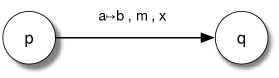
Figure 1. The transition function $\delta$

In this section we shall use a pictorial representation of QTMs, via a graph for the transition function $\delta$. When $\delta(q,a)(p,b,d)=x$ with $x\neq 0$ we draw the labelled arc as in Figure 1.

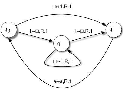
Figure 2. Reversible TM a là Bernstein and Vazirani

Example 41 (classical reversible TM with quantum behaviour).

Let $M$ be the reversible TM represented in Figure 2, where $a\in\{\Box,1\}$. $M$ is a B&V-QTM indeed.

If we feed $M$ with a non classical input, e.g. $\left|\mathsf{\psi}\right\rangle=\frac{1}{\sqrt{2}}\left|\mathsf{\underline{1}}\right\rangle+\frac{1}{\sqrt{2}}\left|\mathsf{\underline{3}}\right\rangle$, then $M$ fails to give an answer according to B&V’s framework, since B&V-QTMs always presuppose a classical input.

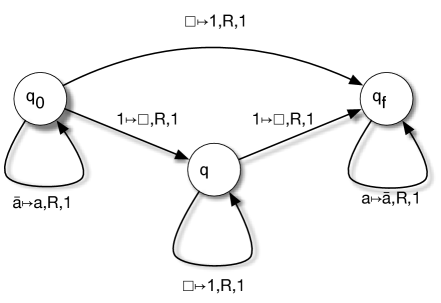
Figure 3. Reversible TM

If we transform $M$ in our formalism (see Theorem 13), we obtain the QTM in Figure 3. From the definition of computed output, we have that $M_{\frac{1}{\sqrt{2}}\left|\mathsf{\underline{1}}\right\rangle+\frac{1}{\sqrt{2}}\left|\mathsf{\underline{3}}\right\rangle}\to\{\frac{1}{2}:2\}$; namely, with probability $\frac{1}{2}$ the QTM halts with output $2$; while with probability $\frac{1}{2}$ it diverges.

Example 42 (A PD obtained as a limit).

The following example shows a machine which produces a PD only as an infinite limit. Let us consider the QTM in Figure 4, where $\Sigma=\{\$,1,\Box\}$, $a\in\{1,\Box\}$, $p$ is a target state, and $s$ is a source state. A simple calculation show that $M_{\left|\mathsf{\underline{n}}\right\rangle}\to\{1:n+1\}$; namely, the machine $M$ on input $n$ produces with probability $1$ the successor $n+1$. We can see also that the PD $\{1:n+1\}$ is obtained only as a limit. Of course we must not wait an infinite time to readback the result! A correct way to interpret this fact, is that for each $n\in\mathbb{N}$, each $\epsilon\in(0,\frac{1}{2}]$ there exist a natural number $j$ s.t. $\mathbf{P}_{U^{j}\left|\mathsf{\underline{n}}\right\rangle}(n+1)>1-\epsilon$.

Figure 4. Identity

6. Conclusions and further work

We find surprising that in the thirty years since [10] a theory of quantum computable functions did not develop, and that the main interest remained in QTMs as computing devices for classical problems/functions. This in sharp contrast with the original (Feynman’s and Deutsch’s) aim to have a better computing simulation of the physical world.

As always in these foundational studies, we had to go back to the basics, and look for a notion of QTM general enough to encompass previous approaches (for instance, simulation of B&V-QTMs, Theorem 13), and still sufficiently constrained to allow for a neat mathematical framework (for instance, monotonicity of quantum computations, Theorem 19, a consequence of the particular way final states are treated in order to defuse quantum interference once such states are entered). While several details of the proposed approach may well change during further study, we are particularly happy to have a recursive enumerable class of QTMs. This may allow a fresh look to the problem of a quantum universal machine, and, therefore, to obtain some of the “standard” theorems of classical computability theory (s-m-n, normal form, recursion, etc.). These themes, as well those related to the various degrees of partiality of quantum computable functions (see the brief discussion after Proposition 24) will be the subject of forthcoming papers.

Appendix A Hilbert spaces with denumerable basis

Definition 43 (Hilbert space of configurations).

Given a denumerable set $\mathcal{B}$, with $\ell^{2}(\mathcal{B})$ we shall denote the infinite dimensional Hilbert space defined as follow.

The set of vectors in $\ell^{2}(\mathcal{B})$ is the set

$$\left\{\phi\;|\;\phi:\mathcal{B}\rightarrow\mathbb{C},\sum_{C\in\mathcal{B}}|\phi(C)|^{2}<\infty\right\}$$

and equipped with:

1. An inner sum $+:\ell^{2}(\mathcal{B})\times\ell^{2}(\mathcal{B})\to\ell^{2}(\mathcal{B})$
   defined by $(\phi+\psi)(C)=\phi(C)+\psi(C)$;

2. A multiplication by a scalar $\cdot:\mathbb{C}\times\ell^{2}(\mathcal{B})\to\ell^{2}(\mathcal{B})$
   defined by $(a\cdot\phi)(C)=a\cdot(\phi(C))$;

3. An inner product $\left\langle\cdot,\cdot\right\rangle:\ell^{2}(\mathcal{B})\times\ell^{2}(\mathcal{B})\to\mathbb{C}$
   defined by $\left\langle\phi,\psi\right\rangle=\sum_{C\in\mathcal{B}}\phi(C)^{*}\psi(C)$;

4. The Euclidian norm is defined as $\left\|\phi\right\|=\left\langle\phi,\phi\right\rangle$.

The Hilbert space $\ell^{2}=\ell^{2}(\mathbb{N})$ is the standard Hilbert space of denumerable dimension—all the Hilbert spaces with denumerable dimension are isomorphic to it. $\ell^{2}_{1}$ is the set of the vectors of $\ell^{2}$ with unitary norm.

Definition 44 (computational basis).

The set of functions

$$\mathsf{CB}(\mathcal{B})=\{\left|\mathsf{C}\right\rangle:C\in\mathcal{B},\ \left|\mathsf{C}\right\rangle:\mathcal{B}\to\mathbb{C}\}$$

such that for each $C$

$$\left|\mathsf{C}\right\rangle(D)=\left\{\begin{array}[]{ll}1&\mbox{if}\;C=D\\ 0&\mbox{if}\;C\neq D\end{array}\right.$$

is called computational basis of $\ell^{2}(\mathcal{B})$.

We can prove that [17]:

Theorem 45.

The set $\mathsf{CB}(\mathcal{B})$ is an Hilbert basis of $\ell^{2}(\mathcal{B})$.

Let us note that the inner product space $\mathsf{span}(\mathsf{CB}(\mathcal{B}))$ defined by:

$$\mathsf{span}(\mathsf{CB}(\mathcal{B}))=\left\{\sum_{i=1}^{n}c_{i}S_{i}\ |\ c_{i}\in\mathbb{C},S_{i}\in\mathsf{CB}(\mathcal{B}),n\in\mathbb{N}\right\}.$$

is a proper inner product subspace of $\ell^{2}(\mathcal{B})$, but it is not an Hilbert Space (this means that $\mathsf{CB}(\mathcal{B})$ is not an Hamel basis of $\ell^{2}(\mathcal{B})$).

The completion of $\mathsf{span}(\mathsf{CB}(\mathcal{B}))$ is a space isomorphic to $\ell^{2}(\mathcal{B})$.

By means of a standard result in functional analysis we have:

Theorem 46.

1. $\mathsf{span}(\mathsf{CB}(\mathcal{B}))$ is a dense subspace of $\ell^{2}(\mathcal{B})$;

2. $\ell^{2}(\mathcal{B})$ is the (unique! up to isomorphism) completion of $\mathsf{span}(\mathsf{CB}(\mathcal{B}))$.

Definition 47.

Let $\mathcal{V}$ be a complex inner product space, a linear application $U:\mathcal{V}\to\mathcal{V}$ is called an isometry if $\left\langle Ux,Uy\right\rangle=\left\langle x,y\right\rangle$, for each $x,y\in\mathcal{V}$; moreover if $U$ is also surjective, then it is called unitary.

Since an isometry is injective, a unitary operator is invertible, and moreover, its inverse is also unitary.

Definition 48.

Let $\mathcal{V}$ be a complex inner product vectorial space, a linear application $L:\mathcal{V}\to\mathcal{V}$ is called bounded if $\exists c>0\;\forall x\;|Lx|\leq c||x||$.

Theorem 49.

Let $\mathcal{V}$ be a complex inner product vectorial space, for each bounded application $U:\mathcal{V}\to\mathcal{V}$ there is one and only one bounded application $U^{*}:\mathcal{V}\to\mathcal{V}$ s.t. $\left\langle x,Uy\right\rangle=\left\langle U^{*}x,y\right\rangle$. We say that $U^{*}$ is the adjoint of $U$.

It is easy to show that if $U$ is a bounded application, then $U$ is unitary iff $U$ is invertible and $U^{*}=U^{-1}$.

Theorem 50.

Each unitary operator $U$ in $\mathsf{span}(\mathsf{CB}(\mathcal{B}))$ has an unique extension in $\ell^{2}(\mathcal{B})$ [3].

A.1. Dirac notation

We conclude this brief digest on Hilbert spaces, by a synopsis of the so-called Dirac notation, extensively used in the paper.

mathematical notion	Dirac notation
inner product $\left\langle\phi,\psi\right\rangle$	$\left\langle\mathsf{\phi}\mid\mathsf{\psi}\right\rangle$
vector $\phi$	$\left|\mathsf{\phi}\right\rangle$
dual of vector $\phi$	$\left\langle\mathsf{\phi}\right|$
i.e., the linear application $d_{\phi}$
defined as $d_{\phi}(\psi)=\left\langle\phi,\psi\right\rangle$	note that $\left\langle\mathsf{\phi}\mid\mathsf{\psi}\right\rangle=\left\langle\mathsf{\phi}\right|(\left|\mathsf{\psi}\right\rangle)$

Let $L$ be a linear application, with $\left\langle\mathsf{\phi}\right|L\left|\mathsf{\psi}\right\rangle$ we denote $\left\langle\mathsf{\phi}\mid\mathsf{L\psi}\right\rangle$.

Appendix B Proof of Theorem 7

In this section we shall give the proof of Theorem 7 in full details. Following Bernstein and Vazirani [3] and Nishimura and Ozawa [16], we shall prove a stronger result indeed, that the local unitary conditions are not only sufficient to obtain a unitary time evolution, but also necessary (Theorem 60).

B.1. Pre-QTM

A pre-QTM is a tuple $M=\langle\Sigma,\mathcal{Q},\mathcal{Q}_{s},\mathcal{Q}_{t},\delta,q_{i},q_{f}\rangle$ for which all the requirements demanded for a QTM (Definition 1) but the local unitary conditions hold. In other words, while $\delta_{s}$ and $\delta_{t}$ are defined and constrained as for QTM’s, we do not have any condition on $\delta_{0}$. Ground and quantum configurations, step function and time evolution operator of pre-QTM’s are defined as for QTM’s. In the following, $M$ will denote a pre-QTM.

B.2. Basic results

Let us start with some basic results which hold in any Hilbert space. As usual, if $U$ is an operator, $U^{*}$ denotes its adjoint.

Lemma 51.

Let $U:\ell^{2}(\mathfrak{C}_{M})\to\ell^{2}(\mathfrak{C}_{M})$.

1. $U$ is an isometry iff it is left-invertible and its adjoint is its left-inverse, that is, $U^{*}U=1$.

2. If $U$ is an isometry, then $P=UU^{*}$ is an orthonormal projection and

   1. $\left\|P\left|\mathsf{\phi}\right\rangle\right\|\leq\left\|\left|\mathsf{\phi}\right\rangle\right\|$, for every $\phi$;

   2. $\left\|P\left|\mathsf{\phi}\right\rangle\right\|=\left\|\left|\mathsf{\phi}\right\rangle\right\|$ iff $P\left|\mathsf{\phi}\right\rangle=\left|\mathsf{\phi}\right\rangle$;

   3. $P=1$ iff $\left\|P\left|\mathsf{C}\right\rangle\right\|=\left\langle\mathsf{C}\right|P\left|\mathsf{C}\right\rangle=1$, for every $C\in\mathfrak{C}_{M}$.

Proof.

1. $\langle U\left|\mathsf{\phi}\right\rangle,U\left|\mathsf{\psi}\right\rangle\rangle=\langle U^{*}U\left|\mathsf{\phi}\right\rangle,\left|\mathsf{\psi}\right\rangle\rangle=\left\langle\mathsf{\phi}\mid\mathsf{\psi}\right\rangle$ iff $U^{*}U=1^{*}=1$.

2. $P$ is a projection when $PP=P$ and, moreover, it is orthonormal when it is self-adjoint, that is $P^{*}=P$. Equivalently, $P$ is a projection iff, for every $\phi$, we have $\left|\mathsf{\phi}\right\rangle=\left|\mathsf{\phi_{1}}\right\rangle+\left|\mathsf{\phi_{0}}\right\rangle$ for some (unique) $\phi_{1}$ and $\phi_{0}$ s.t. $P\left|\mathsf{\phi_{1}}\right\rangle=\phi_{1}$ and $P\left|\mathsf{\phi_{0}}\right\rangle=0$; it is orthonormal when $\left\langle\mathsf{\phi_{1}}\mid\mathsf{\phi_{0}}\right\rangle=0$ indeed.

   $P=UU^{*}$ is clearly self-adjoint. Moreover, $PP=UU^{*}UU^{*}=UU^{*}=P$, since $U$ is an isometry and then $U^{*}U=1$. Thus, $P$ is an orthonormal projection.

   Let $\left|\mathsf{\phi}\right\rangle=\left|\mathsf{\phi_{1}}\right\rangle+\left|\mathsf{\phi_{0}}\right\rangle$ be an orthonormal decomposition as above. $\left\|\left|\mathsf{\phi}\right\rangle\right\|=\left\|\left|\mathsf{\phi_{1}}\right\rangle\right\|+2\Re\left\langle\mathsf{\phi_{1}}\mid\mathsf{\phi_{0}}\right\rangle+\left\|\left|\mathsf{\phi_{0}}\right\rangle\right\|=\left\|P\left|\mathsf{\phi_{1}}\right\rangle\right\|+\left\|\left|\mathsf{\phi_{0}}\right\rangle\right\|=\left\|P\left|\mathsf{\phi}\right\rangle\right\|+\left\|\left|\mathsf{\phi_{0}}\right\rangle\right\|$.

   1. $\left\|P\left|\mathsf{\phi}\right\rangle\right\|\leq\left\|P\left|\mathsf{\phi}\right\rangle\right\|+\left\|\left|\mathsf{\phi_{0}}\right\rangle\right\|=\left\|\left|\mathsf{\phi}\right\rangle\right\|$

   2. $\left\|P\left|\mathsf{\phi}\right\rangle\right\|=\left\|\left|\mathsf{\phi}\right\rangle\right\|$ iff $\left\|\left|\mathsf{\phi_{0}}\right\rangle\right\|=0$, that is, iff $\left|\mathsf{\phi_{0}}\right\rangle=0$.

   3. By the previous item, $P\left|\mathsf{\phi}\right\rangle=\left|\mathsf{\phi}\right\rangle$ for every $\phi$, iff $\left\|P\left|\mathsf{\phi}\right\rangle\right\|=\left\|\left|\mathsf{\phi}\right\rangle\right\|$ for every $\phi$, that is, iff $\left\|P\left|\mathsf{C}\right\rangle\right\|=\left\|\left|\mathsf{C}\right\rangle\right\|=1$ for every $C\in\mathfrak{C}_{M}$, that is, iff $\left\|P\left|\mathsf{C}\right\rangle\right\|=\langle P\left|\mathsf{C}\right\rangle,P\left|\mathsf{C}\right\rangle\rangle=\left\langle\mathsf{C}\right|P\left|\mathsf{C}\right\rangle=1$, for every $C\in\mathfrak{C}_{M}$.

∎

B.3. Reverse transitions

The reverse step function of $M$ is defined by

$$\overline{\gamma}_{\Sigma,\mathcal{Q}}(\langle\alpha v_{R},p,wv_{L}\beta\rangle,q,u,d)\simeq\begin{cases}\langle\alpha v_{R},q,u\beta\rangle&\qquad\mbox{when $d=L$}\\ \langle\alpha,q,uwv_{L}\beta\rangle&\qquad\mbox{when $d=R$}\end{cases}$$

Let us say that an $R$ or $L$ step of $\overline{\gamma}$ is an $R$-reverse or $L$-reverse step. We see that an $R/L$-reverse step of $\overline{\gamma}$ revert an $R/L$ step of the step function $\gamma$. While in $\gamma$ both the $L$-step and the $R$-step replace the same symbol, the current symbol of the configuration, in $\overline{\gamma}$ the symbols replaced by the $R$-reverse step and by the $L$-reverse step are in different positions. We have then a current $L$-reverse symbol $v_{L}$ and a current $R$-reverse symbol $v_{R}$.

Lemma 52.

Let $C\simeq\langle\alpha_{1}w_{1},q,u\beta_{1}\rangle$ and $D\simeq\langle\alpha_{2}v_{R},p,w_{2}v_{L}\beta_{2}\rangle$.

$$\overline{\gamma}(D,q,u,d)=C\qquad\mbox{iff}\qquad\gamma(C,p,v_{d},d)=D$$

Proof.

When $d=R$, we have $C\simeq\langle\alpha_{2},q,uw_{2}v_{L}\beta_{2}\rangle\simeq\overline{\gamma}(D,q,u,R)$ iff $\alpha_{1}w_{1}\simeq_{l}\alpha_{2}$ and $w_{2}v_{L}\beta_{2}\simeq_{r}\beta_{1}$ iff $\gamma(C,p,v_{R},R)\simeq\langle\alpha_{1}w_{1}v_{R},q,\beta_{1}\rangle\simeq D$. When $d=L$, we have $C\simeq\langle\alpha_{2}v_{R}w_{2},q,u\beta_{2}\rangle\simeq\overline{\gamma}(D,q,u,L)$ iff $\alpha_{1}\simeq_{l}\alpha_{2}v_{R}$ and $w_{1}=w_{2}$ and $\beta_{2}\simeq_{r}\beta_{1}$ iff $\gamma(C,p,v_{L},L)\simeq\langle\alpha_{1},q,w_{1}v_{L}\beta_{1}\rangle\simeq D$. ∎

Lemma 53.

Let $C[q,u]$ be the configuration obtained by substituting the state $q$ and the symbol $u$ for the current state and the current symbol of the configuration $C$, and let $C_{p,v,d_{1}}^{q,u,d_{2}}=\overline{\gamma}(\gamma(C,p,v,d_{1}),q,u,d_{2})$.

1. If $d=d_{1}=d_{2}$, then $C[q,u]=C^{p,v,d}_{q,u,d}$, for every $(p,v)\in\mathcal{Q}\times\widehat{\Sigma}$.

2. When $d_{1}\neq d_{2}$, there is $C_{d_{1}d_{2}}[q,u,v]$, which does not depend on $p$, s.t. $C_{d_{1}d_{2}}[q,u,v]=C_{p,v,d_{1}}^{q,u,d_{2}}$, for every $p\in\mathcal{Q}$.

Moreover, let $(q^{\prime},u^{\prime},v^{\prime}),(q^{\prime\prime},u^{\prime\prime},v^{\prime\prime})\in\mathcal{Q}\times\widehat{\Sigma}\times\widehat{\Sigma}$ and $d_{1},d_{2},d_{1}^{\prime},d_{2}^{\prime}\in\mathbb{D}_{x}$ with $d_{1}\neq d_{2}$ and $d_{1}^{\prime}\neq d_{2}^{\prime}$. If the tape of the configuration $C$ contains at least a non-empty cell in addition to the current one (that is, $C\neq\langle\lambda,q,u\lambda\rangle$), then

1. $C[q^{\prime},u^{\prime}]=C[q^{\prime\prime},u^{\prime\prime}]$ iff $(q^{\prime},u^{\prime})=(q^{\prime\prime},u^{\prime\prime})$;

2. $C[q^{\prime},u^{\prime}]\neq C_{d_{1}d_{2}}[q^{\prime\prime},u^{\prime\prime},v^{\prime\prime}]$;

3. $C_{d_{1}d_{2}}[q^{\prime},u^{\prime},v^{\prime}]=C_{d_{1}^{\prime}d_{2}^{\prime}}[q^{\prime\prime},u^{\prime\prime},v^{\prime\prime}]$ iff $(d_{1},d_{2})=(d_{1}^{\prime},d_{2}^{\prime})$ and $(q^{\prime},u^{\prime},v^{\prime})=(q^{\prime\prime},u^{\prime\prime},v^{\prime\prime})$

Proof.

Let $C\simeq\langle\alpha z_{l}w_{l},q,uw_{r}z_{r}\beta\rangle$. By computing $C_{p,v,d_{1}}^{q,u,d_{2}}$, we see that (1) and (2) hold with

$$C[q^{\prime},u^{\prime}] \simeq\langle\alpha z_{l}w_{l},q^{\prime},u^{\prime}w_{r}z_{r}\beta\rangle$$

$$C_{LR}[q^{\prime},u^{\prime},v] \simeq\langle\alpha,q^{\prime},u^{\prime}w_{l}vw_{r}z_{r}\beta\rangle$$

$$C_{RL}[q^{\prime},u^{\prime},v] \simeq\langle\alpha z_{l}w_{l}vw_{r},q^{\prime},u^{\prime}\beta\rangle$$

From which, we can prove the following items.

1. Immediate.

2. Let $C[q^{\prime},u^{\prime}]\simeq C_{LR}[q^{\prime\prime},u^{\prime\prime},v^{\prime\prime}]$. Then, $\alpha z_{l}w_{l}\simeq_{l}\alpha$ and $q^{\prime}=q^{\prime\prime}$ and $u^{\prime}w_{r}z_{r}\beta\simeq_{R}u^{\prime\prime}w_{l}v^{\prime\prime}w_{r}z_{r}\beta$. Which is possible only if $\alpha\simeq\beta\simeq\lambda$ and $z_{l}=z_{r}=w_{l}=w_{r}=v^{\prime\prime}=\Box$ and $u^{\prime}=u^{\prime\prime}$. But this is the case only if $C=\langle\lambda,q,u\lambda\rangle$. And analogously for $C[q^{\prime},u^{\prime}]\simeq C_{RL}[q^{\prime\prime},u^{\prime\prime},v^{\prime\prime}]$, it may hold only if $C=\langle\lambda,q,u\lambda\rangle$.

3. The case $(d_{1},d_{2})=(d_{1}^{\prime},d_{2}^{\prime})$ is immediate. Thus, let us assume $C_{LR}[q^{\prime},u^{\prime},v^{\prime}]\simeq C_{RL}[q^{\prime\prime},u^{\prime\prime},v^{\prime\prime}]$. We see that this is possible only if $\alpha\simeq_{l}\alpha z_{l}w_{l}v^{\prime\prime}w_{r}$ and $q^{\prime}=q^{\prime\prime}$ and $u^{\prime}w_{l}v^{\prime}w_{r}z_{r}\beta\simeq_{r}u^{\prime\prime}\beta$. Which holds only if $\alpha\simeq\beta\simeq\lambda$ and $z_{l}=z_{r}=w_{l}=w_{r}=v^{\prime}=v^{\prime\prime}=\Box$ and $u^{\prime}=u^{\prime\prime}$. That implies $C=\langle\lambda,q,u\lambda\rangle$.

∎

Lemma 54.

Let $\overline{C}_{p,v,d_{2}}^{q,u,d_{1}}=\gamma(\overline{\gamma}(C,q,u,d_{1}),p,v,d_{2})$.

1. There is a triple $(q,w_{L},w_{R})\in\mathcal{Q}\times\widehat{\Sigma}\times\widehat{\Sigma}$, s.t., for any $(q^{\prime},u^{\prime})\in Q\times\widehat{\Sigma}$ and $d=\mathbb{D}_{x}$, we have $C=\overline{C}_{p,v,d}^{q^{\prime},u^{\prime},d}$ iff $(p,v)=(q,w_{d})$.

2. For $d_{1}\neq d_{2}\in\mathbb{D}_{x}$, $C=\overline{C}_{p,v,d_{1}}^{q^{\prime},u^{\prime},d_{2}}$, iff $C=\langle\lambda,q,\lambda\rangle$ and $u^{\prime}=v=\lambda$ and $p=q$.

Proof.

1. Let us define $\overline{C}_{R}[q^{\prime},u^{\prime}]=\langle\alpha z_{1}u^{\prime},q^{\prime},uw_{L}z_{2}\beta\rangle$ (the configuration obtained by replacing $q^{\prime}$ and $u^{\prime}$ for the current state $q$ and the reverse right symbol $w_{R}$ of $C$) and $\overline{C}_{L}[q^{\prime},u^{\prime}]=\langle\alpha z_{1}w_{R},q^{\prime},uu^{\prime}z_{2}\beta\rangle$ (the configuration obtained by replacing $q^{\prime}$ and $u^{\prime}$ for the current state $q$ and the reverse right symbol $w_{R}$ of $C$), it is readily seen that $C_{q^{\prime},u^{\prime},d}^{p,v,d}=C_{d}[p,v]$ and, as a consequence, $C=C_{d}[p,v]$ iff $(p,v)=(q,u)$.

2. By direct computation, we see that $\overline{C}_{p,v,L}^{q^{\prime},u^{\prime},R}=\langle\alpha z_{l}w_{R}uu^{\prime}v,p,\beta\rangle$ and $\overline{C}_{p,v,R}^{q^{\prime},u^{\prime},L}=\langle\alpha,p,vu^{\prime}uw_{L}z_{R}\beta\rangle$. From which, we see that $C=\overline{C}_{p,v,L}^{q^{\prime},u^{\prime},R}$ iff $\alpha=\beta=\lambda$ and $z_{L}=z_{R}=w_{L}=w_{R}=u=u^{\prime}=v=\Box$ and $C=\overline{C}_{p,v,R}^{q^{\prime},u^{\prime},L}$ iff $z_{L}=z_{R}=w_{L}=w_{R}=u=u^{\prime}=v=\Box$.

∎

B.4. The adjoint of $U_{M}$

We can now compute the adjoint of the operator $U_{M}$. For this, we have already given the reverse transition $\overline{\gamma}$, but we also need to reverse the quantum transition function $\delta$. For $x\in\{0,s,t\}$, let us take

$$\overline{\delta}_{x}:\mathcal{T}_{x}\to\ell^{2}(\mathcal{S}_{x}\times\mathbb{D}_{x})\qquad\mbox{s.t.}\qquad\overline{\delta}_{x}(p,v)(q,u,d)=\delta_{x}(q,u)(p,v,d)^{*}$$

where $\mathbb{D}_{0}=\mathbb{D}$ and $\mathbb{D}_{s}=\mathbb{D}_{t}=\{R\}$. Then, let us define

$$\overline{\mathfrak{C}}^{x}_{M}=\{\langle\alpha v,p,\beta\rangle\in\mathfrak{C}_{M}\mid(p,v)\in\mathcal{T}_{x}\}$$

It is readily seen that $\overline{\mathfrak{C}}^{0}_{M}$, $\overline{\mathfrak{C}}^{s}_{M}$ and $\overline{\mathfrak{C}}^{t}_{M}$ are a partition of $\mathfrak{C}$, since they are pairwise disjoint and $\mathfrak{C}=\overline{\mathfrak{C}}^{0}_{M}\cup\overline{\mathfrak{C}}^{s}_{M}\cup\overline{\mathfrak{C}}^{t}_{M}$. Moreover, given

$$C\simeq\langle\alpha v_{R},p,wv_{L}\beta\rangle\in\overline{\mathfrak{C}}^{x}_{M}$$

we have that, $(p,v_{R})\in\mathcal{T}_{x}$ by definition, and when $x=0$, that $(p,v_{L})\in\mathcal{T}_{0}$ also (since by the definition of ground configuration, $p\in\mathcal{Q}_{0}\cup\mathcal{Q}_{t}$ implies that $wv_{L}\beta\in\Sigma^{*}$). Thus, we can finally define

$$W^{*}_{M}\left|\mathsf{C}\right\rangle =\quad\sum_{(q,u,d)\in\mathcal{S}_{x}\times\mathbb{D}_{x}}\overline{\delta}_{x}(p,v_{d})(q,u,d)\,\left|\mathsf{C_{q,u,d}}\right\rangle$$

$$=\quad\sum_{(q,u,d)\in\mathcal{S}_{x}\times\mathbb{D}_{x}}\delta_{x}(q,u)(p,v_{d},d)^{*}\,\left|\mathsf{C_{q,u,d}}\right\rangle$$

where $C_{q,u,d}=\overline{\gamma}_{\Sigma,\mathcal{Q}}(C,q,u,d)$.

We remark that, w.r.t. the definition of $W_{M}$, in the range of the sum in $W_{M}^{*}$, we have $\mathcal{S}_{x}\times\mathbb{D}_{x}$ in the place of $\mathcal{T}_{x}\times\mathbb{D}$. In the case $x=0$, there is no difference, since $\mathbb{D}_{x}=\mathbb{D}$ and then we consider both the reverse deplacements; in the case $x=s,t$ instead, $\mathbb{D}_{x}=\{R\}$ and then we consider the $R$ deplacement only. Technically, this is necessary as in these cases $(p,v_{L})\not\in\mathcal{T}_{x}$, and then $\delta(q,u)(p,v_{L},d)$ would not be defined. Indeed , for $x=s,t$, any configuration in $\overline{\mathfrak{C}}^{x}_{M}$ can be entereded from an $R$ deplacement only; then, in this case, to reverse the quantum transition functions it suffices to consider $R$ reverse deplacements only. On the other hand, even in the definition of $W_{M}$, we might have restricted the sum to the $R$ deplacement only, in the case $x=s,t$. Indeed,

$$W_{M}(\left|\mathsf{C}\right\rangle)=\sum_{(p,v,d)\in\mathcal{T}_{x}\times\mathbb{D}_{x}}\delta_{x}(q,u)(p,v,d)\,\left|\mathsf{C_{p,v,d}}\right\rangle$$

for $C=\langle\alpha,q,u\beta\rangle\in\mathfrak{C}^{x}_{M}$, and $x=0,s,t$.

Lemma 55.

$W_{M}^{*}\left|\mathsf{C}\right\rangle\in\mathsf{span}(\mathsf{CB}(\mathfrak{C}))$, for every $C\in\mathfrak{C}_{M}$. Then, $W_{M}^{*}$ defines an automorphism

$$W_{M}^{*}:\mathsf{span}(\mathsf{CB}(\mathfrak{C}))\to\mathsf{span}(\mathsf{CB}(\mathfrak{C}))$$

of the linear space $\mathsf{span}(\mathsf{CB}(\mathfrak{C}))$.

Proof.

By case analysis, as in the proof of Proposition 5. ∎

We can also see that $W_{M}^{*}$ maps every $\overline{\mathfrak{C}}^{x}_{M}$ into $\mathfrak{C}^{x}_{M}$, which is indeed the converse of the fact that $W_{M}$ maps $\mathfrak{C}^{x}_{M}$ into $\overline{\mathfrak{C}}^{x}_{M}$.

Lemma 56.

1. $W_{M}({\mathsf{span}(\mathsf{CB}(\mathfrak{C}^{x}_{M}))})\subseteq\mathsf{span}(\mathsf{CB}(\overline{\mathfrak{C}}^{x}_{M}))$

2. $W_{M}^{*}({\mathsf{span}(\mathsf{CB}(\overline{\mathfrak{C}}^{x}_{M}))})\subseteq\mathsf{span}(\mathsf{CB}(\mathfrak{C}^{x}_{M}))$.

Proof.

By case analysis. ∎

We can now prove that $W_{M}^{*}$ defines the adjoint of $U_{M}$.

Lemma 57.

The unique extension of $W_{M}^{*}$ to the Hilbert space $\ell^{2}(\mathfrak{C}_{M})$ is the adjoint $U_{M}^{*}$ of $U_{M}$.

Proof.

It suffices to prove that $\left\langle W_{M}^{*}\left|\mathsf{D}\right\rangle,\left|\mathsf{C}\right\rangle\right\rangle=\left\langle\mathsf{D}\right|W_{M}\left|\mathsf{C}\right\rangle$, for every $C,D\in\mathfrak{C}_{M}$. Let $C\in\mathfrak{C}^{x}$ and $D\in\overline{\mathfrak{C}}^{y}$, with $x,y\in\{0,s,t\}$. Since $\left\langle W_{M}^{*}\left|\mathsf{D}\right\rangle,\left|\mathsf{C}\right\rangle\right\rangle=\left\langle\mathsf{D}\right|W_{M}\left|\mathsf{C}\right\rangle=0$ if $x\neq y$ (by Lemma 56), we have to analyse the cases $x=y$ only.

Let $C\simeq\langle\alpha_{1}w_{1},q,u\beta_{1}\rangle\in\mathfrak{C}^{x}$, $D\simeq\langle\alpha_{2}v_{R},p,w_{2}v_{L}\beta_{2}\rangle\in\overline{\mathfrak{C}}^{x}$, $D_{q,u,d}=\overline{\gamma}(D,q,u,d)$, and $C_{p,v,d}=\gamma(C,p,v,d)$. Let us start with the case $x=0$.

$$\left\langle W^{*}_{M}\left|\mathsf{D}\right\rangle,\left|\mathsf{C}\right\rangle\right\rangle =\quad\sum_{(q^{\prime},u^{\prime},d)\in\mathcal{S}_{x}\times\mathbb{D}_{x}}\overline{\delta}_{x}(p,v_{d})(q^{\prime},u^{\prime},d)^{*}\,\left\langle\mathsf{D_{q^{\prime},u^{\prime},d}}\mid\mathsf{C}\right\rangle$$

$$=\quad\sum_{(q^{\prime},u^{\prime},d)\in\mathcal{S}_{x}\times\mathbb{D}_{x}}\delta_{x}(q^{\prime},u^{\prime})(p,v_{d},d)\,\left\langle\mathsf{D_{q^{\prime},u^{\prime},d}}\mid\mathsf{C}\right\rangle$$

$$=\quad\sum_{d\in\mathbb{D}_{x}}\delta_{x}(q,u)(p,v_{d},d)\,\left\langle\mathsf{D_{q,u,d}}\mid\mathsf{C}\right\rangle$$

$$=\quad\sum_{d\in\mathbb{D}_{x}}\delta_{x}(q,u)(p,v_{d},d)\,\left\langle\mathsf{D}\mid\mathsf{C_{p,v_{d},d}}\right\rangle$$

$$=\quad\sum_{(p^{\prime},v^{\prime},d)\in\mathcal{T}_{x}\times\mathbb{D}_{x}}\delta_{x}(q,u)(p^{\prime},v^{\prime},d)\,\left\langle\mathsf{D}\mid\mathsf{C_{p^{\prime},v^{\prime},d}}\right\rangle$$

$$=\quad\left\langle\mathsf{D}\right|W_{M}\left|\mathsf{C}\right\rangle$$

Where we have used the facts that $\left\langle\mathsf{D_{q^{\prime},u^{\prime},d}}\mid\mathsf{C}\right\rangle=0$ if $(q^{\prime},u^{\prime})\neq(q,u)$, that $\left\langle\mathsf{D}\mid\mathsf{C_{p^{\prime},v^{\prime},d}}\right\rangle=0$ if $(p^{\prime},v^{\prime})\neq(p,v_{d})$ (by inspection, we see that in these cases the above configurations differ for the current state or for the current symbol), and that $\left\langle\mathsf{D_{q,u,d}}\mid\mathsf{C}\right\rangle=\left\langle\mathsf{D}\mid\mathsf{C_{p,v_{d},d}}\right\rangle$, by Lemma 52. ∎

B.5. Unitarity of the time evolution operator

In the following, we shall complete the proof that the time evolution operator of a QTM is unitary. Firstly, we show that the time evolution operator $U_{M}$ of a pre-QTM $M$ is an isometry iff the local unitary conditions hold (Lemma 58), then we shall see that, in the particular case of pre-QTMs, $U_{M}$ is unitary when it is is an isometry (Lemma 59). Therefore, a pre-QTM is a QTM iff its time evolution operator is unitary.

Lemma 58.

$U_{M}^{*}U_{M}=1$ iff the local unitary conditions holds, that is, $U_{M}$ is an isometry iff $M$ is a QTM.

Proof.

It suffices to prove that, for $C\in\mathfrak{C}^{x}_{M}$, with $x\in\{0,s,t\}$,

$$W_{M}^{*}W_{M}\left|\mathsf{C}\right\rangle\quad=\sum_{(p,v,d)\in\mathcal{T}_{x}\times\mathbb{D}}\delta_{x}(q,u)(p,v,d)\,W_{M}^{*}\left|\mathsf{C_{p,v,d}}\right\rangle\quad=\quad 1$$

iff the local unitary conditions hold.

Let us assume

$$C\simeq\langle\alpha v_{R}w,q,uzv_{L}\beta\rangle\in\mathfrak{C}^{x}$$

$$C_{p,v,d}=\gamma(C,p,v,d)\qquad\qquad C_{p,v,d}^{q^{\prime},u^{\prime},d^{\prime}}=\overline{\gamma}(\gamma(C,p,v,d),q^{\prime},u^{\prime},d^{\prime})$$

we have

$$C_{p,v,L}\simeq\langle\alpha v_{R},q,wvzv_{L}\beta\rangle\qquad\qquad C_{p,v,R}\simeq\langle\alpha v_{R}wv,q,zv_{L}\beta\rangle$$

The cases $x=s$ and $x=t$ are immediate. For instance, if $x=t$, we have $(q,u)\in\mathcal{Q}_{t}\times\Sigma$, and $\delta_{t}(q,u)(p,v,d)=1$, when $(p,v,d)=(q,\overline{u},R)$, while $\delta_{t}(q,u)(p,v,d)=0$, otherwise. Thus

$$W_{M}^{*}W_{M}\left|\mathsf{C}\right\rangle\quad=\quad W_{M}^{*}\left|\mathsf{C_{q,\overline{u},R}}\right\rangle\quad=\sum_{(q^{\prime},u^{\prime})\in\mathcal{S}_{t}}\delta_{t}(q^{\prime},u^{\prime})(q,\overline{u},R)^{*}\left|\mathsf{C^{q^{\prime},u^{\prime},R}_{q,\overline{u},R}}\right\rangle$$

but $\delta_{t}(q^{\prime},u^{\prime})(p,\overline{u},R)=1$, $(p,u)=(q^{\prime},u^{\prime})$, and $\delta_{t}(q^{\prime},u^{\prime})(p,\overline{u},r)=0$, otherwise; thus

$$W_{M}^{*}W_{M}\left|\mathsf{C}\right\rangle\quad\quad=\quad\left|\mathsf{C^{q,u,R}_{q,\overline{u},R}}\right\rangle\quad=\quad\left|\mathsf{C}\right\rangle$$

(by Lemma 53) and analogously for the case $x=s$. Therefore, for $x\in\{s,t\}$, since the equivalence holds for every pre-QTM.

Let us now analyse the case $x=0$. By definition,

$$W_{M}^{*}\left|\mathsf{C_{p,v,d}}\right\rangle=\sum_{(q^{\prime},u^{\prime},d^{\prime})}=\delta_{0}(q^{\prime},u^{\prime})(p,v^{\prime}_{d^{\prime}},d^{\prime})^{*}\,\left|\mathsf{C^{q^{\prime},u^{\prime},d^{\prime}}_{p,v,d}}\right\rangle$$

for some $v^{\prime}_{d^{\prime}}$ that depend on $C_{p,v,d}$. By reorganizing the sums according to the cases $d^{\prime}=d$ and $d^{\prime}\neq d$, we get

$$W_{M}^{*}W_{M}\left|\mathsf{C}\right\rangle\quad=\sum_{(p,v,d)\in\mathcal{T}_{x}\times\mathbb{D}}\delta_{0}(q,u)(p,v,d)\,W_{M}^{*}\left|\mathsf{C_{p,v,d}}\right\rangle\\ \begin{aligned} \qquad&=\sum_{(p,v,d)\in\mathcal{T}_{x}\times\mathbb{D}}\sum_{(q^{\prime},u^{\prime})\in\mathcal{S}_{x}}\delta_{0}(q,u)(p,v,d)\,\delta_{0}(q^{\prime},u^{\prime})(p,v,d)^{*}\,\left|\mathsf{C^{q^{\prime},u^{\prime},d}_{p,v,d}}\right\rangle\\ &\quad+\sum_{(p,v)\in\mathcal{T}_{x}}\sum_{(q^{\prime},u^{\prime})\in\mathcal{S}_{x}}\delta_{0}(q,u)(p,v,L)\,\delta_{0}(q^{\prime},u^{\prime})(p,v_{R},R)^{*}\,\left|\mathsf{C^{q^{\prime},u^{\prime},R}_{p,v,L}}\right\rangle\\ &\quad+\sum_{(p,v)\in\mathcal{T}_{x}}\sum_{(q^{\prime},u^{\prime})\in\mathcal{S}_{x}}\delta_{0}(q,u)(p,v,R)\,\delta_{0}(q^{\prime},u^{\prime})(p,v_{L},L)^{*}\,\left|\mathsf{C^{q^{\prime},u^{\prime},L}_{p,v,R}}\right\rangle\\ \end{aligned}$$

By Lemma 53, this corresponds to

$$W_{M}^{*}W_{M}\left|\mathsf{C}\right\rangle\\ \begin{aligned} \quad&=\sum_{(p,v,d)\in\mathcal{T}_{0}\times\mathbb{D}}|\delta_{0}(q,u)(p,v,d)|^{2}\,\left|\mathsf{C}\right\rangle\\ &\ +\sum_{(q^{\prime},u^{\prime})\in\mathcal{S}_{0}\setminus\{(q,u)\}}\;\sum_{(p,v,d)\in\mathcal{T}_{0}\times\mathbb{D}}\delta_{0}(q,u)(p,v,d)\,\delta_{0}(q^{\prime},u^{\prime})(p,v,d)^{*}\,\left|\mathsf{C[q^{\prime},u^{\prime}]}\right\rangle\\ &\ +\sum_{(q^{\prime},u^{\prime})\in\mathcal{S}_{0}}\;\sum_{v\in\Sigma}\;\sum_{p\in\mathcal{Q}_{0}\cup\mathcal{Q}_{t}}\delta_{0}(q,u)(p,v,R)\,\delta_{0}(q^{\prime},u^{\prime})(p,v_{L},L)^{*}\,\left|\mathsf{C_{RL}[q^{\prime},u^{\prime},v]}\right\rangle\\ &\ +\sum_{(q^{\prime},u^{\prime})\in\mathcal{S}_{0}}\;\sum_{v\in\Sigma}\;\sum_{p\in\mathcal{Q}_{0}\cup\mathcal{Q}_{t}}\delta_{0}(q,u)(p,v,L)\delta_{0}(q^{\prime},u^{\prime})(p,v_{R},R)^{*}\,\left|\mathsf{C_{LR}[q^{\prime},u^{\prime},v]}\right\rangle\end{aligned}$$

where, $C$, $C[q^{\prime}u^{\prime}]$, $C_{LR^{\prime}}[q^{\prime},u^{\prime},v]$, and $C_{RL}[q^{\prime},u^{\prime},v]$ are never equal, does not depend on $(p,v)$, and $C$, $C[q^{\prime}u^{\prime}]$ are independent from $d$ also.

From which we may conclude that, $W_{M}^{*}W_{M}\left|\mathsf{C}\right\rangle=\left|\mathsf{C}\right\rangle$ for every $C\in\mathfrak{C}^{0}$, iff for every $q,q^{\prime}\in\mathcal{Q}_{0}\cup\mathcal{Q}_{s}$ and $v,u,u^{\prime}v_{L},v_{R}\in\Sigma$

$$1 =\sum_{(p,v,d)\in\mathcal{T}_{0}\times\mathbb{D}}|\delta_{0}(q,u)(p,v,d)|^{2}$$

$$0 =\sum_{(p,v,d)\in\mathcal{T}_{0}\times\mathbb{D}}\delta_{0}(q,u)(p,v,d)\,\delta_{0}(q^{\prime},u^{\prime})(p,v,d)^{*}$$

$$0 =\sum_{p\in\mathcal{Q}_{0}\cup\mathcal{Q}_{t}}\delta_{0}(q,u)(p,v,R)\,\delta_{0}(q^{\prime},u^{\prime})(p,v_{L},L)^{*}$$

$$0 =\sum_{p\in\mathcal{Q}_{0}\cup\mathcal{Q}_{t}}\delta_{0}(q,u)(p,v,L)\delta_{0}(q^{\prime},u^{\prime})(p,v_{R},R)^{*}$$

that is, iff the local unitary conditions hold. ∎

Lemma 59.

If $U_{M}$ is an isometry, then $U_{M}U_{M}^{*}=1$. As a consequence, $U_{M}$ is unitary.

Proof.

Since $U_{M}$ is an isometry, by Lemma 51 we know that $U_{M}U_{M}^{*}$ is an orthonormal projection and $U_{M}U_{M}^{*}=1$ iff $\left\langle\mathsf{C}\right|U_{M}U_{M}^{*}\left|\mathsf{C}\right\rangle=\left\langle\mathsf{C}\right|W_{M}W_{M}^{*}\left|\mathsf{C}\right\rangle=1$ for every $C\in\mathfrak{C}_{M}$.

Let us assume that

$$C\simeq\langle\alpha v_{R},p,wv_{L}\beta\rangle\in\overline{\mathfrak{C}}^{x}$$

$$\overline{C}_{q,u,d}=\gamma(C,q,u,d)\qquad\qquad\overline{C}_{p^{\prime},v^{\prime},d^{\prime}}^{q,u,d}=\gamma(\overline{\gamma}(C,q,u,d),p^{\prime},v^{\prime},d^{\prime})$$

we have

$$\overline{C}_{q,u,L}\simeq\langle\alpha v_{R}w,q,u\beta\rangle\qquad\qquad\overline{C}_{q,u,R}\simeq\langle\alpha,q,uwv_{L}\beta\rangle$$

$$\left\langle\mathsf{C}\right|W_{M}W_{M}^{*}\left|\mathsf{C}\right\rangle\\ \begin{aligned} \quad&=\sum_{(q,u,d)\in\mathcal{S}_{x}\times\mathbb{D}_{x}}\delta_{x}(q,u)(p,v_{d},d)^{*}\,\left\langle\mathsf{C}\right|W_{M}\left|\mathsf{\overline{C}_{q,u,d}}\right\rangle\\ \quad&=\sum_{\genfrac{}{}{0.0pt}{1}{(q,u,d)\in\mathcal{S}_{x}\times\mathbb{D}_{x}}{(p^{\prime},v^{\prime},d^{\prime})\in\mathcal{T}_{x}\times\mathbb{D}_{x}}}\delta_{x}(q,u)(p,v_{d},d)^{*}\delta_{x}(q,u)(p^{\prime},v^{\prime},d^{\prime})\,\left\langle\mathsf{C}\mid\mathsf{\overline{C}_{p^{\prime},v^{\prime},d^{\prime}}^{q,u,d}}\right\rangle\end{aligned}$$

By Lemma 54, we have that

1. when $d=d^{\prime}$

   $$\left\langle\mathsf{C}\mid\mathsf{\overline{C}_{p^{\prime},v^{\prime},d^{\prime}}^{q,u,d}}\right\rangle=\left\langle\mathsf{C}\mid\mathsf{\overline{C}_{p^{\prime},v^{\prime},d}^{q,u,d}}\right\rangle=\begin{cases}1&\qquad\mbox{if $(p^{\prime},v^{\prime})=(p,v_{d})$}\\ 0&\qquad\mbox{otherwise}\end{cases}$$

2. when $d\neq d^{\prime}$

   $$\left\langle\mathsf{C}\mid\mathsf{\overline{C}_{p^{\prime},v^{\prime},d^{\prime}}^{q,u,d}}\right\rangle=\begin{cases}1&\qquad\begin{minipage}[t]{142.26378pt} if $C=\langle\lambda,p,\lambda\rangle$ and $p=p^{\prime}$\\ and $v_{L}=v_{R}=v^{\prime}=u=\Box$ \end{minipage}\\ 0&\qquad\mbox{otherwise}\end{cases}$$

When $x\in\{s,t\}$, we have $\mathbb{D}_{x}=\{R\}$ and then, by item (1),

$$\left\langle\mathsf{C}\right|W_{M}W_{M}^{*}\left|\mathsf{C}\right\rangle\quad=\quad\sum_{(q,u)\in\mathcal{S}_{x}}|\delta_{x}(q,u)(p,v_{R},R)|^{2}$$

Morevover, in both cases $\delta_{s}(q,u)(p,v_{R},R)=0$, with the exception of the case $(q,u)=(p,\widetilde{v}_{R})$, where

1. for $x=s$, we have that $v_{R}=a\in\Sigma$ and $\widetilde{v}_{R}=\overline{a}$;

2. for $x=t$, we have that $v_{R}=\overline{a}\in\overline{\Sigma}$ and $\widetilde{v}_{R}=a$.

Since $\delta_{s}(p,\widetilde{v}_{R})(p,v_{R},R)=1$, in both cases we get $\left\langle\mathsf{C}\right|W_{M}W_{M}^{*}\left|\mathsf{C}\right\rangle=1$.

Let us now consider the case $x=0$.

$$\left\langle\mathsf{C}\right|W_{M}W_{M}^{*}\left|\mathsf{C}\right\rangle\\ \begin{aligned} \qquad&=\sum_{(q,u,d)\in\mathcal{S}_{0}\times\mathbb{D}_{0}}|\delta_{0}(q,u)(p,v_{d},d)|^{2}\\ &\quad+\sum_{(q,d)\in\mathcal{S}_{0}\times\mathbb{D}}\delta_{0}(q,\Box)(p,\Box,d)^{*}\,\delta_{x}(q,\Box)(p,\Box,\widetilde{d})\left\langle\mathsf{C}\mid\mathsf{\overline{C}_{p,\Box,\widetilde{d}}^{q,\Box,d}}\right\rangle\end{aligned}$$

where $\widetilde{d}=R$ when $d=L$, and $\widetilde{d}=L$ when $d=R$. We remark that the last addend may not be equal to $0$ only when $C=\langle\lambda,p,\lambda\rangle$ (see item (2) above).

In order to analyse it, let us not consider a single configuration only, but a whole family of configurations

$$C[p^{\prime},v_{R}^{\prime},v_{L}^{\prime}]\simeq\langle\alpha v_{R}^{\prime},p^{\prime},wv_{L}^{\prime}\beta\rangle\in\overline{\mathfrak{C}}^{0}$$

which differ from $C\simeq\langle\alpha v_{R},p,wv_{L}\beta\rangle\in\overline{\mathfrak{C}}^{0}$ for the current state $p$ and the current $R$-reverse and $L$-reverse symbols $v_{R}$ and $v_{L}$, respectively. More precisely, we take

$$\mathcal{B}_{C}=\{C[p^{\prime},v_{R}^{\prime},v_{L}^{\prime}]\in\overline{\mathfrak{C}}^{0}\mid(p^{\prime},v_{R}^{\prime},v_{L}^{\prime})\in Q\times\widehat{\Sigma}^{2}\}$$

which, by the definition of $\overline{\mathfrak{C}}^{0}$ corresponds also to

$$\mathcal{B}_{C}=\{C[p^{\prime},v_{R}^{\prime},v_{L}^{\prime}]\mid(p^{\prime},v_{R}^{\prime},v_{L}^{\prime})\in(\mathcal{Q}_{0}\cup\mathcal{Q}_{t})\times\Sigma^{2}\}$$

From which, it is readily seen that

$$|\mathcal{B}_{C}|=(|\mathcal{Q}_{0}\cup\mathcal{Q}_{t}|)\,|\Sigma|^{2}$$

Finally, let us take

$$\sum_{C^{\prime}\in\mathcal{B}_{c}}\left\langle\mathsf{C^{\prime}}\right|W_{M}W_{M}^{*}\left|\mathsf{C^{\prime}}\right\rangle\\ \begin{aligned} \qquad&=\sum_{(p^{\prime},v_{R}^{\prime},v_{L}^{\prime})\in(\mathcal{Q}_{0}\cup\mathcal{Q}_{t})\times\Sigma^{2}}\left\langle\mathsf{C[p^{\prime},v_{R}^{\prime},v_{L}^{\prime}]}\right|W_{M}W_{M}^{*}\left|\mathsf{C[p^{\prime},v_{R}^{\prime},v_{L}^{\prime}]}\right\rangle\\ &=\sum_{v_{L}^{\prime}\in\Sigma}\sum_{(q,u)\in\mathcal{S}_{0}}\sum_{(p^{\prime},v_{R}^{\prime})\in\mathcal{T}_{0}}|\delta_{0}(q,u)(p^{\prime},v_{R}^{\prime},R)|^{2}\\ &\quad+\sum_{v_{R}^{\prime}\in\Sigma}\sum_{(q,u)\in\mathcal{S}_{0}}\sum_{(p^{\prime},v_{L}^{\prime})\in\mathcal{T}_{0}}|\delta_{0}(q,u)(p^{\prime},v_{L}^{\prime},L)|^{2}\\ &\quad+\sum_{\genfrac{}{}{0.0pt}{1}{(v_{R}^{\prime},v_{L}^{\prime})\in\Sigma^{2}}{(q,d)\in(\mathcal{Q}_{0}\cup\mathcal{Q}_{s})\times\mathbb{D}}}\;\sum_{p^{\prime}\in\mathcal{Q}_{0}\cup\mathcal{Q}_{t}}\delta_{0}(q,\Box)(p^{\prime},\Box,d)^{*}\,\delta_{0}(q,\Box)(p^{\prime},\Box,\widetilde{d})\left\langle\mathsf{C}\mid\mathsf{\overline{C}_{q,\Box,d}^{p^{\prime},\Box,\tilde{d}}}\right\rangle\end{aligned}$$

By the local unitary conditions,

$$\sum_{p^{\prime}\in\mathcal{Q}_{0}\cup\mathcal{Q}_{t}}\delta_{0}(q,\Box)(p^{\prime},\Box,d)^{*}\,\delta_{0}(q,\Box)(p^{\prime},\Box,\widetilde{d})=0$$

for every $q\in\mathcal{Q}_{0}\cup\mathcal{Q}_{s}$. Therefore, by taking into account that $\delta_{0}(q,u)(p^{\prime},v_{R}^{\prime},R)$ does not depend on $v_{L}^{\prime}$, and that $\delta_{0}(q,u)(p^{\prime},v_{L}^{\prime},L)$ does not depend on $v_{R}^{\prime}$, we have

$$\sum_{C^{\prime}\in\mathcal{B}_{c}}\left\langle\mathsf{C^{\prime}}\right|W_{M}W_{M}^{*}\left|\mathsf{C^{\prime}}\right\rangle =|\Sigma|\sum_{(q,u)\in\mathcal{S}_{0}}\sum_{(p^{\prime},v_{R}^{\prime})\in\mathcal{T}_{0}}|\delta_{0}(q,u)(p^{\prime},v_{R}^{\prime},R)|^{2}$$

$$\qquad+|\Sigma|\sum_{(q,u)\in\mathcal{S}_{0}}\sum_{(p^{\prime},v_{L}^{\prime})\in\mathcal{T}_{0}}|\delta_{0}(q,u)(p^{\prime},v_{L}^{\prime},L)|^{2}$$

$$=|\Sigma|\sum_{(q,u)\in\mathcal{S}_{0}}\sum_{(p^{\prime},v^{\prime},d)\in\mathcal{T}_{0}\times\mathbb{D}}|\delta_{0}(q,u)(p^{\prime},v^{\prime},d)|^{2}$$

But by the local unitary conditions, $\sum_{(p^{\prime},v^{\prime},d)\in\mathcal{T}_{0}\times\mathbb{D}}|\delta_{0}(q,u)(p^{\prime},v^{\prime},d)|^{2}=1$ for every $(q,u)\in\mathcal{S}_{0}$. Thus,

$$\sum_{C^{\prime}\in\mathcal{B}_{c}}\left\langle\mathsf{C^{\prime}}\right|W_{M}W_{M}^{*}\left|\mathsf{C^{\prime}}\right\rangle\ =\ |\Sigma|\sum_{(p^{\prime\prime},v^{\prime\prime})\in\mathcal{S}_{0}}1\ =\ |\mathcal{Q}_{0}\cup\mathcal{Q}_{t}|\,|\Sigma|^{2}\ =\ |\mathcal{B}_{C}|$$

Finally, let us recall that, by Lemma 51, $\left\langle\mathsf{C}\right|W_{M}W_{M}^{*}\left|\mathsf{C}\right\rangle\leq 1$ for every $C\in\mathfrak{C}_{M}$. Therefore, for every $C\in\mathfrak{C}^{0}_{M}$,

$$1\geq\left\langle\mathsf{C}\right|W_{M}W_{M}^{*}\left|\mathsf{C}\right\rangle\\ =\sum_{C^{\prime}\in\mathcal{B}_{c}}\left\langle\mathsf{C^{\prime}}\right|W_{M}W_{M}^{*}\left|\mathsf{C^{\prime}}\right\rangle-\sum_{C^{\prime}\in\mathcal{B}_{c}\setminus\{C\}}\left\langle\mathsf{C^{\prime}}\right|W_{M}W_{M}^{*}\left|\mathsf{C^{\prime}}\right\rangle\\ =|\mathcal{B}_{C}|-\sum_{C^{\prime}\in\mathcal{B}_{C}\setminus\{C\}}\left\langle\mathsf{C^{\prime}}\right|W_{M}W_{M}^{*}\left|\mathsf{C^{\prime}}\right\rangle\\ \geq|\mathcal{B}_{C}|-|\mathcal{B}_{C}\setminus\{C\}|=1$$

That is, $\left\langle\mathsf{C}\right|W_{M}W_{M}^{*}\left|\mathsf{C}\right\rangle=1$. ∎

Theorem 60.

A pre-QTM is a QTM iff its time evolution operator is unitary.

Proof.

If the time evolution operator $U_{M}$ of the pre-QTM $M$ is unitary, and therefore an isometry, then the local unitary conditions hold (by Lemma 58), and thus $M$ is a QTM. On the other hand, if $M$ is a QTM, and therefore the unitary conditions hold, then $U_{M}$ is an isometry (by Lemma 58), and it is unitary indeed (by Lemma 59). ∎

References

- [1] T. Altenkirch, J. Grattage, J. K. Vizzotto, and A. Sabry. An algebra of pure quantum programming. In 3rd International Workshop on Quantum Programming Languages, volume 170 of Electronic Notes in Theoretical Computer Science, pages 23 – 47, 2007.
- [2] C. H. Bennett. Logical reversibility of computation. IBM J. Res. Develop., 17:525–532, 1973.
- [3] E. Bernstein and U. Vazirani. Quantum complexity theory. SIAM J. Comput., 26(5):1411–1473, 1997.
- [4] J. B. Conway. A course in functional analysis, volume 96 of Graduate Texts in Mathematics. Springer-Verlag, New York, second edition, 1990.
- [5] U. Dal Lago, A. Masini, and M. Zorzi. On a measurement-free quantum lambda calculus with classical control. Mathematical Structures in Computer Science (doi:10.1017/S096012950800741X), 19(2):297–335, April 2009.
- [6] U. Dal Lago, A. Masini, and M. Zorzi. Quantum implicit computational complexity. Theoret. Comput. Sci., 411(2):377–409, 2010.
- [7] U. Dal Lago, A. Masini, and M. Zorzi. Confluence results for a quantum lambda calculus with measurements. Electronic Notes in Theoretical Computer Science, 270(2):251–261, 2 2011.
- [8] V. Danos, E. Kashefi, and P. Panangaden. The measurement calculus. J. ACM, 54(2):Art. 8, 45 pp. (electronic), 2007.
- [9] M. Davis. Computability and unsolvability. McGraw-Hill Series in Information Processing and Computers. McGraw-Hill Book Co., Inc., New York, 1958.
- [10] D. Deutsch. Quantum theory, the Church-Turing principle and the universal quantum computer. Proceedings of the Royal Society of London Ser. A, A400:97–117, 1985.
- [11] A. Y. Kitaev, A. H. Shen, and M. N. Vyalyi. Classical and quantum computation, volume 47 of Graduate Studies in Mathematics. American Mathematical Society, Providence, RI, 2002. Translated from the 1999 Russian original by Lester J. Senechal.
- [12] U. D. Lago and M. Zorzi. Wave-style token machines and quantum lambda calculi. CoRR, abs/1502.04774, 2015.
- [13] A. Masini, L. Viganò, and M. Zorzi. Modal deduction systems for quantum state transformations. J. Mult.-Valued Logic Soft Comput., 17(5-6):475–519, 2011.
- [14] T. Miyadera and M. Ohya. On halting process of quantum turing machine. Open Systems & Information Dynamics, 12(3):261–264, 2005.
- [15] H. Nishimura and M. Ozawa. Computational complexity of uniform quantum circuit families and quantum turing machines. Theor. Comput. Sci., 276(1-2):147–181, 2002.
- [16] M. Ozawa and H. Nishimura. Local transition functions of quantum Turing machines. Theor. Inform. Appl., 34(5):379–402, 2000.
- [17] S. Roman. Advanced linear algebra, volume 135 of Graduate Texts in Mathematics. Springer, New York, third edition, 2008.
- [18] P. Selinger. Towards a quantum programming language. Mathematical Structures in Computer Science, 14(4):527–586, 2004.
- [19] P. Selinger and B. Valiron. A lambda calculus for quantum computation with classical control. Math. Structures Comput. Sci., 16(3):527–552, 2006.
- [20] A. Yao. Quantum circuit complexity. In Proceedings of the 34th Annual Symposium on Foundations of Computer Science, pages 352–360, Los Alamitos, California, 1993. IEEE Press.
- [21] M. Zorzi. On quantum lambda calculi: a foundational perspective. Mathematical Structures in Computer Science, pages 1–89, 2 2015.