UMN–TH–3429/15
Trajectories with suppressed tensor-to-scalar ratio in Aligned Natural Inflation
Abstract
In Aligned Natural Inflation, an alignment between different potential terms produces an inflaton excursion greater than the axion scales in the potential. We show that, starting from a general potential of two axions with two aligned potential terms, the effective theory for the resulting light direction is characterized by four parameters: an effective potential scale, an effective axion constant, and two extra parameters (related to ratios of the axion scales and the potential scales in the field theory). For all choices of these extra parameters, the model can support inflation along valleys (in the field space) that end in minima of the potential. This leads to a phenomenology similar to that of single field Natural Inflation. For a significant range of the extra two parameters, the model possesses also higher altitude inflationary trajectories passing through saddle points of the field potential, and disconnected from any minimum. These plateaus end when the heavier direction becomes unstable, and therefore all of inflation takes place close to the saddle point, where - due to the higher altitude - the potential is flatter (smaller parameter). As a consequence, a tensor-to-scalar ratio can be easily achieved in the allowed region, well within the latest CMB contours.
I Introduction
The Cosmic Microwave Background (CMB) data are in excellent agreement with the predictions of slow-roll inflation Ade:2015lrj . Models that lead to sufficiently long inflation are very sensitive to Planck-scale physics. Even higher dimension Planck-Mass suppressed operators, such as , 111In this expression, denotes the inflaton, its potential, and is the (reduced) Planck scale , where is Newton’s contant. induce corrections of or larger to the slow roll parameter , and therefore shorten the duration of inflation to a few e-folds. This UV-sensitivity is present for any inflationary potential, but it particularly affects models that generate a relatively large gravity wave signal (tensor-to-scalar ratio ), as in such models the inflaton vacuum expectation value (vev) changes by an amount greater than the Planck scale during inflation Lyth:1996im .
A well known and simple symmetry that can forbid such operators is a shift symmetry, namely the invariance of the action under the transformation . A field possessing this symmetry, at least at an approximate level, is denoted as an axion. In order to have a nontrivial dependent potential, the symmetry cannot be exact, but it can be broken at a technically naturally small level: assume that only one sector of the theory breaks the shift symmetry, leading to a nontrivial potential for ; if this potential is small, quantum corrections to it will also be small, as they must be proportional to it (loops that do not contain such term do not break the shift symmetry, and therefore do not generate a potential for the axion). The first work that recognized the merits of employing a shift symmetry in inflation is Freese:1990rb , where the resulting class of models was named Natural Inflation.
A relevant scale in axion inflation is the axion scale . This is the scale that determines the least irrelevant shift-symmetric coupling, often the dimension five coupling to gauge fields. In presence of this operator, gauge instantons break nonperturbatively the continuous shift symmetry down to the discrete . Therefore, controls the periodicity of the axion potential, in absence of any explicit breaking of the shift-symmetry. Refs. Freese:1990rb ; Adams:1992bn studied the simplest potential with such property
| (1) |
As conventionally done in the literature, in this work we use the term Natural Inflation exclusively for (1), but we credit Freese:1990rb ; Adams:1992bn for realizing the relevance of the shift-symmetry protection, and not simply of the potential (1).
Models of axion inflation are under control for , where denotes the axion mass, and the Hubble rate during inflation. This is due to the fact that the theory of the axion is obtained by integrating out modes that are heavier than . Ideally, one would also want to have (see Pajer:2013fsa for a partial list of relevant literature on this issue). One reason for this is that one expects quantum gravity to break the shift symmetry, as any global symmetry, at the Planck scale. This argument does not apply if the shift symmetry originates from a local symmetry, as typically in string theory. However, all known controlled strong theory constructions have sub-Planckian axion scales. The request contrasts with the fact that the model (1) is consistent with the CMB results only for Ade:2015lrj . Due to the more speculative nature of these arguments, the conservative approach of relaxing the requirement can be justifiable. Nonetheless, a large number of studies have been appeared in the recent literature, with the goal of providing a UV completion of natural inflation, formulated in terms of axions with a sub-Planckian scale.
Mechanisms developed in these works include: identifying the axion with the extra component of a gauge field in a d theory compactified on a circle ArkaniHamed:2003wu ; ArkaniHamed:2003mz ; Kaplan:2003aj ; Paccetti:2005zm ; using two axions with a nearly aligned potential Kim:2004rp , using axions Dimopoulos:2005ac in the mechanism of assisted inflation Liddle:1998jc ; generating a monodromy through an explicit breaking of the shift symmetry Silverstein:2008sg ; McAllister:2008hb ; Hannestad:2009yx ; Marchesano:2014mla ; Harigaya:2014eta ; McAllister:2014mpa ; Li:2014vpa ; Blumenhagen:2014nba ; Minor:2014xla ; Hebecker:2014kva ; Flauger:2014ana ; Li:2014unh ; Garcia-Etxebarria:2014wla ; Blumenhagen:2015qda ; slowing down the inflaton from particle production, Mohanty:2008ab ; Anber:2009ua ; Visinelli:2011jy ; Albrecht:2014sea (as in the original model of warm inflation Berera:1995ie ); coupling the axions to higher forms Kaloper:2008fb ; Kaloper:2011jz ; Dudas:2014pva ; considering a non-standard mixing of the axion with gravity Germani:2010hd ; modifying the axion evolution with a coupling to a non-abelian vector field with nonvanishing vev Adshead:2012kp , 222A related mode, that can be understood as the limit of Adshead:2012kp in a certain parameter range, has been formulated in Maleknejad:2011jw . Both the original models of Adshead:2012kp and Maleknejad:2011jw are ruled out by either stability considerations or the CMB data Dimastrogiovanni:2012ew ; Adshead:2013qp ; Namba:2013kia . See also ref. Obata:2014loa for a recent extension of Adshead:2012kp to two axions. considering higher derivative terms Ohashi:2012wf ; Maity:2012dx ; considering multiple sinusoidal functions Czerny:2014wza ; Czerny:2014xja ; Kallosh:2014vja ; realizing an alignment from kinetic mixing Bachlechner:2014hsa ; Shiu:2015uva ; Shiu:2015xda ; explicitly breaking the shift-symmetry via operators McDonald:2014nqa ; McDonald:2014rha ; employing Coleman-Weinberg contributions to the axion potential Croon:2014dma ; Croon:2015fza . Alternatively, models with non-compact axions have also recently been considered Burgess:2014tja ; Csaki:2014bua .
Very recently, a discussion has started in the literature of whether also models with sub-Planckian axions that produce an effective super-Planckian excursion (as the model of Kim:2004rp that we study here) are also affected by large quantum gravity corrections delaFuente:2014aca ; Rudelius:2015xta ; Montero:2015ofa ; Brown:2015iha ; Bachlechner:2015qja ; Hebecker:2015rya . An argument in this discussion is that fulfilling the Weak Gravity Conjecture (WGC)ArkaniHamed:2006dz in such models implies the existence of gravitational instantons that produce unsuppressed correction to the potential. The conditions under which such corrections are relevant, and their magnitude, are still under debate. In particular, ref. Bachlechner:2015qja discussed conditions under which there can be gravitational instantons that fulfill the WGC, without introducing unsuppressed higher harmonics to the potential. We do not address these aspects in the present work, but we rather study the phenomenology of the aligned model of Kim:2004rp taken at face value. Our goal is to show that the model possesses inflationary trajectories that have not been emerged in the many studies of the model, and that have a particularly interesting phenomenology (as, contrary to the predictions obtained from (1), they are compatible with the CMB data at ). Although our computations are restricted to Kim:2004rp , we hope that inflationary solutions with analogous properties can also be present in other models of multi-field axion inflation, and that our result can motivate the search for such solutions.
Prior to the present work, the alignment mechanism of Kim:2004rp was studied in Tye:2014tja ; Kappl:2014lra , and extended to the axions case in Chatzistavrakidis:2012bb ; Choi:2014rja ; Higaki:2014pja ; Higaki:2014mwa ; Choi:2014xva . The works Berg:2009tg ; Ben-Dayan:2014zsa ; Long:2014dta ; Gao:2014uha ; Li:2014lpa ; Ben-Dayan:2014lca ; Carone:2014cta ; Ali:2014mra ; Bachlechner:2014gfa ; Kappl:2015pxa ; Ruehle:2015afa studied the embedding of the alignment mechanism in string theory. 333Other studies of axion inflation in string theory can be found in Kallosh:2007ig ; McAllister:2007bg ; Baumann:2014nda ; Blumenhagen:2014gta ; Hebecker:2014eua ; Grimm:2014vva ; Kenton:2014gma ; Westphal:2014ana ; Abe:2014pwa ; Mazumdar:2014qea ; Chernoff:2014cba . For a generic study of inflationary models based on alignment, see Burgess:2014oma . Despite this extensve series of works, a detailed study of the phenomenological predictions of Aligned Natural Inflation Kim:2004rp is still missing. This is the goal of the present work.
The most general potential for the two axions introduced in Kim:2004rp is characterized by two potential terms and four axion scales. An alignment between these scales results in a hierarchy between the mass scales of the two axions. We denote the light and heavy state by and , respectively. Despite the simplicity of the model, obtaining the phenomenology for all possible choices of the parameters requires extensive computations. We improve over existing discussions of the mechanism by computing the inflationary trajectories in the model, and the effective field potential along such trajectories. We find that, in the limit of strong alignment, this effective potential is characterized by four parameters: an effective axion scale , an overall potential scale , and two additional parameters, and , related to ratios of the axion scales and the potential scales of the starting potential. For any fixed and , the model has the same freedom as Natural Inflation: the value of controls the overall flatness of the potential (and so the amount of inflation along an inflationary trajectory), while the scale is fixed by the normalization of the scalar perturbations. Therefore, we learn that, to study the general phenomenology of the Aligned Natural Infaltion, we “only” need to vary over the combinations and , in addition to what is done for the single field model of Natural Inflation.
An inflationary trajectory needs to have (i) sufficient flatness along the light direction, and (ii) stability along the heavy direction, . From our analysis we learn that the trajectories of Aligned Natural Inflation behave in qualitatively different ways according to the relative value of vs . For all choices of these two parameters, the model admits inflationary trajectories connected to minima of the potential: the heavy direction is stable along these trajectories, and inflation ends close to the minimum, when the direction is no longer flat. These trajectories lead to a phenomenology analogous to that of Natural Inflation. As for this model, the predicted values of and lie on a region which is outside the latest CMB contours Ade:2015lrj . For a significant range of the extra parameters (specifically, for in the case of , and for in the case of ) we find the presence of a new class of trajectories that has not emerged in previous discussions of the mechanism. This new class of trajectories occurs near a saddle point of the full potential, and inflation terminates not because a minimum has been reached, but because the heavy direction becomes unstable. 444This behavior is reminiscent of hybrid inflation Linde:1993cn . Thanks to this feature, the flatness of these trajectories along the light direction is decoupled from the end of inflation, and inflation occurs on a higher altitude plateau, where the potential is flatter. This leads to a much smaller value of with respect to Natural Inflation, well within the CMB bounds.
Another characteristic of models of axion inflation is that the shift symmetry highly constrains the coupling of the inflaton to matter. One expects that the dominant among such interactions is the coupling to gauge fields, where is a dimensionless coefficient that in the spirit of effective field theories is expected to be of . As first shown in Barnaby:2010vf , a coupling of the inflaton to any light gauge field results in overproduction of gauge quanta during inflation. In the limiting case such a production can have interesting phenomenological consequences, that we review in Section V. While this production is negligible in Natural Inflation (since is required), a large enough coupling can be easily present in Aligned Natural Inflation. We update the discussion of this effect already presented in the literature by computing the precise value of the coupling necessary to obtain a sizable effect along some of the inflationary trajectories obtained in this work.
The paper is organized as follows. In Section II we review the model introduced in Kim:2004rp , and we obtain the effective field potential in the limit of strong alignment. In Section III we discuss more in details the light field trajectories in the field potential. In Section IV we study the resulting phenomenology in the plane. In Section V we discuss possible additional signatures of Aligned Natural Inflation that can emerge from the couplings of the axions to light gauge fields during inflation. In Section VI we present our conclusions. In Appendix A we present some analytic properties of the inflationary trajectories. In Appendix B we briefly review the computation of cosmological perturbations in -field inflationary models, that we use to obtain some of the results of Section IV. In Appendix C we warn against an approximation that does not produce the correct field description of the model.
II Natural Aligned Inflation and the strong alignment limit
The general field () model of Natural Aligned Inflation is characterized by four axion constants and two potential scales Kim:2004rp
| (2) |
This potential has one exact flat direction, which we denote by , for . If this relation is only approximately valid, that direction becomes flatter than the naive expectation, namely . Equivalently, this can be seen as having an axion with an effective scale . This is the aligned mechanism of Kim:2004rp .
To study this model, we find covenient to express the two potential scales as
| (3) |
so that is an overall potential scale, and is the ratio between the two scales in (2). We also find convenient to express the ratio between the axion scales as
| (4) |
Finally, we redefine
| (5) |
In this way, we reformulate the model (2) in terms of two parameters of mass dimension one ( and ) and four dimensionless parameters:
| (6) | |||||
The potential is symmetric under (interchange of the two terms) and under (the potential is even). We stress that (6) is equivalent to (2), and that no approximation has yet been made.
In this work we obtain phenomenological results for Aligned Natural Inflation using the exact field model (6) and the effective field model that we derive below. The excellent agreement between the results from the field and the field model confirms the accuracy of the approximation that we perform in the reminder of this Section. Specifically, we are interested in the model in the limit of strong alignment. In our parametrization, this means . In the following, we study the theory to the leading nontrivial order in . We start by performing the rotation
| (11) | |||
| (12) |
The rotation matrix is orthogonal up to corrections, and therefore the kinetic term in the new basis reads
| (13) |
and in the following we disregard the corrections.
The transformation (12) rotates (up to corrections) the fields , in the light and heavy eigenstate of the potential (6) expanded at quadratic order around the minimum located at the origin. Along the inflationary trajectories, is always the heavy field (up to corrections), and the trajectories are obtained by integrating out. Integrating out leads to a trajectory , which has the property next to the origin, but that is in general. It is crucial to compute the precise trajectory in order to obtain the correct field effective description of the model. 555In Appendix C we show explicitly through some examples that setting everywhere provides in general an incorrect CMB phenomenology.
Under the rotation (12), the potential becomes
| (14) |
and in the following we disregard the corrections to the coefficients . This expression for the potential manifestly shows that is the light direction in the limit of large alignment, since it enters multiplied by and by an factor in the argument of the two cosines, while enters times an factor without any suppression. 666We are implicitly assuming that, apart from , the other dimensionless parameters in (6) are of order one. Therefore, apart from special points where , the curvature of the potential in the direction is much greater than the curvature in the direction.
To visualize and study the potential, it is convenient to perform a different rescaling of the fields:
| (15) |
This allows us to draw a contour plot of the potential in which the curvature appears to be comparable in both directions, and the trajectories can be better visualized. However, one should keep in mind that, in the basis of the canonically normalized fields the curvature is much greater in the direction. As a consequence, starting from a generic initial condition, the system first evolves in the direction, with practically no change in , until it reaches a minimum . Then, the system continues to evolve along a trajectory that minimizes with respect to .
In terms of the rescaled fields (15), the action of the model is
| (16) |
This formulation of the theory is characterized by parameters, and it is equivalent to the original theory up to corrections. The potential in (16) is still invariant under the symmetries defined above, which now read and .
In the lagrangian (16), the fact that is a much lighter field than is encoded in the kinetic term, given that . Therefore, in the classical field evolution, the kinetic energy associated to can be neglected with respect to that associated to (it would provide a correction to the kinetic term of the same order as those that we have neglected in eq. (13)). Disregarding the kinetic term of in (16) amounts in treating as a lagrange multiplier. We can then integrate out:
| (17) |
This solution provides the light field trajectory in the field space; this trajectory is stable provided that . When this is the case, the trajectory can support inflation provided that is large enough. Inserting the solution (17) back into (16) we obtain the one dimensional effective theory
| (18) |
The field effective theory (18) has parameters: the overall potential scale , the effective axion scale , and the two dimensionless parameters and , related to ratios between the axions scales and the potential scales of the original theory, respectively. Due to the symmetries and , the field effective potential is separately invariant under and under . Therefore we can restrict our discussion to . Specifically, in the main text we focus our attention to . The limiting case , which is one of the very few cases for which we could solve (17) analytically, is discussed in Appendix A.
We conclude this Section by further discussing the field potential (16). It is easy to verify that all the critical points of the potential take place when both terms in (16) are at an extremum. If we denote by and the argument of the two cosines in (16), this happens when , and , with integer and . The field potential has a minimum when both and are even, a maximum when they are both odd, and a saddle point when they are one even and one odd. Moreover, due to the symmetry of the potential under , we can divide the plane in an infinite number of equivalent domains.
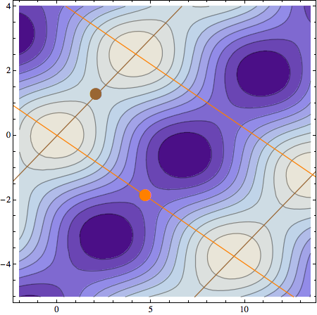
In Figure 1 we show one such domain, delimited by the lines and . The domain has the origin, with coordinates
| (19) |
in one of its corners (the other three corners are three equivalent minima of the potential). The central part of the domain is occupied by the maximum
| (20) |
Finally, each of the four sides contains a saddle point, with equivalent saddle points on opposite sides. We denote by and , respectively, the saddle point on the and on the line. These points are marked in Figure 1, and they have coordinates
| (21) |
Without loss of generality, we can restrict the initial conditions for the fields to be in this domain. Moreover - again due to the symmetry properties of the potential - we can restrict the initial conditions to be along the valley that ends on , or (when it exists) along a valley that starts from one of the two saddle points . Such valleys are shown in Figure 2 and are studied in Section III. Any other valley in the potential can be mapped to one of these valleys.
III Valleys and crests of the field potential
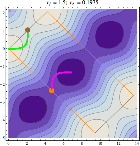
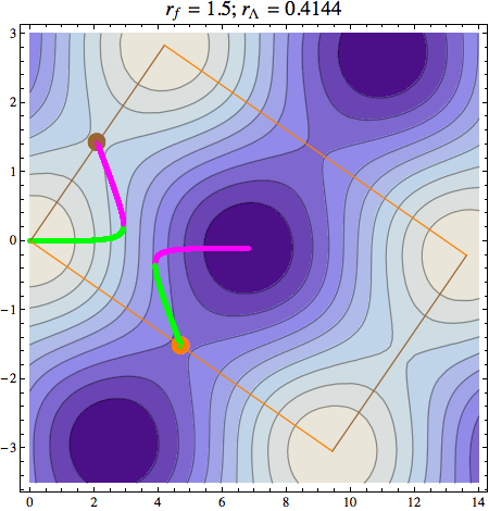
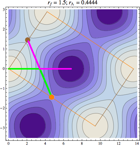
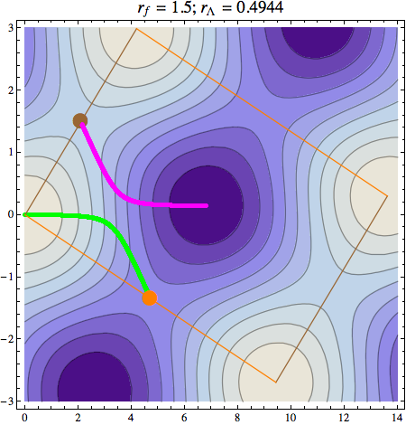
We study the valleys and crests of the potential (16); these are lines in the plane for which . The stable valleys minimize the potential in the direction (), while the unstable crests maximize it (). As discussed at the end of the previous Section, we restrict our attention to , and to valleys and crests that are (i) inside the domain we have singled out, and (ii) connected either to the origin or to one of the saddle points . The equipotential lines of Figure 2 show how the valleys and crests extend to other domains, or beyond the maximum . However, due to the symmetries of the potential, we do not need to consider these extension in the present discussion.
In general, we could not solve the condition analytically, so that we do not have general analytic expressions for the valleys and crests . However, it is straightforward to obtain such lines numerically. We summarize the result of our investigation in Figure 2, where valleys and crests are shown as green and magenta lines, respectively. The results summarized in the figure agree with the analytic results that we could obtain in neighborhoods of the extrema of the potential (the origin, the maximum, and the saddle points), and for the special case . This analytic results are reported in Appendix A, and they confirm the validity of what we present here. The valleys and crests have a qualitatively different behavior according to the relative value of vs . We discuss these different behaviors starting from small , and discussing how the lines change as increases.
For (top-left panel of Figure 2), a valley extends from the minimum to the saddle point , and a crest extends from the maximum to the saddle point . In the interval (top-right panel) we still find a first curve extending from the minimum to , and a second curve extending from the maximum to . However both curves are partially a stable valley and partially an unstable crest. For (bottom-left panel), the two curves join each other at a point. Finally, for (bottom-right panel), a stable valley extends from the origin to , while an unstable crest extends from the maximum to .
At , a reconnection between the two curves take place. Specifically, for (top two panels of Figure 2), a curve connects the origin with , and a curve connects the maximum with . Instead, for (bottom-right panel of Figure 2), the origin is connected with and the maximum with . A “swap” between two halves of the two curves takes place at , which is the only value of for which the two curves touch each other at a point.
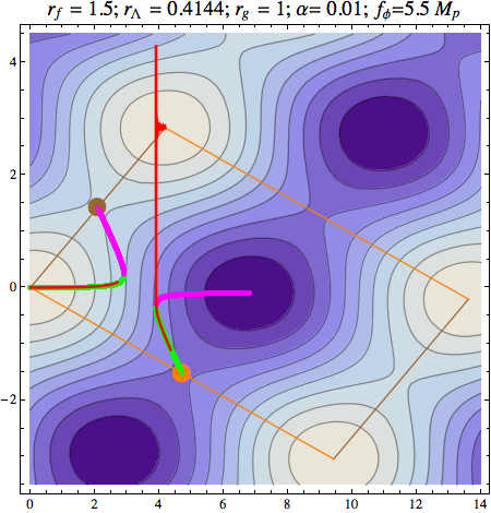
Provided the effective axion scale is sufficiently large, the valleys are inflationary attractors. The valleys shown in Figure 2 are obtained from the potential (16), where subdominant terms in the exact potential (6) are disregarded. We performed several numerical evolutions in the exact potential (6) for , and we verified that the valleys of Figure (2) describe the inflationary evolution with very good accuracy. Figure 3 shows two examples of this. We choose parameters in the interval, so that two distinct and inequivalent 777In the sense that the valleys cannot be mapped into each other by a symmetry of the potential, so they give a different phenomenology. valleys exist, one connected to the minimum at the origin, and one disconnected from it. The red curves in the figure show two inflationary trajectories obtained from the exact potential (6). These are two different inflationary evolutions for the same model and for the same choice of parameters, but with different initial conditions. As we discuss below, they lead to a different phenomenology.
The trajectory on the inflationary valley disconnected from the origin is particularly interesting. Inflation ends not because the potential reaches a minimum, but because the inflationary valley () becomes an unstable crest (, so that inflation is terminated by an instability in the heavy direction. We see in the figure that, after leaving the inflationary valley, the system reaches a new line; the heavy field performs damped oscillations about this valley, and eventually the system reaches the minimum on the top of the figure by evolving in the light direction. This stage of the evolution is very fast. The evolution shown in the figure is characterized by e-folds of inflation along the valley connected to ; the following phase, from the moment the system leaves the valley to when it first reaches the minimum, lasts for e-folds. During this second stage, the equation of state oscillates with average . This phase should be understood as the beginning of the post-inflationary reheating.
IV phenomenology
In this Section we study the CMB phenomenology of Aligned Natural Inflation in the plane. As discussed in the previous Section, we find two classes of inflationary trajectories in this model: those along valleys connected to a minimum, and those along valleys disconnected from any minimum. In the first case, inflation ends as the fields approach the minimum of the potential; in the second case inflation terminates at the end of the valley, due to an instability in the heavy direction. This second class of solutions exist only for in the interval. 888To be precise, such an evolution can also take place for slightly greater than , so that evolutions where inflation ends due to instability in the direction are possible for , with small. The reason for this is that, for , one finds at the precise point where the valley connects with the crest shown in the figure, so that the fields do not bend along the valley, but escape from it (ending inflation), and again reach the minimum shown on the top of the figure. This behavior rapidly disappears as increases slightly above , since all along the valley in this case. For the parameters used in Figure 3, we numerically found that (while ).
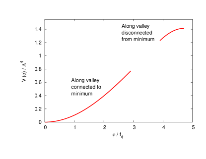
Significantly different phenomenological results are obtained in these two cases, and, for this reason, we discuss them in two separate subsections. We anticipate that the evolutions along valleys disconnected from minima lead to a significantly smaller value of the tensor-to-scalar ratio than the other trajectories, and of what is generically found in axion inflation. The reason for this is that the potential is flatter ( smaller parameter) closer to a saddle point than to a minimum (see Figure 4). We stress that the valleys disconnected from the minima are missed if one rotates the potential at the origin into a heavy and light direction at the origin, and he/she then makes the approximation that all of inflation takes place along the line.
We performed several inflationary evolutions for the model, with different values of the parameters, and we verified that the CMB phenomenology obtained from the field effective potential (18) is in very good agreement with that obtained from the exact model (6). In the plots shown below we have obtained the fields evolution from the exact model (6), and we have then computed the values of and using the slow-roll relations (70).
IV.1 Inflation on valleys connected to minima
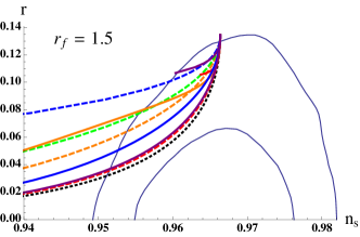
For definiteness, we computed the CMB phenomenology for the case in which the axion scales are all comparable to each other, and . We also fixed the alignment parameter to , and the number of e-folds of inflation to . We then varied to cover all the different cases shown in Figure 2. The results of our evaluations are shown in Figure 5. Each line shown in the Figure corresponds to a given value of and to varying .
All curves have a common end on the top-right part, corresponding to large . Figure 4 shows the potential along a connected valley as a function of . As grows, a given value of produces a longer inflationary expansion. Therefore, if is fixed to , one needs to decrease the value of as increases. At large , one is probing only the part of that is closest to the origin, where a quadratic approximation of the potential suffices. One then recovers the values of massive chaotic inflation, and .
As a comparison, the black dotted line in the figure refers to Natural Inflation Freese:1990rb . All the four dashed lines in the figure sample the model in the region. We see that the smallest value of shown gives results very close to Natural Inflation. This is explained by the analytic computation presented in Appendix A, where we show that Aligned Natural Inflation reproduces Natural Inflation in the limit of very small . We then see that increasing in this interval leads to progressively greater values of . This is particularly true in the left portion of the curves shown in the figure. As we mentioned above, the top-right part of the curves is obtained at relatively large , while decreases as one moves towards the left of the curves. As decreases, needs to start closer and closer to the saddle point. Eq. (38) gives the analytic form of the effective field potential close to this point. We see from this relation that increasing (in the regime that we are considering here) indeed results in a less flat potential, and so in a greater value of , in agreement with the dashed curves of the figure.
The two top solid theoretical curves shown in Figure 5 sample the regime. We recall that in this figure we only consider inflation in the valley connected to the minimum. We see from the top-right panel of Figure 2 that this valley becomes a crest before reaching a saddle point. For this reason, cannot be taken arbitrarily small, and, as a consequence, the corresponding curve in the plane only extends for a finite interval. The length of this interval decreases as we approach the value. This is due to the fact that also the fraction of the stable portion of the curve from to the minimum decreases as .
Finally, the three bottom solid theoretical curves shown in Figure 5 sample the region. At relatively small (left part of the curves), the evolution starts close to the saddle point . Eq. (40) shows that the potential becomes progressively flatter as increases in this regime. This explains the behavior of the three bottom solid curves in the figure. We see that the curve corresponding to the highest value of shown also approaches that of Natural Inflation. This is explained by the analytic computation presented in Appendix A, where we show that Aligned Natural Inflation reproduces Natural Inflation in the limit of very large .
We also performed computations for other values of , and we obtained results qualitatively similar to those of Figure 5. For brevity, we do not show them here.
IV.2 Inflation on valleys disconnected from minima
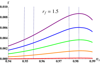
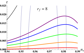
As we mentioned, in the interval, inflation can occur on valleys that are connected to the saddle point and that are disconnected from any minimum. Inflation ends because the heavy direction becomes unstable. The tensor-to-scalar ratio in these trajectories is significantly smaller than the one found for the valleys connected to a minimum. This is visible in the two Figures 6 and 7, where, respectively, the two cases and are studied (such values do not have any particular importance, and they have been chosen just as a representative case of comparable axion scales, or somewhat hierarchical axion scales).
It is possible to reproduce analytically the results shown in these two figures with good accuracy. Most of inflation occurs close to the saddle point, where the field effective potential reads
| (22) |
In this equation, we have defined (cf. eq. (40)),
| (23) |
while denotes the value of at which inflation ends (due to the fact that the orthogonal direction becomes tachyonic at that point). This is a top-hat potential with maximum on the saddle point (of the field potential) located at . The slow roll parameters on this potential are
| (24) |
Integrating the slow roll relation , one obtains the value of at e-folds before the end of inflation:
| (25) |
and finally, from the slow roll relations , one obtains the functional relation
| (26) |
Each theoretical curve in Figures 6 and 7 is obtained for fixed and , and for varying . The value of can be obtained from imposing along the inflationary trajectory, where the potential (16) is used. We see that any fixed value of and , results in a given value of . Therefore, each curve is characterized by the same value 999This is confirmed with very good accuracy by the numerical evolutions with the exact potential (6). of , so that (26) gives the prediction for the shape of the theoretical curves, up to an overall rescaling. A comparison with the exact numerical results shown in Figures 6 and 7 shows that (26) - with obtained from a numerical evolution with the exact field potential - is accurate up to a few percent level discrepancy for , while the discrepancy increases to level for .
We can have a fully analytic relation by estimating the value at which inflation vanishes. Eq. (39) is an analytic expression for the inflationary trajectory in the neighborhood of . We insert this expression in , expand to quadratic order in , and set this expression to zero. This provides a simple estimate for the value of at which the heavy direction becomes tachyonic:
| (27) |
We stress that this value cannot be extremely accurate, as it is obtained by expanding the potential close to , and not close to the where the instability occurs. Nonetheless, it provides a reasonable estimate. By comparing with the exact numerical evolutions used for Figures 6 and 7, we find that the estimate (27) is accurate up to discrepancy for , while the discrepancy increases to level as . Combining (26) and (27), one obtains
| (28) |
Despite not perfectly accurate, eq. (28) can be used to understand the behavior of with the parameters of the potential. For instance, it shows that, at any fixed , the value of grows with growing , in agreement with what is seen in Figures 6 and 7. It also shows that in general grows with (the derivative with respect to of the right hand side of (28), evaluated for the , is positive). This is also confirmed by the comparison between Figure 6 and Figure 7.
V Coupling to vector fields
The couplings of an axion to “matter” fields are highly constrained by the shift symmetry. The leading operators that give the coupling to gauge and fermion fields are, respectively, and , where is the axion scale, and where and are model dependent dimensionless coefficients that, in the spirit of an effective field theory, are naturally expected to be .
The coupling to gauge fields typically controls the perturbative decay of an axion inflaton after inflation, as the decay into fermions is helicity suppressed Pajer:2013fsa . Moreover, this coupling also leads to interesting gauge field production already during inflation. 101010These considerations are valid for any gauge field whose quanta are light during inflation. Although explicit computations in the literature assume U(1) fields, the results can be easily extended to the non-abelian case. See Pajer:2013fsa and Barnaby:2011vw for the details of the computations that we discuss in this section. Specifically, one gauge field helicity becomes tachyonic in presence of this operator Anber:2006xt , and the corresponding gauge quanta are non-perturbatively produced (this effect vanishes both in the UV regime and IR regime, so the production is “self-regulated”, and does not diverge). The amount of produced quanta 111111In this discussion we consider the production of gauge fields from the inflaton during inflation. See Barnaby:2011qe for a discussion and Adshead:2015pva for a more detailed study of the production at reheating. is exponentially sensitive to the parameter Anber:2006xt in the regime, while the production is negligible at (for definiteness, we assume to be positive in this discussion. Changing sign of simply changes the gauge helicity state that is produced, and so it does not change the phenomenological constraints). These gauge quanta inverse decay to produce inflaton perturbations, that are highly non-gaussian Barnaby:2010vf and that have a blue spectrum that can lead to too many primordial black holes Linde:2012bt . They can also produce gravity waves Barnaby:2011vw that violate parity Sorbo:2011rz , and that also have a blue spectrum, growing to a level that can be tested already at the next generation interferometer experiments Cook:2011hg ; Barnaby:2011qe ; Crowder:2012ik . All these effects constrain . The estimate of Linde:2012bt suggests that the limit from primordial black holes, that forces , is the strongest one, although the precise limit is sensitive to the evolution of the scalar perturbations in a highly nonlinear regime, which may not be fully under computational control Linde:2012bt . The other limits are more robust, and constrain Pajer:2013fsa . 121212The quantity typically increases during inflation. The limits quoted here refer to the value assumed by when the large CMB scales left the horizon. Using the slow roll relation , we can rewrite
| (29) |
and so we see that the regime is typically reached when Barnaby:2010vf .
Such effects may help in phenomenologically distinguishing the single field Natural Inflation from the Aligned Inflation mechanism. Indeed, as we now discuss, they are negligible in the former case, while they may be detectable in the latter case. To see this, consider the operators
| (30) |
where in the second line is the axion scale introduced in (5). The parameters are model-dependent dimensionless coefficients (for instance, such a coupling can arise from integrating out heavy fermions that couple both to the axion and to the gauge field), which may naturally be expected to be of order one. In the aligned inflation case, we use (12) to rotate to the base of light () and heavy field () during inflation, and we arrive to the coupling
| (31) |
where the scales and have been defined in (15), while, again, the parameters and are model-dependent dimensionless coefficients which may naturally be expected to be of order one. 131313These coefficients are related to those entering in (30) by and , up to corrections.
As we have discussed after eq. (15), the rescaled fields and exhibit a similar excursion during inflation. However, the original field moves much more than . This is encoded in the factor entering in (31): due to the greater excursion, the light field is coupled to the gauge field much more strongly than . So, the coupling of the inflaton to the gauge field in Natural Inflation and Aligned Natural Inflation is given, respectively, by
| (32) |
We therefore see that, in Natural Inflation, a value is necessary to produce a visible effect, in contrast to the natural expectation. Also in Aligned Natural Inflation, a value is required to have a visible effect. However, due to the enhancement, this can be possible even if .
In Figure 8 we show the required value of to produce in Aligned Natural Inflation, for the parameter choice . 141414Figure 8 has been obtained from the exact value of in numerical evolutions of the exact field model (6), with and . However, the same result can also be obtained from the effective field model (18), where the parameters and do not enter (one only requires that ). We observe that a stronger coupling is required for trajectories along valleys disconnected from minima of the potential, since the inflaton potential is flatter along those valleys (see the discussion at the beginning of Section IV).
To summarize, in Natural Inflaton the request of a sufficiently flat potential, namely , imposes a strong limit on the coupling strength of the inflaton to gauge fields, which precludes an interesting production of gauge quanta during inflation. On the contrary, if the aligned mechanism is employed, one can start from significantly smaller axion decay constants, and hence a significantly stronger coupling to gauge fields, and still obtain a flat inflaton potential, . The fact that none of the effects associated to the gauge field production has been yet observed translates into limits of the coupling of the axions to any light gauge field, and provides useful constrains for model building Barnaby:2011qe .
VI Conclusions
The alignment mechanism of Kim:2004rp has received considerable attention in the recent past. Despite of this, a detailed study of the inflationary trajectories in this model, and of the associated phenomenology, was still missing. The main goal of this work was to perform such a study. We were particularly interested in understanding whether the model can be phenomenologically distinguished from single field Natural Inflation. The prediction from Natural Inflation are outside the current CMB contours, and the model will be fully explored once the sensitivity to is reached Munoz:2014eqa , see for instance Figure 5. 151515In our figures, we fixed the number of e-folds of visible inflation to . Such a value is obtained for a quick reheating after Natural Inflation. Slower reheating (under the conventional assumption that the equation of state at reheating is smaller than that of radiation Podolsky:2005bw , ) implies that the large scale CMB perturbations were produced closer to the end of inflation (), when the potential was less flat. This gives a larger value of than the one shown in Figure 5. A number of current and near future CMB experiments have claimed sensitivity, and the current discussion of Stage 4 experiments aims to reach sensitivity Abazajian:2013vfg . It is therefore of particular interest to study whether Aligned Natural Inflation can provide values of below the dotted line shown in Figure 5, as this region cannot be covered by single field Natural Inflation.
The most interesting result emerged from our analysis is the existence of inflationary trajectories near saddle points of the potential, and disconnected from minima of the potential (in the sense that these trajectories end far away from minima, because the heavy field perpendicular to them becomes unstable). As studied in Section IV these trajectories lead to much smaller values of than those obtained in Natural Inflation. The prediction for the evolutions along these trajectories is given by eq. (28), which is a fully analytic expression in terms of the parameters in the model and of the number of e-folds. As we discussed, this relation is only an approximate one, but it is reasonably accurate, and it allows to understand the dependence of the phenomenological predictions on the parameters of the model.
A second possible way to distinguish Aligned Natural Inflation from single field Natural Inflation originates from the fact that a stronger coupling of the inflaton to other fields should be expected in the former, given that the starting axion scales are sub-Planckian. A moderate level of alignment, , is associated to axion scales, where the coupling of the axions to any massless or light () gauge field can lead to significant gauge field production during inflation, with several phenomenological consequences Pajer:2013fsa . We reviewed this in Section V.
Finally, we hope that the conclusions learnt from the present study can be of relevance also for other multi-field models of axion inflation. Recently, there has been considerable interest of inflation in the landscape of string theory, and on the relevance of critical points in multi-field inflationary potentials, see for instance Aazami:2005jf ; Frazer:2011tg ; Agarwal:2011wm ; Battefeld:2012qx ; Battefeld:2013xwa ; Marsh:2013qca . We have shown that the presence of critical points in one of the field extensions of Natural Inflation can strongly impact the phenomenological predictions of that model, and this may be the case also for other multi-field extensions that we have mentioned in this work. It may be interesting to perform a systematic study of trajectories, and explore the relevance of saddle points, also for such models.
Acknowledgements: The work of M.P. is partially supported from the DOE grant DE-SC0011842 at the University of Minnesota. The work of C.U. was partially supported by a summer grant from the graduate program of the School of Astronomy and Physics of the University of Minnesota.
Appendix A Analytic properties of the valleys and crests
In this Appendix, we denote as “curve” a line along which . Namely
| (33) |
These curves are stable valleys if , in which case they can support inflation provided that the effective axion scale is sufficiently large. They are instead unstable crests if .
Inserting the solution of (33) into the field potential provides the effective field potential, as formally described in eq. (18). In general, eq. (33) can be solved numerically. Here we discuss the cases for which we could obtain an analytic solution.
A.1 Critical points
The condition (33) is obviously satisfied at the critical points listed in Section II. We can therefore solve it analytically for small displacements about these points. Next to the origin we obtain
| (34) |
By computing , and imposing (34), we can verify that (34) is a stable valley (which is obvious, given that the origin is a minimum of ). We observe that, as the valley reaches the origin, vanishes faster than . This is due to the fact that, as we discussed after performing the rotation (12), the fields and are mass eigenvectors near the origin, so that the light field valley must proceed along at this point. We also see from (34) that, on the immediate right of the origin, the valley bends to positive for and to negative for . This can be seen, respectively, in the top two panels of Figure 2 and in the bottom right panel.
Being of , the field does not contribute to the quadratic potential near the origin, where we have
| (35) |
Near the maximum, namely for and , the condition (33) is solved by
| (36) |
This curve is unstable near . To the left of the maximum, this curve bends towards negative for and towards positive for . This is the opposite of the curve connected to the origin. As Figure 2 shows, when one curve connects the minimum with the saddle point at positive , the other curve connects the maximum with the saddle point at negative , and viceversa.
A.2
As discussed in the main text, at the interesting value of , a reconnection between the two curves takes place. For , the field enters in the two arguments of the two sine functions in (33) multiplied by the same coefficient . We could then solve (33) analytically, and find that the condition is satisfied by two straight lines: one joining the minimum with the maximum , and one joining the two saddle points and . The two lines intersect at the point , of coordinates
| (41) |
One can show analytically that only parts of the two curves are stable (): specifically, the segment between and the minimum , and the segment between and . The other parts of the trajectories are unstable.
Along the stable segment, the potential reads
| (42) |
and the argument of the cosine ranges from to as one moves from to along the trajectory.
Along the stable segment, the potential reads
| (43) |
and the argument of the sine ranges from to as one moves from to along the curve.
A.3
We recall that the potential (16) is invariant under the simultaneous exchanges and . For this reason, we do not need to discuss the case . In the main text we studied the case . Here we discuss the case. The main difference with the discussion of the main text is that now the regime is absent.
For , the field enters with the same coefficient in the two potential terms. Thanks to this, we can write
where
| (45) |
For , one finds and . Therefore, the condition leads to the two curves (a straight line connecting the minimum to the maximum ), and (a straight line connecting the two saddle points). Along the first curve, the potential reads , and so the trajectory is stable in its first half close to the minimum). Along the second curve, the potential is constant, , and . This can be understood as the limit of the case shown in the bottom-left panel of Figure 2.
Let us now discuss the case. We write the solutions of as the two curves satisfying
| (46) |
The curve with the sign connects the minimum with the saddle point for , and with the saddle point for . 161616We recall that the model is symmetric under and . In the current case, , the symmetry identifies with . We see that the saddle points interchange role in this identification. In both cases the variable ranges from to , and the effective potential along the trajectory evaluates to
| (47) |
Since the potential is always , the curve is a stable valley (see eq. (LABEL:rf1-AB)).
The curve with the sign instead connects the maximum to the saddle point for , and with the saddle point for . This curve in an unstable crest. The behavior and the stability of the two curves agree with those discussed in the main text for (cf. the top-left panel of Figure 2 for , and the bottom-right panel of Figure 2 for ), showing that the limit is continuous.
A.4 Very small or large
These are the regimes in which one term in the potential (6) is strongly dominant over the other term. The condition sets this term to a negligible value. Then one is left with the other term, evaluated along the trajectory set by the first term. This reproduces the potential of Natural Inflation.
To be specific, the very small (respectively, large) regime requires (respectively, ). We start the discussion with the very small regime. In this limit, the left hand side of eq. (33) can vanish only if the the argument of the first sine is at most of . This implies
| (48) |
and, as a consequence, the argument of the second sine in eq. (33) is . Using this information in the potential (16), we learn that
| (49) |
Namely, up to negligible corrections,
| (50) |
A completely analogous computation shows that
| (51) |
Appendix B Cosmological perturbations in the field model
We start by computing the cosmological scalar perturbations for a generic model of two canonically normalized real scalar fields, characterized by the action
| (52) |
We work in conformal time and in spatially flat gauge:
| (53) |
Moreover, we decompose the scalar fields as a dependent background component plus perturbations
| (54) |
We insert (53) and (54) into the starting action, and obtain the quadratic order action in the perturbations . We then integrate out the non-dynamical fields and . 171717The fields and enter in without time derivatives, and so they do not add any extra dynamical degree of freedom. It is customary (see for instance Maldacena:2002vr ) to integrate them out (i) by evaluating the constraint equations , (ii) by solving them expressing the nondynamical variables and in terms of the dynamical variables and , and (iii) by inserting these expressions back into the action . In this way becomes an action in terms of the dynamical fields only. Doing so, one obtains
| (55) |
where , and prime denotes differentiation with respect to . We note that the variables are the canonical variables of the problem, and that their conjugate momenta are
| (56) |
We further decompose the Fourier modes into mode functions times annihilation/creation operators:
| (57) |
The mode functions satisfy the classical equations of motion
| (58) |
where is the identity operator, and the squared mass matrix defined in (55). To quantize the system, we impose standard Equal Time Commutation Relations among the fields and their conjugate variables, and the standard algebra on the annihilation/creation operators:
| (59) |
To ensure these relations, we impose
| (60) |
at some given initial time . The first condition in (60) ensures that both relations (59) can be imposed at . Enforcing all three of (60) at ensures that these conditions continue to hold at later times (as can be immediately verified taking their time derivatives and using (58)). This ensures that the first relation in (59) holds at all times.
We impose the initial conditions when a mode is deeply inside the horizon. Specifically, the physical momentum should dominate the dispersion relation of the mode. The entries in the mass matrix (55) are of , where are the two mass eigenvalues of . Therefore, we ensure that . Neglecting slow roll corrections, during inflation, and so we impose
| (61) |
Using this approximated expression for , we see that the equations of motion (58) admit the early time solution . So, we impose,
| (62) |
which satisfy all three of (60). Namely, in the deep sub-horizon regime the mass matrix is irrelevant, and the two eigenmodes of the system behave as decoupled massless modes in Minkowski space-time. The solution just written is the standard adiabatic vacuum solution for these decoupled modes.
We are interested in observables that are linear in the two scalar fields, , where the (real) coefficients can depend on background quantities (and, hence, on time). We assume that we have a set of such observables , so that
| (63) |
and we compute the two point correlation function among pairs of them
where we have used the fact that (thanks to statistical isotropy) the mode functions do not depend on the direction of , and where we have introduced the power spectra
| (65) |
(we note that this expression is symmetric and real).
In shorts, for any set of observables (63), we compute the self- and cross-power spectra by imposing the initial conditions (62), by evolving (58), and by evaluating (65).
In this work, we have two scalar fields and , and we are interested in the power in the adiabatic and entropy modes, that, in spatially flat gauge, read (see Malik:2008im for a review)
| (66) |
where we have defined
| (67) |
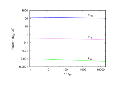
The solid lines of Figure (9) show the auto- and cross- spectra of the adiabatic and entropy modes for an illustrative choice of parameters, with inflation taking place along the high-altitude plateau connected to the saddle point . The adiabatic mode corresponds to perturbations along the light inflationary direction, while the entropy mode corresponds to the much heavier orthogonal direction (the alignment parameter is ). As expected, the entropy mode is significantly smaller than the adiabatic one, and we can simply disregard it, with very good accuracy. Starting from the quadratic action (55), performing the rotation (66), and setting , we obtain the theory for the single perturbation, in the limit in which can be disregarded. As expected, we explicitly verified that, in this limit, the quadratic action for reproduces that of a single field with a potential equal to the potential of the field model along the inflationary trajectory. Specifically, setting , we obtain
| (68) |
which is the standard action Mukhanov:1990me for the Mukhanov-Sasaki variable Mukhanov:1985rz ; Sasaki:1986hm in the single field case.
One may then use the standard slow roll relations for the perturbations,
| (69) |
with the slow roll parameters evaluated along the inflationary trajectory
| (70) |
The dotted line in Figure 9 shows the power spectrum for obtained through the slow-roll relation (69), with the slow roll parameter evaluated through (70). This differs by about from the exact result indicated by the solid line. The discrepancy is consistent with the accuracy of the slow-roll approximation (in this run, ).
Appendix C An incorrect simplification ()
In this Appendix we warn against a simplification that in general provides incorrect phenomenological results. The transformation (12) rotates (up to negligible corrections) the original axions and of the starting potential (6) into the linear combinations and . Such fields are, respectively, the light and heavy directions of the inflaton potential close to the minimum at . For this reason, the inflationary evolution next to the origin occurs along the direction. One therefore may be tempted to simply set all throughout inflation. This would lead to the single field potential (16) with .
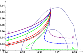
In Figure 10 we show with dashed lines the phenomenological results obtained under this incorrect assumption, for four different choices of parameters. As a comparison, we also show with solid lines the correct phenomenological results, obtained from an exact numerical evolution. We see that the approximated results shown are in reasonable agreement with the correct ones only in the top part of the lines, where is greatest.
Each line is obtained by varying only and keeping the other parameters constant. The common point of all the lines corresponds to . In this limit, only probes the immediate vicinity of the minimum, where the model becomes identical to massive chaotic inflation (in practice, only the first quadratic term of the Taylor expansion of the potential around the minimum matters). As setting is a good approximation close to the minimum, the approximate dashed lines approach the correct solid lines in that limit. However, as decreases, the system probes the potential far from minima, where the assumption is incorrect. This explains why setting does generally not provide the correct phenomenological results for the model.
References
- (1) P. A. R. Ade et al. [Planck Collaboration], arXiv:1502.02114 [astro-ph.CO].
- (2) D. H. Lyth, “What Would We Learn by Detecting a Gravitational Wave Signal in the Cosmic Microwave Background Anisotropy?,” Phys. Rev. Lett. 78 (1997) 1861 [hep-ph/9606387].
- (3) K. Freese, J. A. Frieman and A. V. Olinto, Phys. Rev. Lett. 65, 3233 (1990).
- (4) F. C. Adams, J. R. Bond, K. Freese, J. A. Frieman and A. V. Olinto, Phys. Rev. D 47, 426 (1993) [hep-ph/9207245].
- (5) E. Pajer and M. Peloso, Class. Quant. Grav. 30, 214002 (2013) [arXiv:1305.3557 [hep-th]].
- (6) N. Arkani-Hamed, H. C. Cheng, P. Creminelli and L. Randall, Phys. Rev. Lett. 90, 221302 (2003) [hep-th/0301218].
- (7) N. Arkani-Hamed, H. C. Cheng, P. Creminelli and L. Randall, JCAP 0307, 003 (2003) [hep-th/0302034].
- (8) D. E. Kaplan and N. J. Weiner, JCAP 0402 (2004) 005 [hep-ph/0302014].
- (9) F. Paccetti Correia, M. G. Schmidt, Z. Tavartkiladze and , Nucl. Phys. B 739, 156 (2006) [hep-th/0504083].
- (10) J. E. Kim, H. P. Nilles and M. Peloso, JCAP 0501, 005 (2005) [hep-ph/0409138].
- (11) S. Dimopoulos, S. Kachru, J. McGreevy and J. G. Wacker, JCAP 0808, 003 (2008) [hep-th/0507205].
- (12) A. R. Liddle, A. Mazumdar and F. E. Schunck, Phys. Rev. D 58, 061301 (1998) [astro-ph/9804177].
- (13) E. Silverstein and A. Westphal, Phys. Rev. D 78, 106003 (2008) [arXiv:0803.3085 [hep-th]].
- (14) L. McAllister, E. Silverstein and A. Westphal, Phys. Rev. D 82, 046003 (2010) [arXiv:0808.0706 [hep-th]].
- (15) S. Hannestad, T. Haugbolle, P. R. Jarnhus and M. S. Sloth, JCAP 1006, 001 (2010) [arXiv:0912.3527 [hep-ph]].
- (16) F. Marchesano, G. Shiu and A. M. Uranga, JHEP 1409, 184 (2014) [arXiv:1404.3040 [hep-th]].
- (17) K. Harigaya and M. Ibe, Phys. Lett. B 738, 301 (2014) [arXiv:1404.3511 [hep-ph]].
- (18) L. McAllister, E. Silverstein, A. Westphal and T. Wrase, JHEP 1409, 123 (2014) [arXiv:1405.3652 [hep-th]].
- (19) T. Li, Z. Li and D. V. Nanopoulos, arXiv:1409.3267 [hep-th].
- (20) R. Blumenhagen, D. Herschmann and E. Plauschinn, arXiv:1409.7075 [hep-th].
- (21) Q. E. Minor and M. Kaplinghat, arXiv:1411.0689 [astro-ph.CO].
- (22) A. Hebecker, P. Mangat, F. Rompineve and L. T. Witkowski, arXiv:1411.2032 [hep-th].
- (23) R. Flauger, L. McAllister, E. Silverstein and A. Westphal, arXiv:1412.1814 [hep-th].
- (24) T. Li, Z. Li and D. V. Nanopoulos, arXiv:1412.5093 [hep-th].
- (25) I. Garc a-Etxebarria, T. W. Grimm and I. Valenzuela, arXiv:1412.5537 [hep-th].
- (26) R. Blumenhagen, A. Font, M. Fuchs, D. Herschmann and E. Plauschinn, arXiv:1503.01607 [hep-th].
- (27) S. Mohanty and A. Nautiyal, Phys. Rev. D 78, 123515 (2008) [arXiv:0807.0317 [hep-ph]].
- (28) M. M. Anber and L. Sorbo, Phys. Rev. D 81, 043534 (2010) [arXiv:0908.4089 [hep-th]].
- (29) L. Visinelli, JCAP 1109, 013 (2011) [arXiv:1107.3523 [astro-ph.CO]].
- (30) A. Albrecht, R. Holman and B. J. Richard, arXiv:1412.6879 [hep-th].
- (31) A. Berera, Phys. Rev. Lett. 75, 3218 (1995) [astro-ph/9509049].
- (32) N. Kaloper and L. Sorbo, Phys. Rev. Lett. 102, 121301 (2009) [arXiv:0811.1989 [hep-th]].
- (33) N. Kaloper, A. Lawrence and L. Sorbo, JCAP 1103, 023 (2011) [arXiv:1101.0026 [hep-th]].
- (34) E. Dudas, JHEP 1412, 014 (2014) [arXiv:1407.5688 [hep-th]].
- (35) C. Germani and A. Kehagias, Phys. Rev. Lett. 106, 161302 (2011) [arXiv:1012.0853 [hep-ph]].
- (36) P. Adshead and M. Wyman, Phys. Rev. Lett. 108, 261302 (2012) [arXiv:1202.2366 [hep-th]].
- (37) A. Maleknejad and M. M. Sheikh-Jabbari, Phys. Lett. B 723, 224 (2013) [arXiv:1102.1513 [hep-ph]].
- (38) E. Dimastrogiovanni and M. Peloso, Phys. Rev. D 87, no. 10, 103501 (2013) [arXiv:1212.5184 [astro-ph.CO]].
- (39) P. Adshead, E. Martinec and M. Wyman, Phys. Rev. D 88, no. 2, 021302 (2013) [arXiv:1301.2598 [hep-th]].
- (40) R. Namba, E. Dimastrogiovanni and M. Peloso, JCAP 1311, 045 (2013) [arXiv:1308.1366 [astro-ph.CO]].
- (41) I. Obata, T. Miura and J. Soda, arXiv:1412.7620 [hep-ph].
- (42) J. Ohashi and S. Tsujikawa, JCAP 1210, 035 (2012) [arXiv:1207.4879 [gr-qc]].
- (43) D. Maity, Phys. Lett. B 720, 389 (2013) [arXiv:1209.6554 [hep-th]].
- (44) M. Czerny and F. Takahashi, Phys. Lett. B 733, 241 (2014) [arXiv:1401.5212 [hep-ph]].
- (45) M. Czerny, T. Higaki and F. Takahashi, JHEP 1405, 144 (2014) [arXiv:1403.0410 [hep-ph]].
- (46) R. Kallosh, A. Linde and B. Vercnocke, Phys. Rev. D 90, 041303 (2014) [arXiv:1404.6244 [hep-th]].
- (47) T. C. Bachlechner, M. Dias, J. Frazer and L. McAllister, arXiv:1404.7496 [hep-th].
- (48) G. Shiu, W. Staessens and F. Ye, arXiv:1503.01015 [hep-th].
- (49) G. Shiu, W. Staessens and F. Ye, arXiv:1503.02965 [hep-th].
- (50) J. McDonald, arXiv:1407.7471 [hep-ph].
- (51) J. McDonald, arXiv:1412.6943 [hep-ph].
- (52) D. Croon and V. Sanz, JCAP 1502, no. 02, 008 (2015) [arXiv:1411.7809 [hep-ph]].
- (53) D. Croon, V. Sanz and J. Setford, arXiv:1503.08097 [hep-ph].
- (54) C. P. Burgess, M. Cicoli, F. Quevedo and M. Williams, JCAP11(2014)045 [arXiv:1404.6236 [hep-th]].
- (55) C. Csaki, N. Kaloper, J. Serra and J. Terning, Phys. Rev. Lett. 113, 161302 (2014) [arXiv:1406.5192 [hep-th]].
- (56) A. de la Fuente, P. Saraswat and R. Sundrum, arXiv:1412.3457 [hep-th].
- (57) T. Rudelius, arXiv:1503.00795 [hep-th].
- (58) M. Montero, A. M. Uranga and I. Valenzuela, arXiv:1503.03886 [hep-th].
- (59) J. Brown, W. Cottrell, G. Shiu and P. Soler, arXiv:1503.04783 [hep-th].
- (60) T. C. Bachlechner, C. Long and L. McAllister, arXiv:1503.07853 [hep-th].
- (61) A. Hebecker, P. Mangat, F. Rompineve and L. T. Witkowski, arXiv:1503.07912 [hep-th].
- (62) N. Arkani-Hamed, L. Motl, A. Nicolis and C. Vafa, JHEP 0706, 060 (2007) [hep-th/0601001].
- (63) S.-H. H. Tye and S. S. C. Wong, arXiv:1404.6988 [astro-ph.CO].
- (64) R. Kappl, S. Krippendorf and H. P. Nilles, Phys. Lett. B 737, 124 (2014) [arXiv:1404.7127 [hep-th]].
- (65) A. Chatzistavrakidis, E. Erfani, H. P. Nilles and I. Zavala, JCAP 1209, 006 (2012) [arXiv:1207.1128 [hep-ph]].
- (66) K. Choi, H. Kim and S. Yun, Phys. Rev. D 90, 023545 (2014) [arXiv:1404.6209 [hep-th]].
- (67) T. Higaki and F. Takahashi, JHEP 1407, 074 (2014) [arXiv:1404.6923 [hep-th]].
- (68) T. Higaki and F. Takahashi, arXiv:1409.8409 [hep-ph].
- (69) K. Y. Choi, J. E. Kim and B. Kyae, arXiv:1410.1762 [hep-th].
- (70) M. Berg, E. Pajer and S. Sjors, Phys. Rev. D 81, 103535 (2010) [arXiv:0912.1341 [hep-th]].
- (71) I. Ben-Dayan, F. G. Pedro and A. Westphal, arXiv:1404.7773 [hep-th].
- (72) C. Long, L. McAllister and P. McGuirk, Phys. Rev. D 90, 023501 (2014) [arXiv:1404.7852 [hep-th]].
- (73) X. Gao, T. Li and P. Shukla, JCAP 1410, no. 10, 048 (2014) [arXiv:1406.0341 [hep-th]].
- (74) T. Li, Z. Li and D. V. Nanopoulos, JHEP 1411, 012 (2014) [arXiv:1407.1819 [hep-th]].
- (75) I. Ben-Dayan, F. G. Pedro and A. Westphal, arXiv:1407.2562 [hep-th].
- (76) C. D. Carone, J. Erlich, A. Sensharma and Z. Wang, arXiv:1410.2593 [hep-ph].
- (77) T. Ali, S. S. Haque and V. Jejjala, arXiv:1410.4660 [hep-th].
- (78) T. C. Bachlechner, C. Long and L. McAllister, arXiv:1412.1093 [hep-th].
- (79) R. Kappl, H. P. Nilles and M. W. Winkler, arXiv:1503.01777 [hep-th].
- (80) F. Ruehle and C. Wieck, arXiv:1503.07183 [hep-th].
- (81) R. Kallosh, Lect. Notes Phys. 738, 119 (2008) [hep-th/0702059 [HEP-TH]].
- (82) L. McAllister and E. Silverstein, Gen. Rel. Grav. 40, 565 (2008) [arXiv:0710.2951 [hep-th]].
- (83) C. P. Burgess, M. Cicoli and F. Quevedo, JCAP 1311, 003 (2013) [arXiv:1306.3512 [hep-th]].
- (84) D. Baumann and L. McAllister, arXiv:1404.2601 [hep-th].
- (85) R. Blumenhagen and E. Plauschinn, Phys. Lett. B 736, 482 (2014) [arXiv:1404.3542 [hep-th]].
- (86) A. Hebecker, S. C. Kraus and L. T. Witkowski, Phys. Lett. B 737, 16 (2014) [arXiv:1404.3711 [hep-th]].
- (87) T. W. Grimm, Phys. Lett. B 739, 201 (2014) [arXiv:1404.4268 [hep-th]].
- (88) Z. Kenton and S. Thomas, arXiv:1409.1221 [hep-th].
- (89) A. Westphal, arXiv:1409.5350 [hep-th].
- (90) H. Abe, T. Kobayashi and H. Otsuka, arXiv:1409.8436 [hep-th].
- (91) A. Mazumdar and P. Shukla, arXiv:1411.4636 [hep-th].
- (92) D. F. Chernoff and S.-H. H. Tye, arXiv:1412.0579 [astro-ph.CO].
- (93) C. Burgess and D. Roest, arXiv:1412.1614 [hep-th].
- (94) A. D. Linde, Phys. Rev. D 49, 748 (1994) [astro-ph/9307002].
- (95) N. Barnaby and M. Peloso, Phys. Rev. Lett. 106, 181301 (2011) [arXiv:1011.1500 [hep-ph]].
- (96) N. Barnaby, R. Namba and M. Peloso, JCAP 1104, 009 (2011) [arXiv:1102.4333 [astro-ph.CO]].
- (97) M. M. Anber and L. Sorbo, JCAP 0610, 018 (2006) [astro-ph/0606534].
- (98) N. Barnaby, E. Pajer and M. Peloso, Phys. Rev. D 85, 023525 (2012) [arXiv:1110.3327 [astro-ph.CO]].
- (99) P. Adshead, J. T. Giblin, T. R. Scully and E. I. Sfakianakis, arXiv:1502.06506 [astro-ph.CO].
- (100) A. Linde, S. Mooij and E. Pajer, Phys. Rev. D 87, no. 10, 103506 (2013) [arXiv:1212.1693 [hep-th]].
- (101) L. Sorbo, JCAP 1106, 003 (2011) [arXiv:1101.1525 [astro-ph.CO]].
- (102) J. L. Cook and L. Sorbo, Phys. Rev. D 85 (2012) 023534 [Erratum-ibid. D 86 (2012) 069901] [arXiv:1109.0022 [astro-ph.CO]].
- (103) S. G. Crowder, R. Namba, V. Mandic, S. Mukohyama and M. Peloso, Phys. Lett. B 726, 66 (2013) [arXiv:1212.4165 [astro-ph.CO]].
- (104) J. B. Munoz and M. Kamionkowski, Phys. Rev. D 91, no. 4, 043521 (2015) [arXiv:1412.0656 [astro-ph.CO]].
- (105) D. I. Podolsky, G. N. Felder, L. Kofman and M. Peloso, Phys. Rev. D 73, 023501 (2006) [hep-ph/0507096].
- (106) K. N. Abazajian, K. Arnold, J. Austermann, B. A. Benson, C. Bischoff, J. Bock, J. R. Bond and J. Borrill et al., Astropart. Phys. 63, 55 (2015) [arXiv:1309.5381 [astro-ph.CO]].
- (107) A. Aazami and R. Easther, JCAP 0603, 013 (2006) [hep-th/0512050].
- (108) J. Frazer and A. R. Liddle, JCAP 1102, 026 (2011) [arXiv:1101.1619 [astro-ph.CO]].
- (109) N. Agarwal, R. Bean, L. McAllister and G. Xu, JCAP 1109, 002 (2011) [arXiv:1103.2775 [astro-ph.CO]].
- (110) D. Battefeld, T. Battefeld and S. Schulz, JCAP 1206, 034 (2012) [arXiv:1203.3941 [hep-th]].
- (111) D. Battefeld and T. Battefeld, JCAP 1307, 038 (2013) [arXiv:1304.0461 [hep-th]].
- (112) M. C. D. Marsh, L. McAllister, E. Pajer and T. Wrase, JCAP 1311, 040 (2013) [arXiv:1307.3559 [hep-th]].
- (113) J. M. Maldacena, JHEP 0305, 013 (2003) [astro-ph/0210603].
- (114) K. A. Malik and D. Wands, Phys. Rept. 475, 1 (2009) [arXiv:0809.4944 [astro-ph]].
- (115) V. F. Mukhanov, H. A. Feldman and R. H. Brandenberger, Phys. Rept. 215, 203 (1992).
- (116) V. F. Mukhanov, JETP Lett. 41, 493 (1985) [Pisma Zh. Eksp. Teor. Fiz. 41, 402 (1985)].
- (117) M. Sasaki, Prog. Theor. Phys. 76, 1036 (1986).