Fermion Masses and Mixing in General Warped Extra Dimensional Models

Abstract

We analyze fermion masses and mixing in a general warped extra dimensional model, where all the Standard Model (SM) fields, including the Higgs, are allowed to propagate in the bulk. In this context, a slightly broken flavor symmetry imposed universally on all fermion fields, without distinction, can generate the full flavor structure of the SM, including quarks, charged leptons and neutrinos. For quarks and charged leptons, the exponential sensitivity of their wave-functions to small flavor breaking effects yield naturally hierarchical masses and mixing as it is usual in warped models with fermions in the bulk. In the neutrino sector, the exponential wave-function factors can be flavor-blind and thus insensitive to the small flavor symmetry breaking effects, directly linking their masses and mixing angles to the flavor symmetric structure of the 5D neutrino Yukawa couplings. The Higgs must be localized in the bulk and the model is naturally more successful in generalized warped scenarios where the metric background solution is different than $AdS_{5}$. We study these features in two simple frameworks, flavor complimentarily, and flavor democracy, which provide specific predictions and correlations between quarks and leptons, testable as more precise data in the neutrino sector becomes available.

I Introduction

The discovery of a SM-like Higgs boson at the LHC with a mass of 125 GeV was a huge step forward in confirming the validity of the Standard Model (SM) and probing the electroweak symmetry breaking mechanism. But despite its experimental success, the SM still fails to provide an explanation, among other things, for the origin and observed pattern of fermion masses and mixings.

In the quark sector, the masses are extremely hierarchical, with the top much heavier than the rest of the quarks and with a strong ordering. In the up sector, the masses are separated by three orders of magnitude, while in the down sector the mass ratios are separated by two orders of magnitude. The quarks also exhibit mixing patterns given by three small mixing angles and a large (CP) phase. In the lepton sector, the charged lepton masses obey a similar hierarchical pattern as the down-type quarks. On the other hand, though not known exactly, neutrino masses are known to be very small and their square mass differences imply a closer mass pattern, $\Delta m_{31(32)}^{2}:\Delta m_{21}^{2}\sim 10^{2}:1$. Neutrinos appear to mix maximally and this has been long-seen as pointing towards a different flavor origin between quarks and leptons, and also to the necessity of introducing new physics. After the successful measurement of the neutrino mixing angle $\theta_{13}$ by the Daya Bay An:2012eh ; An:2013uza , T2K Abe:2011sj ; Abe:2014ugx , MINOS Adamson:2011ig ; Adamson:2014vgd , RENO Ahn:2012nd and Double Chooz Abe:2012tg ; Abe:2014bwa Collaborations, the determination of the neutrino mass hierarchy has become a priority for theoretical studies and for future neutrino experiments. A great deal of theoretical work in this area has been trying to provide answers, based on such diverse frameworks as see-saw mechanisms Minkowski:1977sc ; Supergravity:GellMann80 ; Yanagida79 ; Glashow80 ; Mohapatra:1979ia ; Schechter:1980gr ; Lazarides:1980nt , Abelian Frampton:2002yf ; Lavoura:2004tu ; Dev:2010if and non-Abelian Lam:2008rs ; Lam:2008sh ; Grimus:2009pg ; Ge:2011ih ; He:2011kn ; Toorop:2011jn ; Ge:2011qn ; deAdelhartToorop:2011re ; He:2012yt ; Hernandez:2012ra ; Lam:2012ga ; Hernandez:2012sk ; Holthausen:2012wt ; Hu:2012ei ; Hernandez:2013vya ; King:2013vna ; Hagedorn:2013nra ; Lavoura:2014kwa symmetries imposed on the leptonic sector (both charged and neutral), and many texture structures for leptonic mass matrices, including modifications of accepted paradigms, such as tri-bimaximal Harrison:1999cf ; Harrison:2002er ; Xing:2002sw ; Harrison:2002kp ; Harrison:2003aw ; He:2003rm , bi-maximal Vissani:1997pa ; Barger:1998ta ; Baltz:1998ey ; Stancu:1999ct ; Georgi:1998bf ; Li:2004nh and democratic Fritzsch:1995dj ; Fritzsch:1998xs ; Fritzsch:1999im neutrino mixing matrices. While various attempts to unify the description of quarks and leptons already exist (mostly based on quark-lepton complementarity Zhang:2012pv ; Zhang:2012zh ; Li:2011ag ; Kang:2011tv ; Ahn:2011yj ; Shimizu:2010pg ; Patel:2010hr ; Barranco:2010we ; Zheng:2010kp ; Xing:2009eg ; Frampton:2008ep ; Rodejohann:2008zz ; Plentinger:2007px ; Picariello:2007ss ), an attractive possibility would be that quarks and leptons obey the same symmetry at a higher scale, which is then slightly broken at lower scales, yielding different patterns for masses and mixing for the quarks/leptons than for the neutrinos. This is the scenario we plan to investigate here, in the context of warped extra dimensions, where small symmetry breaking terms have very different effects on quarks and leptons due to the geometry of the model.

Introducing a warped extra dimension provides an elegant way to address both the hierarchy problem (to stabilize the Higgs mass against large radiative corrections) and the fermion flavor hierarchy problem. These models were first proposed to deal with the hierarchy problem of the SM Randall:1999ee ; Randall:1999vf , where introducing an extra dimension produced a five dimensional anti-de Sitter ($AdS_{5}$) geometry bounded by two hard walls (branes) along the extra dimension, referred to as the Planck (or UV) brane and the TeV (or IR) brane. Allowing for exponential modulation from the gravity scale down to the weak scale along this compact extra dimension Randall:1999ee ; Randall:1999vf , naturally yields the weak-Planck mass hierarchy.

The original Randall-Sundrum (RS) model localized all SM fields on the IR brane, leading to severe flavor violation bounds on the new physics scale. It was later shown that if the fermions were allowed to propagate in the bulk of the extra dimension Grossman:1999ra ; Gherghetta:2000qt ; Davoudiasl:1999tf ; Chang:1999nh ; Casagrande:2010si ; Huber:2003tu , the same model could address the flavor hierarchy problem of the SM as well. The model thus emerged as a geometric theory of flavor. By localizing the Higgs on the IR brane with anarchic order-one couplings to the bulk fermions, the profiles of the fermion zero-modes can be adjusted to reproduce the observed Yukawa couplings in the low energy theory. Since the first and second generation fermions are localized towards the UV brane, they inherit substantial flavor protection from the RS-GIM mechanism Agashe:2004cp . However, by allowing the SM fields to propagate in the bulk, from an effective 4D point of view, a tower of KK fermions exists for all the SM fields, yielding enhanced contributions to electroweak and flavor observables in the SM Agashe:2003zs ; Burdman:2002gr ; Burdman:2003nt ; Huber:2003tu ; Carena:2004zn ; Carena:2003fx ; Delgado:2007ne ; Agashe:2004cp ; Quiros:2013yaa . This effect imposes a stringent bound on the scale of new physics of some $\sim 10$ TeV Csaki:2008zd ; Agashe:2008uz and hence renders these models completely out of the reach of current experiments. Some solutions were proposed to relieve these restrictions. One way was to extend the gauge symmetry of the model by introducing an $SU(2)_{R}$ gauge sector with custodial protection Agashe:2006at ; Huber:2003tu ; Agashe:2003zs . Here the basic idea is to align the down-type Yukawa couplings using the additional symmetry, so that the primary sources of intergenerational mixing are the up-type Yukawa couplings. Since the dominant constraints on FCNCs come from the down-type sector, the constraint on KK masses is substantially relaxed. A different approach to address the issue is through a slight modification of the warping factor along the extra dimension, allowing it to deviate slightly from the $AdS_{5}$ metric Falkowski:2008fz ; Batell:2008me ; MertAybat:2009mk ; Cabrer:2009we ; Cabrer:2010si ; Cabrer:2011fb . This deviation is such that the warping is more drastic near the TeV brane, while the background becomes more $AdS_{5}$-like near the Planck brane. These type of metric solutions can help suppress dangerous contributions to the electroweak and flavor observables by reducing the constraints on new physics down to about $\sim 1$ TeV.

Warped extra dimensional models were shown to provide new contributions to the Higgs production rate through gluon fusion which could conflict with the collider data Casagrande:2010si ; Azatov:2010pf ; Frank:2013un ; Frank:2013qma .

Interestingly, in the modified 5D metric scenarios the region of parameter space in which the dangerous contributions to flavor and electroweak precision observables are small is the same as the region where the new contributions to the Higgs production cross section are also small (and thus safe) Frank:2013qma . Moreover, this is achievable only when the Higgs field in these models is allowed to leak considerably into the bulk.

In the context of warped extra dimensional models with ${\cal O}(1)$ 5D Yukawa couplings and with no a priori structure (i.e., flavor anarchy), one can easily generate the hierarchical structure of the quark and charged lepton sectors Csaki:2008qq while, due to large mixing angles, the neutrino sector must be treated differently. In particular, in Agashe:2008fe , it was shown that if the Higgs field leaks sufficiently into the bulk it is possible that the (exponentially small) neutrino wave functions become independent on the flavor structure of the 5D neutrino mass parameters ($c^{i}_{\nu}$), and thus the 4D neutrino flavor structure depends directly on the flavor structure of the 5D neutrino Yukawa couplings.

In a previous work Frank:2014aca , we proposed a unified picture of fermion masses and mixings in the context of a warped extra dimensional model with $AdS_{5}$ background metric, and with all the SM fields in the bulk, including the Higgs. In that picture, the same flavor symmetric structure is imposed on all the fermions of the SM, including neutrinos. Small flavor breaking effects are exponentially enhanced in the quark and charged lepton sectors, thus producing hierarchical masses and mixings. With a sufficiently delocalized Higgs field, the neutrino wave functions are flavor-blind and the flavor structure is governed by the 5D neutrino Yukawa flavor structure.

In this work, we revisit this idea in the context of the modified $AdS_{5}$ metric solutions. We show that the SM masses and mixing can be generated successfully, and the mass generation in the neutrino sector appears to be more natural than in the case where a pure $AdS_{5}$ background metric is assumed.

Our work is organized as follows. We summarize the features of the modified $AdS_{5}$ model in Section II, with particular emphasis on fermion mass generation. We explore an explicit implementation of the scenario, flavor complementarity, in Section III and another, of a democratic flavor symmetry, in Section IV. We summarize our results and conclude in Section V. We leave the details of some calculations for the Appendix VI.

II Fermion masses in warped space

We consider a 5D warped space with the extra dimension compactified and allow all SM fields to propagate in the following generalized warped space-time metric:

$$ds^{2}=e^{-2A(y)}\eta_{\mu\nu}dx^{\mu}dx^{\nu}-dy^{2},$$ (1)

$\eta_{\mu\nu}={\rm diag}(-1,1,1,1)$ being the flat metric. The 5-th dimension, $y$, is bounded by two branes localized at $y=0$ and $y=y_{1}$ and $A(y)$ is a model-dependent function. As mentioned in the Introduction, some generalized warped models can be safe from precision electroweak tests and flavor bounds for very low KK masses. Motivated by this, we consider a modified $AdS_{5}$ scenario with the following warp exponent Cabrer:2010si ; Carmona:2011rd :

$$A(y)=ky+\frac{1}{\nu^{2}}\ln\left(1-\frac{y}{y_{s}}\right),$$ (2)

where $k\sim M_{Pl}$ is the $AdS_{5}$ curvature, expected to be of the order of the Planck mass scale, $y_{s}$ is the position of the metric singularity, always chosen to be outside of the physical region, $y_{s}>y_{1}$, and $\nu>0$ is a model parameter taken to be real. The $\nu$ parameter, alongside $\Delta=y_{s}-y_{1}$, the distance between the location of the metric singularity and the IR brane, measures the departure of the metric from the pure $AdS_{5}$ background. The smaller the values of $\Delta$ and $\nu$, the more modified the metric; intuitively, the singularity has a larger effect on the physics at the IR brane the closer it gets to it. One can calculate the curvature along the 5-th dimension and obtain

$$R(y)=8A^{\prime\prime}(y)-20\left(A^{\prime}(y)\right)^{2}.$$ (3)

The curvature radius, $L(y)=\sqrt{-20/R}$, in units of $k$ along the 5-th dimension is then given by

$$kL(y)={k\Delta\over\sqrt{1-2\nu^{2}/5+2\nu^{2}k\Delta+(\nu^{2}k\Delta)^{2}}}.$$ (4)

One can see that for values of $\nu>\sqrt{5/2}$, this function has a minimum before the singularity and therefore the curvature can change sign within the physical region. Following Cabrer:2011fb , we impose that this minimum is located outside of the physical region and hence the curvature radius is a monotonically decreasing function between the UV and the IR branes.

The more familiar RS metric is recovered by taking the limits $\nu\rightarrow\infty$ and $y_{s}\rightarrow\infty$, yielding $A(y)=ky$, with the curvature radius being constant, $kL=1$.

Figure 1: The modified $AdS_{5}$ warp factor $A(y)$ versus the standard RS warp exponent, $y$. The horizontal line corresponds to $ky=35$. For the same amount of warping, the modified scenario requires a shorter length scale along the 5-th dimension.

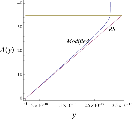
In Figure 1, we compare the two metrics and plot the warp exponent function $A(y)$ for the $AdS_{5}$ and the modified $AdS_{5}$ cases. We can see that the amount of warping near the IR brane at around $ky=35$ is larger for the modified $AdS_{5}$. Thus, as the figure indicates, the same amount of warping from the UV brane to the IR brane in the modified scenario requires a slightly smaller length of the 5-th dimension and hence an IR brane slightly closer to the UV brane. The curvature radius (Eq. 4) at the UV brane is approximately equal for the pure and modified $AdS_{5}$ spaces with, $ky(y)\simeq 1$. In contrary, at the IR brane, as $kL(y)$ is a monotonically decreasing function, $ky(y)$ assumes its minimal value for the modified $AdS_{5}$ space and hence $kL_{1}\equiv kL(y_{1})$ is a good measure of the amount of deviation from the pure $AdS_{5}$ space with constant curvature radius.

The 5D fermion Lagrangian density with Dirac neutrinos is

$${\cal L}_{q} = {\cal L}_{kinetic}+M_{q_{i}}{\bar{Q}_{i}}Q_{i}+M_{u_{i}}{\bar{U}_{i}}U_{i}+M_{d_{i}}{\bar{D}_{i}}D_{i}+(Y^{u\,5D}_{ij}H\bar{Q}_{i}U_{j}+h.c.)$$ (5)

$$+(Y^{d\,5D}_{ij}H\bar{Q}_{i}D_{j}+h.c.)+(Q_{i}\!\!\rightarrow\!\!L_{i},U_{i}\!\!\rightarrow\!\!N_{i},D_{i}\!\!\rightarrow\!\!E_{i})\,,$$

where, $i,j$ are flavor indices and the 5D Yukawa parameters, $Y_{ij}^{5D}$, are dimension-full quantities of ${\cal O}(1)\times\sqrt{k}$. $Q_{i}$ ($L_{i}$) are 5D quark (lepton) fields for $SU(2)$ doublets while $U_{i}$ ($N_{i}$) and $D_{i}$ ($E_{i}$) are $SU(2)$ singlet quark (lepton) fields. The bulk mass, $M_{\psi_{i}}$, originating from the momentum along the 5-th dimension, can be taken in general to be $y$-dependent. To be able to compare, we choose it such that it coincides with its usual definition in RS models, and express it in units of the 5-th dimension curvature, $k$, as $M_{\psi_{i}}=c_{\psi}^{i}k$, where $c_{\psi}^{i}$ are localization parameters, dimensionless quantities of ${\cal O}(1)$, and $\psi_{i}$ runs over all SM quarks and leptons. Dimensional reduction then yields the normalized profile for the fermion and the Higgs fields along the bulk of the extra dimension, $q^{0,i}_{L}(y)$, $u^{0,i}_{R}(y)$ and $h(y)$, which are given by

$$q^{0,i}_{L}(y) = q^{i}_{0}\ e^{(2-c_{q}^{i})A(y)}\,,$$ (6)

$$u^{0,i}_{R}(y) = u^{i}_{0}\ e^{(c_{u}^{i}+2)A(y)}\,,$$ (7)

$$h(y) = h_{0}\ e^{aky}\,,$$ (8)

with $q^{i}_{0}=f(c_{q}^{i})$, $\ u^{i}_{0}=f(-c_{u}^{i})\$ and $\ h_{0}=e^{-(a-1)ky_{s}}\mathfrak{h}_{0}$, and where $f(c)$ and $\mathfrak{h}_{0}$ are normalization factors which depend on $c$, $\nu$ and $y_{s}$, given explicitly in Appendix VI, along with their limiting expressions for the usual RS ($AdS_{5}$) metric background. From these profiles, one can check that localization of the fields in the bulk of the extra dimension is determined by the values of the $c_{\psi}^{i}$ for the fermion fields, such that a value of $c_{\psi}^{i}>1/2$ indicates a UV localized field, while a value of $c_{\psi}^{i}<1/2$ localizes the field near the IR brane. The Higgs field localization along the 5-th dimension is given by the parameter $a$, the dimension of the Higgs condensate operator. A completely IR brane localized field corresponds to the limit $a\rightarrow\infty$, while for a delocalized Higgs field $a$ is small. However, in order to maintain the original Randall-Sundrum solution to the hierarchy problem without fine-tuning, the Higgs field localization should be such that $a\mathrel{\raise 1.29167pt\hbox{$>$\kern-7.5pt\lower 4.30554pt\hbox{$\sim$}}}2$ (for an $AdS_{5}$ metric background). If the 5D Higgs potential is of the form $V_{bulk}(H)=M_{5d}^{2}H^{2}$, with associated brane potentials at each boundary, the Higgs profile has two solutions, one growing towards the IR and another one decaying at the IR brane. This last one is proportional to $e^{(4-a)ky}$ in the $AdS5$ background. In order to maintain the RS solution to the hierarchy problem, the decaying solution has be subdominant, and this happens naturally for $a>2$. For $a<2$, some fine-tuning between the parameters of the bulk scalar potential and the brane potentials is necessary in order to suppress the unwanted solution. In the modified $AdS_{5}$ scenario the lowest value of $a$ that does not require fine-tuning depends on the various new metric parameters Quiros:2013yaa . In this case, the Higgs profile is given by

$$h(y)=h_{0}e^{aky}\bigg{[}1+(M_{0}/k-a)\left[F(y)-F(0)\right]\bigg{]},$$ (9)

where $M_{0}$ is the brane Higgs mass term (coefficient of the $|H|^{2}\delta(y-y_{1})$ term at the IR brane) and the function $F(y)$ is given by

$$F(y)=e^{-2(a-2)ky_{s}}ky_{s}\left[-2(a-2)ky_{s}\right]^{-1+4/\nu^{2}}\Gamma\left[1-\frac{4}{\nu^{2}},-2(a-2)k(y_{s}-y)\right].$$ (10)

The decaying term at the IR brane is the second term in Eq. (9) and, forcing $M_{0}/k\simeq a$ (fine-tuning parameters), the solution can become sub-dominant. In order to avoid this fine-tuning of parameters, we note that as $F(y)$ is a monotonically increasing function, and if one has $\delta\equiv|F(y_{1})|\sim{\cal O}(1)$, no fine-tuning is needed to guarantee that the increasing solution for the Higgs profile dominates. When the parameter $\delta=F(y_{1})$ becomes larger, this solution needs fine-tuning of parameters to suppress its value. Fig. 2 shows the no-fine-tuning region (above the red solid $\delta=1$ curve) in the $(a,\nu)$ plane, where $a$ is the Higgs localization parameter and $\nu$ is the metric parameter of the modified metric solution. The region below is the one fine-tuned, requiring an adjustment of Lagrangian parameters with a tuning precision growing exponentially. (The close dashed curve locates the points where $\delta=10$, i.e. where the tuning is already 10 $\%$) .

In producing these graphs, for each case we first set the value of the IR brane position, $ky_{1}$, which in turn fixes the value of $y_{s}$, the position of the singularity. Then for each value of the parameter $\nu$ we solved for $a$ in $\delta(a,\nu,y_{1},y_{s})=1$.

$\begin{array}[]{cc}\includegraphics[width=170.71652pt,height=199.16928pt]{aVSnuplotp2.pdf}&\hskip 17.07182pt\includegraphics[width=170.71652pt,height=199.16928pt]{aVSnuplotp99.pdf}\end{array}$

Figure 2: The $\delta=1$ plots and the connection with neutrino masses in the $\nu-a$ plane for (left panel) $kL_{1}=0.2$ (large deviation) and (right panel) $kL_{1}=0.99$ (more RS-like). The red (solid) curve locates the no-fine-tuning threshold in which $\delta=1$. Above this curve, $\delta<1$, and below the curve, $\delta>1$ (corresponding to the unwanted fine-tuned region). The shaded area corresponds to a heavy neutrino mass ($m_{3}$ in normal ordering), $m_{\nu}\sim 5\times 10^{-11}$ GeV for different values of the $c$-parameters, but such that the mass expression has no exponential sensitivity to the $c$-parameters. Note that in the RS-like case (right panel) it is not possible to obtain neutrino masses without fine-tuning, or quitting the neutrino plateau parameter region (as would be the case in usual RS scenarios). With modified-$AdS_{5}$ metric (left panel) it is possible to find non-tuned points with neutrino masses in the plateau (corresponding to no exponential $c$-dependence).

To first order, the effective SM Yukawa couplings are obtained from the overlap integral

$$y_{ij}^{u}=\frac{Y^{u}_{ij}}{\sqrt{k}}\int_{0}^{y_{1}}dye^{-4A(y)}h(y)q^{0,i}_{L}(y)u^{0,j}_{R}(y)\,,$$ (11)

where the index $u$ denotes the four types of Yukawa couplings of the SM, i.e. $u=u,d,e,N$ and we have defined the dimensionless 5D Yukawa couplings as $Y_{ij}^{u}=Y^{5D}_{ij}/\sqrt{k}\sim{\cal O}(1)$. Given the profiles (6), (7) and (8) and the metric (2), the integral above can be performed analytically and written as

$$y_{ij}^{u}=\tilde{Y}_{ij}^{u}h_{0}f(c_{q}^{i})f(-c_{u}^{j}),$$ (12)

where the factor $\tilde{Y_{ij}^{u}}$, defined in Appendix VI, has very mild $c^{i}$ dependence. The function $f(c)$ is such that depending on the value of $c$, the Yukawa couplings can be exponentially sensitive to $c$, or only mildly dependent. Finally $h_{0}$ is the bulk Higgs normalization factor and does not depend on the fermion mass parameters $c^{i}$. Note that, although throughout the paper we have suppressed the explicit dependence of the fields on the metric parameters, $\nu$, $y_{s}$, $y_{1}$ and $k$, and in particular all of the factors of Eq. (12), are metric dependent. As shown in Appendix VI, one can always retrieve the RS limit for these terms by taking the limit $\nu,y_{s}\rightarrow\infty$.

$\begin{array}[]{cc}\includegraphics[height=199.16928pt]{fcContourRS1.pdf}&\includegraphics[height=199.16928pt]{fcRS2.pdf}\\ \end{array}$

(a) RS with all SM fields including the Higgs in the bulk, $a=2.04$ and $\delta=1$.

$\begin{array}[]{cc}\includegraphics[height=199.16928pt]{fcContour1.pdf}&\includegraphics[height=199.16928pt]{fc2.pdf}\\ \end{array}$

(b) Modified $AdS_{5}$ with $\nu=0.32$, $kL(y_{1})=0.2$, $A(y_{1})=35$, $a=4.46$ and $\delta=1$.

Figure 3: Effective 4D Yukawa couplings for fermions as functions of the fermion bulk mass parameter $c$ for (a) the RS and (b) general warped space-time metric. The plots in the right-hand side are produced by taking the $c$-parameters for the doublet and the singlet to be equal. In the left-handed plots, each contour depicts one order of magnitude difference with respect to its adjacent contour. A typical location for neutrino masses of order $m_{\nu}\sim 10^{-11}$ GeV is also shown. The shaded vertical band shows the region where all fermions of the SM should be located.

The fermion masses are given, to first order, by the eigenvalues of the $3\times 3$ Yukawa matrices of the form

$$v\ y^{u}=v\left(\begin{array}[]{ccc}y_{11}^{u}&y_{12}^{u}&y_{13}^{u}\\ y_{21}^{u}&y_{22}^{u}&y_{23}^{u}\\ y_{31}^{u}&y_{32}^{u}&y_{33}^{u}\end{array}\right).$$ (16)

In general, in order to get the correct SM masses, no exponential $c$-dependence is needed for the top quark, which corresponds to $c_{q}^{t}\mathrel{\raise 1.29167pt\hbox{$<$\kern-7.5pt\lower 4.30554pt\hbox{$\sim$}}}1/2$ and $c_{u}^{t}>-1/2$ (this region of parameter space corresponds to the top plateau shown in Fig. 3). For the rest of the SM particles $c_{q}^{i}\mathrel{\raise 1.29167pt\hbox{$>$\kern-7.5pt\lower 4.30554pt\hbox{$\sim$}}}1/2$ and $c_{u}^{i}<-1/2$, which implies that the Yukawa couplings will depend exponentially on the values of the $c^{i}$. In the case of neutrinos however, in order to accommodate their tiny masses, one needs localization parameters $c_{\nu}<-1$. It was shown Agashe:2008fe that, for a delocalized Higgs with $a$-parameter small compared to the localization parameter $c^{i}$, the 4D effective neutrino masses depend exponentially on $a$ but loose their dependence on the $c^{i}$’s. This region of parameter space corresponds to the neutrino plateau shown in Fig. 3. In other words, the limit of the function in Eq. (12) for large $c_{\nu}$-s is given by

$$y_{ij}^{u}\sim{\tilde{Y}_{ij}^{u}}h_{0}.$$ (17)

To make this more transparent, in the formula for fermion masses given by (cf.  Eq.(12))

$$(M_{f})_{ij}=v\tilde{Y}_{ij}^{u}h_{0}f(c_{q}^{i})f(-c_{u}^{j}),$$ (18)

we factor the exponential behaviors and write them in the following two distinct limits

$$(M_{f})_{ij} \sim vY_{ij}^{f}\epsilon^{(c_{q}^{i}-\frac{1}{2})}\epsilon^{-(c_{u}^{j}+\frac{1}{2})}\ \ \text{for}\ \ \ \ \ \ \ c_{q}>1/2,c_{u}<-1/2\,,$$

$$(M_{\nu})_{ij} \sim vY_{ij}^{N}e^{-ky_{1}(a-1)}\ \ \ \,\ \ \ \ \text{for}\ \ \ \ \ \ \ \ \ \ \ c_{q}-c_{u}>a\,,$$ (19)

where $\epsilon=e^{-A(y)}$ (see Appendix VI for details).

The limits described in Eq. (II) imply that, as the quark and charged lepton mass matrix elements are exponentially dependent on the $c^{i}$ parameters, any structure in the 5D Yukawa matrix elements $Y^{f}_{ij}$ will be largely washed-out and will always produce generically hierarchical fermion masses as well as small mixing angles. For the neutrinos, on the other hand, since there is no exponential sensitivity on the flavorful $c^{i}$ parameters, any structure inherent in the 5D Yukawa matrix elements will survive in the 4D effective theory. This is the region of neutrino parameter space we are interested in, shown in Fig. 3 as the neutrino plateau. In RS models, the actual height of the neutrino plateau is determined exclusively by the value of the $a$ parameter. For the value of the warp factor required to solve the hierarchy problem, the highest possible neutrino masses in the plateau are too small by 1-2 orders of magnitude (without fine-tuning) to be phenomenologically viable (see upper panels in Fig. 3). Some tuning, or some enhancement of the 5D Yukawa couplings, and/or trespassing the edge of the plateau would then be required, making the scenario less attractive for our purposes. On the other hand, in modified $AdS_{5}$ scenarios, although the level of the plateau is still highly sensitive to the value of $a$, the masses could actually be increased by some two orders of magnitude and thus allow for phenomenologically acceptable neutrino masses in the desired region of the model (see Fig. 2 and lower panels in Fig. 3). This feature occurs because the modified $AdS_{5}$ metric (see Eq. (2)) exhibits a richer parameter space. In the RS metric, in order to produce the correct neutrino masses in the plateau, we need $a\sim 1.85$, value which amounts to about $1/10000$ fine tuning of parameters in the 5D Higgs potential. While for modified $AdS_{5}$ scenarios, one can produce a neutrino plateau within the experimental bounds for some range of $a$ parameter values without fine-tuning. It is interesting that the parameter space for which the neutrino plateau is most favorable coincides with the region where small KK masses satisfy bounds coming from flavor and electroweak precision measurements Cabrer:2011qb ; deBlas:2012qf and constraints from Higgs phenomenology Frank:2013un .

$\begin{array}[]{cc}\includegraphics[width=199.16928pt,height=199.16928pt]{mnuVSnu22.pdf}&\includegraphics[width=199.16928pt,height=199.16928pt]{mnuVSnu11.pdf}\end{array}$

Figure 4: (Left panel) Neutrino masses as functions of the metric parameter $\nu$ for different values of the Higgs localization parameter $a$ and fixed $kL_{1}=0.2$. The fermion mass parameters ($c$’s) are fixed to a region where there is no exponential dependence on them (the neutrino plateau). The curves end whenever the fine-tuning threshold ($\delta=1$) is reached (thick overlapping curve). Note that for small values of $\nu$ the neutrino masses become larger while still remaining in the non-tuned regime and in the neutrino plateau. (Right panel) Same plot for different values of $kL_{1}$ and fixed $\delta=1$. The graph corresponding to $kL_{1}=0.9$ remains constant at larger values of $\nu$ and (approximately) coincides with the RS limit.

In order to further illustrate this issue, in Fig. 4 we show the resulting neutrino masses in the plateau region as a function of the parameter $\nu$, for different values of $a$ (left panel) and $kL_{1}$ (right panel). The area below the curves is the no-fine-tuning region, and one can see that the largest neutrino masses (in the plateau) occur for $\nu\sim 0.3$ and $kL_{1}=0.2$, whereas in the RS limit, i.e. $kL_{1}\sim 1$ and $\nu$ large, the masses are some two orders of magnitude lower (slightly too low). This makes the extended metric scenarios a more natural framework for the flavor mechanism investigated here, and adds to the advantages of these scenarios (i.e. a much lower KK scale consistent with electroweak and flavor bounds, and with Higgs production).

Qualitatively the general features of the flavor structure of these modified $AdS_{5}$ models are very similar to these features in the pure $AdS_{5}$ models for the bulk mass $c_{\psi}^{i}$ parameters. Therefore, in order illustrate our flavor setup, it is useful to consider the simpler case of the RS metric. In this case the fermion mass formulas Eq. (II), can be simplified dramatically. As usual, we consider the mass matrix for the neutrino sector separately from the case of quarks and charged leptons mass matrices. Consider the case with $c_{q,u}^{i}>\frac{1}{2}$. In this case we have,

$$(M_{f})_{ij} \simeq v\epsilon^{(c_{q}^{i}-\frac{1}{2})}\epsilon^{-(c_{u}^{j}+\frac{1}{2})}\sqrt{2(a-1)|1-2c_{q}^{i}||1+2c_{u}^{j}|}\tilde{Y}_{ij}^{f}$$

$$(M_{\nu})_{ij} \simeq v\epsilon^{a-1}\frac{\sqrt{2(a-1)|1-2c_{l}^{i}||1+2c_{\nu}^{j}|}}{\sqrt{\epsilon^{(1-2c_{l})}-1)}\sqrt{\epsilon^{(1+2c_{\nu})}-1}}\tilde{Y}_{ij}^{\nu},$$ (20)

where the 5D Yukawa couplings are given by,

$$\tilde{Y}_{ij}^{u}\simeq\frac{1}{a-c_{q}^{i}+c_{u}^{j}}Y_{ij}^{u}.$$ (21)

From Eq. (6), (7) and (11) one can see that there are two sources of flavor structure: the 5D dimensionless Yukawa couplings $Y^{u}_{ij}$, and the bulk mass coefficients $c_{\psi}^{i}$. We are interested in scenarios in which all Yukawa matrices ($Y_{F}=$ $Y^{u}_{ij}$, $Y^{d}_{ij}$, $Y^{\nu}_{ij}$, and $Y^{e}_{ij}$) and fermion bulk mass matrices from the 5D Lagrangian (${\mathbf{c}}_{f}=$ ${\mathbf{c}}_{q}$, ${\mathbf{c}}_{u}$, ${\mathbf{c}}_{d}$, ${\mathbf{c}}_{l}$, ${\mathbf{c}}_{\nu}$, and ${\mathbf{c}}_{e}$) share the same symmetry structure, which is then slightly broken through some high energy mechanism according to

$$Y_{F}=Y^{0}_{F}+\delta Y_{F},$$ (22)

$${\mathbf{c}}_{f}={\mathbf{c}}_{f}^{0}+\delta{\mathbf{c}}_{f},$$ (23)

where the matrices $Y_{F}^{0}$ and ${\mathbf{c}}_{f}^{0}$ are flavor symmetric while the perturbation matrices $\delta Y_{F}$ and $\delta{\mathbf{c}}_{f}$ are random. Inserting these perturbations in Eqs. (II), the fermion masses receive corrections to leading order as follows

$$m_{t}\ = \ m^{0}_{t}+\delta m_{t}\hskip 193.47882ptc_{q}^{3},c_{u}^{3}<1/2\,,$$

$$(m_{f})_{ij} = (m_{f})^{0}_{ij}\ f(\delta c_{q}^{i})f(\delta c_{u}^{j}))\sim(m_{f})^{0}_{ij}\ \epsilon^{(\delta c_{q}^{i}+\delta c_{u}^{j})}\hskip 45.52458pta>c_{l}^{i}+c_{u}^{j}\,,$$ (24)

$$(m_{\nu})_{ij} = (m_{\nu})^{0}_{ij}+\delta(m_{\nu})_{ij}\hskip 162.18062pta<c_{l}^{i}+c_{\nu}^{j}\ .$$

Therefore the same exponential sensitivity on the bulk mass $c_{\psi}^{i}$ parameters, $\epsilon\sim 10^{-15}$, responsible for producing the SM hierarchy in the standard RS, is now translated into exponential sensitivity of the symmetry breaking terms. As a consequence, small symmetry breaking terms ($|\delta c^{i}|\sim 0.1$) can produce mass corrections of order $10^{-15(\delta c^{i}+\delta c^{j})}$ (i.e., a hierarchy of order $\sim 10^{6}$) to the quark and charged lepton mass matrices. This is in complete agreement with the observed hierarchy in these sectors. As mentioned before, the neutrinos and the top quark fields live in the two plateaus (see Fig. 3) with mild $c_{\psi}^{i}$ sensitivity.

For the mixing angles, the eigenvectors matrix that diagonalizes the neutrino sector should be very close to the eigenvectors matrix of the 5D Yukawa matrix. However, in the quark and charged lepton sectors the mixing matrices are generically close to the unit matrix with off-diagonal entries hierarchically small as:

$$V_{L}^{u}\simeq\left(\begin{array}[]{ccc}1&\frac{f^{1}_{q}(\tilde{M_{u}})_{21}}{f^{2}_{q}(\tilde{M_{u}})_{11}}&\frac{f^{1}_{q}(\tilde{Y_{u}})_{13}}{f^{3}_{q}(\tilde{Y_{u}})_{33}}\\ -\frac{f^{1}_{q}(\tilde{M_{u}^{*}})_{21}}{f^{2}_{q}(\tilde{M_{u}^{*}})_{11}}&1&\frac{f^{2}_{q}(\tilde{Y_{u}})_{23}}{f^{3}_{q}(\tilde{Y_{u}})_{33}}\\ \frac{f^{1}_{q}(\tilde{M_{u}^{*}})_{31}}{f^{3}_{q}(\tilde{M_{u}^{*}})_{11}}&-\frac{f^{2}_{q}(\tilde{Y_{u}^{*}})_{23}}{f^{3}_{q}(\tilde{Y_{u}^{*}})_{33}}&1\end{array}\right),$$ (25)

where $f_{q}^{i}$ is shorthand for the profile functions $f(c_{q}^{i})$, $(\tilde{M_{u}})_{ij}$ is the $(ij)$ minor of the matrix in parenthesis, and $(\tilde{Y}_{u})_{ij}$ is the $ij$ element of the Yukawa matrix. We define the CKM and the PMNS matrices as the following

$$V_{CKM}\equiv V_{L}^{u}V_{L}^{d\dagger}\ \ \ \ \ \ \ \ \ \ \text{and }\ \ \ \ \ \ \ \ \ V_{PMNS}\equiv V_{L}^{\nu}V_{L}^{e\dagger}\ .$$ (26)

As mentioned after Eq. (II), for the quarks and charged leptons, the off-diagonal mixing angles are also exponentially sensitive to the $c_{\psi}^{i}$ parameters and hence to the small symmetry breaking terms. The $V^{f}_{L}$ matrix elements in Eq. (25) can then be written as

$$(V_{L}^{u,d,e})_{ij}\sim(V_{L}^{u,d,e})_{ij}^{0}\ \epsilon^{(\delta c_{q}^{i}-\delta c_{q}^{j})}\ \ \ \ \ \ \ \ \ \ \ \ \ \ \text{(\ for u, d and e) }\,,$$ (27)

where $(V_{L}^{u,d,e})_{ij}^{0}$ are the matrix elements before the flavor symmetry breaking and $\{i,j\}$ can be $\{1,2\}$, $\{1,3\}$ and $\{2,3\}$. We see again that, due to exponential warping, all original symmetries present in the high energy theory are washed out in the quark and charged lepton sectors. Contrary to this, in the Dirac neutrino sector, the terms in the $V_{L}^{\nu}$ are much less sensitive to the symmetry breaking terms, since their own dependence on the $c_{\psi}^{i}$ is mild in the region of parameters of interest. If we define the eigenvalues of the 5D neutrino Yukawa matrix as

$$Y_{\nu}^{diag}=V_{Y_{L}}Y_{\nu}V_{Y_{R}},$$ (28)

then the matrix diagonalizing the 4D effective neutrino mass matrix

$$(V_{L}^{\nu})_{ij}\sim(V_{Y_{L}})_{ij}\ .$$ (29)

So far the framework is general, and we did not specify the type of symmetry imposed. In the next two sections we will consider two concrete implementations, one within flavor complementarity and then a second within flavor democracy. The background metric considered will always be the modified $AdS_{5}$ solution, in the most favorable region of parameter space.

III Flavor complementarity

In the first symmetry implementation, in this section we study the effects of enforcing a strong correlation between 5D quark and 5D lepton parameters. This scenario is motivated by the observation that charged lepton masses and down quark masses obey similar patterns. In warped space models, masses are obtained from exponentially small overlap integrals, and having similar mass patterns can indicate that both the 5D Yukawa structure and the 5D bulk fermion masses ($c$-parameters) are very similar for the down quarks and for the charged leptons. We therefore assume that $Y_{d}=Y_{e}$ and ${\bf c}_{q}={\bf c}_{l}$ to a high order of precision, so that the differences in observed masses between down quarks and charged leptons come from deviations in the right handed bulk parameters ${\bf c}_{d}$ and ${\bf c}_{e}$.

At the same time, inspired by neutrino phenomenology, we l implement a popular 2-3 ($\mu-\tau$) symmetry Ma:2001mr ; Grimus:2001ex ; Mohapatra:2004hta ; Mohapatra:2005ra ; Nasri:2005gw ; Mohapatra:2006un ; Mohapatra:2006pu ; Xing:2006xa ; Ahn:2006nu ; Aizawa:2005yy ; Fuki:2006ag ; Joshipura:2005vy ; Grimus:2009pg ; Adhikary:2009kz ; Xing:2010ez ; Ge:2010js ; deMedeirosVarzielas:2011tp ; He:2011kn ; Gupta:2013it ; Adhikary:2013bma ; Adhikary:2012mt ; Liao:2012xm ; Hamzaoui:2013twa ; Lashin:2013xha within the general flavor structure of the model. We require that all the 5D Yukawa matrices must be symmetric under 2-3 permutations and consider, for simplicity, the case where the 5D fermion bulk mass matrices ${\bf c}_{f}^{0}$ are diagonal and degenerate in that basis (maybe a remnant of some global $U(3)$ flavor symmetry broken in the Yukawa sector), i.e.

$${\bf c}^{0}_{f}=\!\!\left(\begin{array}[]{ccc}{c^{\,0}_{f}}&0&0\\ 0&c^{\,0}_{f}&0\\ 0&0&c^{\,0}_{f}\end{array}\right),\ \ \ \ \ \$$ (33)

where $c^{0}_{f}$ are real parameters, and $f$ denotes both doublets and singlets $f=q,l,u,d,e,\nu$. In 4D scenarios, discrete permutation symmetries of the neutrino mass matrix are known to lead to interesting (and phenomenology viable) neutrino masses and mixing patterns (such as the tri-bimaximal mixing matrix Harrison:1999cf ; Harrison:2002er ; Xing:2002sw ; Harrison:2002kp ; Harrison:2003aw ; He:2003rm , or the bi-maximal mixing matrix Vissani:1997pa ; Barger:1998ta ; Baltz:1998ey ; Stancu:1999ct ; Georgi:1998bf ; Li:2004nh ).

We will impose the 0-th order Yukawa matrices to be

$$Y^{0}_{u,\nu}=y_{u}\left(\begin{array}[]{ccc}\sqrt{6}d&0&0\\ d&d+1&d-1\\ d&d-1&d+1\end{array}\right)\ \ {\rm and}\ \ \ \ Y^{0}_{d,e}=y_{d}\left(\begin{array}[]{ccc}a&1&1\\ c&g&e\\ c&e&g\end{array}\right),\ \ \ \ \ \$$ (40)

where the parameters $y_{u}$, $y_{d}$, $a$, $c$, $d$, $g$ and $e$ are complex. As explained above, we impose the down type Yukawa couplings to match the charged lepton ones, i.e. $Y_{d}=Y_{e}\equiv Y_{d,e}$. We further require that the up-type Yukawa couplings be the same as the neutrino Yukawa couplings, i.e $Y_{u}=Y_{\nu}\equiv Y_{u,\nu}$, in order to reduce free parameters and enhance the degree of correlation between quarks and leptons.

The structure of the down-type Yukawa $Y^{0}_{d,e}$ is set only by the 2-3 symmetry, but the structure of neutrino-type Yukawa couplings $Y^{0}_{u,\nu}$ in Eq. (40) requires more explanation. The number of parameters has been reduced to two complex parameters, $y_{u}$ and $d$, such that the rotation matrix that diagonalizes $Y^{0}_{\nu}$ is the bi-maximal mixing matrix and the eigenvalues of $Y^{0}_{u,\nu}$ are simply given by $3.08\ d$, $1.59\ d$ and $2$ (in units of $y_{u}$). When $|d|\sim 1/6$, we should naively generate a hierarchy between the eigenvalues of the matrix matching the solar and atmospheric neutrino mass hierarchies, for the case of a normal ordering in the neutrino masses. Of course, in warped scenarios, the 5D Yukawa matrices are in general not directly proportional to the effective 4D fermion mass matrices. In the neutrino sector however, since we are near the neutrino mass “plateau” of the $c$-parameters, the structure of the effective 4D mass matrix should be very similar to the 5D Yukawa matrix. We therefore expect that the effective 4D neutrino structure should be diagonalized by a matrix close to the bi-maximal mixing matrix, with a normal ordering in the masses matching the observed mass differences. 5D wave function effects, as well as random, but small, symmetry breaking terms, would perturb this structure, but the main features survive.

Finally, the two texture zeroes of $Y^{0}_{u}$ in Eq. (40) cause the vanishing of the (21) minor of that matrix, which in turn contributes to the quark-lepton correlations which we want to address here; the vanishing, or the smallness of those entries, is therefore a critical requirement in the setup, as it links the value of the Cabibbo angle to the PMNS element $V_{13}$ (i.e. to $\theta_{13}$). To see how occurs, let’s write the approximate expression for the Cabibbo angle $V_{us}$ in warped extra dimensions,

$$V_{us}\simeq\left|{f(c^{1}_{q})\over f(c^{2}_{q})}\right|\left|\frac{(\tilde{M_{d}})_{21}}{(\tilde{M_{d}})_{11}}-\frac{(\tilde{M_{u}})_{21}}{(\tilde{M_{u}})_{11}}\right|,$$ (41)

where $\tilde{(M_{u}})_{ij}$ and $\tilde{(M_{d}})_{ij}$ are the $(ij)$ minors of the $Y_{u}$ and $Y_{d}$ matrices. We can see that the texture zeros in the 5D Yukawa matrix $Y_{u}$ ensure that $\tilde{(M_{u}})_{12}=0$, so that the Cabibbo angle is controlled, to first order, by the down sector Yukawa couplings and by the quark doublet bulk $c$-parameters, i.e.

$$V_{us}\simeq{f(c^{1}_{q})\over f(c^{2}_{q})}\frac{(\tilde{M_{d}})_{21}}{(\tilde{M_{d}})_{11}}\,.$$ (42)

Since we imposed $Y_{d}^{0}=Y_{e}^{0}$ and ${\bf c}_{q}={\bf c}_{l}$, the left mixing matrices $W^{d}_{L}$ and $W_{L}^{e}$ for the down sector and charged lepton sector are very similar, and in particular the 12 entries have the exact same first order expansion $(W_{L}^{d})_{12}\simeq(W_{L}^{e})_{12}\simeq V_{us}$. This is the origin of the quark-lepton complementarity relations we wish to study here and to check their robustness against flavor symmetry perturbations.

In the lepton sector, the effective 4D neutrino mass matrix should be diagonalized by a unitary matrix, almost bi-maximal, with its third eigenvector (associated to $m^{\nu}_{3}$) close to $(0,-\frac{1}{\sqrt{2}},\frac{1}{\sqrt{2}})$. The charged lepton Yukawa coupling, on the other hand, will be diagonalized by $W^{d}_{L}$, since both the Yukawa couplings and the doublet $c$-parameters are the same in the down quark and charged lepton sectors. The unitary matrices generating the charged flavor part of the PMNS matrix $V_{PMNS}=(W^{e}_{L})^{\dagger}W^{\nu}_{L}$ should be close to

$$W^{e}_{L}\simeq\left(\begin{array}[]{ccc}1&V_{us}&V_{ub}\\ -V_{us}^{*}&1&\frac{V_{ub}}{V_{us}}-{f(c^{2}_{q})\over f(c^{3}_{q})}\\ -{f(c^{2}_{q})\over f(c^{3}_{q})}V_{us}^{*}&-\frac{V_{ub}^{*}}{V_{us}^{*}}+{f(c^{2}_{q})\over f(c^{3}_{q})}&1\end{array}\right){\rm\ \ and\ \ \ }W^{\nu}_{L}\simeq\left(\begin{array}[]{ccc}\frac{1}{\sqrt{2}}&\frac{1}{\sqrt{2}}&0\\ -\frac{1}{2}&\frac{1}{2}&-\frac{1}{\sqrt{2}}\\ -\frac{1}{2}&\frac{1}{2}&\frac{1}{\sqrt{2}}\end{array}\right)+{\cal O}(\epsilon)\,,\ \ \ \ \$$ (49)

where we have $W^{d}_{L}\simeq W^{e}_{L}$, and where the ${\cal O}(\epsilon)$ entries represent small corrections coming from wave-function effects and flavor symmetry breaking terms. The PMNS matrix elements $V_{e3}$, $V_{\mu 3}$ and $V_{e2}$ are then expected to be

$$V_{e3} \simeq \left(1-{f(c^{2}_{q})\over f(c^{3}_{q})}\right)\frac{V_{us}}{\sqrt{2}}+{\cal O}(\epsilon)\,,$$ (50)

$$V_{\mu 3} \simeq -\frac{1}{\sqrt{2}}\left[1+\frac{V_{ub}}{V_{us}}-{f(c^{2}_{q})\over f(c^{3}_{q})}\right]+{\cal O}(\epsilon)\,,$$ (51)

$$V_{e2} \simeq \frac{1}{\sqrt{2}}-\frac{1}{2}\left(1+{f(c^{2}_{q})\over f(c^{3}_{q})}\right)V_{us}+{\cal O}(\epsilon)\,.$$ (52)

Figure 5: Scans of $|V_{e3}|$ versus $|V_{\mu 3}|$ (upper panels) and $|V_{e2}|$ versus $|V_{\mu 3}|$ (lower panels) using the 2-3 symmetric Yukawa couplings of Eq. (40), with $|d|=1/7$ and random $b,c,e,g$, and their phases. Small random general perturbations of order $5\%$ to these terms are also included. The right-hand neutrino $c$-parameters are also taken randomly, within three different windows, i.e., $c_{\nu}^{i}\in[-2.5,-2.3]$ (left panels), $c_{\nu}^{i}\in[-2.2,-2.0]$ (center panels) and $c_{\nu}^{i}\in[-2.0,-1.8]$ (right panels). The points show agreement with the nontrivial correlation of Eq. (53) (represented with the diagonal line in the upper graphs).

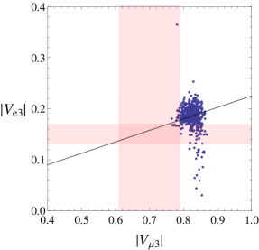
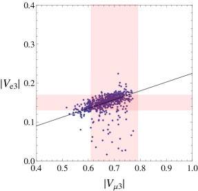
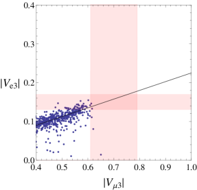
Combining these equations we obtain the relations linking PMNS and CKM mixing matrix elements:

$$V_{e3} \simeq -{V_{\mu 3}}{V_{us}}-\frac{V_{ub}}{\sqrt{2}}+{\cal O}(\epsilon),$$ (53)

$$V_{e2} \simeq \frac{1}{\sqrt{2}}\left(1-\frac{V_{ub}}{\sqrt{2}}\right)-V_{us}\left(1+\frac{V_{\mu 3}}{\sqrt{2}}\right)+{\cal O}(\epsilon).$$ (54)

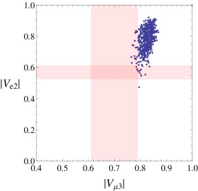
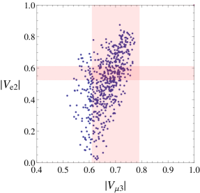
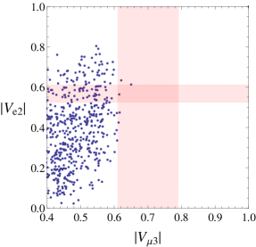
In order to check the robustness of these relations we perform a random scan of the free parameters in the Yukawa couplings, fixing only the absolute value of $|d|=1/7$ and allowing its phase and the rest of complex parameters of Eq. (40) $a,c,e,g$, to be random, with absolute values of ${\cal O}(1)$. The quark and charged lepton $c$-parameters are fixed to obtain good first order values of the CKM angles and of masses, whereas in the neutrino sector we take random values of $c_{\nu}^{1}$, $c_{\nu}^{2}$ and $c_{\nu}^{3}$, with the only constraint that the values are in the “neutrino plateau” (see Fig. 3) and that their values remain relatively degenerate. In particular we consider three windows, where we randomly scan, i.e., $c_{\nu}^{i}\in[-2.5,-2.3]$, $c_{\nu}^{i}\in[-2.2,-2.0]$ and $c_{\nu}^{i}\in[-2.0,-1.8]$. During the scan over random parameters, we keep only points that produce numerically correct CKM angles $|V_{us}|\simeq 0.22$, $|V_{cb}|\simeq 0.041$, and $|V_{ub}|\simeq 0.0035$, as well as correct neutrino mass differences. In Fig. 5, we test the correlation between $|V_{e3}|$ and $|V_{\mu 3}|$ and find it in very good agreement with Eq. (53). The bands in the graph represent the $3\sigma$ uncertainty around the central values obtained from experimental global fits Gonzalez-Garcia:2014bfa ; Maltoni:2004ei . It is quite remarkable that the theoretical correlation curve as well as most of the points generated for the intermediate window lie within these bounds. Higher values of $c_{\nu}^{i}$ and lower values of $c_{\nu}^{i}$ produce points with too high or too small $|V_{\mu 3}|$. Note that the lower values of $c_{\nu}^{i}$ lie at the end of the plateau and the beginning of the exponential sensitivity, and so these points start to show greater deviations from the expected correlation. For higher $c_{\nu}^{i}$ values however, the correlation is expected to be quite robust, although the experimental values might not agree with the obtained results.

Figure 6: Scan of the $V_{us}$ versus $V_{e3}$ with random perturbations around 2-3 symmetric Yukawa couplings as in the previous figures, with $c_{\nu}^{i}\in[-2.2,-2.0]$, and allowing for unphysical CKM entries (although still hierarchical), in order to test the quark lepton correlation expressed in Eq. (50) and shown in the graph with the diagonal line.

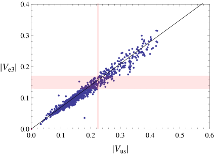
In order to further check this scenario, we perform the same scan as before but including all the points generated, without checking for correct CKM values (although in general they are quite CKM-like). This means that sometimes, the value of the Cabibbo angle is larger or smaller than expected due to accidental alignments or suppressions coming from the Yukawa couplings (taken randomly). Nevertheless the expectation is that the correlation between $V_{e3}$ and $V_{us}$ from Eq. (50) should survive, and indeed we see in Fig. 6 that this is the case. The exact values of the parameters used in the scan are obtained by adding small deviations to the zero-order values. In the case of the $c$-parameters we have thus $c_{f}^{i}=0.6\ \pm\ {\cal{O}}(0.1)$ for quarks and leptons, and $c_{\nu}^{i}=2\ \pm\ {\cal{O}}(0.1)$ for right-handed neutrinos. The Yukawa couplings are those given in Eq. (40), with the addition of small random perturbations.

IV Flavor democracy

In the second symmetry implementation, in this section we assume a democratic structure Harari:1978yi ; Pakvasa:1977in ; Pakvasa:1978tx ; Derman:1979nf ; Yamanaka:1981pa for all flavor parameters, meaning that in our case the 5D Yukawa couplings, $Y_{F}^{0}$ are invariant under $S_{3}\times S_{3}$ symmetry, while the 5D fermion bulk mass matrices, ${\mathbf{c}}^{0}_{f}$ are invariant under $S_{3}$ permutations. Explicitly, the democratic 5D Yukawa couplings and 5D fermion bulk mass matrices are given by

$$Y^{Dem}_{F}\propto\left(\begin{array}[]{ccc}1&1&1\\ 1&1&1\\ 1&1&1\end{array}\right)\ \ {\rm and}\ \ {\bf c}^{Dem}_{f}=\!\!\left(\begin{array}[]{ccc}a_{f}&b_{f}&b_{f}\\ b_{f}&a_{f}&b_{f}\\ b_{f}&b_{f}&a_{f}\end{array}\right)\,.\ \ \$$ (61)

Overall, there are four Yukawa matrices, $Y^{Dem}_{u}$, $Y^{Dem}_{d}$, $Y^{Dem}_{e}$ and $Y^{Dem}_{\nu}$, corresponding to the up-quark sector, the down-quark sector, the charged leptons and the neutrinos. There are six fermion bulk $c$-matrices, namely ${\bf c}^{Dem}_{q}$, ${\bf c}^{Dem}_{u}$, ${\bf c}^{Dem}_{d}$, ${\bf c}^{Dem}_{l}$, ${\bf c}^{Dem}_{e}$ and ${\bf c}^{Dem}_{\nu}$.

Both matrices can be simultaneously diagonalized by the same unitary transformation resulting in two zero eigenvalues for the Yukawa matrices, and two degenerate eigenvalues for the bulk mass matrices, ${\mathbf{c}}_{f}^{Dem}$. The 5D Yukawa and bulk mass matrices thus become, in their diagonal basis

$$Y^{0}_{F}=y^{0}_{{}_{F}}\left(\begin{array}[]{ccc}0&0&0\\ 0&0&0\\ 0&0&1\end{array}\right)\ {\rm and}\ \ {\bf c}^{0}_{f}=\!\!\left(\begin{array}[]{ccc}c^{1^{0}}_{f}&0&0\\ 0&c^{1^{0}}_{f}&0\\ 0&0&c^{3^{0}}_{f}\end{array}\right),\ \ \ \ \ \$$ (68)

where $y_{F}^{0}$ are complex Yukawa couplings and the index $F$ runs over $u$, $d$, $e$, and $\nu$. The elements $c^{i\,0}_{f}$ are real and the index $f_{i}$ runs over doublets $q_{i}$, $l_{i}$ as well as singlets $u_{i}$, $d_{i}$, $\nu_{i}$ and $e_{i}$, with $i$ the flavor index. Note that in this flavor symmetric limit, all fermions except the $t$ quark, $b$ quark, $\tau$ lepton and $\nu_{\tau}$ neutrino, are massless. The 5D flavor structure of Eq. (68) yields the 0-th order CKM and PMNS matrices for this scenario

$$V^{0}_{i}\!=\left(\begin{array}[]{ccc}\vphantom{\frac{9}{\sqrt{3}}}\cos{\theta^{0}_{i}}&\sin{\theta^{0}_{i}}&\ 0\\ \vphantom{\frac{\sqrt{9}}{\sqrt{3}}}-\sin{\theta^{0}_{i}}&\cos{\theta^{0}_{i}}&\ 0\\ \vphantom{\frac{9}{\sqrt{3}}}0&0&\ 1\end{array}\right)\,,\ \$$ (72)

where $i=$CKM, PMNS. The angle $\theta_{i}^{0}$, depends on the detailed structure of the symmetry breaking terms, $\delta Y_{F}$ and ${\delta\mathbf{c}}_{f}$ in Eqs. (23) and (22), and is not fixed by the underlying $S_{3}\times S_{3}$ symmetry. Addition of generic small perturbations, as in Eqs. (22) and (23), breaks the flavor symmetry and lifts the degeneracies to produce SM-like masses and mixing angles. In the neutrino sector, the two level degeneracy is lifted by a small amount $(\delta Y_{F})_{ij}$. This suggests a normal hierarchy ordering with one heavier eigenstate, and with two lighter ones having similar masses. Using Eq. (II) and taking the generic size of the perturbations as $(\delta Y_{F})_{ij}\simeq\delta Y^{\nu}$ for simplicity, yields the following relations for the neutrino masses

$$m_{1} \sim\delta Y^{\nu}\ v\ e^{-ky_{1}(a-1)}\ ,\qquad m_{2}\sim\delta Y^{\nu}\ v\ e^{-ky_{1}(a-1)}\ ,\qquad m_{3} \sim(1+\delta Y^{\nu})v\ e^{-ky_{1}(a-1)}.$$ (73)

Neutrino mass data requires $v\ e^{-ky_{1}(a-1)}\simeq 0.3$ eV and

explaining the hierarchy problem requires $ky_{1}\simeq 35$, which means that the value of the Higgs localization parameter should be about $a\simeq 1.8$. As explained in a previous section, this value of $a$ requires some fine-tuning of parameters in the RS 5D Higgs potential. With modified $AdS_{5}$ metrics it is possible to remain in a non-tuned region, and in particular we find that the best region is obtained for $\nu\sim 0.2$ and $kL_{1}\sim 0.3$, where the parameter $a$ can have values as large as $4.5$. In order to obtain the observed neutrino mass hierarchy ratio $r$, defined as $r=(|m_{2}|^{2}-|m_{1}|^{2})/(|m_{3}|^{2}-|m_{1}|^{2})\simeq 0.03$, the size of the Yukawa coupling perturbations $\delta Y$ must be fixed to $\delta Y^{\nu}\mathrel{\raise 1.29167pt\hbox{$<$\kern-7.5pt\lower 4.30554pt\hbox{$\sim$}}}\sqrt{r}\simeq 0.17$. There are no restrictions on the values of bulk mass parameters $c_{\psi}^{i}$-s (as long as they are within the bounds $a<c_{\nu}+c_{l}$).

Consider the elements $V_{e2}$, $V_{e3}$ and $V_{\mu 3}$ of the PMNS matrix. As mentioned before, due to the plateau in the neutrino sector, for a small $a$ parameter, the 5D Yukawa matrix structure is more or less preserved and therefore these elements should be close to the ones shown in Eq. (72) plus some perturbations. This matrix predicts very small values for both $|V_{e3}|$ and $|V_{\mu 3}|$ and so the perturbations should lift them (especially $|V_{\mu 3}|$). The value of $V_{e2}$ on the other hand is highly sensitive to the structure of the neutrino Yukawa flavor violating matrix $\delta Y^{\nu}_{ij}$ and can be large or small.

Figure 7: Scatter plots of $V_{e3}$ versus $V_{\mu 3}$ with random values of $\delta Y_{\nu}$, $\delta Y_{e}$, $c_{l}$ and $c_{\nu}$. We have fixed $c_{l}^{3}=0.41$ and $(\delta Y^{\nu})_{23}=0.13$ and then taken $(\delta Y^{\nu})_{13}=0.002$ (left panel) $(\delta Y^{\nu})_{13}=0.008$ (central panel) and $(\delta Y^{\nu})_{13}=0.032$ (right panel). The concentration of points in a precise region shows that the mixing angles $V_{e3}$ and $V_{\mu 3}$ are sensitive to only these three parameters. The obtained values of $V_{\mu 3}$ lie on the lower side of the experimental window, whereas $V_{e3}$ depends on the ratio of Yukawa couplings $(\delta Y^{\nu})_{13}/(\delta Y^{\nu})_{23}$, so that its smallness is due to a slight hierarchy in these.

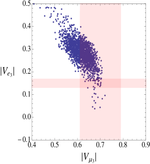
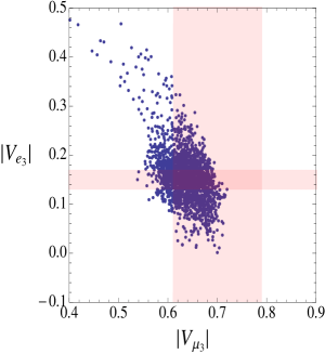
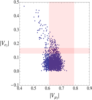
It turns out that when the c-parameters are such that, $a<c_{l}^{3}+c_{\nu}^{j}$ and $c_{l}^{3}<1/2$ (a region not generic in usual warped extra dimension scenarios) the lifting of the zero-order PMNS can be successful and we have

$$V_{e2}\sim\sin{\theta}^{0}_{\nu}\ ,$$ (74)

$$V_{e3}\propto\delta Y^{\nu}_{13}\ f(c^{3}_{l})\ ,$$ (75)

$$V_{\mu 3}\propto\delta Y^{\nu}_{23}\ f(c^{3}_{l})\ .\ \ \$$ (76)

Note in particular that we expect that $V_{e3}/V_{\mu 3}\propto\delta Y^{\nu}_{13}/\delta Y^{\nu}_{23}$. In Fig. 7 we present a scan of the model parameters to verify the validity of Eq. (74). In this scan we randomly perturbed the values of the 5D parameters $Y_{\nu}$, $Y_{e}$, $c_{l}$ and $c_{\nu}$, but kept the values of the three relevant parameters $c^{3}_{l}$, $\delta Y^{\nu}_{13}$ and $\delta Y^{\nu}_{23}$ fixed. We see from the figure that the values obtained for the matrix elements $V_{\mu 3}$ and $V_{e3}$ can be made to lie within the experimental bounds by fixing only these three parameters with all other terms randomly perturbed. In particular, the formulas show the sensitivity of these two PMNS mixing angles to the flavor structure of the neutrino Yukawa matrix $\delta Y^{\nu}$, but not to the charged lepton Yukawa matrix $\delta Y^{l}$ or to the bulk masses $\delta c_{\psi}^{i}$, except for $\delta c^{3}_{l}$. Knowing that experimentally $V_{\mu 3}^{\rm exp}\simeq 0.65$ and $V_{e3}^{\rm exp}\simeq 0.15$, for the numerical evaluations we took the bulk mass parameter of the third family lepton doublet $c^{3}_{l}<1/2$ to obtain larger mixing angles for small $\delta Y\simeq 0.1$, the same as in the quark sector, where $c^{3}_{q}\lesssim 1/2$ is needed to obtain a large top quark mass, and thus it could be a hinting of a possible additional family symmetry among the $SU(2)$ doublets of the third family. The particular values used in the scan are $c_{l}^{3}=0.41$, $\delta Y^{\nu}_{13}=0.008$ and $\delta Y^{\nu}_{23}=0.13$, which produce PMNS angles consistent with experiment but with $|V_{\mu 3}|$ on the lower experimental side. When the experimental uncertainty decreases and if the central value of $|V_{\mu 3}^{\rm exp}|$ ends up in the higher end of the current allowed region, this scenario will be under great pressure. We also show how indeed the ratio $V_{e3}/V_{\mu 3}$ depends on the ratio $\delta Y^{\nu}_{13}/\delta Y^{\nu}_{23}$ by increasing and decreasing the value of $\delta Y^{\nu}_{13}$ resulting in larger or smaller values of $|V_{e3}|$.

In the charged lepton sector and the up- and down-quark sectors, massless states are also lifted by the flavor symmetry breaking, and these masses emerge directly proportional to the generic size of the perturbations in the Yukawa matrix, $\delta Y$, as described in Frank:2014aca .

Finally, in Table 1 we present a set of $S_{3}$ symmetric 0-th order bulk c-parameters (many other points with the same symmetry in the parameter space are possible), which, with a small perturbation of order $\delta c\simeq\delta Y\simeq 10\%$, can lead to the SM in the modified $AdS_{5}$ scenario. For this specific point we have taken the value of the warp exponent at the IR brane, $A(y_{1})$ to be exactly 35. With this assignment, there is only one more free parameter in the model left to completely fix the metric. This parameter can be either $\nu$, or the position of the singularity, $y_{s}$. Therefore one has the freedom to choose the amount of departure from the pure $AdS_{5}$. For the point presented in Table 1, we took $\nu\simeq 0.32$ and the value of the localization of the Higgs field operator $a$ is $4.46$ as in the previous example. With this starting point, the SM is then easily reproduced by breaking the symmetry through adding perturbations $\delta c^{i}$-s and $\delta Y_{ij}$-s to lift the degeneracies of the symmetric scenario. We require $\delta Y_{ij}\lesssim 0.1$ and $\delta c_{\psi}^{i}\lesssim 0.1$ parameters to produce the SM masses, angles and phases, by systematically using the approximate formulas in this section up to any order of precision consistent with the SM. In general the sensitivity to the precise values of the 5D Yukawa couplings, $\delta Y_{ij}$, is minimal and randomly chosen matrices with $\delta Y_{ij}\lesssim 0.1$ produce all the required SM features.

$f$	$q$	$l$	$u$	$d$	$e$	$\nu$
$c^{1^{0}}_{f}$	0.55	0.55	0.55	0.65	0.65	5.00
$c^{3^{0}}_{f}$	0.45	0.45	0.45	0.65	0.65	3.00

Table 1: A parameter point for democratic flavor symmetry in the localization parameters space (out of many possible points) in the 0-th order 5D fermion $c$-parameter space, consistent with all the experimental and model constraints. For this point, we have set all the 0-th order Yukawa coefficients to be universal, $y^{0}_{u}=y^{0}_{d}=y^{0}_{\nu}=y^{0}_{e}=4.4$, and the Higgs localization parameter to $a=2.1$. The modified $AdS_{5}$ metric parameters are $\nu=1.1$, $y_{1}=2.8\times 10^{-17}$, and $A(y_{1})=35$.

V Conclusion

In this work, we have provided a warped extra dimensional framework in which all of the fermions, including neutrinos, are treated on equal footing, and where the SM fermion flavor structure can still emerge naturally out of a slightly broken universal flavor symmetry. Essential for this scenario is that all the matter fields must be in the bulk and, in particular the Higgs field should be as delocalized as possible from the IR boundary. We have explored a general warped scenario in which the metric is modified from the usual $AdS_{5}$ background. This setup has the advantage of allowing lower KK masses ($\sim$ 1-2 TeV), while still safe from precision electroweak tests and flavor bounds. For our study, the modified metric presents a further advantage, as the neutrino mass generation in our framework is more natural. This is due to a numerical accident by which the neutrino masses generated in the $AdS_{5}$ background are too small (at most $\sim 10^{-4}$ eV) in the parameter region of interest (neutrino plateau), while in the modified metric neutrino masses can be up to two orders of magnitude larger, in the same qualitative region of parameter space. A way out in $AdS_{5}$ would be to further delocalize the Higgs field, although requiring such a delocalized Higgs to generically solve the hierarchy problem, some degree of fine-tuning must be introduced in the Higgs potential. These tensions disappear when we use a modified $AdS_{5}$ geometry, where our flavor setup can be successfully implemented without further fine-tuning.

In the parameter region of interest (the neutrino plateau) the effective 4D neutrino masses do not have exponential dependence on the bulk mass parameters $c^{i}$, in contrast with quark and charged lepton masses. Once a universal flavor symmetry is slightly broken, the SM flavor structure emerges due to the inherent features of warped space models, i.e. the wave function profiles of light quarks and charged leptons are exponentially sensitive to the symmetry violating terms, resulting in masses and mixing controlled by small flavor violating terms. In the neutrino sector, in the plateau region with a highly delocalized Higgs field, the wave functions are not exponentially sensitive to Lagrangian parameters and thus the original flavor symmetry is essentially preserved. Overall results are similar in both RS and modified $AdS_{5}$ type of scenarios, indicating that the precise nature of the flavor symmetry or the precise nature of the metric solution is not crucial for the main property of the scenarios.

For illustration, we chose two simple examples of different symmetries which can provide an implementation for this mechanism. In the first scenario, we study quark lepton complementarity associated with $\mu-\tau$ symmetry (or 2-3 symmetry), known to lead to phenomenologically viable neutrino masses and mixings. Assuming equal Yukawa matrix couplings in the charged lepton and down-quark sector, and equal Yukawa matrix couplings in the neutrino and up quark sector, as well as identical localization for the doublet quark and lepton representations, mass differences emerge entirely from singlet representation localization. The predictions of this implementation are definite connections between PMNS and CKM matrix elements, as given by Eqs. (53) and (54).

In the second example, flavor democracy, the 5D Yukawa couplings for the fermions are invariant under the $S_{3}\times S_{3}$ symmetry, while the 5D fermion bulk mass matrices are invariant under $S_{3}$ family permutation invariance. Small perturbations of ${\cal O}(10\%)$ are enough to generate the full flavor structure of the SM in both quark and lepton sectors, and the ratio of PMNS matrix elements can be simply expressed in terms of these perturbations. Explicit expressions appear in Eqs. (74). Localization of the third lepton family follows localization of the third quark family, hinting at an additional quark-lepton symmetry. As distinctive predictions and correlations appear in each implementation, the model studied here would yield a very promising novel laboratory for studying fermion flavor symmetries.

VI Appendix: Explicit expressions for the field profiles

Here we derive the explicit expressions for the fermion and Higgs profiles, as well as for the Yukawa couplings for the modified $AdS_{5}$ scenario. The fermion profiles are given by

$$q^{0,i}_{L}(y)=q^{i}_{0}e^{(2-c_{q}^{i})A(y)}\ ,\qquad u^{0,i}_{R}=u^{i}_{0}e^{(c_{u}^{i}+2)A(y)}\ ,$$ (77)

while the Higgs profile is

$$h(y)=h_{0}e^{aky}\ ,$$ (78)

with

$$q^{i}_{0}=\sqrt{k}\epsilon^{{1\over 2}-c_{q}^{i}}f(c_{q}^{i})\equiv\sqrt{k}\mathfrak{f}(c_{q}^{i})\ ,\qquad u^{i}_{0}=\sqrt{k}\epsilon^{{1\over 2}+c_{u}^{i}}f(-c_{u}^{i})\equiv\sqrt{k}\mathfrak{f}(-c_{u}^{i})\ ,$$ (79)

and

$$h_{0} \equiv \sqrt{k}e^{-(a-1)ky_{s}}\mathfrak{h}_{0}$$ (80)

$$\!\!\mathfrak{h}_{0} = \frac{1}{\sqrt{ky_{s}(2(a-1)ky_{s})^{-\frac{2}{\nu^{2}}-1}\left(\Gamma\left(1+\frac{2}{\nu^{2}},2(a-1)k(y_{s}-y_{1})\right)-\Gamma\left(1+\frac{2}{\nu^{2}},2(a-1)ky_{s}\right)\right)}},$$

where

$$\epsilon=e^{-A(y)}=e^{-ky_{1}}\left(1-\frac{y_{1}}{y_{s}}\right)^{\frac{1}{\nu^{2}}}\ .$$ (81)

The reduced profile functions $\mathfrak{f}(c)$ are defined as   $\mathfrak{f}(c)\equiv\epsilon^{{1\over 2}-c}f(c)\ ,\quad{\text{with}}$

$$f(c)\equiv$$ (82)

$$\!\!\frac{\epsilon^{c-{1\over 2}}}{\sqrt{ky_{s}e^{(1-2c)ky_{s}}((1\!-\!2c)ky_{s})^{\frac{1\!-\!2c}{\nu^{2}}-1}\left(\Gamma\left(1-\frac{1\!-\!2c}{\nu^{2}},(1\!-\!2c)k(y_{s}-y_{1})\right)\!-\!\Gamma\left(1-\frac{1\!-\!2c}{\nu^{2}},(1\!-\!2c)ky_{s}\right)\right)}}.$$

Note that the Higgs and the fermion profiles are defined differently, due to the specific Higgs potential we have considered Azatov:2009na . We can now write down the most general form for the Yukawa couplings as

$$y_{ij}^{u}=\tilde{Y}^{u}_{ij}h_{0}f(c_{q}^{i})f(-c_{u}^{j})\ ,$$ (83)

where the $\tilde{Y}_{ij}$s are related to the 5D Yukawa couplings via the equation

$$\tilde{Y}_{ij}^{u} \equiv Y_{ij}^{u}\sqrt{k}\epsilon^{1-c_{q}+c_{u}}y_{s}e^{ky_{s}(a-c_{q}^{i}+c_{u}^{j})}\left[ky_{s}(a-c_{q}^{i}+c_{u}^{j})\right]^{\frac{c_{u}^{j}-c_{q}^{i}}{\nu^{2}}-1}$$

$$\left[\Gamma\left(\frac{c_{q}^{i}-c_{u}^{j}}{\nu^{2}}+1,(a-c_{q}^{i}+c_{u}^{j})k(y_{s}-y_{1})\right)-\Gamma\left(\frac{c_{q}^{i}-c_{u}^{j}}{\nu^{2}}+1,(a-c_{q}^{i}+c_{u}^{j})ky_{s}\right)\right]\ .$$

Before switching to the expressions in the RS metric, we use the asymptotic expansion of the incomplete Gamma function

$$\Gamma\!\left(a,z\right)\sim z^{a-1}e^{-z}\left(1+{a-1\over z}+{(a-1)(a-2)\over z^{2}}+\mathcal{O}(z^{-3})\right)\,.$$ (85)

Then we get the following asymptotic behavior, up to the first order in $\mathcal{O}(z^{a-1})$, with $\epsilon$ defined as in Eq. (81)

$$f(c) \sim \sqrt{{1-2c\over 1-\epsilon^{1-2c}}}\ ,$$ (86)

$$h_{0} \sim \sqrt{2(1-a)\over 1-e^{2aky_{1}}\epsilon^{2}}\ ,$$ (87)

$$\tilde{Y}_{ij}^{u} \sim \frac{e^{aky_{1}}\epsilon^{c^{i}_{q}-c^{j}_{u}}-1}{a-c_{q}^{i}+c_{u}^{j}}Y_{ij}^{u}\ .$$ (88)

Keeping the $\mathcal{O}(z^{a-2})$ term not only gives a much better approximation for the top and neutrino plateaux, but it also gives a more transparent expression for these functions:

$$f(c) \sim \epsilon^{c-{1\over 2}}\sqrt{{(1-2c)ky_{s}\nu^{2}\over ky_{s}\nu^{2}(\epsilon^{2c-1}-1)-\epsilon^{2c-1}+\left({y_{s}\over y_{s}-y_{1}}\right)}}\ ,$$ (89)

$$h_{0} \sim \epsilon^{-1}e^{-aky_{1}}\sqrt{{2(1-a)^{2}\ ky_{s}\nu^{2}\over ky_{s}\nu^{2}(1-a)(\epsilon^{-2}e^{-2aky_{1}}-1)-\epsilon^{-2}e^{-2aky_{1}}+\left({y_{s}\over y_{s}-y_{1}}\right)}}\ .$$ (90)

From these formulas, valid for the general modified $AdS_{5}$ metric, one can see that, taking the limits $\nu\rightarrow\infty$ and $y_{s}\rightarrow\infty$ we obtain the expressions for the profiles in the RS metric:

$$f^{RS}(c) = \sqrt{{1-2c\over 1-\epsilon^{1-2c}}}\equiv\epsilon^{c-{1\over 2}}\mathfrak{f}^{RS}(c)\ ,\qquad h_{0}^{RS}=e^{(1-a)ky_{1}}\sqrt{2(1-a)\over\epsilon^{2(a-1)}-1}\ ,$$ (91)

$$\tilde{Y}_{ij}^{RS,u} \equiv \frac{\epsilon^{-(a-c_{q}^{i}+c_{u}^{j})}-1}{a-c_{q}^{i}+c_{u}^{j}}Y_{ij}^{RS,u}\ ,\qquad y_{ij}^{RS,u}=\tilde{Y}_{ij}^{RS,u}h_{0}^{RS}f^{RS}(c_{q}^{i})f^{RS}(-c_{u}^{j})\ .$$ (92)

where $\epsilon\equiv e^{-ky_{1}}$.

References

- (1) F. P. An et al. [DAYA-BAY Collaboration], Phys. Rev. Lett. 108, 171803 (2012).
- (2) F. P. An et al. [Daya Bay Collaboration], Chin. Phys. C 37, 011001 (2013).
- (3) K. Abe et al. [T2K Collaboration], Phys. Rev. Lett. 107, 041801 (2011).
- (4) K. Abe et al. [T2K Collaboration], Phys. Rev. Lett. 112, no. 18, 181801 (2014).
- (5) P. Adamson et al. [MINOS Collaboration], Phys. Rev. Lett. 106, 181801 (2011).
- (6) P. Adamson et al. [MINOS Collaboration], Phys. Rev. Lett. 112, 191801 (2014).
- (7) J. K. Ahn et al. [RENO Collaboration], Phys. Rev. Lett. 108, 191802 (2012).
- (8) Y. Abe et al. [Double Chooz Collaboration], Phys. Rev. D 86, 052008 (2012)
- (9) Y. Abe et al. [Double Chooz Collaboration], JHEP 1410, 86 (2014).
- (10) P. Minkowski, Phys. Lett. B 67, 421 (1977).
- (11) M. Gell-Mann, P. Ramond, and R. Slansky, in “Supergravity”, ed. P. van Niewenhuizen and D. Freedman (North Holland, Amsterdam, 1980), p. 315.
- (12) T. Yanagida, ed., Proceedings of the Workshop on the Unified Theory and the Baryon Number in the Universe, edited by O. Sawada and A. Sugamoto (KEK, Tsukuba, Japan, 1979) p. 95.
- (13) S. L. Glashow, in Proceedings of the 1979 Cargese Summer Institute on Quarks and Leptons, edited by M. Levy et al. (Plenum Press, New York, 1980), p. 687.
- (14) R. N. Mohapatra and G. Senjanovic, Phys. Rev. Lett. 44, 912 (1980).
- (15) J. Schechter and J. W. F. Valle, Phys. Rev. D 22, 2227 (1980).
- (16) G. Lazarides, Q. Shafi and C. Wetterich, Nucl. Phys. B 181, 287 (1981).
- (17) P. H. Frampton, S. L. Glashow and D. Marfatia, Phys. Lett. B 536, 79 (2002).
- (18) L. Lavoura, Phys. Lett. B 609, 317 (2005).
- (19) S. Dev, S. Verma, S. Gupta and R. R. Gautam, Phys. Rev. D 81, 053010 (2010).
- (20) C. S. Lam, Phys. Rev. Lett. 101, 121602 (2008).
- (21) C. S. Lam, Phys. Rev. D 78, 073015 (2008).
- (22) W. Grimus, L. Lavoura and P. O. Ludl, J. Phys. G 36, 115007 (2009).
- (23) S. F. Ge, D. A. Dicus and W. W. Repko, Phys. Lett. B 702, 220 (2011).
- (24) H. J. He and F. R. Yin, Phys. Rev. D 84, 033009 (2011).
- (25) R. d. A. Toorop, F. Feruglio and C. Hagedorn, Phys. Lett. B 703, 447 (2011).
- (26) S. F. Ge, D. A. Dicus and W. W. Repko, Phys. Rev. Lett. 108, 041801 (2012).
- (27) R. de Adelhart Toorop, F. Feruglio and C. Hagedorn, Nucl. Phys. B 858, 437 (2012).
- (28) H. J. He and X. J. Xu, Phys. Rev. D 86, 111301 (2012).
- (29) D. Hernandez and A. Y. Smirnov, Phys. Rev. D 86, 053014 (2012).
- (30) C. S. Lam, Phys. Rev. D 87, 013001 (2013).
- (31) D. Hernandez and A. Y. Smirnov, Phys. Rev. D 87, no. 5, 053005 (2013).
- (32) M. Holthausen, K. S. Lim and M. Lindner, Phys. Lett. B 721, 61 (2013).
- (33) B. Hu, Phys. Rev. D 87, no. 3, 033002 (2013).
- (34) D. Hernandez and A. Y. Smirnov, Phys. Rev. D 88, no. 9, 093007 (2013).
- (35) S. F. King, T. Neder and A. J. Stuart, Phys. Lett. B 726, 312 (2013).
- (36) C. Hagedorn, A. Meroni and L. Vitale, J. Phys. A 47, 055201 (2014).
- (37) L. Lavoura and P. O. Ludl, Phys. Lett. B 731, 331 (2014).
- (38) P. F. Harrison, D. H. Perkins and W. G. Scott, Phys. Lett. B 458, 79 (1999).
- (39) P. F. Harrison, D. H. Perkins and W. G. Scott, Phys. Lett. B 530, 167 (2002).
- (40) Z. z. Xing, Phys. Lett. B 533, 85 (2002).
- (41) P. F. Harrison and W. G. Scott, Phys. Lett. B 535, 163 (2002).
- (42) P. F. Harrison and W. G. Scott, Phys. Lett. B 557, 76 (2003).
- (43) X. G. He and A. Zee, Phys. Lett. B 560, 87 (2003).
- (44) F. Vissani, hep-ph/9708483.
- (45) V. D. Barger, S. Pakvasa, T. J. Weiler and K. Whisnant, Phys. Lett. B 437, 107 (1998).
- (46) A. J. Baltz, A. S. Goldhaber and M. Goldhaber, Phys. Rev. Lett. 81, 5730 (1998).
- (47) I. Stancu, D. V. Ahluwalia and , Phys. Lett. B 460, 431 (1999).
- (48) H. Georgi and S. L. Glashow, Phys. Rev. D 61, 097301 (2000).
- (49) N. Li and B. Q. Ma, Phys. Lett. B 600, 248 (2004).
- (50) H. Fritzsch and Z. Z. Xing, Phys. Lett. B 372, 265 (1996).
- (51) H. Fritzsch and Z. z. Xing, Phys. Lett. B 440, 313 (1998).
- (52) H. Fritzsch and Z. z. Xing, Phys. Rev. D 61, 073016 (2000).
- (53) Y. Zhang, X. Zhang and B. Q. Ma, Phys. Rev. D 86, 093019 (2012).
- (54) X. Zhang, Y. j. Zheng and B. Q. Ma, Phys. Rev. D 85, 097301 (2012).
- (55) G. N. Li, H. H. Lin and X. G. He, Phys. Lett. B 711, 57 (2012).
- (56) S. K. Kang, Phys. Rev. D 83, 097301 (2011).
- (57) Y. H. Ahn, H. Y. Cheng and S. Oh, Phys. Rev. D 83, 076012 (2011).
- (58) Y. Shimizu and R. Takahashi, Europhys. Lett. 93, 61001 (2011).
- (59) K. M. Patel, Phys. Lett. B 695, 225 (2011).
- (60) J. Barranco, F. Gonzalez Canales and A. Mondragon, Phys. Rev. D 82, 073010 (2010).
- (61) Y. j. Zheng, Phys. Rev. D 81, 073009 (2010).
- (62) Z. z. Xing, Phys. Lett. B 679, 111 (2009).
- (63) P. H. Frampton and S. Matsuzaki, Mod. Phys. Lett. A 24, 429 (2009).
- (64) W. Rodejohann and K. A. Hochmuth, Int. J. Mod. Phys. A 22, 5875 (2007).
- (65) F. Plentinger, G. Seidl and W. Winter, Phys. Rev. D 76, 113003 (2007).
- (66) M. Picariello, B. C. Chauhan, J. Pulido and E. Torrente-Lujan, Int. J. Mod. Phys. A 22, 5860 (2007).
- (67) L. Randall and R. Sundrum, Phys. Rev. Lett. 83, 3370 (1999).
- (68) L. Randall and R. Sundrum, Phys. Rev. Lett. 83, 4690 (1999).
- (69) Y. Grossman and M. Neubert, Phys. Lett. B 474, 361 (2000).
- (70) T. Gherghetta and A. Pomarol, Nucl. Phys. B 586, 141 (2000).
- (71) H. Davoudiasl, J. L. Hewett and T. G. Rizzo, Phys. Lett. B 473, 43 (2000).
- (72) S. Chang, J. Hisano, H. Nakano, N. Okada and M. Yamaguchi, Phys. Rev. D 62, 084025 (2000).
- (73) S. J. Huber, Nucl. Phys. B 666, 269 (2003).
- (74) S. Casagrande, F. Goertz, U. Haisch, M. Neubert and T. Pfoh, JHEP 1009, 014 (2010).
- (75) K. Agashe, G. Perez and A. Soni, Phys. Rev. D 71, 016002 (2005).
- (76) K. Agashe, A. Delgado, M. J. May and R. Sundrum, JHEP 0308 (2003) 050.
- (77) G. Burdman, Phys. Rev. D 66, 076003 (2002).
- (78) G. Burdman, Phys. Lett. B 590, 86 (2004).
- (79) M. S. Carena, A. Delgado, E. Ponton, T. M. P. Tait and C. E. M. Wagner, Phys. Rev. D 71, 015010 (2005).
- (80) M. S. Carena, A. Delgado, E. Ponton, T. M. P. Tait and C. E. M. Wagner, Phys. Rev. D 68, 035010 (2003).
- (81) A. Delgado and A. Falkowski, JHEP 0705, 097 (2007).
- (82) M. Quiros, arXiv:1311.2824 [hep-ph].
- (83) C. Csaki, A. Falkowski and A. Weiler, JHEP 0809, 008 (2008).
- (84) K. Agashe, A. Azatov and L. Zhu, Phys. Rev. D 79, 056006 (2009).
- (85) K. Agashe, R. Contino, L. Da Rold and A. Pomarol, Phys. Lett. B 641, 62 (2006).
- (86) A. Falkowski and M. Perez-Victoria, JHEP 0812, 107 (2008).
- (87) B. Batell, T. Gherghetta and D. Sword, Phys. Rev. D 78, 116011 (2008).
- (88) S. Mert Aybat and J. Santiago, Phys. Rev. D 80, 035005 (2009).
- (89) J. A. Cabrer, G. von Gersdorff and M. Quiros, New J. Phys. 12, 075012 (2010).
- (90) J. A. Cabrer, G. von Gersdorff and M. Quiros, Phys. Lett. B 697, 208 (2011).
- (91) J. A. Cabrer, G. von Gersdorff and M. Quiros, JHEP 1105, 083 (2011).
- (92) A. Azatov, M. Toharia and L. Zhu, Phys. Rev. D 82, 056004 (2010).
- (93) M. Frank, N. Pourtolami and M. Toharia, Phys. Rev. D 87, 096003 (2013).
- (94) M. Frank, N. Pourtolami and M. Toharia, Phys. Rev. D 89, 016012 (2014).
- (95) C. Csaki, C. Delaunay, C. Grojean and Y. Grossman, JHEP 0810, 055 (2008).
- (96) K. Agashe, T. Okui and R. Sundrum, Phys. Rev. Lett. 102, 101801 (2009).
- (97) M. Frank, C. Hamzaoui, N. Pourtolami and M. Toharia, Phys. Lett. B 742, 178 (2015).
- (98) A. Carmona and J. Santiago, JHEP 1201, 100 (2012).
- (99) J. A. Cabrer, G. von Gersdorff and M. Quiros, JHEP 1201, 033 (2012).
- (100) J. de Blas, A. Delgado, B. Ostdiek and A. de la Puente, Phys. Rev. D 86, 015028 (2012).
- (101) K. A. Olive et al. [Particle Data Group Collaboration], Chin. Phys. C 38, 090001 (2014).
- (102) S. Casagrande, F. Goertz, U. Haisch, M. Neubert and T. Pfoh, JHEP 0810, 094 (2008).
- (103) H. Harari, H. Haut and J. Weyers, Phys. Lett. B 78, 459 (1978).
- (104) S. Pakvasa and H. Sugawara, Phys. Lett. B 73, 61 (1978).
- (105) S. Pakvasa and H. Sugawara, Phys. Lett. B 82, 105 (1979).
- (106) E. Derman and H. S. Tsao, Phys. Rev. D 20, 1207 (1979).
- (107) Y. Yamanaka, H. Sugawara and S. Pakvasa, Phys. Rev. D 25, 1895 (1982) [Erratum-ibid. D 29, 2135 (1984)].
- (108) E. Ma and M. Raidal, Phys. Rev. Lett. 87, 011802 (2001) [Erratum-ibid. 87, 159901 (2001)].
- (109) W. Grimus and L. Lavoura, JHEP 0107, 045 (2001)
- (110) R. N. Mohapatra and S. Nasri, Phys. Rev. D 71, 033001 (2005).
- (111) R. N. Mohapatra, S. Nasri and H. B. Yu, Phys. Lett. B 615, 231 (2005).
- (112) S. Nasri, Int. J. Mod. Phys. A 20, 6258 (2005).
- (113) R. N. Mohapatra, S. Nasri and H. B. Yu, Phys. Lett. B 636, 114 (2006).
- (114) R. N. Mohapatra, S. Nasri and H. B. Yu, Phys. Lett. B 639, 318 (2006).
- (115) Z. z. Xing, H. Zhang and S. Zhou, Phys. Lett. B 641, 189 (2006).
- (116) Y. H. Ahn, S. K. Kang, C. S. Kim and J. Lee, Phys. Rev. D 73, 093005 (2006).
- (117) I. Aizawa and M. Yasue, Phys. Rev. D 73, 015002 (2006).
- (118) K. Fuki and M. Yasue, Phys. Rev. D 73, 055014 (2006). [hep-ph/0601118].
- (119) A. S. Joshipura, Eur. Phys. J. C 53, 77 (2008).
- (120) B. Adhikary, A. Ghosal and P. Roy, JHEP 0910, 040 (2009).
- (121) Z. z. Xing and Y. L. Zhou, Phys. Lett. B 693, 584 (2010).
- (122) S. F. Ge, H. J. He and F. R. Yin, JCAP 1005, 017 (2010).
- (123) I. de Medeiros Varzielas, R. Gonzalez Felipe and H. Serodio, Phys. Rev. D 83, 033007 (2011).
- (124) S. Gupta, A. S. Joshipura and K. M. Patel, JHEP 1309, 035 (2013).
- (125) B. Adhikary, M. Chakraborty and A. Ghosal, JHEP 1310, 043 (2013) [Erratum-ibid. 1409, 180 (2014)].
- (126) B. Adhikary, A. Ghosal and P. Roy, Int. J. Mod. Phys. A 28, no. 24, 1350118 (2013).
- (127) J. Liao, D. Marfatia and K. Whisnant, Phys. Rev. D 87, 013003 (2013).
- (128) C. Hamzaoui, S. Nasri and M. Toharia, Phys. Rev. D 89, no. 7, 073019 (2014).
- (129) E. I. Lashin, N. Chamoun, C. Hamzaoui and S. Nasri, Phys. Rev. D 89, no. 9, 093004 (2014).
- (130) M. C. Gonzalez-Garcia, M. Maltoni and T. Schwetz, JHEP 1411, 052 (2014).
- (131) M. Maltoni, T. Schwetz, M. A. Tortola and J. W. F. Valle, New J. Phys. 6, 122 (2004)
- (132) A. Azatov, M. Toharia and L. Zhu, Phys. Rev. D 80, 035016 (2009).