Accurate and Approximate Calculations of Raman Scattering in the Atmosphere of Neptune
Abstract
Raman scattering by H2 in Neptune’s atmosphere has significant effects on its reflectivity for 0.5 m, producing baseline decreases of 20% in a clear atmosphere and 10% in a hazy atmosphere. However, few accurate Raman calculations are carried out because of their complexity and computational costs. Here we present the first radiation transfer algorithm that includes both polarization and Raman scattering and facilitates computation of spatially resolved spectra. New calculations show that Cochran and Trafton’s (1978, Astrophys. J. 219, 756-762) suggestion that light reflected in the deep CH4 bands is mainly Raman scattered is not valid for current estimates of the CH4vertical distribution, which implies only a 4% Raman contribution. Comparisons with IUE, HST, and groundbased observations confirm that high altitude haze absorption is reducing Neptune’s geometric albedo by 6% in the 0.22-0.26 m range and by 13% in the 0.35-0.45 m range. A sample haze model with 0.2 optical depths of 0.2-m radius particles between 0.1 and 0.8 bars fits reasonably well, but is not a unique solution. We used accurate calculations to evaluate several approximations of Raman scattering. The Karkoschka (1994, Icarus 111, 174-192) method of applying Raman corrections to calculated spectra and removing Raman effects from observed spectra is shown to have limited applicability and to undercorrect the depths of weak CH4 absorption bands. The relatively large Q-branch contribution observed by Karkoschka is shown to be consistent with current estimates of Raman cross sections. The Wallace (1972, Astrophys. J. 176, 249-257) approximation, produces geometric albedo values 5% low as originally proposed, but can be made much more accurate by including a scattering contribution from the vibrational transition. The original Pollack et al. (1986, Icarus 65, 442-466) approximation is inaccurate and unstable, but can be greatly improved by several simple modifications. A new approximation based on spectral tuning of the effective molecular single scattering albedo provides low errors for zenith angles below 70∘in a clear atmosphere, although intermediate clouds present problems at longer wavelengths.
Subject headings:
Neptune, Neptune Atmosphere, Spectrophotometry, Radiative Transfer1. Introduction
Because Neptune’s atmosphere has a relatively low burden of aerosols, its reflected spectrum is strongly influenced by both Rayleigh scattering and Raman scattering by molecular hydrogen. Rayleigh scattering induces polarization that can significantly modify the reflected intensity (Mishchenko et al. 1994), accurate computation of which presents the very large burden of solving the vector radiation transfer equation. Sromovsky (2004) discusses that problem and a new approximation method applicable to low phase angles. Accurate treatment of Raman scattering is also a computational burden because photons incident at one wavelength lose some energy to rotating and/or vibrating the hydrogen molecule and reappear at longer wavelengths. Computation of reflectivity at one wavelength thus requires accounting for contributions from Raman scattering at shorter wavelengths. In addition, because the Raman source function varies continuously with optical depth, otherwise homogeneous layers become inhomogeneous, requiring many more layers to achieve an accurate characterization of the atmosphere.
To avoid the computational burden of rigorous Raman scattering calculations, several different approximations have been employed. Baines and Smith (1994) used an approximation suggested by Wallace (1972), in which the Raman cross sections for rotational transitions are treated as conservative scattering because the wavelength shifts are relatively small, while the cross section for the vibrational transition, which involves a much larger wavelength shift, is treated as an absorption. This approximation does not produce the sharp spectral features characteristic of Raman scattering and is of uncertain accuracy. Pollack et al. (1986) used an alternate approximation in which the Rayleigh scattering cross section at a given wavelength is scaled by the solar irradiance ratio at the shifted and unshifted wavelengths. This approximation does produce Raman spectral features, but the accuracy is not well known, and can create conservation problems by allowing single-scattering albedo values exceeding unity. Karkoschka (1994) presented a method for correcting observations to remove Raman scattering and for converting calculations that ignored Raman scattering to spectra that approximately matched spectra that included Raman scattering. That method can add or remove Raman spectral features and was applied to observations of Saturn, Jupiter, Uranus, and Neptune, but was never tested for accuracy or generality.
A number of calculations of Neptune’s geometric albedo have been made that do account for the basic physics of Raman scattering. Cochran and Trafton (1978) implemented an iterative algorithm in which Raman scattering is first treated as an absorption. After solving the scalar radiation transfer equation at each frequency grid point, the photon loss is computed from the radiation field. On the next iteration the lost photons are added back as source terms at the shifted wavelengths appropriate to each Raman transition. They achieved convergence after three iterations. Their mainly low resolution results are of limited utility however, because the atmospheric structure they assumed is so different from our current understanding. Their claim that the residual intensity in the cores of the strong methane bands could be entirely explained by Raman scattering will be shown to be invalid because of their assumed CH4 mixing ratio profile. The first model calculations displaying extensively detailed Raman spectral features in Neptune’s atmosphere are those of Courtin (1999), who made use of the two-stream code of Toon et al. (1989) to speed the solution of the radiative transfer equation. But this method can deviate from exact solutions by 10-15%, does not account for polarization, and is not usable for studying center-to-limb variations. A more rigorous method was used by Bétremieux and Yelle (1999), based on the DISORT radiative transfer code (Stamnes et al. 1988). But they presented only results for Jupiter and omitted polarization effects.
This paper presents a new method for accurate computation of Raman scattering that includes polarization in the context of Neptune’s atmosphere and makes preliminary applications of that method to resolve several significant issues. The next section reviews the basic physics of Raman scattering. That is followed by a discussion of methods for accurate computation of Raman scattering. Sample computations are then presented to characterize the basic features of Raman scattering on Neptune. Comparisons are made with various prior calculations, and with HST and groundbased observations, to assess the degree of haze absorption required in Neptune’s atmosphere. The final section evaluates past approximations, discusses how they can be generalized and improved, and presents the new approximation and its performance.
2. The Physics of Raman Scattering
2.1. Hydrogen Energy Levels and Transitions.
The hydrogen molecule can exist in two nuclear spin states. Ortho states have parallel nuclear spins and odd total angular momentum quantum numbers (…) with a degeneracy of . The para states have antiparallel nuclear spins and even angular momentum quantum numbers (..) with a degeneracy of . The equilibrium population of these states follows the Boltzmann distribution, so that the fraction of molecules with angular momentum is given by
| (1) |
where is the degeneracy, is the energy above the ground state, is the Boltzmann constant, and is absolute temperature. Using published expressions for the energy levels (Farkas 1935; Massie and Hunten 1982) we obtain the fractional populations given in Table 1, where is the total fraction of molecules with even and is the total fraction of molecules with odd . This assumes that ortho and para states can exchange energy. However, the time scale for equilibration by means of bimolecular collisions is of the order of years (Massie and Hunten 1982) and radiative energy exchange is forbidden by selection rules. Thus it is also meaningful to consider a different kind of equilibrium condition in which ortho states equilibrate separately from para states. This is relevant when hydrogen equilibrates at high temperature, then is lifted by convection to higher altitude where the fraction of para and ortho molecules remain fixed (over short time scales) but equilibration of energy levels within each sub-population does take place. For “normal” H2, which is defined by the high temperature equilibrium value of , the sub-population distributions are given by
| (2) |
where the partition functions and are summations of carried out over even and odd respectively. This distribution is given in Table 2 as a function of temperature.
| T(K) | J=0 | J=1 | J=2 | J=3 | J=4 | fp | fo |
|---|---|---|---|---|---|---|---|
| 50 | 0.7704 | 0.2294 | 0.0001 | 0.0000 | 0.0000 | 0.771 | 0.229 |
| 75 | 0.5173 | 0.4798 | 0.0029 | 0.0000 | 0.0000 | 0.520 | 0.480 |
| 100 | 0.3747 | 0.6135 | 0.0115 | 0.0003 | 0.0000 | 0.386 | 0.614 |
| 125 | 0.2947 | 0.6784 | 0.0250 | 0.0018 | 0.0000 | 0.320 | 0.680 |
| 150 | 0.2450 | 0.7080 | 0.0410 | 0.0059 | 0.0000 | 0.286 | 0.714 |
| 175 | 0.2112 | 0.7178 | 0.0574 | 0.0135 | 0.0001 | 0.269 | 0.731 |
| 200 | 0.1865 | 0.7157 | 0.0729 | 0.0245 | 0.0004 | 0.260 | 0.740 |
| 225 | 0.1673 | 0.7061 | 0.0869 | 0.0387 | 0.0009 | 0.255 | 0.745 |
| 250 | 0.1520 | 0.6919 | 0.0990 | 0.0552 | 0.0017 | 0.253 | 0.747 |
| 275 | 0.1394 | 0.6749 | 0.1092 | 0.0732 | 0.0028 | 0.251 | 0.749 |
| 300 | 0.1287 | 0.6564 | 0.1177 | 0.0919 | 0.0043 | 0.251 | 0.749 |
Note: fp and fo denote fpara and respectively.
| T(K) | J=0 | J=1 | J=2 | J=3 | J=4 | fp | fo |
|---|---|---|---|---|---|---|---|
| 50 | 0.2500 | 0.7500 | 0.0000 | 0.0000 | 0.0000 | 0.25 | 0.75 |
| 75 | 0.2486 | 0.7500 | 0.0014 | 0.0000 | 0.0000 | 0.25 | 0.75 |
| 100 | 0.2426 | 0.7496 | 0.0074 | 0.0004 | 0.0000 | 0.25 | 0.75 |
| 125 | 0.2305 | 0.7480 | 0.0195 | 0.0020 | 0.0000 | 0.25 | 0.75 |
| 150 | 0.2142 | 0.7438 | 0.0358 | 0.0062 | 0.0000 | 0.25 | 0.75 |
| 175 | 0.1965 | 0.7362 | 0.0534 | 0.0138 | 0.0001 | 0.25 | 0.75 |
| 200 | 0.1795 | 0.7251 | 0.0702 | 0.0249 | 0.0004 | 0.25 | 0.75 |
| 225 | 0.1640 | 0.7109 | 0.0851 | 0.0390 | 0.0008 | 0.25 | 0.75 |
| 250 | 0.1504 | 0.6944 | 0.0979 | 0.0554 | 0.0016 | 0.25 | 0.75 |
| 275 | 0.1386 | 0.6762 | 0.1086 | 0.0733 | 0.0028 | 0.25 | 0.75 |
| 300 | 0.1283 | 0.6570 | 0.1174 | 0.0920 | 0.0043 | 0.25 | 0.75 |
Note: fp and fo denote fpara and respectively.
The populations for both equilibrium and normal hydrogen are plotted in Fig. 1, both as a function of temperature and as a function of pressure in Neptune’s atmosphere. At T 300 K, approaches 0.25 and the ortho/para ratio approaches the 3/1 ratio expected from the nuclear spin degeneracy. But at the low temperatures in the upper troposphere and stratosphere of Neptune can be much larger, and for pressures less than a few bars, only and ground states need to be considered.

Radiative transitions must satisfy selection rules (Hollas 1992); the corresponding transitions are named , , and , where is the angular momentum quantum number of the initial state. The and branches can involve changes in rotational energy and vibrational energy, while the branch involves changes in only vibrational energy. For the branch interactions the scattered photons have more energy than the incident photons. But for the branch to play a significant role, there needs to be a significant population in rotational states with , which is not the case for the upper troposphere of Neptune. Thus, we here ignore the branch.
2.2. Raman Scattering Cross Sections
The wavelength-dependent Raman and Rayleigh cross sections per molecule (Fig. 2) are computed using fits given by Ford and Browne (1973). Cross sections at 0.4 m are given in Table 3, along with transition energy energies expressed as corresponding wavenumber shifts. These cross sections for the and Raman transitions are 46-68% larger than those given by Cochran and Trafton (1978).

| 0.4-m Cross | ||||
|---|---|---|---|---|
| Transition() | , cm-1 | section, cm2 | ||
| 0 | 0 | 354.69 | 3.57510-27 | |
| 0 | 0 | 587.07 | 3.63510-27 | |
| +2 | 0 | 354.69 | 1.10410-28 | |
| +2 | 0 | 587.07 | 0.64210-28 | |
| 0 | 1 | 4162.06 | 0.34410-28 | |
| 0 | 1 | 4156.15 | 0.36910-28 | |
| +2 | 1 | 4498.75 | 0.07010-28 | |
| +2 | 1 | 4713.83 | 0.04110-28 | |
| 4161.00 | 0.41210-28 |
NOTES: The transitions refer to Rayleigh scattering cross sections, which do differ slightly with ground state quantum number. The subscript in refers to the vibrational quantum number change. The unsubscripted refers to the sum of the four prior cross-sections divided by two (the last term in Eq. 3).
Note in Table 3 that the cross section sum is only 1% larger than sum at 0.4 m. Fig. 2 shows that this close match holds true at all wavelengths of interest. These transitions also all have similar wavenumber shifts. In fact, the shifts of and , which have the largest cross sections, differ by only 6 wavenumbers, which is several times smaller than the spectral resolution that we need to model existing observations. For these transitions we can thus follow Courtin (1999) by ignoring and simply taking the effective cross section as the average of and transitions and using a single wavenumber shift of cm-1. The inclusion of the terms correctly accounts for the absorption of photons at the incident wavelength, but does not transfer the scattered photons to exactly the correct longer wavelength. However, this results in a negligible error.
The effective scattering cross section per molecule for each transition depends on the fractional population of the initial state as well as the transition cross section. For Neptune’s the upper troposphere we can make the approximation that there are only two ground states: and . This means that can be taken as the fraction of molecules, and as the fraction of molecules. We can then write the total Raman scattering cross section as
| (3) |
where we will hereafter refer to the last term as the cross section, as if it were due to a single transition, and its four individual contributions will be assigned the same wavenumber shift of 4161 cm1.
2.3. Raman phase functions
The generalized scalar phase function for scattering of unpolarized incident radiation by anisotropic molecules for all types of molecular scattering (including Raman and Rayleigh scattering) can be written as (Placzek 1959; Soris and Evans 1999):
| (4) |
where is the depolarization ratio, which is the ratio of perpendicular to parallel intensities scattered at 90∘. The depolarization ratio is zero for isotropic particles (the pure Rayleigh case) and unity for isotropic scatterers. For pure rotational Raman scattering, (Soris and Evans 1999), yielding , which has a peak deviation of only 7.7% from isotropy. Depolarization ratios for vibrational transitions for gases seem to be generally below about 0.38 (Bhagavantam 1942). For the 4156 cm-1 -branch transition, measured values range from 0.045 (Cabannes and Rousset 1936) to 0.13 (Bhagavantam 1931). Either value implies a phase function that is closer to pure Rayleigh than to isotropic. However, the deviation from isotropic is greatest for the first scattering, for which the direct beam plays the largest role. Backscattered -branch light from the first scattering would be reduced by 30-33% using the assumption of isotropic scattering. But in sample calculations the reflected flux of Raman scattered photons attributable to this transition is only 17% of the total (see Fig. 7) and about half of that comes from incident light that already been diffusely scattered. Thus, the net effect of assuming isotropic scattering for the vibrational transition will probably never exceed 15% of the -branch contribution to single scattering, and will generally be insignificant. Thus we will assume isotropic scattering for both rotational and vibrational transitions to benefit from the simplifications that it permits.
3. Radiation Transfer Methods
3.1. Equation of Transfer and Definition of Coordinate System
We follow Evans and Stephens (1991) and others in defining downward as positive, so that the direction of light propagation is defined by the vector (, ) or (,), where is the angle from the inward normal at the top of the atmosphere and . The angle is the azimuth angle measured clockwise looking upward. We assume an unpolarized collimated incident solar beam in the direction (, ). Light that is scattered backward toward the source then has the direction (, ). The Stokes vector is defined as a 4-element column vector given by
| (5) |
where is the total intensity and is the intensity of polarized light. Separate definitions for , , and are given by Hansen and Travis (1974).
With these definitions, the vector radiation transfer equation can be written as
| (6) |
where denotes distance downward into the atmosphere, and are linear extinction and scattering coefficients, and where is the source vector due to Raman scattering. Equation 6 is often written in terms of optical depth , where , and single-scattering albedo . However, because Raman scattering transfers photons from one wavelength to another at a specific physical location in the atmosphere, the wavelength-independent distance is a more convenient vertical coordinate than . In Eq. 6 the scattering matrix is a rotated form of the scattering phase matrix , given by
| (7) |
where is the scattering angle, is the angle between the scattering plane and the meridional plane of the incoming ray, and is the angle between the scattering plane and the meridional plane of the outgoing ray. Formulas for the scattering and rotation angles, and the form of the rotation matrix, are given by Hansen and Travis (1974). In this formulation, the Stokes vector includes direct beam as well as diffuse components of the radiation field, and thus there is no solar pseudo source as used by Evans and Stephens (1991). There is an implicit wavelength dependence in Eq. 6, but the wavelength dependence must be made explicit in the equation for the source vector:
| (8) |
where we use wavenumber instead of wavelength because each Raman transition is associated with a fixed shift in wavenumber but a variable shift in wavelength. Here the quantity is the volume number density of H2 molecules, and is the cross section for photons at wavenumber to excite transition and exit at wavenumber , where is the energy change associated with the transition. The associated scattering matrix is . Note that the vector intensity in the integrand is evaluated at the wavenumber of the incident photon, as are the cross section and scattering matrix in Eq. 8. If is measured in photons, then the factor . If is measured in energy units, then . Although the radiation transfer equation we use will retain polarization in general, we will ultimately not include polarization in computation of Raman source contributions.
There is also an extinction contribution from Raman scattering, which is given by
| (9) |
This is the sum over transitions of extinctions involving photons of incident wavenumber that experience Raman scattering and emerge as photons of wavenumber . The actual energy loss at wavenumber due to extinction is proportional to the incident energy at wavenumber , but the source contribution at wavenumber depends on the incident energy at other higher wavenumbers.
3.2. Solution Method
To solve the vector transfer equation we make use of Fortran vector radiation code developed and documented by Evans and Stephens (1991) and further validated by Sromovsky (2004) by comparisons with independent solutions of Sweigart (1970), Dlugach and Yanovitskij (1974), and Kattawar and Adams (1971). Using an order- Fourier expansion of the intensity and phase matrix, Eq. 6 is separated into uncoupled equations that can be solved independently. The azimuthal components are separately solved and then combined to obtain intensity fields. This separation is valid for randomly oriented particles with a plane of symmetry, so that the 16-element phase matrix has only six unique components (Hovenier 1969). We also assume that the incident radiation is symmetric in and unpolarized. The zenith angle variation is discretized using a double-Gauss numerical quadrature. The radiance at any location in the atmosphere is thus represented as a vector involving three components: Stokes parameters, quadrature zenith angles, and azimuthal expansion mode. The intensity and source radiance vectors thus become vectors of elements, where is the number of zenith angle quadrature points:
| (10) |
where each element or is a vector of the form given in Eq. 5. The radiance field is separated into upward and downward hemispheres: represents downward radiance () and representing upward radiance ().
A model atmosphere is constructed by dividing the atmosphere into uniform sublayers, each of which is characterized by an optical depth, a single scattering albedo, and scattering phase function. The code uses differential generators derived from Eq. 6 and makes use of doubling to compute reflection and transmission matrices for homogeneous layers, which are then combined using standard adding equations. The key equations are those of the interaction principle (Goody and Yung 1989):
| (11) |
where subscripts refer to the top () and bottom () boundaries of a layer, and are the reflection and transmission matrices, and is the source vector for a layer, which equals for a differential layer. Using Eq. 11, it is straightforward to derive the properties of a combined layer () from the individual properties of the top () and bottom () layers (Evans and Stephens 1991):
| (12) |
Here the source adding equations refer to vector sources. The same equations can be shown to apply to the matrix sources that will be defined in a subsequent section. These can be converted to doubling equations by making the top and bottom properties equal.
The first step in the solution is to convert Eq. 6 into a form that allows computation of the reflection and transmission matrices and the source vector. After azimuthal expansion and zenith angle discretization, the vector transfer equation for azimuthal order can be written in the form
| (13) |
where the matrices and source vector here refer to a differential layer of thickness . The single-scattering approximation for the generator equations for reflection and transmission matrices are then
| (14) |
where refers to Stokes vector index, to zenith angle quadrature index, to the Gaussian quadrature weight value, and where is is usually chosen so that , which Evans and Stephens (1991) have found to yield about 5 digits accuracy when using double precision. These expressions are different in form but equivalent to those given by Evans and Stephens.
The differential generator for Raman source terms can be derived from the single-scattering form of Eq. 6 and discretization of Eq. 8, which results in the expression
| (15) |
in which the individual matrix elements are given by
| (16) | |||||
| , |
where the first superscript indicates the sign of and the second indicates the sign of , and where the Raman scattering coefficient per unit distance for transition is given by
| (17) |
Note that the source expressions depend on the wavenumbers of the incident photons () that are shifted to the current wavenumber, while everything else in Eq. 13 depends on the current wavenumber . This is not a convenient form to work with because once the source vector is computed it applies to one specific incident irradiance direction, meaning that a center-to-limb scan would require many repetitions of the solution algorithm. It is also unnecessarily complex because it retains the full generality of the phase function, which is not needed to accurately approximate the effect of Raman scattering. A simpler and more useful matrix formulation is developed in Section 3.3.
The solution is expressed in terms of reflection and source matrices for the entire atmosphere, from which intensities at desired irradiance and view angles are computed as described in Section 3.5. A uniformly spaced wavenumber grid is used so that the number of photons that are Raman scattered out of one bin will be transferred to exactly one other bin. This requires that the wavenumber shift for each transition to be close to an integral multiple of the grid spacing, as illustrated in Table 4. Phase functions are introduced as Lagrange function expansions of an order that depends on the number of quadrature angles. For sharply peaked forward scattering phase functions we avoid impractically large expansion orders, otherwise needed to avoid angular oscillations in the reflected intensity, by employing the -Fit method of Hu et al. (2000).
| Transitions: | |||||
|---|---|---|---|---|---|
| : | 354.39 cm-1 | 587.07 cm-1 | 4161.00 cm-1 | ||
| grid spacing | (integral steps) | RMS error | step sum | ||
| 12.240 cm-1 | 28.953 (29) | 47.963 (48) | 339.951 (340) | 0.044 steps | 417 |
| 13.640 cm-1 | 25.982 (26) | 43.040 (43) | 305.059 (305) | 0.042 steps | 374 |
| 17.780 cm-1 | 19.932 (20) | 33.019 (33) | 234.027 (234) | 0.044 steps | 287 |
| 39.260 cm-1 | 9.027 (9) | 14.953 (15) | 105.986 (106) | 0.032 steps | 130 |
| 58.620 cm-1 | 6.046 (6) | 10.015 (10) | 70.983 (71) | 0.029 steps | 87 |
| 118.860 cm-1 | 2.982 (3) | 4.939 (5) | 35.008 (35) | 0.037 steps | 43 |
NOTE: The step sum is proportional to the number of storage locations required to save information about shifted photons when calculating in sequence from shortest to longest wavelengths.
While the full polarization machinery of the Evans and Stephens (1991) code is retained in our modification, the Raman scattering, as we represent it, does not itself introduce any polarization. Further, because in most cases Rayleigh scattering is the dominant process in creating polarization effects, we usually make use of an approximation that attributes all of the polarized intensity, given by , to the Rayleigh scattering, and then use the algorithm described by Sromovsky (2004) to correct the scalar calculation for polarization, rather than carry out the full vector calculation. The approximation has been shown to be accurate to generally better than 1%, and entails no significant additional computational burden, which otherwise would take about 40 times longer.
3.3. Matrix Formulation of the Source Function
A matrix formulation of the source function is used to facilitate the computation of center-to-limb variations in reflectivity. Making the reasonable approximation that Raman scattering is isotropic (see Sec. 2.3), only the azimuthal component needs to include a Raman contribution and we can write
| (18) |
and simplify Eq. 15 to the form
| (19) |
where the matrix produces the sum of the upward and downward intensities at by multiplication by the incident intensity at the top of the atmosphere () at wavenumber . There is an subscript on this matrix because it depends on transmission, reflection, and source matrices at the shifted Raman source wavenumber . Expressing the source in terms of the top-of-atmosphere incident irradiance vector allows us the computational convenience of expressing the source term as a matrix multiplier that has the same structure as the reflection matrix, which will be demonstrated in what follows.
The matrix can be derived from the interaction principle (Eq. 11). The radiance at a given level in the atmosphere is proportional to the incident irradiance and can be expressed in terms of the properties of the entire atmosphere above that level (the top layer) and the properties below that level (the bottom layer). We assume here that the transmission out of the bottom layer is zero, i.e. if the atmosphere is thin, the bottom layer includes any surface reflection and/or absorption. The relevant source vector for the top layer has multiple terms contributing from different Raman transitions that are each linearly related to the irradiance at any single wavelength (the source direction is the same at all wavelengths). This can be shown by using the source addition equations given in Eq. 12. If the sources for each layer to be combined are separately proportional to the top of atmosphere irradiance (), then the source for the combined layer will also be proportional to . Thus we can define source matrices and that satisfy
| (20) |
Using these definitions, it is easy to show that
| (21) |
which defines the matrix at level in terms of reflection, transmission, and source matrices for the entire atmosphere above (subscript T for top layer) and that below (subscript B for bottom layer), all at wavenumber . The source vector at for the unshifted wavenumber can then be written as
| (22) |
in which the final two forms define a new matrix and express the source contribution to the current wavenumber in terms of the solar irradiance at , using a scaling that is the ratio of solar spectral functions and , such that . If the radiance field is measured in terms of energy per unit wavenumber, then is the solar energy spectrum. If the radiance field is measured in photons per unit wavenumber, then is the solar photon spectrum. Substituting the expression given by Eq. 18 yields the computationally useful form
| (23) |
in which we have here made a specific choice that is a solar spectrum in energy per unit wavenumber, and where is the only relevant value of the third index for the assumed unpolarized incident irradiance, and is the only relevant value of the first index for the assumed isotropic and Raman scattering phase function, according to Eq. 18. The superscript on was dropped, and never used on , because both values are the same for a differential layer (see Eq. 19). Note that the first bracketed factor depends on while the second bracketed factor depends only on wavenumber and , and is independent of . This form suggests the computational procedure described below.
3.4. Computation of the Source Matrix
Atmospheric layers that have uniform extinction coefficients and phase functions become nonuniform due to the vertical variation of the Raman source contribution. This requires us to use a much larger number of layers than would be necessary were Raman scattering not considered. We typically use 30-80 logarithmically spaced pressure levels between 0.0003 and 100 bars, with 80 levels required for accuracy of a few tenths of 1%. The accuracy achieved in any particular problem needs to be assessed by running test calculations using a larger number of levels.
Each Raman solution requires a spectral calculation. Following Bétremieux and Yelle (1999), we start at the highest wavenumber and work downward so that multiple Raman scattering is automatically included in a single pass. At the highest wavenumber, the radiation transfer problem is solved with no source contribution, but with Raman extinction included. At each wavenumber including the first, the matrix is computed at each layer bottom boundary , using Eq. 21. The algorithm then computes for each transition , each layer , and each possible incident quadrature index , the function
| (24) |
which is essentially the same as the left bracketed factor in Eq. 23 divided by . This is essentially the photon loss term per unit distance for each layer and each transition. Here everything is evaluated at the same wavelength and thus the matrix needs no dependence. This form uses the average of at the top and bottom of each layer to represent the radiation field everywhere within the layer.
As the computation proceeds to longer wavelengths, the source contributions at the current wavenumber are then obtained by reading the stored values of and computing the source matrix as follows:
| (25) |
For each wavenumber at which values of are read, the values for transition will have been stored during calculations made at wavenumber .
Once is read from storage and the matrix is computed, the computation of the radiation field proceeds with the assumption that the source is uniformly distributed over the layer . This is necessary to make use of the doubling equations for a uniform source, but is only a good approximation for layers that are relatively optically thin at the wavenumber of the incident photons. While the input source is assumed to be uniform throughout each layer, and is input as the differential source after dividing by the physical thickness of each layer, the doubling process does modify the source function in accord with the absorption and scattering processes that take place at the wavelength of the scattered Raman photon.
3.5. Computation of Intensity
After computing the source matrix for the entire atmosphere using the same adding equation that is given for the source vector in Eq. 12, we then compute the outward intensity at the top of the atmosphere. For arbitrary directions of incidence and reflection this is formally expressed as
| (34) | |||||
where the incident flux is in direction () and the combined matrix uses the minus superscript because direction does make a difference for the inhomogeneous layer consisting of the entire atmosphere. By converting the source function into a matrix we have thus put the Raman contributions in the same form as the reflection contributions, allowing us to compute a pseudo reflection matrix and use the same mathematical machinery to compute spatially resolved intensity profiles.
The azimuthal expansion of is given by
| (35) |
Where sine components of the expansion are zero by the assumed symmetry of the incident radiation field. Since our solution only provides at quadrature points, we carry out a Legendre polynomial interpolation to obtain intensities at other angles.
3.6. Validation
How do we know that our computations are correct? The basic radiation transfer algorithm without Raman scattering has been compared with independent calculations for selected cases and shown to be in excellent agreement. This was done by Evans and Stevens (1991) for their original code and by Sromovsky (2004) for the modification used here (as noted in Sec. 3.2), but neither of these sets of comparisons deals with the Raman scattering additions, which are harder to validate. A few comparisons with past calculations can be made, but most of these lack the resolution, relevance, or rigor that are needed to serve as appropriate standards of accuracy. They do provide a reasonable sanity check, however, and some useful comparisons are made in Section 5.4. Another validation is to show by means of test cases that the algorithm satisfies conservation of photons. This is done for the case of a monochromatic incident flux in Section 5.1. Conservation is unlikely to be achieved if the Raman transfers are improperly computed. A last validation, though an indirect one, is to demonstrate that the algorithm can reproduce features in the observed spectra with reasonable atmospheric structure models (Sec. 5.5).
4. Atmospheric and Solar Models
4.1. Model Atmosphere of Neptune
Neptune’s thermal structure is obtained from Voyager radio occultation observations at ingress (45∘ S) and egress at 61∘ N). We used the Hinson and Magalhães (1993) analysis for bar and the Lindal (1992) results for 1 bar bars, with an offset of 1.0 K added to match the the Hinson and Magalhães profile at 1 bar. For bars, we extrapolated using the nearly adiabatic lapse rate at the 6-bar level ( -0.94 K/km). The two temperature profiles differ insignificantly except in the stratosphere. The lower egress temperatures in the tropopause region reduce the CH4 mixing ratio and opacity to a small degree that is only noticed near 0.89 m, where a 10% increase in geometric albedo is produced. We assume a fixed profile at all latitudes for radiation transfer analysis. Our altitude scale is computed using gravitational acceleration at 45∘ S ( m/s2). The Hinson and Magalhães profile is derived assuming a gas composition of 81% H2 and 19% He (Conrath et al. 1991). It is possible that N2 may also be present at a mixing ratio as high as 0.3% (Conrath et al. 1993), in which case our altitude scale would be modified somewhat. The Lindal profile assumed 2% CH4 in the troposphere, which is close to the currently accepted value of 2.2% (Baines et al. 1995) that we use for computing CH4 opacity. The tropospheric mixing ratio is consistent with CH4 condensation at 1.4 bars, above which we assume the saturated vapor pressure until we reach the stratosphere, at which point the mixing ratio is the smaller of the saturated mixing ratio and the stratospheric limit of 3.5 (Baines and Hammel 1994).

The pressure at which the one-way vertical optical depth reaches unity for each opacity contributor, and for the total of all contributors is illustrated in the top panel of Fig. 4. The levels at which the total optical depth reaches values from 0.3 to 100 are displayed in the bottom panel. The penetration depth of sunlight into Neptune’s atmosphere is limited by Rayleigh scattering at short wavelengths and by CH4 and H2 collision-induced absorption (CIA) at long wavelengths. The deepest penetration is at 0.935 m, where there is a relatively clean CH4 window, a window in the CIA spectrum, and a low Rayleigh cross section. We used CH4 absorption coefficients derived by Karkoschka (1994) from planetary geometric albedo observations using a technique described by Karkoschka and Tomasko (1992). Karkoschka estimates a 5% uncertainty in his 1994 absorption coefficients, plus an additional uncertainty in the continuum baseline: 0.0003 km-am-1 at 400 nm and 0.02 km-am-1 at 1000 nm (a factor of 2 every 100 nm). This continuum uncertainty leads to uncertainties in the CH4 window regions that are important to determination of the scattering properties and pressure levels of clouds in the several bar range. There is also a likely bias error for weak CH4 bands superimposed on Raman scattering effects due to the nonlinear relationship between I/F and single-scattering albedo (this is discussed in Sec. 6.1). The CIA values are obtained by interpolating tables of pressure and temperature dependencies provided by Alexandra Borysow, and available at the Atmospheres Node of NASA’S Planetary Data System. The average Rayleigh scattering cross section per molecule was computed using the equation
| (36) |
from Hansen and Travis (1974), where is the volume mixing ratio of the th gas, is its refractive index, and is its depolarization factor. We used depolarization ratios of 0.0221 for H2 and 0.025 for He (Penndorf 1957; Parthasarathy 1951) and refractive index values from Allen (1964). Because no depolarization values were give for CH4, we used CO2 values. We also used the wavelength dependence of ammonia’s refractive index to approximate that of CH4. The error in these latter approximations is not significant because of the small CH4 mixing ratio.

4.2. Cloud and Haze Models
Two model structures with aerosols were chosen to illustrate the effects of stratospheric haze and lower altitude cloud aerosols on Raman scattering features and to test approximations under more realistic conditions than provided by a clear atmosphere. Both models contain a high-altitude absorbing haze of Mie-scattering spherical particles with a Hansen (1971) gamma size distribution of effective radius = 0.2 m and variance = 0.02, where the relative number per unit radius interval at radius is proportional to . The particle size is from Pryor et al. (1992). The refractive index of the haze is assumed to have a real value of 1.44 and -dependent imaginary values given in Fig. 5, which differ from the variation inferred by Courtin (1999). Other index variations could also have been used, with compensating changes in other aerosol components. Finding a tightly constrained fit is left for future work. While Courtin’s = 0.1 haze extends downward only to 20 mb, our haze has twice the optical depth and extends much more deeply; it has a uniform mixing ratio between 100 and 800 mb, which is more similar to the distribution inferred by Moses et al. (1995). Both of our haze models also contain a 3.8-bar cloud of isotropic scatterers, with a single-scattering albedo 0.99. This cloud is at the level that is often considered to be the top of a semi-infinite cloud (Baines et al. 1995). Haze Model I has this deep cloud set to optical depth 0.5. For Haze Model II this cloud is set to unit optical depth and a second cloud is placed at 1.3 bars, the approximate level expected for the base of a CH4 ice cloud assuming a CH4 mixing ratio of 2.2%. For this cloud we assumed = 2, a single-scattering albedo of 0.99, and a double Henyey-Greenstein phase function of the form = , with , , and , where . The phase function parameters are due to Pryor et al. (1992), based on high-phase angle Voyager images. Our haze and cloud structures are not meant to be optimum fits to Neptune’s geometric albedo spectrum, but rather a sampling of possible structures that might be encountered. Nevertheless, the part of the spectrum below 0.5 m is a fairly good match to the observed geometric albedo spectrum, as demonstrated in Sec. 5.5. The Haze II model mainly serves as a test case for approximations.

4.3. Models of the Solar Irradiance Spectrum
A key input to modeling of Raman scattering is an accurate solar spectrum of the appropriate spectral resolution. For m we used a model spectrum (Kurucz 1993) normalized to the 0.41 to 0.87 m results of Neckel and Labs (1984) and for 0.12 m 0.41 m we used measurements by the Upper Atmospheric Research Satellite using the SOLSTICE instrument (Woods et al. 1993). The UARS spectrum was obtained from the UARS web site (ftp://rescha.colorado.edu/pub/solstice/sol_hires_200.dat). It has a nominal resolution of 0.2 nm, but is actually closer to a resolution of 0.5 nm, based on comparisons with convolutions of the very high resolution Kurucz model spectrum. We created our standard solar reference spectrum (Fig. 6) by convolving the combined spectrum with a triangular sampling function to obtain a nominal FWHM resolution of 0.35 cm-1 sampled at 0.1725 cm-1. The nominal wavelength resolution varies from 0.14 nm at 0.2 m to 3.5 nm at 1 m (the resolution is 1 nm at 534 nm). Although this has nominally a uniform wavenumber resolution, it is actually limited by the UARS observations to about 0.5 nm at the shortest wavelength, where it is oversampled by a factor of 2 or more. The spectrum doesn’t actually reach the nominal resolution until the transition to the Kurucz spectrum at 0.41 m. The solar spectrum matches the Karkoschka ground based observing resolution of 1 nm at 0.534 m, but is 3.5 times worse near 1 m. Thus careful comparisons between observation and model calculations need to adapt to differing resolutions.
Following Courtin (1999), we selected a UARS spectrum from 29 March 1992 to provide optimum compatibility with the FOS observations from 19 August 1992. Courtin found a peak-to-peak difference of only 2% between two low-resolution UARS daily spectra obtained on 2 June 1992 and 19 August 1992. Thus, solar variability is unlikely to be a major error source in comparing calculations with FOS observations. Most of the solar variability is restricted to 0.26 m, so that comparison with the groundbased observations made in 1993 (Karkoschka, 1994) are even less influenced by solar variability.

5. Characteristics of Raman Spectra
5.1. Raman Scattering for a Monochromatic Source
The behavior of monochromatic incident photons provides useful insight into the workings of Raman scattering in Neptune’s atmosphere and a useful validation of our basic computational algorithm. For this example we use the three Raman transitions given in Table 4, a wavenumber spacing of 58.62 cm-1, an atmosphere with CH4 absorption and H2 CIA, an equilibrium distribution of H2, but no aerosols. The propagation of photons from the injection wavelength of 0.228247 m (43812.2 cm-1) is illustrated in the bottom panel of Fig. 7. The vertical scale in this plot is the ratio of the total reflected flux at normal incidence to the incident photon flux. The first peak shows that 54.6% of the incident photons are reflected by the atmosphere at the incident wavelength. The remaining 45.4% of the photons are shifted to longer wavelengths by Raman scattering. The second peak, containing about 8.1% of the photons is due to the transition. This second peak is the fraction of single-scattered photons that exit the atmosphere; but many photons are further shifted to even longer wavelengths. The third peak, containing 2.2% of the incident photons, is due to the transition. Many additional peaks are due to multiple Raman scattering with various combinations of and .
The relatively large peak near 0.252 m, containing 8.1% of the incident photons, is the first due to the transition. This is the same size as the peak and thus seems surprisingly large given that the transition has about half cross section of the transition (the ratio is 0.541 at 0.228 m). However, the contribution is multiplied by , which is below 0.75 in the pressure range likely to contribute most at this wavelength (Fig. 1). One might thus expect the contribution to be at least 72%, of the contribution on this basis alone. However, there are other factors also at work, such as multiple scattering and the vertical distribution of Raman photons. In fact, if the Rayleigh scattering cross section is made wavelength-independent, then the peak becomes only about 57% of the peak, which is less than expected from cross section and considerations. Apparently, in the real atmosphere the decreasing opacity of the atmosphere with increasing wavelength allows more of the Raman photons to make it out of the atmosphere than would otherwise be the case. Because the photons undergo the largest wavelength shift, they exhibit the largest effect.

The conservation of photons illustrated in the top panel of Fig. 7 is computed as follows. For an incident unpolarized flux at zenith cosine , the quadrature value closest to unity, the total reflected flux at is given by by the discrete summation
| (37) |
where, for a monochromatic incident flux at , only the reflection term contributes at and only the source term contributes at . Because of the matrix formulation of the source term that is used here, we must introduce a pseudo-monochromatic flux that has a negligibly small constant offset for , to avoid dividing by zero in Eq. 25. Using discretization of wavelength as well, in which the incident wavenumber is and , we can write the pseudo-monochromatic incident flux as implying a photon line flux (flux at wavenumber ) of . The cumulative fractional photon flux can then be written as
| (38) |
where and where we ignored compared to unity in the first term and made use of the fact that the source term is zero at . Although the second term has an explicit multiplication by , it is not negligibly small because the source term itself contains a division by . For a conservative atmosphere that is either semi-infinite or bounded by a unit-albedo surface, should evaluate to unity if the sum is extended to the last wavenumber. The cumulative flux shown in Fig. 7 falls somewhat short of unity because of CH absorption and H2 CIA.
The middle panel of Fig. 7 shows that Raman photons can undergo a surprisingly large number of scatterings before they leak out at the top of the atmosphere. In fact, as shown by the plot of cumulative flux in the upper panel, even by 0.45 m, 1.6% of the incident photons are still inside the atmosphere. This occurs because the atmosphere is conservative at short wavelengths and because photons scattered deep within the atmosphere are more easily lost to another Raman scattering than lost to transmission out of the atmosphere (to space). After each additional Raman scattering, the optical depth to space gets smaller, as does the cross section for further Raman scattering (Fig. 2), so that photons are more easily lost to space at longer wavelengths.
The vertical distribution of Raman scattered photons is illustrated in Fig. 8 for the transition, which produces peaks spaced by 4161 cm-1 (Fig. 7). The curve of highest magnitude is due to one scattering, the second due to two scatterings, and the last is due to eight successive scatterings involving the transition. Because of the large wavenumber shift of this transition, these peaks decline more slowly than those related to the and transitions. The peak at the shortest wavelength is at a location where the incident radiation field times atmospheric density is at a local maximum, which occurs near 300 mb. After each additional scattering, the Raman photons diffuse both upward, where they leak out of the atmosphere, and downward, where they provide a reservoir for later contributions. It is worth noting that some of the Raman scattered photons that are transferred to a longer wavelength can leave the atmosphere directly without any further scattering (those at high altitude and directed upward). The result is a movement of the peak source intensity further downward after each successive scattering.

Because of vertical variation in the source function, it was necessary to use 72 logarithmically spaced gas layers to avoid cumulative photon fluxes exceeding unity. When cross sections were made wavelength independent, but evaluated at 0.4 m, the accuracy for a given number of levels was much higher. Monochromatic calculations were run with three different choices for the number of logarithmically spaced atmospheric levels between 0.0003 and 100 bars: 18, 36, and 72. The ratios to the 72-level fluxes, were 0.991-0.998 for the 18-level result, and 0.998-0.9996 for the 36-level result. Thus it seems likely that errors for 72 levels probably do not exceed 0.1%, and 36 levels are probably within 0.2%. The ratios to the 72-level cumulative flux at 1 m were 0.9976 for 18-levels and 0.9995 for 36 levels.
5.2. Raman Scattering of a Flat Spectrum with an Absorption Line
For an irradiance spectrum with a -independent photon flux, one might expect the apparent geometric albedo with Raman scattering to be the same as without it. One could argue that for every photon lost from a given wavenumber, there is one gained from a higher wavenumber. This argument works well if atmospheric properties are also independent of wavelength. But in a real atmosphere, Raman and Rayleigh scattering cross sections vary with wavelength, so that the vertical distribution and fraction of photons lost will be somewhat different from the vertical distribution and fraction of photons gained, even with a -independent incident photon flux. In spite of this complication, the results shown in Fig. 9 are roughly consistent with this argument. The calculation shown here is for a clear Neptune atmosphere with CH4 absorption and CIA turned off, and exposed to an irradiance spectrum that has a constant photon flux except for a pseudo-solar absorption feature at 0.311641 m (32088 cm-1), where the photon flux was dropped to 20% of its value elsewere. The irradiance plotted here is the spectrum of energy per unit wavenumber, normalized to unity at 0.2 m, which corresponds to a flat photon spectrum. Note the considerable distance from the starting wavelength to the wavelength at which the geometric albedo approaches the Raman-free semi-infinite H2 Rayleigh value of 0.7908 (Sromovsky 2004). That is not surprising because of the importance of multiple Raman scattering evident from Fig. 7. Calculation were run with surface albedos of 0 and 1, to show that for 0.6 m even 100 bars of atmosphere is not enough to obscure the lower boundary when only Rayleigh and Raman scattering are considered. With CH4 absorption turned on, the effects of the bottom boundary are no longer apparent.
Among the sharp spectral features present in the reflection spectrum, the largest peak is at exactly the wavelength of the absorption spike in the irradiance spectrum. This peak arises because in addition to photons reflected at the same wavelength, there are also photons Raman shifted from shorter wavelengths. Because more are shifted in than shifted out, sharp absorption features like this get partially filled in the reflected flux. When the reflected flux is then divided by the irradiance to obtain the albedo, the feature stands out as a positive spike. Solar absorption features like this are the most prominent features in the Raman spectra of the outer planets. The other, much smaller downward spikes are ghosts of the irradiance spectrum, displaced by the wavenumber shift of the Raman transition. In the detailed view shown in the lower part of Fig. 9 the ghost features are labeled by the transitions that produced them. Note the relatively small size of the ghost features. The ghost feature has an amplitude of about 5.8% of the geometric albedo, while the corresponding absorption feature in the irradiance spectrum has an amplitude of 80%; the and features have amplitudes of about 2.7% and 4.8% respectively. The near equality of to ghost amplitudes in spite of their very different cross sections has the same explanation as the relatively large contribution peak in the monochromatic spectrum, discussed in the previous section.

5.3. Raman Scattering of the Solar Spectrum
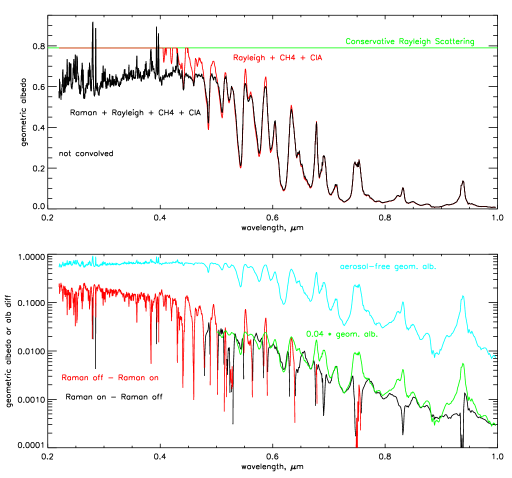
The effect of Raman scattering on Neptune’s aerosol-free geometric albedo is illustrated in Fig. 10, where spectra including polarization are shown for three calculations of increasing complexity, first with only Rayleigh scattering, then including also molecular absorption, and finally including Raman scattering. The calculations were started at 0.2 m, and are accurate to better than 1% at wavelengths beyond 0.22 m. Experiments with different starting wavelengths show that an accuracy of 1% or better can be achieved at a given short wavelength by starting the calculation at a corresponding wavenumber that is higher by twice the wavenumber shift of the -branch transition. This relatively small starting offset is effective because of the steep gradient in the solar spectrum at short wavelengths (see Fig. 6). The calculation was carried out with a step size of 17.78 cm-1, using a solar spectrum with a nominal resolution of 35 cm-1. With only conservative Rayleigh scattering, Neptune’s geometric albedo would be a wavelength-independent 0.791 (Sromovsky 2004). Adding methane absorption and collision-induced hydrogen absorption (CIA) only reduces the albedo at wavelengths beyond 0.4 m. Raman scattering produces profound effects throughout the UV and most of the visible spectrum.
Besides the introduction of sharp spectral features, Raman scattering also reduce Neptune’s baseline geometric albedo by nearly 25% in a clear atmosphere. In Fig. 10 the albedo decreases (shown as red) appear mostly at shorter wavelengths, but also appear in the vicinity of most of the local peaks in the near-IR reflectivity. The albedo gains (shown as black) occur not just at the deep minima in the solar spectrum, but also at the absorption maxima in the CH4 spectrum, which correspond to minima in the reflectivity spectrum.
We find that the fill-in of the reflectivity minima in the near IR is only about 4% of the geometric albedo. This is in sharp contrast to the Cochran and Trafton (1978) conclusion that in the cores of the strong CH4 bands at 0.86 m, 0.89 m and 1.0 m, nearly all of the photons that leave the atmosphere have been Raman scattered. However, their conclusion is a result of what we now know to be inappropriate assumptions concerning the amount and vertical distribution of methane. Their standard model had a constant mixing ratio of 0.005 relative to H2 throughout the atmosphere. This resulted in CH4 supersaturation for bar, by factors of 100 at the tropopause and more than 10 in the stratosphere. This resulted in a very low single scattering albedo of at 0.89 m, which even for a semi-infinite atmosphere would yield a very low geometric albedo of only 0.00036, using the single-scattering approximation for (Sromovsky 2004). That is about 20 times smaller than the geometric albedo we computed for our assumed CH4 profile, which never exceeds saturation levels and is limited to 3.510-4 in the stratosphere. Our distribution leads to much more scattering at the center of the disk and significant limb brightening (Sromovsky 2004), while the uniform mixing ratio of Cochran and Trafton makes the atmosphere dark at all view angles.
5.4. Comparison with other Raman Calculations
The earliest accurate calculation of a Raman spectrum relevant to Neptune was by Cochran and Trafton (1978) for a pure H2 atmosphere assuming an equilibrium population of ortho and para states. Their most relevant case is for 500 km-amagats of H2 over an opaque cloud layer (of unspecified but apparently high albedo). That amount of H2 corresponds to an atmospheric depth of approximately 6 bars, which is deep enough to approach semi-infinite behavior only for 0.34 m. At 0.5 m the surface albedo can make a difference of 0.25 in geometric albedo. Using 2/3 of the Ford and Browne (1973) Raman cross sections to approximate the values used by Cochran and Trafton, we computed geometric albedo values for a He-free atmosphere with a unit-albedo Lambertian surface placed at the 6-bar level, and ignored polarization. This spectrum, smoothed to a resolution of 5-nm, is displayed in Fig. 11 where it compares well with the even lower resolution spectrum of Cochran and Trafton.
The other prior calculation displayed in Fig. 11 is due to Savage et al. (1980), who used the same iterative computational scheme first presented by Cochran and Trafton (1978). According to Savage et al. , they used the Ford and Browne (1973) Raman cross sections that we used, but ignored polarization and assumed a pure H2 atmosphere, which was deep but of unspecified depth. In spite of their use of different Raman cross sections, the Savage et al. and Cochran and Trafton results agree with each other and with our calculations using 2/3 of of the Ford and Browne cross sections, raising questions about what cross sections were actually used by Savage et al. (1980). Our calculation with the Ford and Browne cross sections, and other conditions being the same, are shown as the thinner dot-dash curve in Fig. 11. Clearly, this spectrum is not compatible with the Savage et al. results. All these calculations have a stronger upward slope than we obtained for a truly deep atmosphere (Fig. 10) because the surface reflection becomes more visible at longer wavelengths. This can be seen from the difference between calculations for zero and unit surface albedos, which are shown in the figure. Other effects occur when we carry out more realistic calculations. The presence of helium dilutes the Raman absorption somewhat, producing about a 2% increase in the baseline value; using the correct Raman cross sections causes an albedo decrease of about 0.02-0.03 (a 3-5% decrease); and polarization increases the geometric albedo by about 0.04 (Sromovsky 2004) (a 6.7% increase). The approximate net result is a very small difference between the accurate calculation with polarization and the earlier H2-only calculations without polarization.

5.5. Comparison with Observed Spectra
The International Ultraviolet Explorer (IUE) made full-disk observations of Neptune during 2-5 October 1985 (days 275-277) at a phase angle of 1.87∘and a sub-earth latitude of -19.95∘planetographic (-19.325∘centric). Wagener et al. (1986) converted these observations to geometric albedo assuming an equatorial radius of 25240 km and an oblateness of 0.021, which are average stellar occultation results referring to a pressure of 1 microbar (French 1984). Using measurements of 24764 km and 0.01708 (Davies et al. 1992), which refer to the 1-bar level, we obtain a conversion factor of 1.035 for adjusting the Wagener et al. albedo values (this disagrees with the factor of 1.047 used by Courtin (1999)). We did not make a correction for phase angle, though that might increase their values by as much as 1% if the phase curve at UV wavelengths is similar to that observed at longer wavelengths (Sromovsky et al. 2003). The adjusted IUE results are compared with our clear-sky and Haze I Neptune spectra in Fig. 12, where error bars indicate the absolute uncertainty estimates due to Wagener et al. (1986). The IUE results are 5% to 10% below the theoretical clear-sky calculated spectrum, generally showing the smaller difference at shorter wavelengths (0.21-0.23 m) and the best defined and larger differences at longer wavelengths (0.29-0.33 m), which is likely due to an absorbing high altitude haze. Our Haze I model calculations match the IUE observations generally well within the IUE error bars. If we had neglected polarization, the model calculations would drop about 5%, making the clear-atmosphere model the best fit near 0.25 m. In this spectral range, polarization makes the difference between needing haze absorption and not needing it.
The Faint Object Spectrograph (FOS) observed Neptune at a phase angle of 1.22∘ and a sub-earth latitude of -24.78∘ planetographic on 19 August 1992 using apertures of 0.3′′, covering 21-36∘S, and 1.0′′, covering 3-35∘S. Because these apertures are smaller than Neptune’s 2.4′′ disk and placed near the middle of Neptune’s disk, the observed I/F and the relative amplitudes of Raman spectral features are increased relative to what would be observed for a full-disk average (shown in Sec. 7). Courtin (1999) obtained uncalibrated geometric albedo spectra by dividing FOS flux spectra by a solar flux spectrum measured by the UARS SOLSTICE instrument (Rottman et al. 1993; Woods et al. 1993). The FOS results we use are the 1-arcsec spectra degraded to a resolution of 1 nm to improve the signal/noise ratio (shown in Courtin’s Fig. 2). Courtin performed a radiometric calibration by matching his 0.22-0.33 m FOS spectra to full-disk 0.3 - 1.0 m groundbased spectrum of Karkoschka (1994), obtained during 23-26 July 1993 at a phase angle of 0.4∘. The FOS observations thus have the same 4% absolute uncertainty as the Karkoschka (1994) reference spectrum. The FOS noise level varies from 0.4% at 0.33 m to 1% at 0.26 m. Courtin’s Neptune spectrum is compared to our clear-sky and Haze I calculations in Fig. 13. Our calculations as a function of view angle were integrated over approximately the same field of view as the FOS observations to account for the increased Raman effect near normal view angles. We then convolved them to a final resolution of 1 nm and scaled this average spectrum to match our calculated geometric albedo spectrum in the wavelength range from 0.31 m to 0.33 m, to simulate the calibration procedure used by Courtin. Note the excellent agreement between the shapes and amplitudes of the calculated spectral features for the Haze I model and those measured by the FOS. The most glaring exceptions (a and b in the figure) appear to be artifacts in the FOS spectrum. These anomalies are not present in the overlapping portion of the Karkoschka spectrum, which is in good agreement with the calculated spectrum. The spikes c and d in the ratio spectrum are at points where the I/F spectrum has very sharp gradients, and could be removed by a slight wavelength shift. The FOS/Haze I ratio spectrum generally agrees with the IUE/Haze I ratio shown in Fig. 12, indicating that haze absorption may be depressing the reflectivity by about 6%-10% below the theoretical value for a clear Neptune atmosphere in the 0.23-0.27 m range, with increasing absorption indicated at longer wavelengths.


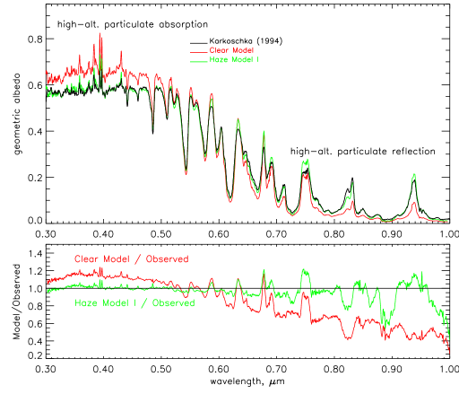
Figure 14 compares clear-atmosphere and Haze I model calculations with the disk-integrated groundbased spectra of Karkoschka (1994). Between 0.35 m and 0.45 m the observations are about 13% below the clear-atmosphere calculations, indicating a presence of an absorbing haze that is even more influential than at shorter wavelengths. This behavior suggests that the haze extends deep enough into the atmosphere that it becomes more influential as the molecular scattering optical depth above it decreases with increasing wavelength. This is qualitatively consistent with microphysical models of Moses et al. (1995), which suggest that haze opacity increases down to the 870 mb level. It is also roughly the character of our Haze I model, which is shown to provide good agreement with Karkoschka’s observations, although the computed amplitudes of the Raman spectral features are somewhat larger than the observations in several cases. This discrepancy might mean that more aerosol opacity is needed in the 1-3 bar level, or that there is a slight difference in the effective spectral resolution of the observations and the calculations. At longer wavelengths, the high observed albedo values in the deep CH4 bands at 0.8 m and 0.9 m, indicate that there is also particulate scattering at high altitudes, which is not included in either of the haze models. Much of that contribution probably comes from discrete bright features seen in Voyager, HST, and groundbased images. Effective pressure estimates for such features range from 23 mb to 60 mb at 30-40∘ N, 100-230 mb at 30-50∘ S, and 170 mb to 270 mb near 70∘ S (Sromovsky et al. 2001b; Gibbard et al. 2003). The effective fractional coverage of bright high altitude clouds required to explain the albedo in deep CH4 bands appears to be about 0.5% to 1% for an upper cloud at 150 mb (Sromovsky et al. 2001a). The effective fractional coverage of a coexisting 1.3-bar cloud is 1% assuming a unit-albedo Lambertian reflector.
The observed albedo in the window regions at 0.825 m and 0.935 m is also significantly above the clear-sky calculation, suggesting a significant aerosol contribution that could be at mid to deep levels, which is largely satisfied by the 1.3-bar and 3.8-bar clouds in the Haze I model. The excess I/F calculated in the window regions at 0.59 m, 0.63 m, 0.68 m, and 0.75 m, can be substantially reduced by increasing the CH4 continuum absorption by amounts comparable to Karkoschka’s stated continuum uncertainty. It could also be reduced by decreasing the single-scattering albedo of the cloud aerosols. The observations seem to show much less of the collision-induced absorption in the 0.8-0.83 m region than is evident in the calculations. Another way to describe this difference is to say that there is an imbalance in the 0.83 and 0.94 m window regions that is evident in the calculation, but not in the observations. That imbalance may be due to an error in the CH4 absorption coefficients. If we add to Karkoschka’s standard coefficients the continuum absorption uncertainty, we actually obtain very similar albedo values in these two windows.
5.6. Spectral Evidence of the Ortho/Para Ratio
Because the Raman cross sections are larger than the cross sections (Fig. 2), the ortho/para ratio will have an effect on the Raman features observed in Neptune’s reflection spectrum. The largest difference in ortho/para ratios for equilibrium and normal H2 occur near 100 mb (Fig. 1), and thus associated spectral variations are more likely at short wavelengths where this region is near the level (Fig. 4). Calculations (Fig. 15) show that the largest difference is for the peaks at 0.280 m and 0.2852 m, which are about 5% larger for equilibrium H2. The overlay of FOS observations suggests better agreement with equilibrium H2, as concluded by Courtin (1999), although the relative size of the smaller peak is very dependent on the effective resolution of the observations and both peaks have amplitudes that depend on view angle. And since the FOS observations cover only the central disk, it is not strictly valid to compare them to geometric albedo observations. Uncertainties in the wavelength scale and effective resolution of the FOS observations arise from comparisons with overlapping groundbased observations of Karkoschka (1994), which show significantly less spectral modulation in the 0.3-0.33 m overlap region, as noted earlier. The presence of an absorbing haze and high-altitude discrete clouds also affects these peaks. Thus it seems premature to make a strong conclusion based on these observations. However, Courtin’s (1999) result that =0.880.23 is based on higher resolution observations than those shown in Fig. 15, and was derived after special processing to minimize wavelength errors. Courtin’s results are also compatible with independent conclusions by Baines and Smith (1990) and Conrath et al. (1991) that the ortho/para ratio for Neptune is near thermal equilibrium.

6. Approximations of Raman Scattering
6.1. The Karkoschka Correction
Karkoschka (1994) presented a method for transforming spectra between Raman and non-Raman forms based on the assumption that the measured geometric albedo spectrum can be well approximated by a linear combination of terms involving offset versions of the “physical” spectrum , which is the reflectivity spectrum without Raman scattering. The mathematical expression of this method is
| (39) |
where is here the solar photon spectrum, is the fraction of photons not Raman scattered, is the fraction undergoing transition , and where Equation 39 can be inverted to obtain the Raman-free “physical” spectrum from the observed spectrum using as a first guess, and then improving the guess using the iterative equation
| (40) |
for which four iterations are usually sufficient to converge on for a given set of fractions. Karkoschka assumed a power law -dependence for , then used minimum roughness of the fitted spectrum for 0.31 m 0.405 m as the criterion for picking the optimum fractions and exponent.

| -range | RMS | ||||||
|---|---|---|---|---|---|---|---|
| Spectrum | (m) | DEV | |||||
| Clear Sky | 0.31-.405 | 0.1000.005 | 0.0650.007 | 0.0500.005 | 0.0850.005 | -0.800.05 | 0.93% |
| Clear Sky | 0.23-.405 | 0.1000.005 | 0.0700.005 | 0.0300.005 | 0.0910.005 | -0.500.07 | 1.47% |
| Haze II | 0.31-.405 | 0.0500.005 | 0.0650.005 | 0.0300.005 | 0.0570.005 | -0.550.05 | 0.44% |
| Haze II | 0.23-.405 | 0.0350.003 | 0.0600.004 | 0.0300.005 | 0.0850.005 | -0.350.06 | 0.90% |
| Haze II (inv) | 0.23-.405 | 0.0600.020 | 0.0600.004 | 0.0300.003 | 0.0650.005 | -0.350.05 | 0.58% |
| K94 Coeff. | 0.31-.405 | 0.0350.015 | 0.0600.01 | 0.0250.015 | 0.050 | -11 |
NOTE: Fractional values are given at 400 nm. Values at other wavelengths are proportional to . Haze II (inv) refers to the inversion of fit parameters from the Raman spectrum only, rather than starting with the Raman-free spectrum. In this case RMS DEV is relative to the smoothed spectrum, which was smoothed with a boxcar of 0.71 nm. The last row is from Karkoschka (1994).
We first investigated how well the proposed model could fit Raman spectral calculations and how the fitted constants related to Raman scattering cross sections. We considered both a clear-atmosphere model and a model with haze and cloud contributions. We first fit the fractional parameters and wavelength dependence exponent by minimizing the RMS deviation between the Karkoschka model and the calculated spectrum, first over the 0.31-0.405 m range used by Karkoschka and also over the wider 0.23-0.405 m range. The results are summarized in Table 5. Note that our fit results are comparable to those of Karkoschka, especially when applied to a hazy atmosphere. Although we were able to obtain good fits over the limited spectral ranges (RMS deviations of 0.44% and 0.9% for the haze/cloud model, and 0.93% and 1.47% for clear sky model), the fits did not accurately match the observed spectrum at slightly longer wavelengths, especially where CH4 absorption was present. The weak CH4 bands in the Karkoschka conversion of the physical spectrum were much stronger than the corresponding bands in the correct Raman calculation. This is understandable as a consequence of the nonlinear relationship between I/F and single-scattering albedo. A small absorption added to a conservative atmosphere can have a much larger fractional effect than it does when added to an absorbing atmosphere. For example, adding to a Rayleigh atmosphere with changes from 1.0 to 0.997, which decreases the I/F from 0.791 to 0.699, a 9% drop. But if the I/F is already at 0.559 due to Raman absorption, adding the same CH4 absorption as before would change from 0.975 to 0.972, producing only a 2% drop in I/F. Confirming Karkoschka’s fit results, we find that the vibrational coefficient () is about twice the size of the coefficient for the rotational contribution (), even though its Raman cross section is somewhat smaller (Table 3). Since we use these cross sections to compute the spectra, the fit results do not suggest that there is something wrong with the cross sections. A large part of this result comes from the fact that the vibrational coefficient represents the average of ortho and para contributions, while the individual and contributions are each multiplied by fractions that decrease their relative contributions by roughly a factor of two (for , see Eq. 3 and Fig. 1). Additional factors are discussed in Sec. 5.1.
We next consider how well Karkoschka’s method is able to remove Raman scattering effects from a spectrum that includes Raman scattering. We inverted our model Raman calculations using the inversion method based on Eq. 40. The retrieved parameter values for the Haze II test case are given in Table 5. As illustrated in Fig. 16, we found pretty fair agreement between the true Raman-free spectrum and inverted spectrum for the haze/cloud case when we used the 0.23-0.405 m range for the fitting, although our inverted spectrum is offset about 0.01 albedo units above the true spectrum, and the inverted parameters differ somewhat from the best-fit parameters. Using the 0.23-0.405 m spectral range yielded a smoother inverted spectrum but a larger offset albedo of 0.03. Much worse results were obtained with the clear sky model, which has larger Raman features that are not as well fit by Karkoschka’s empirical model. As expected, we found that the features due to weak CH4 bands were much smaller in the transformed spectra than in the true physical spectra. Thus, estimates of CH4 absorption coefficients using spectra corrected in this way will be significantly below the true absorption level.
Karkoschka’s method has several physical flaws that limit its applicability. Multiple scattering is one effect that is not accounted for but can be significant (see Sec. 5.1). Another problem with the physics assumed in Eq. 39 is that the contribution at the present wavenumber is not necessarily proportional to the geometric albedo at the upward shifted wavenumber. In fact, the proportionality constant also depends on the vertical distribution of the scattered photons in relation to the vertical distribution of opacity at the scattered wavelength. The Karkoschka forward method also is not generally applicable to spatially resolved observations because the amplitude of Raman effects depends on view angle as well as local aerosol structure. The useful spectral range for the Karkoschka correction is also rather limited, probably to wavelengths less than about 0.405 m, partly because it does not properly modify weak CH4 absorption bands.
6.2. The Wallace Approximation
The approximation suggested by Wallace (1972) is a modification of the molecular single scattering albedo of the atmosphere by treating rotational transitions as extra sources of scattering and the vibrational transition as a pure absorption. This can be expressed in terms of cross sections as follows:
| (41) |
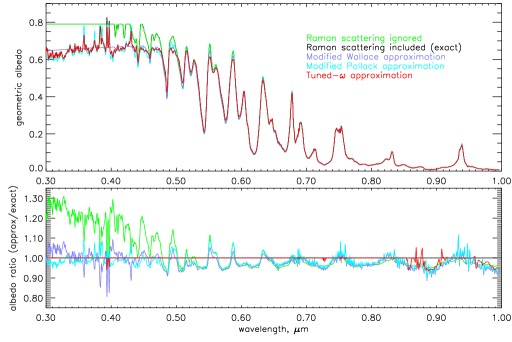
where is the Rayleigh scattering cross section, is the total cross section for absorption by CH4 and CIA by H2, is the combined cross section for rotational Raman transitions, is the cross section for vibrational Raman transitions, and where for the original Wallace approximation. For a clear Neptune atmosphere, we find that the original Wallace approximation provides a crude match to the low resolution baseline of the spectrum, but is generally 5% to 10% low and of course does not produce characteristic Raman spectral features. A few detailed calculations by Wallace (1972) at 0.2 m and 0.4 m also indicated that his approximation was about 5% low. The Wallace approximation error is nearly zero in the near-IR CH4 windows, but is about 4% low in the CH4 absorption bands, which is about what would be expected if Raman scattering were ignored (see lower part of Fig. 17). Figure 17 displays a modified form of the Wallace approximation that boosts the I/F value by setting , which treats the vibrational cross section as 56.7% absorption and 43.3% scattering. This improves the overall agreement in the blue to orange part of the spectrum, but has little effect elsewhere. The Wallace approximation approaches the exact result when high clouds obscure most of the molecular scattering.
6.3. The Pollack Approximation
Pollack et al. (1986) approximated Raman scattering contributions from shorter wavelengths by scaling the Raman scattering cross section at the reflected wavelength by the ratio of solar irradiance at the source wavelength to that at the reflected wavelength. Generalizing this approach to include more than one transition, the molecular single-scattering albedo in this approximation can be written as:
| (42) |
where , is a function of that can be empirically adjusted to compensate for some of the complexities that are glossed over by this concept, and the upper bound of 1 is used to avoid energy conservation problems. Setting , and omitting the rotational transitions completely, would reduce this to Pollack’s original suggestion, while setting and would reduce this to the Wallace approximation. A problem with Pollack’s original formulation was that it resulted in at some wavelengths, as noted by Courtin (1999), which leads to instability in the solution of the radiation transfer equation. Another problem is that it considered only the vibrational transition, which alone would be unable to generate the ghost features arising from the rotational transitions. The form given in Eq. 42 has the capability to fit all the main ghost features and has the potential, with tuning of the form of , to yield the correct baseline value as well. It also has an advantage over Karkoschka’s correction, in that it is introduced at a more fundamental physical level that is naturally modified by the presence of aerosols. However, wherever the geometric albedo exceeds the value for a conservative Rayleigh atmosphere of 0.7908 (Sromovsky 2004), even will not be able to reproduce the albedo value. This problem can be reduced by working at lower spectral resolutions for which these extreme peak amplitudes become reduced below 0.7908.
Preliminary calculations with this approximation used the three transitions given in Table 4, with and the same for all transitions. We found that making the constant = 0.875 for all produced a reasonably good match to the baseline level of geometric albedo, but generated spectral modulations that were too large. To limit these modulations, we used an exponential function to limit the effect of the spectral irradiance ratio, i.e. we used , which is for small and approaches for large values of . We found that provided a reasonable fit to the Raman spectral features and to the baseline level, as shown in Fig. 17. While this is certainly an improvement over the Wallace approximation, and does reproduce many of the spectral features associated with Raman scattering, it does not do so consistently and accurately enough to use for interpreting those features. Like the Wallace approximation, it also fails to improve geometric albedo accuracy for 0.47 m. Both Wallace and Pollack modifications to the single-scattering albedo seem to be far less effective in regions where CH4 absorption is important. Since the actual source function depends on the light level in the atmosphere, which may have a spectral shape that is very different from the incident solar spectrum, it is not appropriate to use the solar spectral ratio as a scale factor in spectral regions with strong CH4 absorption. The following method goes part of the way in solving this problem.
6.4. Approximation of Raman Scattering by Spectral Tuning of
The following describes a new approximation of Raman scattering that uses a different kind of modification of the molecular single scattering albedo. Instead of using a constant factor or the solar spectral ratio to modify the molecular single-scattering albedo, this approximation uses a -dependent multiplier that is tuned to minimize the difference between simulated and exact Raman calculations of geometric albedo for an appropriate model atmosphere. The fundamental relation used is from Sromovsky (2004):
| (43) |
where is the geometric albedo including polarization contributions and is the single scattering albedo of a semi-infinite Rayleigh atmosphere. This equation is inverted numerically to provide a function so that a given geometric albedo can be related to an equivalent single-scattering albedo of a semi-infinite Rayleigh atmosphere. Starting with a Raman-free calculation producing a spectrum , and a true Raman calculation producing a spectrum , we use the inverse transform to compute equivalent single-scattering albedos and . Noting that , we then attribute the difference between the equivalent inverse single scattering albedos as due to a difference in the effective absorption due to Raman scattering. Thus we are led to the approximation for modifying the single scattering albedo of the molecular scatterings that simulate true Raman scattering, namely,
| (44) |
where is the single-scattering albedo simulation of Raman scattering on the prior iteration, is the effective semi-infinite single scattering albedo obtained from the spectrum generated using for the molecular scattering. Because Neptune’s atmosphere has a vertically inhomogeneous CH4 distribution, and thus will not satisfy Eq. 43, it is necessary to iterate a few times to achieve convergence. On the first iteration, we have and . The molecular single-scattering albedo spectrum that results is , which reduces to when .
The nearly perfect agreement between the geometric albedo computed with Raman scattering and the approximation using a tuned single-scattering albedo is shown in Fig. 17. Unlike the previously discussed approximations, it does provide useful accuracy for 0.45 m. Like the other approximations, it cannot reproduce the peaks that exceed the I/F for a unit geometric albedo. While the modified single-scattering albedo can exceed unity, or even go negative, that does not lead to problems as long as the other contributors to the scattering process lead to a combined single-scattering albedo .
The important question is whether this approximation or any of the others that are similarly constructed, are useful with clouds present, and for center-to-limb scans. Because all of these approximations that modify single-scattering albedos really lack the essential physics of the Raman scattering process, it is doubtful whether they can have much utility in situations for which they have not been tuned. A partial test of this utility is the degree to which they can simulate the angular variation of Raman scattering, which is described in the next section. Section 8 compares their performances when haze and cloud aerosols are present.
7. Angular Dependence of Raman Scattering Effects
Raman scattering effects on Neptune’s I/F spectrum at zero phase angle are strongest near the center of the disk (zero zenith angle) and weakest near the limb (Fig. 18). The errors obtained by ignoring Raman scattering (not shown) are quite substantial at moderate view angles, especially at short wavelengths and at high spectral resolution, ranging from about 20 to 60% in the 0.25-0.3 m range at a zenith angle of 8.1∘. At view angles of 60∘, the fractional errors are comparable to those seen for the geometric albedo. As noted for the geometric albedo, errors 4% are seen in the deep CH4 bands, with very little error seen in the near-IR window regions. In the longer wavelength bands, the fractional error does not improve much near the limb, unlike the error at shorter wavelengths, which decreases substantially.
The modified Pollack approximation helps considerably in reducing errors at short wavelengths (Fig. 18). The extreme error near the central disk drops from 62% to 14% and the RMS error from 19% to 4%. At 63∘ the RMS error drops from 8.8% to 2.2%. But at long wavelengths, the Pollack approximation actually makes things slightly worse in the middle of strong absorption bands, probably because the vertical location of Raman photons becomes more critical to the resulting I/F level. Overall, the modified Pollack approximation has value in modeling a variety of observations. It is far better than ignoring Raman scattering and is roughly twice as accurate as the modified Wallace approximation. However, using the modified Pollack approximation can lead to substantial errors in limb-darkening profiles, depending on the wavelength that is considered. Sample profiles are shown in Fig. 19.
Under most conditions, the tuned- approximation is even more accurate than the modified Pollack approximation, as evident from comparison of spectra at the three sample angles (Fig. 18) and from a comparison of center-to-limb scans at sample wavelengths (Fig. 19) . The extreme error near the central disk drops to 10.3% and the mean and RMS deviations to only -1.1% and 1.2%, with comparable results at 63∘ view angles. The worst errors are seen at large view angles. At 85.7∘ , the extreme error increases to 24% and the mean and RMS errors increase to 2.6% and 3.3%. But most of these errors occur in the CH4 bands beyond about 0.53 m. If restricted to 70∘ view angles and 0.85 m, this approximation is remarkably effective, with errors rarely exceeding a few percent.
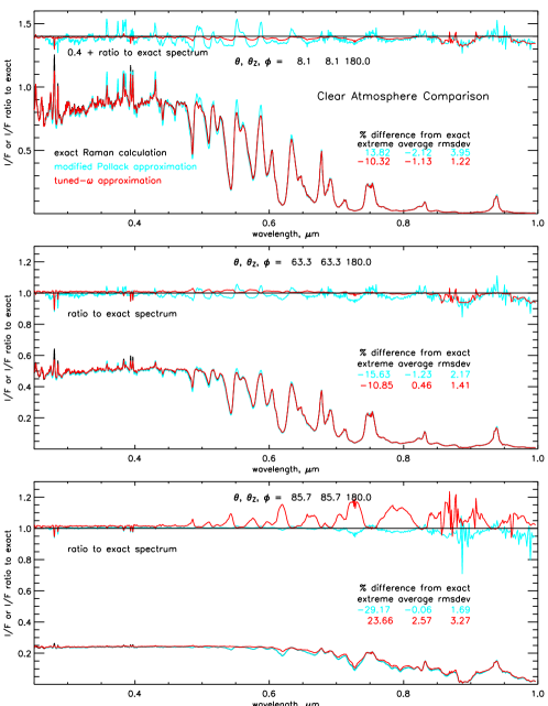
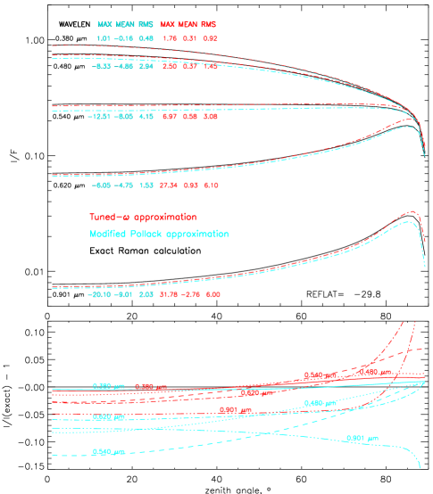
8. Effects of Aerosols on Approximation Performance
Calculations for the Haze II atmospheric model containing the cloud and haze aerosols described in Sec. 4.2 are presented in Fig. 20, where the calculation that ignores Raman scattering is compared to the Raman calculation and to the modified Pollack and tuned- approximations. At UV-visible wavelengths we see that the size of the Raman features is substantially reduced by the addition of a high altitude absorbing haze, which also depresses the baseline reflectivity as needed to approximately match observations. The net effect of Raman scattering on the baseline reflectivity is also reduced substantially compared to its effect in a clear atmosphere. This is another example of the nonlinear effects of adding absorption (see discussion in Sec. 6.1). The effects of the cloud layers are most easily seen at longer wavelengths where the I/F in window regions and regions of intermediate methane absorption are increased substantially compared to that computed for a clear atmosphere.
The tuned- approximation is seen to perform well for 0.6 m, where haze effects dominate, but is biased about 5% too high in the strongly absorbing regions at longer wavelengths, although remaining quite accurate in window regions. This is not too surprising, because the tuning in these regions is involves a delicate balance between large molecular absorption and large corrections of that absorption to simulate the Raman-scattered contributions. As vertical structure is changed from that used for tuning, the tuning can be easily upset.
The modified Pollack approximation performs somewhat worse at UV-visible wavelengths than it did for the clear atmosphere case (Fig. 17). The overall negative bias seen here could probably be largely eliminated by adjusting the parameters of the factors in Eq. 42. That would do much to reduce the positive errors in the window regions beyond 0.45 m or the negative errors in the absorbing regions. These are inherent in the physical model on which the Pollack approximation is based. Overall, this approximation is less upset by the presence of the cloud layers than is the tuned- approximation.
A comparison of these two approximations at three different view angles is presented in Fig. 21. We see that the tuned- approximation is much better near the central disk, and effective at all wavelengths. It is also effective at all angles for wavelengths less than 0.47 m. But at longer wavelengths, errors in the regions of strong methane absorption grow with increasing view angle, making the modified Pollack approximation better for view angles beyond about 50∘ .
The Karkoschka approximation was not included in this particular comparison because is not useful for spatially resolved observations, especially those with variable cloud structure, unless the model coefficients are changed for each view angle and structure. Even then, the serious problems at 0.4 m (see Fig. 16) also reduce its utility, even for disk-average analyses.
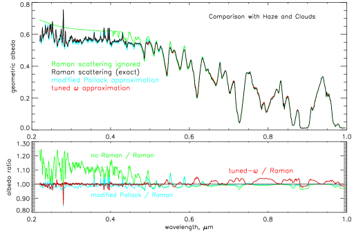
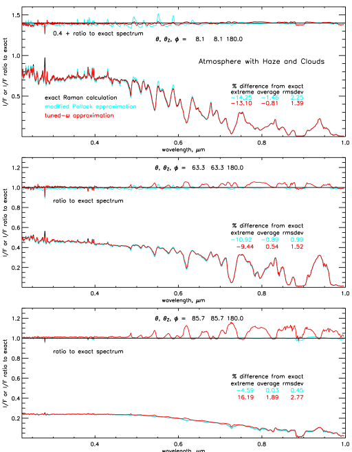
9. Summary and Conclusions
Major results of this investigation can be summarized as follows:
- (1) Radiation Transfer.
-
Procedures for modifying the Evans and Stevens (1991) vector radiation transfer code to handle Raman scattering are described and justified. Equations are provided for the Raman differential generators. The use of a Raman source matrix facilitates the computation of the first spatially resolved Raman scattering spectra for Neptune. Validation of the code is obtained by demonstration of photon conservation, comparison with prior low-resolution calculations, and comparison with HST and groundbased observations.
- (2) Basic Effects on Geometric Albedo.
-
Raman scattering reduces the baseline geometric albedo of a semi-infinite conservative Rayleigh scattering atmosphere by about 25% from the value of 0.791 it would otherwise have. In the presence of a high-altitude absorbing haze, the effect of Raman scattering is reduced by about a factor of two. The well known sharp positive spectral peaks from fill-in of absorption lines in the solar spectrum can greatly exceed the Rayleigh conservative limit. For photons introduced at 228 nm, the transition source function for the first scattering has a broad peak near 300 mb; after further scattering photons move deeper into the atmosphere and leak out the top, moving the peak of the source function further downward after each scattering.
- (3) Near-IR Effects.
-
For a clear atmosphere about 4% of the light in the deep methane bands in the near-IR is due to Raman scattering, while the near IR window regions are almost unaffected by Raman scattering. The conclusion of Cochran and Trafton (1978) that the light in the deep methane bands is almost entirely Raman scattered is a result of their assumption of what are now known to be excessively high methane mixing ratios in the stratosphere.
- (4) Multiple Scattering.
-
The calculated history of monochromatic incident photons shows that multiple Raman scattering is quite significant in a conservative Rayleigh scattering atmosphere, where the Raman absorption process can compete with the loss to space. In one example calculation, only 40% of the Raman scattered photons exiting the atmosphere experienced only one Raman scattering.
- (5) Angular Variation.
-
At low phase angles spatially resolved Raman spectra show that Raman spectral features are enhanced at near the center of the planetary disk and suppressed at the limb. We also found that approximations that work reasonably well in matching accurate disk-integrated calculations do not do as well in matching observations in specific directions, especially at large view angles.
- (6) Comparison with Observations.
-
Aerosol-free models of Neptune’s spectrum correlate well with observed spectral features, but confirm a need for haze absorption to reduce the baseline geometric albedo and to reduce the amplitude of spectral modulations induced by Raman scattering. IUE full-disk observations, adjusted to account for current knowledge of of Neptune’s size, have a baseline offset of 6% in the 0.24-0.26 m range, increasing to about 10% in the 0.30-0.32 m range, both of which are fit well by our Haze I model, containing 0.2 optical depths (at 0.5 m) of a UV absorbing haze of 0.2-m radius particles uniformly mixed between 0.1 and 0.8 bars. FOS observations between 0.22 and 0.29 m, have a similar offset and high-resolution spectral structure that is also well fit by our Haze I model. Groundbased disk-integrated observations between 0.35 and 0.45 m have a baseline offset that is 13% below the clear-atmosphere calculation which is well matched by our Haze I calculation, although several of the spectral features are seen to have greater amplitude in the calculations than in the observations. We consider the Haze I model to be a sample calculation, not a tightly constrained fit.
- (7) Karkoschka correction.
-
The Karkoschka (1994) method of applying Raman corrections to calculated spectra and removing Raman effects from observed spectra is shown to be relatively accurate under restricted conditions, but has practical limitations for problems involving spatially resolved observations or for m. His Raman removal algorithm undercorrects the depths of weak CH4 absorption bands, and thus corresponding absorption coefficients derived from such spectra (Karkoschka 1994; 1998) will need some revision. The relatively large amplitude of the Q-branch contributions found by Karkoschka is shown to be consistent with current estimates of Raman cross sections, not an indication that they are in error.
- (8) Wallace Approximation.
-
We agree with Wallace (1972) that his suggested approximation yields geometric albedos that are typically 5% lower than an accurate calculation. A generalization of this approximation that counts part of the vibrational cross section as contributing to scattering can remove this bias. This approximation does not help reduce errors in the strong CH4 bands and is mainly useful at low resolution and for 0.45 m.
- (9) Pollack Approximation.
-
The initial form of the approximation suggested by Pollack et al. (1986) generates serious errors. But generalizing it to include rotational and vibrational transitions, enforcing energy conservation, and limiting the solar spectral ratio enhancement, can produce a relatively good approximation, except for 0.45 m, where ignoring Raman scattering is just as accurate.
- (10) Tuned- Approximation.
-
By tuning the absorption attributed to Raman scattering it is possible to make a non-Raman calculation match a true Raman calculation with virtually no error. If that matching is done with respect to geometric albedo, it will not match nearly as well for spatially resolved calculations. It is nevertheless the best approximation to use under cloud-free conditions for zenith angles less than 70∘ and wavelengths less than 0.85 m. It is the only one that provides improvements for 0.45 m, although is not very effective for 0.47 m when cloud layers of intermediate opacity are present.
Most of these conclusions apply with equal force to Raman scattering in the atmosphere of Uranus because of its similarity to Neptune in vertical temperature structure, gas composition, and relatively low aerosol loading. Conclusion (6) would need the most revision to accommodate differences in detailed observational results.
Acknowledgments
This research was supported by a grant from NASA’s Planetary Atmospheres program and in part by an Archive Research Grant from the Space Telescope Science Institute. I thank Pat Fry who helped with the installation of the original Evans and Stevens code and advised on FORTRAN debugging of modifications to it. I also thank Evans and Stevens for making their well written code available to the community, R. Courtin for providing tabular data files of his processed FOS observations, and two anonymous reviewers.
References
-
Allen, C. W. 1964. Astrophysical Quantities, 2nd Edition. 291 pages. Athlone Press, London.
-
Baines, K. H., and W. H. Smith 1990. The Atmospheric Structure and Dynamical Properties of Neptune Derived from Ground-Based and IUE Spectrophotometry. Icarus 85, 65-108.
-
Baines, K. H., H. B. Hammel, K. A. Rages, P. N. Romani, and R. E. Samuelson (1995) Clouds and hazes in the atmosphere of Neptune. In Neptune and Triton, D.P. Cruikshank, ed., Univ. of Arizona Press.
-
Baines, K. H., and H. B. Hammel 1994. Clouds, hazes, and the stratospheric methane abundance in Neptune. Icarus 109, 20-39.
-
Bétremieux, Y., and R. V. Yelle 1999. HST Detection of H2 Raman Scattering in the Jovian Atmosphere. Icarus 142, 324-341.
-
Bhagavantam, S., 1931. Raman effect in gases I. Some experimental results Ind. J. Phys. 6, 319-330.
-
Bhagavantam, S., 1942. Scattering of Light and the Raman Effect., 333 pages, Chemical Publishing Company Inc., Brooklyn NY.
-
Cabbanes, J. and A. Rousset 1936. Diffusion moléculaire: Mesure du facteur de dépolarization des raies Raman dans les gaz: Azote, oxygène, gaz carbonique. Comptes Rendus 202, 1825-1828.
-
Cochran, W. D., and L. M. Trafton 1978. Raman scattering in the atmospheres of the major planets. The Astrophys. J. 219, 756-762.
-
Conrath, B.J., T.C. Owen, and R.E. Samuelson 1993. Constraints on N2 in Neptune’s atmosphere from Voyager measurements. Icarus 101, 168-171.
-
Conrath, B. J., D. Gautier, G. F. Lindal, R. E. Samuelson, and W. A. Shaffer 1991. The helium abundance of Neptune from Voyager measurements. J. Geophys. Res. 96, 18907-18919.
-
Courtin, R. 1999. The Raman signature of H2 in the UV spectra of Uranus and Neptune: Constraints on the haze optical properties and on the para-H2 fraction. Planet. and Space Sci. 47, 1077-1100.
-
Davies, M., V. K. Abalakin, A. Brahic, M. Bursa, B. H. Chovitz, JK. H. Lieske, P. K. Seidelmann, A. T. Sinclair, and I. S. Tiuflin 1992. Report of the IAU/IAG/COSPAR Working Group on Cartographic Coordinates and Rotational Elements of the Planets and Satellites - 1991, Celestial Mechanics and Dynamical Astronomy (ISSN 0923-2958), 53, No. 4, p. 377-397.
-
Dlugach, E. G., and E. G. Yanovitskij 1974. The Optical Properites of Venus and the Jovian Planets. II. Methods and Results of Calculations of the Intensity of Radiation Diffusely Reflected from Semi-infinite Homogeneous Atmospheres. Icarus 22, 66-81.
-
Evans, K. F., and G. L. Stephens 1991. A New Polarized Atmospheric Radiative Transfer Model. J. Quant. Spectr. and Rad. Transfer 46, 413-423.
-
Farkas, A., 1935. Orthohydrogen, Parahydrogen and Heavy Hydrogen. Cambridge Univ. Press, London.
-
Ford, A. L., and J. C. Browne 1973. Rayleigh and Raman Cross Sections for the Hydrogen Molecule. Atomic Data 5, 305-313.
-
French, R. G. 1984. Oblatenesses of Uranus and Neptune. In Uranus and Neptune, NASA Conf. Pub. 2330, 349-355.
-
Gibbard, S. G., I. de Pater, H. G. Roe, S. Martin, B. A. Macintosh, and C. E. Max 2003. The altitude of Neptune cloud features from high-spatial-resolution near-infrared spectra. Icarus 2, 359-374.
-
Goody, R. M., Y. L. Yung 1989. Atmospheric Radiation, Oxford University Press, Oxford, New York.
-
Hansen, J. E. 1971. Multiple scattering of polarized light in planetary atmospheres. Part II. Sunlight reflected by terrestrial water clouds. J. Atmos. Sci. 28, 1400-1426.
-
Hansen, J. E., and L. D. Travis 1974. Light Scattering in Planetary Atmospheres. Space Science Reviews 16, 527-610.
-
Hinson, D. P., and J. A. Magalhães 1993. Inertio-gravity waves in the atmosphere of Neptune. Icarus 99, 142-161.
-
Hollas, M. 1992. Modern Spectroscopy, John Wiley & Sons, New York.
-
Hovenier, J. W. 1969. Symmetry relationships for scattering of polarized light in a slab of randomly oriented particles. J. Atmos. Sci. 26, 488-494.
-
Hu, Y.-X., B. Wielicki, B. Lin, G. Gibson, S.l-C. Tsay, K. Stamnes, and T. Wong 2000. -Fit: A fast and accurate treatment of particle scattering phase functions with weighted singular-value decomposition least-squares fitting. J. Quant. Spectr. and Rad. Transfer 65 681-690.
-
Karkoschka, E. 1994. Spectrophotometry of the jovian planets and Titan at 300- to 1000-nm wavelength: The methane spectrum. Icarus 111, 174-192.
-
Karksochka, E. 1998. Methane, ammonia, and temperature measurements of the Jovian planets and Titan from CCD-spectroscopy. Icarus 133, 134-146.
-
Karkoschka, E. and M. Tomasko 1992. Saturn’s Upper Troposphere 1986-1989. Icarus 97, 161-181.
-
Kattawar, G. W., and C. N. Adams 1971. Flux and Polarization Reflected from a Rayleigh-scattering Planetary Atmosphere. Astrophys. J. 167, 183-192.
-
Kurucz, R. L. 1993. Smithsonian Astrophysical Obsevatory CD ROM No. 13.
-
Lindal, G.F. 1992. The Atmosphere of Neptune: An analysis of radio occultation data acquired with Voyager 2. Astron. J. 103 , 967-982.
-
Massie, S. T., and D. M. Hunten 1982. Conversion of para and ortho Hydrogen in the Jovian Planets. Icarus 49, 213-226.
-
Mishchenko Th, M. I., A. A. Lacis, and L. D. Travis 1994. Errors induced by the neglect of polarization in radiance calculations for Rayleigh-scattering atmospheres. J. Quant. Spectr. and Rad. Transfer 51, 491-510.
-
Moses, J. I., K. Rages, and J. B. Pollack 1995. An Analysis of Neptune’s Stratospheric Haze Using High-Phase-Angle Voyager Images. Icarus 113, 232-266.
-
Neckel, H. and D. Labs 1984. The solar radiation between 3300 and 12500 Å. Solar Phys. 90, 205-258.
-
Parthasarathy, S. 1951. Light scattering in gases. Indian J. Phys. 25, 21-24.
-
Penndorf, R. 1957. Tables of the refractive index for standard air and the Rayleigh scattering coefficient for the spectral region between 0.2 and 20 m and their application to atmospheric optics. J. Opt. Soc. Am. 47, 176-182.
-
Placzek, G., 1959. Rayleigh and Raman scattering, pp. 206, University of California, Lawrence Radiation laboratory (Livermore, CA); [translated from Handbuch der Radiologie, Ed. E. Marx, Vol. 6, part II, end ed., (Akademische Verlagsgesellschaft, Leipzig, 1934), pp. 205-374]
-
Pollack, J. B., K. Rages, K. H. Baines, J. T. Bergstralh, D. Wenkert, and G. E. Danielson 1986. Estimates of the Bolometric Albedos and Radiation Balance of Uranus and Neptune. Icarus 65, 442-466.
-
Pryor, W.R., R.A. West, K.E. Simmons, and M. Delitsky 1992. High-phase angle observations of Neptune at 2650 Åand 7500Å: Haze structure and particle properties. Icarus 99, 302-316.
-
Rottman, G. J., T. N. Woods, T. P. Sparn 1993. SOLar-STellar Irradiance Comparison Experiment I: 1. Instrument design and operation. J. Geophys. Res. 98, 10667-10677.
-
Savage, B. D., W. D. Cochran, and P. R. Wesselius 1980. Ultraviolet Albedos of Uranus and Neptune The Astrophys. J. 237, 627-632.
-
Soris, C. E., and F. J. Evans 1999. Filling in of Fraunhofer and gas-absorption lines in sky spectra as caused by rotational Raman scattering. Applied Optics 38, 2706-2713.
-
Sromovsky, L. A., 2004. Effects of Rayleigh-scattering polarization on reflected intensity: A fast and accurate approximation for atmospheres with aerosols. Icarus in press.
-
Sromovsky, L. A., P. M. Fry, S. S. Limaye, and K. H. Baines 2003. The nature of Neptune’s increasing brightness: evidence for a seasonal response. Icarus 163, 256-261.
-
Sromovsky, L.A., P.M. Fry, K.H. Baines, and T. Dowling 2001a. Coordinated 1996 HST and IRTF Observations of Neptune and Triton II: Implications of Disk-Integrated Photometry, Icarus 149, 435-458.
-
Sromovsky, L.A., P.M. Fry, T. Dowling, K.H. Baines, and S.S. Limaye 2001b. Coordinated 1996 HST and IRTF Observations of Neptune and Triton III: Neptune’s Atmospheric Circulation and Cloud Structure, Icarus 149, 459-488.
-
Stamnes, K., S.-C. Tsay, W. Wiscombe, and K. Jayaweera 1988. Numerically stable algorithm for discrete-ordinate-method radiative transfer in multiple scattering and emitting layered media. App. Opt. 27, 2502-2509.
-
Sweigart, A. V. 1970. Radiative Transfer in Atmospheres scattering According to the Rayleigh Phase Function with Absorption. Astrophys. J. 182, 1-80.
-
Toon, O. B., C. P. McKay, T. P. Ackerman, K. Santhanam 1989. Rapid calculations of radiative transfer heating rates and photodissociation rates in inhomogeneous multiple scattering atmospheres. J. Geophys. Res 94, 16287-16301.
-
Wagener, R., J. Caldwell, and K-H. Fricke 1986. The Geometric Albedos of Uranus and Neptune between 2100 and 3350 Å. Icarus 67, 281-288.
-
Wallace, L., 1972. Rayleigh and Raman Scattering by H2 in a Planetary Atmosphere. Astrophys. J. 176, 249-257.
-
Woods, T. N., G. J. Ucker, G. J. Rottman 1993. SOLar-STellar Irradiance Comparison Experiment I: 2. Instrument calibration. J. Geophys. Res. 98, 10679-10694.