Basic properties of Fermi blazars and the “blazar sequence”

Abstract

By statistically analyzing a large sample which includes blazars of Fermi detection (FBs) and non-Fermi detection (NFBs), we find that there are significant differences between FBs and NFBs for redshift, black hole mass, jet kinetic power from “cavity” power, broad-line luminosity, and ratio of core luminosity to absolute V-band magnitude ($R_{\rm v}$), but not for ratio of radio core to extended flux ($R_{\rm c}$) and Eddington ratio. Compared with NFBs, FBs have larger mean jet power, $R_{\rm c}$ and $R_{\rm v}$ while smaller mean redshift, black hole mass, broad-line luminosity. These results support that the beaming effect is main reason for differences between FBs and NFBs, and that FBs are likely to have a more powerful jet. For both Fermi and non-Fermi blazars, there are significant correlations between jet power and the accretion rate (traced by the broad-emission-lines luminosity), between jet power and black hole mass; for Fermi blazars, the black hole mass does not have significant influence on jet power while for non-Fermi blazars, both accretion rate and black hole mass have contributions to the jet power. Our results support the “blazar sequence” and show that synchrotron peak frequency ($\nu_{\rm peak}$) is associated with accretion rate but not with black hole mass.

1 Introduction

Blazars are the most extreme active galactic nuclei (AGN) pointing their jets in the direction of the observer, and characterised by extreme variability in their radio cores, high and variable polarization, superluminal jet speeds and compact radio emission (Angel & Stockman 1980; Urry & Padovani 1995). Relativistic beaming of radiation is generally invoked to explain the extreme properties (Madau, Ghisellini & Persic 1987). Since the launch of the Fermi satellite, we have entered in a new era of blazars research (Abdo et al. 2009a, 2010a, 2012). Up to now, the Large Area Telescope (LAT) has detected hundreds of blazars because it has about 20 fold better sensitivity than its predecessor EGRET in the 0.1$-$100 GeV energy rang. According to the second catalogue of AGN (2LAC, Ackermann et al. 2011), blazars are the brightest and the most dominant population of AGN in the $\gamma$-ray sky. Many answers have been proposed to explain the question: “why are some sources $\gamma$-ray loud and others $\gamma$-ray quiet?” Generally, Doppler boosting, apparent speeds, very long baseline interferometry (VLBI) core flux densities, brightness temperatures and polarization are likely to be the important answers for this question (Jorstad et al. 2001; Taylor et al. 2007; Kovalev et al. 2009; Lister et al. 2009a, 2009b; Savolainen et al. 2010; Piner et al. 2012; Pushkarev et al. 2012; Linford et al. 2011, 2012; Wu et al. 2014). Ghisellini et al. (2009b) studied general physical properties of bright Fermi blazars. They modeled the spectral energy distribution (SED) using a one zone leptonic model and confirmed the relations of the physical parameters with source luminosity which are at the origin of the blazar sequence. In these blazars they argued that the jet must be proton dominated, and that the total jet power is of the same order of (or slightly larger than) the disk luminosity. In our earlier work (Xiong & Zhang 2014; hereafter XZ14), by compiling a large sample of clean blazars of 2LAC, we have analyzed intrinsic $\gamma$-ray luminosity, black hole mass, broad-line luminosity, jet kinetic power, and got that intrinsic $\gamma$-ray luminosity with broad-line luminosity, black hole mass and Eddington ratio have significant correlations; for almost all BL Lacs, $P_{\rm jet}>L_{\rm disk}$ while for most of FSRQs, $P_{\rm jet}<L_{\rm disk}$; the “jet-dominance” (parameterized as $\frac{P_{\rm jet}}{L_{\rm disk}}$) is mainly controlled by the bolometric luminosity. Recently, using the infrared colors of Wide-Field Infrared Survey Explorer (WISE), Massaro et al. (2012) have developed and successfully applied a new association method to recognize $\gamma$-ray blazar candidates. However, at present, due to Doppler boosting effect or limit of small sample, it still is unclear whether the differences between $\gamma$-ray loud and $\gamma$-ray quiet blazars are related with intrinsic properties.

Blazars are often divided into two subclasses of BL Lacertae objects (BL Lacs) and flat spectrum radio quasars (FSRQs). FSRQs have strong emission lines, while BL Lacs have only very weak or non-existent emission lines. The classic division between FSRQs and BL Lacs is mainly based on the equivalent width (EW) of the emission lines. Objects with rest frame EW$>5$ Å are classified as FSRQs (e.g. Scarpa & Falomo 1997; Urry & Padovani 1995). Many authors have proposed that EW alone is not a good indicator of the distinction between the two classes of blazars (Scarpa & Falomo 1997; Ghisellini et al. 2011; Sbarrato et al. 2012, 2014; Giommi et al. 2012, 2013; XZ14). Ghisellini et al. (2011) introduced a physical distinction between the two classes of blazars, based on the luminosity of the broad line region measured in Eddington units. The dividing line is of the order of $L_{\rm{BLR}}/L_{\rm{Edd}}\sim 5\times 10^{-4}$. The result also was confirmed by Sbarrato et al. (2012) and XZ14. Giommi et al. (2012, 2013) suggested that blazars should be divided in high and low ionization sources.

Fossati et al. (1998) and Ghisellini et al. (1998) originally presented a unifying view of the SED of blazars and the blazar sequence: a strong anti-correlation between bolometric luminosity and synchrotron peak frequencies. The scenario has been the subject of intense discussions (Giommi, Menna & Padovani 1999; Georganopoulos et al. 2001; Cavaliere & D’Elia 2002; Padovani et al. 2003; Maraschi & Tavecchio 2003; Nieppola et al. 2006, 2008; Xie et al. 2007; Ghisellini & Tavecchio 2008; Ghisellini et al. 2009a, 2010; Meyer et al. 2011; Chen & Bai 2011; Giommi et al. 2012; Finke et al. 2013). Ghisellini et al. (1998) interpreted the spectral sequence as that a stronger radiative cooling suffered by the emitting electrons of blazar of larger radiative energy density causes a particle energy distribution with a break at lower energies. A more theoretical blazar sequence is related $\gamma_{\rm peak}$ (Lorentz factor of the peak of the electron distribution which is responsible for the majority of emission at the two peaks of the SED) to the amount of radiative cooling. Ghisellini & Tavecchio (2008) revisited the blazar sequence and proposed that the power of the jet and SED of its emission are linked to the mass of black hole and the accretion rate. Padovani (2007) pointed out that three main tests about blazar sequence should be got through: anti-correlation between bolometric luminosity and synchrotron peak frequencies; non-existence of high peak frequencies of powerful objects; high peak frequencies of BL Lacs should be more numerous than low peak frequencies of blazars. Nieppola et al. (2008) proposed that the blazar sequence disappears when the intrinsic Doppler-corrected values are used. Giommi et al. (2012) showed that the blazar sequence is a selection effect arising from the comparison of shallow radio and X-ray surveys, and that high synchrotron peak frequency- high radio power objects have never been considered because their redshift is not measurable. Padovani, Giommi & Rau (2012) have studied the quasi-simultaneous near-IR, optical, UV, and X-ray photometry of eleven $\gamma$-ray selected blazars, and found four high power - high synchrotron peak blazars. Ghisellini et al. (2009a, 2010), Abdo et al. (2010b) and Sambruna et al. (2010) have got that the correlation between $\gamma$-ray luminosity and photon index supports the blazar sequence. Chen & Bai (2011) confirmed that low power - low synchrotron peak blazars have relatively lower black hole masses. Meyer et al. (2011) revisited the blazar sequence and proposed the blazar envelope: FR Is and most BL Lacs belong to weak jet population while low synchrotron peaking blazars and FR IIs are strong jet population. The Compton dominance, the ratio of the peak of the Compton to the synchrotron peak luminosities, is essentially a redshift-independent quantity and thus crucial to answer the blazar sequence. Finke (2013) studied a sample of blazars from 2LAC and found that a correlation exists between Compton dominance and the peak frequency of the synchrotron component for all blazars, including ones with unknown redshift.

In this paper, we constructed a large sample of blazars, including Fermi blazars from XZ14 and non-Fermi blazars, and studied the properties of Fermi blazars and the blazar sequence. The paper is structured as follows: in Sect. 2, we present the samples; the results are presented in Sect. 3; discussions and conclusions are presented in Sect. 4. The cosmological parameters $H_{\rm 0}=70~{}{\rm km~{}s^{-1}~{}Mpc^{-1}}$, $\Omega_{\rm m}=0.3$ and $\Omega_{\rm\Lambda}=0.7$ have been adopted in this work. The energy spectral index $\alpha$ is defined such that $F_{\rm\nu}\propto\nu^{-\alpha}$.

2 The samples

The selection criteria for the sample were that we tried to select the largest group of blazars included in BZCAT (Massaro et al. 2009: the Roma BZCAT) with reliable broad line luminosity (used as a proxy for disk luminosity), redshift, black hole mass and jet kinetic power. The sample of Fermi blazars was directly from XZ14. Due to be classed into non-clean 2LAC, the four fermi blazars (2FGL J0204.0+3045; 2FGL J0656.2-0320; 2FGL J1830.1+0617; 2FGL J2356.3+0432) in XZ14 were not included in our sample. In order to have reliable sample, we did not consider the candidate blazars of unknown type (BZU called in BZCAT) in our sample. Also for the same reason, non-Fermi blazars, which were detected by EGRET or recorded in 1LAC but missed in 2LAC, were not included in our sample. In addition, to reduce the uncertainty, we tried to select the data from a same paper and/or a uniform method. The detailed information and calculating methods for broad line luminosity, black hole mass are seen in XZ14. Cavagnolo et al. (2010) searched for X-ray cavities in different systems including giant elliptical galaxies and cD galaxies and estimated the jet power required to inflate these cavities or bubbles, obtaining a tight correlation between the “cavity” power and the radio luminosity at 200-400 MHz

$$P_{\rm cav}\approx 5.8\times 10^{43}(\frac{P_{\rm radio}}{10^{40}{\rm erg~{}s^{-1}}})^{0.7}{\rm erg~{}s^{-1}},$$ (1)

which is continuous over $\sim 6-8$ decades in $P_{\rm jet}$ and $P_{\rm radio}$ and $P_{\rm jet}=P_{\rm cav}$. Making use of the correlation between $P_{\rm jet}$ and $P_{\rm radio}$ from Cavagnolo et al. (2010), Meyer et al. (2011) chose the low-frequency extended luminosity at 300 MHz as an estimator of the jet power for blazars. Their 300 MHz extended luminosity was extrapolated from 1.4 GHz extended radio emission or obtained from spectral decomposition. Following Meyer et al. (2011), Nemmen et al. (2012) estimated the jet kinetic power for a large sample of Fermi blazars. We also used Equation (1) to get jet kinetic power from “cavity” power (this is what we mean when we refer to the jet kinetic power in the rest of the paper). In our sample, in order to reduce uncertainty, the jet kinetic power only is gained from extended 1.4 GHz radio data but not from spectral decomposition. The extended 1.4 GHz radio data can not be obtained for all blazars. The proportion of blazars of jet kinetic power estimated from extended radio luminosity in all sources was 28%. From Wang et al. (2004), the uncertainty in the $M_{\rm BH}-\sigma$ relation was $\leq 0.21$ dex; the uncertainty on the zero point of the line width-luminosity-mass relation was approximately 0.5 dex; the $M_{\rm BH}-M_{\rm R}$ correlation for quasar host galaxies had an uncertainty of 0.6 dex. So given the intrinsic uncertainty of the different black hole mass estimators and the heterogeneity of sample, we estimated that the individual BH masses may have an uncertainty as large as $\sim$1 dex. The uncertainty in $P_{\rm jet}$ was dominated by the scatter in the correlation of Cavagnolo et al. (2010) and corresponded to 0.7 dex. The uncertainties on broad line luminosity were based on the standard deviation of Mg II/Ly${\rm\alpha}$, H${\rm\beta}$/Ly${\rm\alpha}$ and C IV/Ly${\rm\alpha}$ in the composite quasar spectrum of Francis et al. (1991) (Wang et al. 2004). We assumed that the uncertainties on broad line luminosity were to be 0.5 dex for all sources.

For the sake of exploring the blazar sequence, we also collected and/or calculated the synchrotron peak frequency $\nu_{\rm peak}$ and the peak luminosity of the synchrotron component $L_{\rm peak}$. The $\nu_{\rm peak}$ and $L_{\rm peak}$ of our Fermi blazars were collected from Finke (2013) and Meyer et al. (2011), and the $\nu_{\rm peak}$ and $L_{\rm peak}$ of non-Fermi blazar from Nieppola et al. (2006, 2008), Meyer et al. (2011), Wu et al. (2009), Aatrokoski et al. (2011). Generally, the SED was fitted by using a simple third-degree polynomial function. However, many blazars were lack of observed SED. Abdo et al. (2010c) have conducted a detailed investigation of the broadband spectral properties of the $\gamma$-ray selected blazars of the Fermi LAT Bright AGN Sample (LBAS). They assembled high-quality and quasi-simultaneous SED for 48 LBAS blazars, and their results have been used to derive empirical relationships that estimate the position of the two peaks from the broadband colors (i.e. the radio to optical, $\alpha_{\rm ro}$, and optical to X-ray, $\alpha_{\rm ox}$, spectral slopes) and from the $\gamma$-ray spectral index. Ackermann et al. (2011) used the empirical relationships for finding the peak frequency of synchrotron component of 2LAC clean blazars from the slopes between the 5 GHz and 5500 Å flux, and between the 5500 Å and 1 KeV flux. Finke (2013) used their results for finding $\nu_{\rm peak}$. The rest of authors fitted SED to obtain $\nu_{\rm peak}$. When blazars were missed in the above literatures, we used the empirical relationships of Abdo et al. (2010c) to find $\nu_{\rm peak}$. Firstly, we collected the fluxes of the blazars at 5 GHz, 5500 Å and 1 KeV from BZCAT, NASA/IPAC Extragalactic Database: NED, Veron-Cetty & Veron (2010) and Ackermann et al. (2011). When more than one flux or magnitude was found, we took the most recent one. Apparent magnitude of optical V band can be converted into flux as $\log S=\log S_{\rm 0}-0.4m_{\rm V}$ with flux $S_{\rm 0}=3.64$ KJy and $S$ in units of KJy (Mead et al. 1990). All flux densities were K-corrected according to $S_{\rm\nu}=S^{\rm{obs}}_{\rm\nu}(1+z)^{\rm\alpha-1}$, where $\alpha$ was the spectral index and $\alpha_{\rm R}=0.0$, $\alpha_{\rm O}=1.0$, and $\alpha_{\rm X}=1.47$ for BL Lacs, and $\alpha_{\rm X}=0.87$ for FSRQs (Cheng et al. 2000). The luminosity was calculated from the relation $L_{\rm\nu}=4\pi{d_{\rm L}}^{2}S_{\rm\nu}$, and $d_{\rm L}$ was the luminosity distance. The 1 KeV flux density was transferred from the 0.1-2.4 KeV flux density given in the BZCAT or NED using $F_{\rm\nu}\propto\nu^{-\alpha}$. After then we used the Equation (1) of Abdo et al. (2010c) to get $\alpha_{\rm ro}$ and $\alpha_{\rm ox}$. Finally, we used the empirical relationships of Abdo et al. (2010c) for finding the peak frequency of synchrotron component. For blazars without X-ray flux, we adopted $\alpha_{\rm ro}$ to estimate $\nu_{\rm peak}$ ($\log\nu_{\rm peak}=17.5(\pm 0.22)-6.29(\pm 0.38)\alpha_{\rm ro}$ from linear regression analysis: $r=-0.71,N=266,P<0.0001$). The proportion of blazars (that the $\nu_{\rm peak}$ is estimated by the linear regression equation) in all sources is 20%. When the peak luminosity of synchrotron component was not got from above literatures, we used radio luminosity at 5 GHz to estimate the synchrotron peak luminosity ($\log L_{\rm peak}=0.61(\pm 0.02)\log L_{\rm 5GHz}+19.67(\pm 0.82)$ from linear regression analysis: $N=245,r=0.9,P<0.0001$). The proportion of blazars (that the $L_{\rm peak}$ is estimated by the linear regression equation) in all sources is 60%.

The ratio of the beamed radio core flux density to the unbeamed extended radio flux density ($R_{\rm c}=\frac{S_{\rm core}}{S_{\rm ext}}(1+z)^{\alpha_{\rm core}-\alpha_{\rm ext}}$ with $\alpha_{\rm core}=0$, $\alpha_{\rm ext}=1$) has routinely been used as a statistical indicator of Doppler beaming and thereby orientation (Orr & Browne 1982; Urry & Padovani 1995; Kharb et al. 2010). In order to compare Fermi blazars with non-Fermi blazars, we also estimated $R_{\rm c}$ at 1.4 GHz. When more than one $R_{\rm c}$ was obtained, we took the most recent one.

The relevant data for Fermi blazars can be seen in Table 1 of XZ14. The relevant data for non-Fermi blazars were listed in Table 1 with the following headings: column (1), name of the Roma BZCAT catalog; column (2), other name; column (3) is right ascension (the first entry) and declination (the second entry); column (4), redshift from NED; column (5), logarithm of the synchrotron peak frequency (the first entry) and logarithm of the peak luminosity of the synchrotron component in units of ${\rm{erg~{}s^{-1}}}$ (the second entry); column (6), logarithm of jet kinetic power in units of ${\rm{erg~{}s^{-1}}}$; column (7), logarithm of black hole mass in units of ${\rm M_{\rm\odot}}$ and references; column (8), logarithm of broad-line luminosity in units of ${\rm{erg~{}s^{-1}}}$ and references; column (9), logarithm of the ratio of the beamed radio core flux density to the unbeamed extended radio flux density and references. For black hole mass or broad-line luminosity, when more than one value was obtained, we took the mean value.

In total, we have a sample containing 244 clean Fermi blazars (187 FSRQs and 57 BL Lacs) and 469 non-Fermi blazars (370 FSRQs and 99 BL Lacs).

3 The results

3.1 The distributions

The redshift distributions of the various classes are shown in Fig. 1. From Fig. 2 of Roma-BZCAT, the redshift distributions of BL Lacs are much closer than that of FSRQs and their distribution peaks at $z\cong 0.3$, whereas FSRQs show a broad maximum between 0.6 and 1.5. There are only very few BL Lacs at redshift higher than 0.8. So the redshift distributions from our sample are consistent with the results of Roma-BZCAT. The redshift distributions for Fermi blazars are $0<z<3.1$ and mean value is $1.008\pm 0.04$; for non-Fermi blazars, the redshift distributions are $0<z<3.95$ and mean value is $1.13\pm 0.04$. The mean values for Fermi BL Lacs, Fermi FSRQs, non-Fermi BL Lacs and non-Fermi FSRQs are $0.45\pm 0.05$, $1.18\pm 0.05$, $0.3\pm 0.01$ and $1.35\pm 0.04$ respectively. Through nonparametric Kolmogorov-Smirnov (KS) test, we get that the redshift distributions between all Fermi blazars and all non-Fermi blazars, between Fermi BL Lacs and non-Fermi BL Lacs, between Fermi FSRQs and non-Fermi FSRQs are significant difference (chance probability $P=0.006,P=0.001,P=0.002$). Based on above results, it is shown that compared with non-Fermi BL Lacs, Fermi BL Lacs have larger mean redshift while compared with non-Fermi FSRQs, Fermi FSRQs have smaller mean redshift.

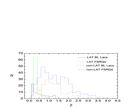
Figure 1: Redshift distributions for BL Lacs detected by Fermi LAT (LAT BL Lacs, black continuous line), FSRQs detected by Fermi LAT (LAT FSRQs, red dashed line), BL Lacs of non $\gamma$-ray loud (non-LAT BL Lacs, green dotted line), FSRQs of non $\gamma$-ray loud (non-LAT FSRQs, blue dot–dashed line).

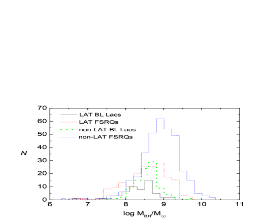
Figure 2: Black hole mass distributions for LAT BL Lacs, LAT FSRQs, non-LAT BL Lacs and non-LAT FSRQs. The meanings of different lines are as same as Fig. 1. The black hole mass distributions for Fermi blazars are $10^{6.5}-10^{9.8}$ ${\rm M_{\rm\odot}}$ and mean value is $10^{8.5\pm 0.03}$ ${\rm M_{\rm\odot}}$; for non-Fermi blazars, the black hole mass distributions are $10^{6.35}-10^{10.24}$ ${\rm M_{\rm\odot}}$ and mean value is $10^{8.82\pm 0.02}$ ${\rm M_{\rm\odot}}$. The mean values for Fermi BL Lacs, Fermi FSRQs, non-Fermi BL Lacs and non-Fermi FSRQs are $10^{8.34\pm 0.06}$ ${\rm M_{\rm\odot}}$, $10^{8.55\pm 0.04}$ ${\rm M_{\rm\odot}}$, $10^{8.54\pm 0.03}$ ${\rm M_{\rm\odot}}$ and $10^{8.9\pm 0.03}$ ${\rm M_{\rm\odot}}$ respectively.

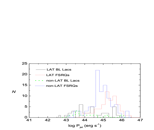
Figure 3: Jet kinetic power distributions for LAT BL Lacs, LAT FSRQs, non-LAT BL Lacs and non-LAT FSRQs. The meanings of different lines are as same as Fig. 1. The jet kinetic power distributions for Fermi blazars are $10^{42.6}-10^{46.5}\rm{erg~{}s^{-1}}$ and mean value is $10^{44.92\pm 0.08}\rm{erg~{}s^{-1}}$; for non-Fermi blazars, the jet kinetic power distributions are $10^{43}-10^{46.4}\rm{erg~{}s^{-1}}$ and mean value is $10^{44.80\pm 0.07}\rm{erg~{}s^{-1}}$. The mean values for Fermi BL Lacs, Fermi FSRQs, non-Fermi BL Lacs and non-Fermi FSRQs are $10^{44.32\pm 0.15}\rm{erg~{}s^{-1}}$, $10^{45.25\pm 0.07}\rm{erg~{}s^{-1}}$, $10^{44.16\pm 0.23}\rm{erg~{}s^{-1}}$ and $10^{44.88\pm 0.06}\rm{erg~{}s^{-1}}$ respectively.

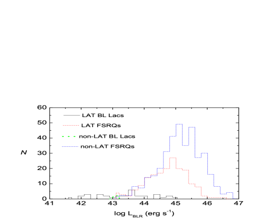
Figure 4: Broad-line luminosity distributions for LAT BL Lacs, LAT FSRQs, non-LAT BL Lacs and non-LAT FSRQs. The meanings of different lines are as same as Fig. 1.

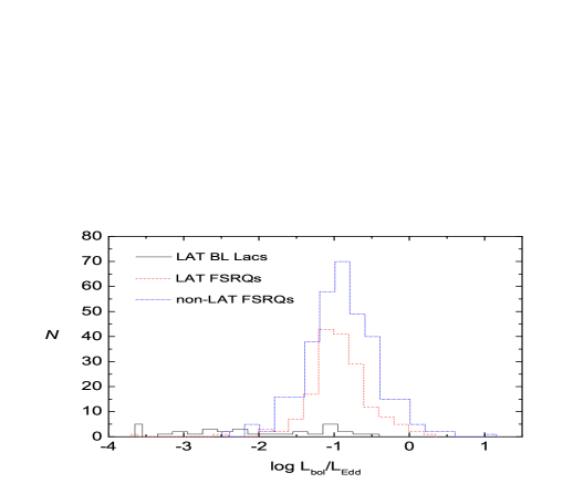
Figure 5: Eddington ratio distributions for LAT BL Lacs, LAT FSRQs and non-LAT FSRQs. The meanings of different lines are as same as Fig. 1.

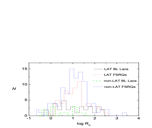
Figure 6: Ratio of the beamed radio core flux density to the unbeamed extended radio flux density distributions for LAT BL Lacs, LAT FSRQs, non-LAT BL Lacs and non-LAT FSRQs. The meanings of different lines are as same as Fig. 1.

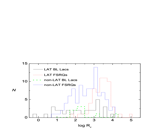
Figure 7: The ratio of the radio core luminosity to the k-corrected absolute V-band magnitude for LAT BL Lacs, LAT FSRQs, non-LAT BL Lacs and non-LAT FSRQs. The meanings of different lines are as same as Fig. 1.

The black hole mass distributions of the various classes are shown in Fig. 2. The black hole mass distributions between all Fermi blazars and all non-Fermi blazars, between Fermi BL Lacs and non-Fermi BL Lacs, between Fermi FSRQs and non-Fermi FSRQs are significant difference ($P<0.0001,P=0.011,P<0.0001$). So we can get that compared with non-Fermi blazars, Fermi blazars have smaller mean black hole mass.

The jet kinetic power distributions of the various classes are shown in Fig. 3. The jet kinetic power distributions between all Fermi blazars and all non-Fermi blazars, between Fermi FSRQs and non-Fermi FSRQs are significant difference ($P=0.01,P=0.0002$). So Fermi blazars have larger mean jet kinetic power than non-Fermi blazars.

The broad-line luminosity distributions of the various classes are shown in Fig. 4. Because non-Fermi BL Lacs almost have not broad-line data, we only compare broad-line luminosity distributions between Fermi FSRQs and non-Fermi FSRQs. The mean values for Fermi FSRQs and non-Fermi FSRQs are $10^{44.72\pm 0.05}\rm{erg~{}s^{-1}}$ and $10^{45.14\pm 0.03}\rm{erg~{}s^{-1}}$ respectively. From KS test, the broad-line luminosity distributions between Fermi FSRQs and non-Fermi FSRQs are significant difference ($P<0.0001$). We also compare the Eddington ratio distributions between Fermi FSRQs and non-Fermi FSRQs (see Fig. 5; $L_{\rm Edd}=1.3\times 10^{38}(\frac{\rm M}{\rm M_{\odot}}){\rm erg~{}s^{-1}},L_{\rm bol}\approx 10L_{\rm BLR}$ from Netzer (1990)). However, the result of KS test shows that they do not have significant difference ($P=0.398$). The mean values for Fermi FSRQs and non-Fermi FSRQs are $10^{-0.93\pm 0.03}$ and $10^{-0.91\pm 0.03}$ respectively.

The distributions for ratio of the beamed radio core flux density to the unbeamed extended radio flux density (core prominence parameter $R_{\rm c}$) are shown in Fig. 6. The $R_{\rm c}$ distributions for Fermi blazars are $10^{-0.3}<R_{\rm c}<10^{2.5}$ and mean value is $10^{1.13\pm 0.07}$; for non-Fermi blazars, the $R_{\rm c}$ distributions are $10^{-0.7}<R_{\rm c}<10^{3.5}$ and mean value is $10^{1.02\pm 0.07}$. The mean values for Fermi BL Lacs, Fermi FSRQs, non-Fermi BL Lacs and non-Fermi FSRQs are $10^{1.09\pm 0.13}$, $10^{1.16\pm 0.07}$, $10^{0.6\pm 0.18}$ and $10^{1.08\pm 0.07}$ respectively. The $R_{c}$ distributions between all Fermi blazars and all non-Fermi blazars, between Fermi BL Lacs and non-Fermi BL Lacs, between Fermi FSRQs and non-Fermi FSRQs are not significant difference ($P=0.4,P=0.26,P=0.85$). Kharb et al. (2010) found that the ratio of the radio core luminosity to the k-corrected optical luminosity ($R_{\rm v}$) appears to be a better indicator of orientation than the traditionally used radio core prominence parameter ($R_{\rm c}$). Wills & Brotherton (1995) defined $R_{\rm v}$ as the ratio of the radio core luminosity to the k-corrected absolute V-band magnitude ($M_{\rm abs}$): $\log R_{\rm v}=\log(L_{\rm core}/L_{\rm opt})=(\log L_{\rm core}+M_{\rm abs}/2.5)-13.7$, where $M_{\rm abs}=M_{\rm v}-k$, and the k-correction is, $k=-2.5\log(1+z)^{1-\alpha_{\rm opt}}$ with the optical spectral index, $\alpha_{\rm opt}=0.5$. Making use of the above Equations, we obtain $R_{\rm v}$ for our sample. The distributions for $R_{\rm v}$ are shown in Fig. 7. The mean values of $R_{\rm v}$ for Fermi blazars and non-Fermi blazars are $10^{2.95\pm 0.1}$ and $10^{2.63\pm 0.07}$ respectively. The $R_{\rm v}$ distribution between all Fermi blazars and all non-Fermi blazars is significant difference ($P=0.001$). Therefore, Fermi blazars have larger mean $R_{\rm v}$ than non-Fermi blazars, which supports that compared with non-Fermi blazars, Fermi blazars are more beamed.

3.2 Black hole mass vs jet power

Figure 8 shows black hole mass as a function of jet power. Different symbols correspond to blazars of different classes. Pearson product-moment analysis (hereafter called Pearson analysis) is applied to analyze the correlations between black hole mass and jet power for all blazars. The results show that the correlations between black hole mass and jet power for both Fermi blazars and non-Fermi blazars are significant (Fermi blazars: number of points $N=91$, significance level $P=3\times 10^{-4}$, coefficient of correlation $r=0.37$; non-Fermi blazars: $N=96$, $P=5\times 10^{-3}$, $r=0.28$).

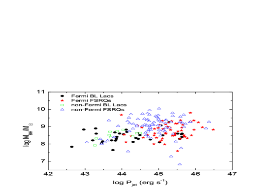
Figure 8: Black hole mass as a function of jet power of various classes. Fermi BL Lacs: black filled circles; Fermi FSRQs: red filled stars; non-Fermi BL Lacs: green empty squares; non-Fermi FSRQs: blue empty triangles. The uncertainties of jet kinetic power and black hole mass are 0.7 dex and 1 dex respectively.

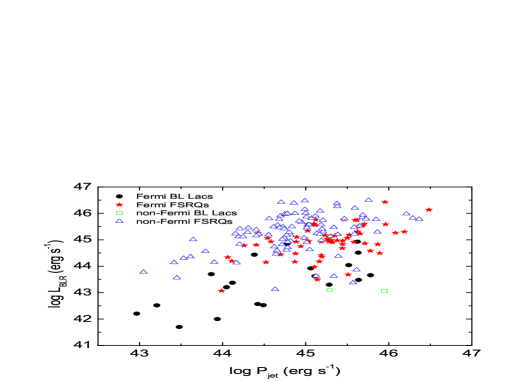
Figure 9: Broad line luminosity as a function of jet power of various classes. The meanings of different symbols are as same as Fig. 8. The uncertainties of jet kinetic power and broad line luminosity are 0.7 dex and 0.5 dex respectively.

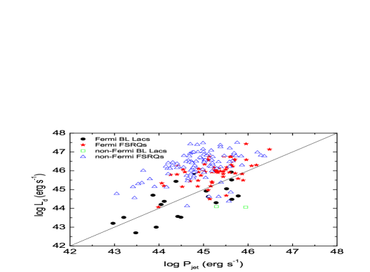
Figure 10: Disk luminosity as a function of jet power of various classes. The black line stands for $P_{\rm jet}=L_{\rm d}$. The meanings of different symbols are as same as Fig. 8. The uncertainties of jet kinetic power and disk luminosity are 0.7 dex and 1 dex respectively.

3.3 Broad line luminosity and disk luminosity vs jet power

Figure 9 shows broad line luminosity as a function of jet power. The results of Pearson analysis show that there are significant correlations between broad line luminosity and jet power for Fermi blazars and non-Fermi blazars ($N=78$, $P=2.6\times 10^{-11}$, $r=0.67$; $N=97$, $P=2\times 10^{-3}$, $r=0.31$). Linear regression is applied to analyze the correlation between broad line luminosity and jet power. And we obtain $\log L_{\rm BLR}\sim(0.94\pm 0.12)logP_{jet}$ for Fermi blazars; $\log L_{BLR}\sim(0.39\pm 0.12)\log P_{\rm jet}$ for non-Fermi blazars (95% confidence level and $r=0.67,0.31$). The Analysis of Variance (ANOVA) is used to test the results of linear regression which shows that it is valid for the results of linear regression (value $F=60.89$, probability $P=2.6\times 10^{-11};F=10.13,P=2\times 10^{-3})$. Figure 10 shows disk luminosity as a function of jet power. From Fig. 10, it is seen that compared with non-Fermi blazars, Fermi blazars are closer to the $P_{\rm jet}=L_{\rm d}$; the jet powers of some BL Lacs are larger than the disk luminosity while some are opposite; the jet power is much smaller than the disk luminosity for most of FSRQs.

We use multiple linear regression analysis to get the relationships between the jet power and both the Eddington luminosity and the broad line region luminosity for Fermi and non-Fermi blazars with 95% confidence level and $r=0.7,0.5$:

$$\log P_{\rm jet}=0.49(\pm 0.06)\log L_{\rm BLR}-0.01(\pm 0.16)\log L_{\rm Edd}+23.6(\pm 7),$$ (2)

$$\log P_{\rm jet}=0.7(\pm 0.14)\log L_{\rm BLR}-0.46(\pm 0.17)\log L_{\rm Edd}+34.71(\pm 4.9).$$ (3)

The ANOVA shows that it is valid for the results of multiple linear regression ($F=33.5,P=5.13\times 10^{-11};F=13.8,P=6.7\times 10^{-6})$. From Equations (2) and (3), we see that for Fermi blazars, the black hole mass does not have significant influence on jet power while for non-Fermi blazars, both accretion disk luminosity (referring to accretion rate; Sbarrato et al. 2014; Ghisellini et al. 2014) and black hole mass have contributions to the jet power.

3.4 The blazar sequence

The $\alpha_{\rm ro}$–$\alpha_{\rm ox}$ plot of our sample is shown in Fig. 11. The $\alpha_{\rm ro}$–$\alpha_{\rm ox}$ plot of BZCAT catalog is given in Fig. 27 of Abdo et al. (2010c). From Fig. 11 of our sample, it is shown that FSRQs are exclusively located along the top-left/bottom-right band; the $\alpha_{\rm ro}$ of most of BL Lacs are located between 0 and 0.8, and 0.8–2 for $\alpha_{\rm ox}$. As a comparison, it is found that the space of $0.5<\alpha_{\rm ox}<0.8$ in Fig. 27 of Abdo et al. (2010c) has some BL Lacs while do not in our Fig. 11; for both our Fig. 11 and Fig. 27 of Abdo et al. (2010c), the top-right space of $\alpha_{\rm ro}$–$\alpha_{\rm ox}$ plot is empty; for the rest of space, our Fig. 11 is consistent with Fig. 27 of Abdo et al. (2010c). Selection effects may cause the deficiency of BL Lacs located in $0.5<\alpha_{\rm ox}<0.8$ in our Fig. 11 because these BL Lacs are more likely to have nothing data about redshift, black hole mass, jet power. Padovani & Giommi (1995) and Abdo et al. (2010c) presented that the $\alpha_{\rm ro}$ of HBL sources are located between 0.2 and 0.4, and 0.9–1.3 for $\alpha_{\rm ox}$. In our sample, this region mainly includes non-Fermi BL Lacs. Compared with non-Fermi FSRQs, Fermi FSRQs are more located in top-left of Fig. 11.

Figure 12 shows synchrotron peak luminosity $L_{\rm peak}$ versus synchrotron peak frequency $\nu_{\rm peak}$ for blazars and Fermi-detected narrow-line Seyfert 1 galaxy. The synchrotron peak luminosity and synchrotron peak frequency for four Fermi-detected narrow-line Seyfert 1 galaxies are collected from Abdo et al. (2009b). Making use of Pearson analysis, we find that there are strong anti-correlations between $L_{\rm peak}$ and $\nu_{\rm peak}$ for all blazars, Fermi blazars and non-Fermi blazars respectively ($r=-0.637,P=4.9\times 10^{-82},N=711$; $r=-0.564,P=1.1\times 10^{-21},N=242$; $r=-0.657,P=3.4\times 10^{-59},N=469$). In Fig. 12, we also find that the four Fermi-detected narrow-line Seyfert 1 galaxies mix in the area of blazars populated, and are in low $\nu_{\rm peak}$–low $L_{\rm peak}$ region, which support that $\gamma$-loud narrow-line Seyfert 1 galaxies have similar mechanisms with blazars, and that the low $\nu_{\rm peak}$–low $L_{\rm peak}$ blazars are more likely to have low black hole mass (see Chen & Bai 2011).

Ghisellini & Tavecchio (2008) extended the shape of SED from a one-parameter (observed bolometric luminosity) to a two-parameter sequence (black hole mass and accretion rate). So in Fig. 13, we give synchrotron peak frequency ($\nu_{\rm peak}$) versus black hole mass and Eddington ratio. From results of Pearson analysis, we get that there is not significant correlation between $\nu_{\rm peak}$ and black hole mass for all blazars ($r=0.03,P=0.38$) while there is significant anti-correlation between $\nu_{\rm peak}$ and Eddington ratio for all blazars ($r=-0.22,P=3.8\times 10^{-7}$).

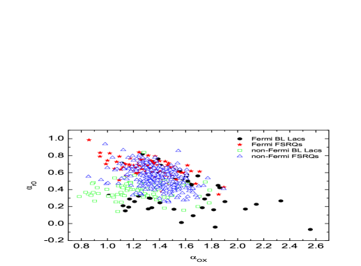
Figure 11: The $\alpha_{\rm ro}$–$\alpha_{\rm ox}$ plot. The meanings of different symbols are as same as Fig. 8.

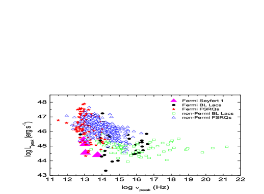
Figure 12: Synchrotron peak luminosity $L_{\rm peak}$ versus synchrotron peak frequency $\nu_{\rm peak}$ for blazars, and Fermi-detected narrow-line Seyfert 1 galaxies. The meanings of different symbols of blazars are as same as Fig. 8. Fermi-detected narrow-line Seyfert 1 galaxies: magenta filled triangles.

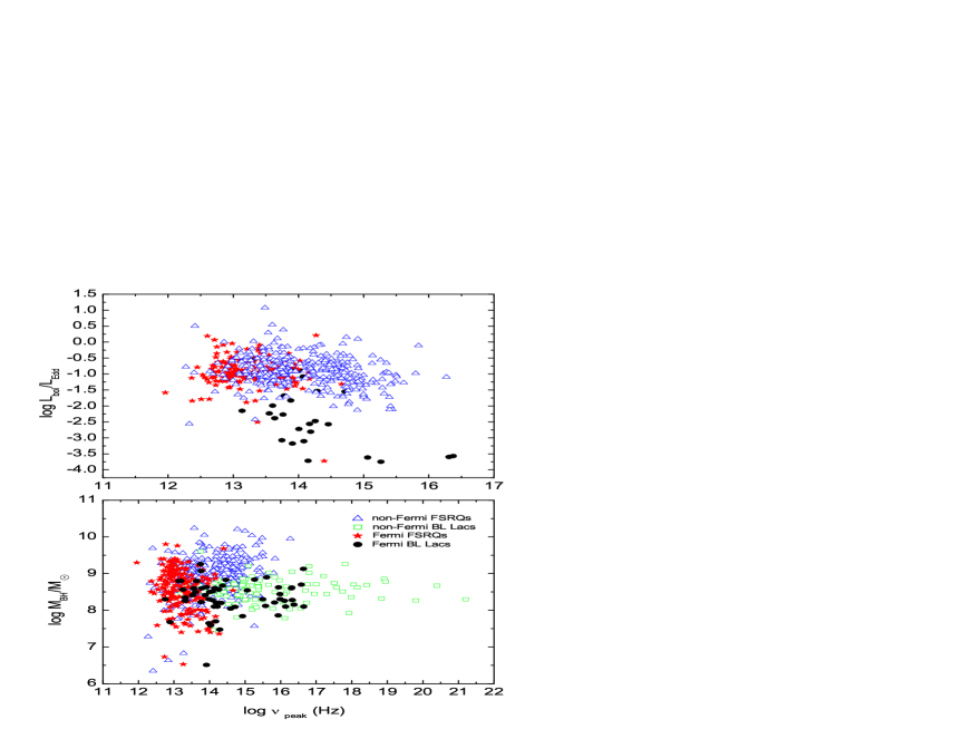
Figure 13: Black hole mass (bottom panel) and Eddington ratio (top panel) versus synchrotron peak frequency ($\nu_{\rm peak}$). The meanings of different symbols of blazars are as same as Fig. 8.

4 Discussions and conclusions

4.1 Possible biases in the evaluations of sample and parameters

For our sample, the selection criteria are: (i) we tried to select the largest group of blazars included in BZCAT with reliable broad line luminosity, redshift, black hole mass and jet kinetic power; (ii) in order to have reliable sample, we did not consider the candidate blazars of unknown type; (iii) the non-Fermi blazars, which were detected by EGRET or recorded in 1LAC but missed in 2LAC, were not included in our sample; (iv) the Fermi blazars only focused on clean 2LAC sample. Based on the above criteria, the following objects can be missed: blazars without measured redshift (mainly including BL Lacs), blazars without measured black hole mass, extended 1.4 GHz radio data and broad line data, blazars of uncertain type (BZU), blazars which were detected by EGRET or recorded in 1LAC but missed in 2LAC and blazars classed into non-clean 2LAC. From our selection criteria of sample, it is shown that the number of BL Lacs is missed more in our sample than that of FSRQs because compared with FSRQs, BL Lacs have much less information about redshift, black hole mass and broad line data. Via comparing our redshift distribution to redshift distribution of complete BZCAT sample, we find that the whole distribution and mean value of redshift from our sample agree with the results of complete BZCAT sample. From complete 2LAC sample (Fig. 12 of Ackermann et al. (2011)), it is shown that the redshift distribution peaks around $z=1$ for FSRQs and extends to $z=3.1$; the redshift distribution for BL Lacs extends to $z=1.5$ and shows a broad maximum between $0.1$ and $0.2$. So through comparing redshift distributions between our Fermi sample (Fig. 1) and complete 2LAC sample, we find that our redshift distribution of Fermi blazars is similar to redshift distribution of complete 2LAC sample. However, this does not necessarily indicate that the distributions of all other quantities are also similar.

In order to reduce the uncertainty, we tried to select the data from a same paper and/or a uniform method. Firstly, for most of FSRQs from our sample (529 FSRQs), black hole masses were estimated by traditional virial method; for most of BL Lacs (150 BL Lacs), the black hole masses can be estimated from the properties of their host galaxies with either $M_{\rm BH}-\sigma$ or $M_{\rm BH}-L$ relations, where $\sigma$ and $L$ are the stellar velocity dispersion and the bulge luminosity of the host galaxies. For a few blazars (29 blazars), the BH masses were estimated from minimum timescale for flux variations ($M_{\rm BH}-\triangle t_{\rm min}$ from Xie et al. (2004)). In our sample, we found that for same blazars, black hole masses estimated from different emission line or different authors had a little difference. For the blazars, when more than one black hole masses were got, we used average BH mass instead. Moreover, we should be caution in the black hole masses estimated from virial method or relations of host galaxies because of non-thermal dominance for blazars and contamination of host galaxy light. Secondly, for calculating the total luminosity of the broad lines, we and the other authors adopted method of Celotti, Padovani & Ghisellini (1997) which scaled several strong emission lines to the quasar template spectrum of Francis et al. (1991). Via comparing broad-line luminosities estimated by us and the other authors, we found that for some blazars, the broad-line luminosities between us and the other authors were slightly different. The possible reasons were that we and the other authors used different lines to calculate broad-line luminosity; variability also can cause the difference of broad-line luminosity. In these blazars, we used average broad-line luminosity instead. It also is worth noting that BLR luminosity is not a direct measure of the disc luminosity and furthermore that it is possible that BL Lacs may have a less luminous accretion disc (radiatively inefficient accretion flow) than FSRQs which would make it difficult to estimate the accretion rate from the BLR or disc luminosity. Thirdly, the jet power of our sample was estimated from extended radio luminosity at 300 MHz. Following Meyer et al. (2011), we extrapolated 1.4 GHz extended radio emission to 300 MHz luminosity, using a low frequency index of $\alpha=1.2$ ($F_{\rm\nu}\propto\nu^{-\alpha}$). It was possible that the extrapolation can bring in uncertainty for estimating jet power. The uncertainty in jet power was dominated by the scatter in the correlation of Cavagnolo et al. (2010). In XZ14, we have compared the jet cavity power to jet power from modeling the SED of Ghisellini et al. (2010), and found that on average, the jet power from Ghisellini et al. (2010) was slightly larger than the jet cavity power. The possible reasons are as follows (Kang et al. 2014; Kharb et al. 2010): (i) when Ghisellini et al. (2010) fitted the SED, they assumed one proton per emitting electron in the jet, whereas the jet power from modeling the SED would be reduced if the jet also included a fraction of $e^{\pm}$ pairs; (ii) the extended radio luminosity is affected by interacting with the environment on kiloparsec-scales. Finally, we discussed $L_{\rm peak}$ and $\nu_{\rm peak}$. At present, fitting simultaneous SED data from long time is an ideal method to determine $L_{\rm peak}$ and $\nu_{\rm peak}$. However, it is hard to obtain simultaneous multi-wave band data for a large sample. For most of our sample, we and Finke (2011) used the empirical relationship of Abdo et al. (2010c) to estimate $\nu_{\rm peak}$. Abdo et al. (2010c) have pointed out that their method assumed that the optical and X-ray fluxes are not contaminated by thermal emission from the disk or accretion. In blazars where thermal flux components are not negligible (this should probably occur more frequently in low radio luminosity sources) the method may lead to a significant overestimation of the position of $\nu_{\rm peak}$. For blazars without X-ray flux, we adopted $\alpha_{\rm ro}$ to estimate $\nu_{\rm peak}$. The $\nu_{\rm peak}$ and $L_{\rm peak}$ of Nieppola et al. (2006) were estimated by fitting non-simultaneous SED data. The $\nu_{\rm peak}$ and $L_{\rm peak}$ of Meyer et al. (2011) were estimated by fitting non-simultaneous average SED. For many blazars, we also used radio luminosity at 5 GHz to estimate the synchrotron peak luminosity. As we know, blazars are high variability. Therefore, the above factors or processes can bring in uncertainties for estimating $\nu_{\rm peak}$ and $L_{\rm peak}$. For $R_{\rm c}$ and $R_{\rm v}$, variability can lead to uncertainties.

4.2 The basic properties of Fermi blazars

By comparing the main parameters between Fermi blazars and non-Fermi blazars, we obtain the below results. (i) The redshift distributions between Fermi blazars and non-Fermi blazars have significant difference. For all blazars and FSRQs, Fermi sources have smaller mean redshift than non-Fermi sources while for only BL Lacs, the result is the opposite. So compared with non-Fermi FSRQs, Fermi FSRQs are relatively nearby objects because the $\gamma$-ray of greater distance object is likely to be absorbed (Piner et al. 2008). But for BL Lacs, the opposite result can be explained as follows. The result of comparison may be a selection effect because based on our sample selection criteria, many BL Lacs are missed. In addition, another possible explanation is that redshift may not be as a main factor for difference between Fermi and non-Fermi BL Lacs, e.g. if the beaming effect is a main reason for difference between Fermi and non-Fermi BL Lacs, a BL Lac with small redshift still can be as a Fermi source as long as it has enough large beaming factor. (ii) The black hole mass distributions between Fermi blazars and non-Fermi blazars have significant difference. Fermi blazars have smaller mean black hole mass than non-Fermi blazars. Generally, one may consider Fermi blazars with a larger black hole mass because a blazar with larger luminosity may have a larger black hole mass (Ghisellini et al. 2010). Our results seem to contradict with the idea. Meier (1999) has demonstrated explicitly that it is not necessary to have a relatively massive black hole mass to produce powerful jet. Based on current accretion and jet production theory (e.g. Blandford & Znajek 1977; Meier 1999), jet power is tied to the spinning of black hole. Then, it is quite possible to have highly powered jet with small black hole mass if the black hole has a high spin (the maximum jet power is close to the Eddington luminosity or an efficiency of $\sim$140% of the accretion power from Tchekhovskoy et al. (2011)). The other possibility is that black hole mass is not main factor for difference between Fermi blazars and non-Fermi blazars. (iii) The jet power distributions between Fermi blazars and non-Fermi blazars have significant difference. Fermi blazars have larger mean jet power than non-Fermi blazars. In our sample, the jet power estimated requires assumption about the energy required to inflate the lobe, and is free of beaming effect because our jet power is estimated from extended radio emission. So the result supports that Fermi blazars are likely to have a more powerful jet. (iv) The Eddington ratio distributions between Fermi FSRQs and non-Fermi FSRQs do not have significant difference, which does not mean that the accretion rate distributions between them also are similar. The fact that similar Eddington ratio distributions between them means similar accretion rate distributions is only implied if the black hole masses are also very similar. The broad-line luminosity distributions between Fermi FSRQs and non-Fermi FSRQs have significant difference. Compared with non-Fermi FSRQs, Fermi FSRQs have smaller mean broad-line luminosity. Theoretically, the continuum flux is believed to be responsible for ionizing the cloud material in the broad line region (e.g. Arshakian et al. 2010). So compared with non-Fermi blazars, Fermi blazars may have larger broad line luminosity because Fermi blazars have larger jet power than non-Fermi blazars. But this is opposite with our results. A probable explanation is that broad-line luminosity is not main factor for difference between Fermi blazars and non-Fermi blazars, e.g. a blazar with low broad line luminosity still can be as Fermi source as long as it has enough large beaming factor. Moreover, it is possible due to redshift distribution effect: Fermi FSRQs have smaller mean redshift than non-Fermi FSRQs, and increasing average redshift may cause increasing line luminosity (see Ghisellini & Tavecchio 2015). (v) The $R_{\rm c}$ can be as indicators of Doppler beaming and orientation. From our sample, we find that the mean difference between $R_{\rm c}$ for Fermi and non-Fermi blazars is small and not significant. Kharb et al. (2010) found that the $R_{\rm v}$ appears to be a better indicator of orientation than the traditionally used $R_{\rm c}$, since the optical luminosity is likely to be a better measure of intrinsic jet power (e.g. Maraschi et al. 2008; Ghisellini et al. 2009c) than extended radio luminosity. This is due to the fact that the optical continuum luminosity is correlated with the emission-line luminosity over four orders of magnitude (Yee & Oke 1978), and the emission-line luminosity is tightly correlated with the total jet kinetic power (Rawlings & Saunders 1991). The extended radio luminosity, on the other hand, is suggested to be affected by interaction with the environment on kiloparsec-scales. Our comparing results show that the $R_{\rm v}$ distributions between Fermi blazars and non-Fermi blazars are significant difference and that the mean value of $R_{\rm v}$ for Fermi blazars is larger than that for non-Fermi blazars. Therefore, our results provide new supports for that compared with non-Fermi blazars, Fermi blazars have a stronger beaming effect.

The jet formation remains one of the unsolved fundamental problems in astrophysics (e.g. Meier, Koide & Uchida 2001). Many models have been proposed to explain the origin of jets. In current theoretical models of the formation of jet, power is generated via accreting material and extraction of rotational energy of disc/black hole (Blandford & Znajek 1977; Blandford & Payne 1982), and then converted into the kinetic power of the jet. Our results show that the correlations between black hole mass and jet power for both Fermi and non-Fermi blazars are significant. The results of Pearson analysis show that there are significant correlations between broad line luminosity and jet power for both Fermi blazars and non-Fermi blazars, which supports that the jet power has a close link with accretion rate (Sbarrato et al. 2014; Ghisellini et al. 2014). The result is consistent with other authors (e.g. Rawlings & Saunders 1991; Falcke & Biermann 1995; Serjeant, Rawlings & Maddox 1998; Cao & Jiang 1999; Wang, Luo & Ho 2004; Liu, Jiang & Gu 2006; Xie et al. 2007; Ghisellini, Tavecchio & Ghirlanda 2009a; Ghisellini et al. 2009b, 2010, 2011; Gu, Cao & Jiang 2009; Sbarrato et al. 2012). Linear regression is applied to analyze the correlation between broad line luminosity and jet power, and we obtain $\log L_{\rm BLR}\sim(0.94\pm 0.12)\log P_{\rm jet}$ for Fermi blazars and $\log L_{\rm BLR}\sim(0.39\pm 0.12)\log P_{\rm jet}$ for non-Fermi blazars. In addition, from Equations (2) and (3), we find that for Fermi blazars, the black hole mass does not have significant influence on jet power while for non-Fermi blazars, both accretion disk luminosity (or accretion rate) and black hole mass have contributions to the jet power. These also can explain our result that the distributions of jet power between Fermi and non-Fermi blazars are significant difference.

4.3 The blazar sequence

From Fig. 12 and making use of Pearson analysis, we find that there are strong anti-correlations between $L_{\rm peak}$ and $\nu_{\rm peak}$ for all blazars, Fermi blazars and non-Fermi blazars respectively. The results support the “blazar sequence” and are not same with results of Meyer et al. (2011). In Fig. 4 of Meyer et al. (2011), an “L”-shape in the $L_{\rm peak}$–$\nu_{\rm peak}$ plot seems to have emerged which destroys the “blazar sequence”. However, the “L”-shape in Meyer et al. (2011) may be a selection effect of sample. A very possible reason is that in $10^{14}{\rm Hz}<\nu_{\rm peak}<10^{15}{\rm Hz}$ interval of $L_{\rm peak}$–$\nu_{\rm peak}$ plot of Meyer et al. (2011), there are few blazars. If the interval is full of some blazars, then the “L”-shape will be weaken or disappeared. In our Fig. 12, the interval has many blazars which fill in the interval of Fig. 4 of Meyer et al. (2011). And the result is consistent with others. From Fig. 2 of Nieppola et al. (2008) and Fig. 2, 5 of Finke (2013), it was seen that their the interval still has some blazars. Giommi et al. (2012) used extensive Monte Carlo simulations to get the relation plot of $\nu_{\rm peak}-L_{\rm 5GHz}$ which shows that the interval still has many blazars. The Compton dominance, the ratio of the peak of the Compton to the synchrotron peak luminosities, is essentially a redshift-independent quantity. Finke (2013) used Compton dominance to study the “blazar sequence”. The results of Finke (2013) showed that a correlation exists between Compton dominance and the peak frequency of the synchrotron component for all blazars, including ones with unknown redshift. The sample of Finke (2013) is the 2LAC clean sample. The $\gamma$-ray flares in blazars are likely to occur when the sources are in the high state (Fan et al. 1998). If this is true, the blazars from Finke (2013) are likely to stand for active states of the sources, not their necessarily averaged status. Finke (2013) also presented that SSC emission has the same beaming pattern as synchrotron, and thus Compton dominance does not depend on the viewing angle; however, EC emission does not have the same beaming pattern as synchrotron and SSC, and so Compton dominance is dependent on the viewing angle. Piner & Edwards (2013) have found that beaming factors in the $\gamma$-ray and radio bands are different yet correlated for TeV blazars. An obvious explanation for the ‘bulk Lorentz factor crisis’ is that the radio and $\gamma$-ray emissions are produced in different parts of the jet with different bulk Lorentz factors (Henri & Sauge 2006; Piner, Pant & Edwards 2008, 2010; Piner & Edwards 2013). Therefore, it is possible that the correlation between Compton dominance and peak frequency of the synchrotron component can be resulted from beaming effect. For our Fig. 12, if high $\nu_{\rm peak}$ high $L_{\rm peak}$ blazars are included, the correlation of $\nu_{\rm peak}-L_{\rm peak}$ will be destroyed. The results of Giommi et al. (2012) also showed that the phenomenological “blazar sequence” is a selection effect. Nieppola et al. (2008) proposed that after being Doppler-corrected, the anti-correlation between $\nu_{\rm peak}$ and $L_{\rm peak}$ become positive correlation. However, due to limit of Doppler factor, we can not determine the effects of beaming on the blazar sequence in this paper. Ghisellini & Tavecchio (2008) revisited the blazar sequence and proposed that the power of the jet and SED of its emission are linked to the mass of black hole and the accretion rate. From results of Pearson analysis, we get that there is not significant correlation between synchrotron peak frequency and black hole mass for all blazars while significant anti-correlation between synchrotron peak frequency and Eddington ratio for all blazars. The scatter in $\nu_{\rm peak}-L_{\rm bol}/L_{\rm Edd}$ plot can be resulted from uncertainties of $\nu_{\rm peak}$ and black hole mass.

Table 1: The non-Fermi sample.

BZCAT name	Other name	RA	Redshift	$\log\nu_{\rm peak}$	$\log P_{\rm jet}$	$\log M_{\rm BH}$	$\log L_{\rm BLR}$	$\log R_{\rm c}$
		DEC		$\log L_{\rm peak}$		ref	ref	ref
(1)	(2)	(3)	(4)	(5)	(6)	(7)	(8)	(9)
BZQ J0006-0623	0003-066	00 06 13.9	0.347	13.16†	44.63		43.13	1.48
		-06 23 35		46.22†			C99	C07
BZQ J0010+1058	0007+106	00 10 31.0	0.089	14.88	43.41	8.29	44.14	0.62
		+10 58 30		45.05		C12	C12	K10
BZQ J0017+8135	0014+813	00 17 08.5	3.366	14.55†			46.62
		+81 35 08		46.99			C99
BZQ J0019+7327	0016+731	00 19 45.8	1.781	13.26†	45.19	8.93	44.98	1.27
		+73 27 30		47.65†		C12	C12	K10
BZB J0022+0006	SDSS J002200.95+000657.9	00 22 00.9	0.306	16.17		8.49
		+00 06 58		44.28		P11
BZQ J0038+4137	0035+413	00 38 24.8	1.353	13.20		8.53	44.64
		+41 37 06		46.75		C12	C12
BZB J0056-0936	SDSS J005620.07-093629.7	00 56 20.1	0.103	15.01		8.89,8.39
		-09 36 30		44.82		L11
BZQ J0057-0024	SDSS J005716.99-002433.2	00 57 17.0	2.752	13.99		9.73	45.68
		-00 24 33		46.62		S11	S11
BZQ J0059+0006	0056-001	00 59 05.5	0.719	13.58		8.71,8.37,9.03,8.86	44.91
		+00 06 52		46.49		W02,L06,S11	L06
BZB J0110+4149	NPM1G +41.0022	01 10 04.8	0.096	17.74†		8.51
		+41 49 51		44.05†		W09
BZQ J0115-0127	0112-017	01 15 17.1	1.365	13.54		7.85	45.26
		-01 27 05		46.85		C12	C12
BZQ J0121+1149	0119+115	01 21 41.6	0.57	12.81	45.12		43.63	0.84
		+11 49 50		46.29			C99	K10

(a) References. A85: Antonucci & Ulvestad (1985); Ca99: Cassaro et al. (1999); C12: Chai et al. (2012); C07: Cooper et al. (2007); C04: Caccianiga & Marcha (2004); C99: Cao & Jiang (1999); F03: Falomo et al. (2003); K10: Kharb et al. (2010); L08: Landt & Bignall (2008); L06: Liu et al. (2006); L11: Leon-Tavares et al. (2011); M93: Murphy et al. (1993); P11: Plotkin et al. (2011); S11: Shen et al. (2011); W09: Wu et al. (2009); W05: Woo et al. (2005); W04: Wang et al. (2004); W02: Woo & Urry (2002); W00: White et al. (2000).

(b) For $\log\nu_{\rm peak}$ and $\log L_{\rm peak}$, values with a “ $\dagger$ ” represent that they are directly from references.

(c) This table is published in its entirety in the electronic edition. A portion is shown here for guidance.

References

- Aatrokoski et al. (2011) Aatrokoski J. et al., 2011, A&A, 536, A15
- Abdo et al. (2009) Abdo A.A., Ackermann M., Ajello M. et al., 2009a, ApJ, 700, 597
- Abdo et al. (2009) Abdo A.A. et al., 2009b, 707, L142
- Abdo et al. (2010a) Abdo A.A., Ackermann M., Ajello M. et al., 2010a, ApJS, 188, 405
- Abdo et al. (2010b) Abdo A.A., Ackermann M., Ajello M. et al., 2010b, ApJ, 715, 429
- Abdo et al. (2010c) Abdo A.A., Ackermann M., Agudo I. et al., 2010c, ApJ, 716, 30
- Abdo et al. (2012) Abdo A.A., Ackermann M., Ajello M. et al., 2012, ApJS, 199, 31
- Ackermann et al. (2011a) Ackermann M., Ajello M., Allafort A. et al., 2011, ApJ, 743, 171
- Angel (1980) Angel J.R.P. & Stockman H.S., 1980, ARA&A, 18, 321
- Antonucci (1985) Antonucci R.R.J. & Ulvestad J.S., 1985, ApJ, 294, 158
- Arshakian (2010) Arshakian T.G., Leon-Tavares J., Lobanov A.P., Chavushyan V.H., Shapovalova A.I., Burenkov A.N. & Zensus J.A., 2010, MNRAS, 401, 1231
- Balmaverde et al. (2008) Blandford R.D. & Znajek R.L., 1977, MNRAS, 179, 433
- Balmaverde et al. (2008) Blandford R.D. & Payne D.G., 1982, MNRAS, 199, 883
- Caccianiga (2004) Caccianiga A. & Marcha M.J.M., 2004, MNRAS, 348, 937
- Cassaro (1999) Cassaro P. et al., 1999, A&AS, 139, 601
- Cavagnolo (2010) Cavagnolo K.W. et al., 2010, ApJ, 720, 1066
- Cavaliere & D’Elia (2002) Cavaliere A. & D’Elia V., 2002, ApJ, 571, 226
- Cao & Jiang (1999) Cao X. & Jiang D.R., 1999, MNRAS, 307, 802
- Celotti et al. (1997) Celotti A., Padovani P. & Ghisellini G., 1997, MNRAS, 286, 415
- Chai et al. (2012) Chai B., Cao X. & Gu M., 2012, ApJ, 759, 114
- Chen et al. (2011) Chen L. & Bai J.M., 2011, ApJ, 735, 108
- Cheng & Zhang (2000) Cheng K.S., Zhang X. & Zhang L., 2000, ApJ, 537, 80
- Cooper (2007) Cooper N.J., Lister M.L. & Kochanczyk M.D., 2007, ApJS, 171, 376
- Falcke & Biermann (1995) Falcke H. & Biermann P.L., 1995, A&A, 293, 665
- Falomo (2003) Falomo R., Kotilainen J.K., Carangelo N. & Treves A., 2003, ApJ, 595, 624
- Fan (1998) Fan J.H. et al., 1998, A&A, 338, 27
- Finke (1994) Finke J.D., 2013, ApJ, 763, 134
- Fossati et al. (1998) Fossati G., Maraschi L., Celotti A. et al., 1998, MNRAS, 299, 433
- Francis et al. (1991) Francis P.J., Hewett P.C., Foltz C.B., Chaffee F.H., Weymann R.J. & Morris S.L., 1991, ApJ, 373, 465
- Francis et al. (1991) Georganopoulos M., Kirk J.G. & Mastichiadis A., 2001, in ASP Conf. Ser. 227, Blazar Demographics and Physics, ed. P. Padovani & C. Megan Urry (San Francisco, CA: ASP), 116
- Ghisellini (1998) Ghisellini G., Celotti A., Fossati G. et al., 1998, MNRAS, 301, 451