Influence of magnetic surface anisotropy on spin wave reflection from the edge of ferromagnetic film

Abstract

We study propagation of the Gaussian beam of spin waves and its reflection from the edge of thin yttrium-iron-garnet film with in-plane magnetization perpendicular to this edge. We have performed micromagnetic simulations supported by analytical calculations to investigate the influence of the surface magnetic anisotropy present at the film edge on the reflection, especially in the context of the Goos-Hänchen effect. We have shown the appearance of a negative lateral shift between reflected and incident spin wave beams’ spots. This shift is particularly sensitive to the surface magnetic anisotropy value and is a result of the Goos-Hänchen shift which is sensitive to the magnitude of the anisotropy and of the bending of the spin wave beam. We have demonstrated that the demagnetizing field provide graded increase of the refractive index for spin waves, which is responsible for the bending.

In recent years magnetic nanostructures with controlled magnetization dynamics have been considered as candidates for design of new miniaturized devices with enhanced performance and functionality for various applications, e.g. heat transport, energy conversion, magnetic field sensing, information storage and processing.(Shibata04, ; Kajiwara13, ; Stamps14, ) Spin waves (SWs), being propagating collective excitations of the magnetization are also regarded as information carriers, which can be exploited for information processing in devices potentially competitive with standard CMOS systems.(Krawczyk14, ; Chumak14, ) Thus, understanding of SW properties in nanostructures is crucial in designing magnonic units and this is one of the main goal in the research field called magnonics.(Kruglyak10, ; Demokritov13, ) It is expected that magnonic devices allow energy-efficient processing of information which will combine the advantages of photonics (high frequency and wide band) and electronics (miniaturization) in a single unit.(Khitun12, ) One of the basic phenomena connected with wave propagation is the wave transmission and reflection.(Kostylev07, ; Chumak09, ; Dvornik11, ) The reflection of SWs is determined by magnetic properties of the film and boundary conditions at the border of the ferromagnetic material. The reflection of SWs has already been investigated in theoretical and experimental papers(Chumak09, ; Kim08, ) where SWs were treated as plane waves. Use of wave beams, instead of the plane waves or spherical waves, in many cases, can be much more useful and opens new possibilities due to its coherence and low divergence. The known example of the wave beam is a light beam emitted by laser. Usually, its intensity profiles can be described by Gaussian distribution (beams with such property are called Gaussian beams). However, in magnonics the idea of SW beams is unexplored, with only a few theoretical and experimental studies considering formation of SW beams at low frequencies due to the caustic or nonlinear effects.(Vugal88, ; Floyd84, ; Schneider10, ; Gieniusz13, ; Kostylev11, ; Boyle96, ; Bauer97, )

An interesting phenomenon characteristic for the reflection of beam is a possibility for occurrence of a lateral shift of the beam spot along the interface between the reflected and the incident beams - this phenomenon is called as the Goos-Haenchen (GH) effect. The GH effect was observed for electromagnetic waves,(Goos47, ) acoustic waves,(Declercq08, ) electrons (Sharma11, ) and neutron waves.(deHaan10, ) Also for SWs this topic was investigated theoretically for the reflection of the exchange SWs (i.e., high frequency SWs with neglected dipole-dipole interactions) from the interface between two semi-infinite ferromagnetic films.(Dadoenkova12, ) It was shown that for the observation of the GH shift an interlayer exchange coupling between materials is crucial. Recently, we analyzed the GH shift at reflection of the SW’s beam from the edge of the magnetic metallic (Cobalt and Permalloy) and magnetic dielectric yttrium-iron-garnet (YIG, $\mathrm{Y_{3}Fe_{5}O_{12}}$) films.(Gruszecki14, ) We showed that the GH effect exists for dipole-exchange spin waves and can be observed experimentally. The magnetic properties at the film edge were shown to be crucial for a shift of the SW’s beam.

In this paper we analyze the SW beam reflected from the edge of the thin ferromagnetic film. We focus our study on the magnetic properties of the film’s edge and its contribution to the shift of the SW beam. We show, that measurements of this shift can provide information about the local values of the surface magnetic anisotropy, and thus also about the local magnetic properties at the edges of the magnetic film. Our attention is concentrated on detailed investigation of the SW reflection from the YIG film, a dielectric magnetic material highly suitable for magnonic applications due to its low SW damping, which is the smallest among all known magnetic materials.(Serga12, ) Recent experiments have shown possibility of fabrication of very thin YIG films (with thicknesses down to tens of nm(Sun12, ; Sun13, )), which can be patterned on nanoscale and in which the SW dynamics can be controlled with metallic capping layers.(Liu14, ; Pirro14, ) The magnetic properties of the film edge influence SW dynamics, their significance increases with decreasing size of device and will play important role in spintronic and magnonic nanoscale devices.(Shaw08, ; Putter09, ; Ozatay08, ; Xiao12, ; daSilva13, ) However, edge properties at this scale are hardly accessible to experimental techniques. In this paper, we propose a tool for the investigation of the magnetic properties at the edges of thin ferromagnetic film, which exploits shift of SW beams’ spot at the reflection.

The micromagnetic simulations (MMS) and the analytical model of the GH shift are described in section I. Comparison of the results emerging from the analytical model with MMS, development of the model of SW bending and the discussion of the results are presented in section II. The paper is summarized in section III.

I Model and methods

I.1 Model

We consider a thin YIG film with the thickness, $L_{z}=5$ nm, much smaller than lateral dimensions of the film ($L_{z}\ll L_{x},L_{y}$) as it is shown in figure 1. The film is magnetically saturated by an in-plane static external magnetic field $\mathbf{H}$ (we assume a value $\mu_{0}H=0.7$ T) which is applied along the $y$-axis, perpendicular to the edge of the film. We study SWs which propagate in the film plane ($x,y$). The considered edge of the film is along $x$ axis and located at $y=0$. For description of the SW propagation, it is more convenient to define also the second coordinate system ($x^{\prime},y^{\prime}$). As it is shown in Fig. 1, in this coordinate system the wave vector $\mathbf{k_{\mathrm{i}}}$ of the incident SW is parallel to $y^{\prime}$ axis and wave fronts are parallel to $x^{\prime}$ axis. Therefore, we can define the angle of incidence $\theta_{\mathrm{i}}$ as the angle spanned between $\mathbf{k_{\mathrm{i}}}$ and normal to the edge ($y$ axis). We limit angle of incidence to the value $\theta_{\mathrm{i}}=60^{\circ}$ in this study. We assume the SW frequency $f=35$ GHz, at this frequency the propagation is almost isotropic in the film plane due to significant contribution of the exchange interactions (as confirmed latter in the paper with calculated isofrequency contours). In calculations we have used magnetic parameters for YIG at low temperatures: saturation magnetization $M_{\mathrm{S}}=0.194\times 10^{6}$ A/m and exchange constant $A=0.4\times 10^{-11}$ J/m. An additional advantage of the YIG film is its relatively small static demagnetizing field, which is proportional to $M_{\mathrm{S}}$. All these properties of YIG simplify the analysis and helps us to focus mainly on the influence of the surface magnetic anisotropy on the reflection of SWs. The surface magnetic anisotropy can have different origin, besides change of the crystallographic structure at the edge, the applying coating material and roughness can also influence surface anisotropy.(Yen79, ; Bruno89, ; Gradmann86, ; Johnson96, ; Jamet04, ) Nonetheless, the microscopic mechanism of surface magnetic anisotropy is not the subject of this paper, our main concern is the influence of anisotropy on the reflection of a SW beam.

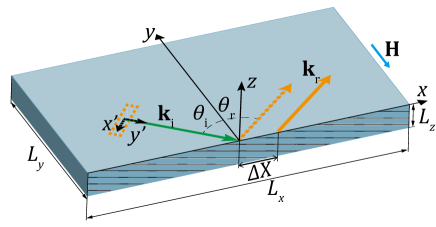
Figure 1: Schematic plot of the thin YIG film geometry considered in the paper. The film has thickness $L_{z}$, which is much smaller than the film’s lateral sizes, $L_{x}$ and $L_{y}$. The ($x,y,z$) coordinating system defines the structure with the film edge at $y=0$ (hatched area). The coordinating system ($x^{\prime},y^{\prime},z$) defines the SW beam, with the wave vector parallel to $y^{\prime}$ and wave fronts parallel to $x^{\prime}$. The area hatched by orange lines and located in the center of coordinate system ($x^{\prime},y^{\prime},z$) corresponds to the excitation area. $\mathbf{k_{\mathrm{i}}}$ and $\mathbf{k_{\mathrm{r}}}$ are wavevectors of incident and reflected SW beams, respectively. $\Delta X$ is a total shift of the SW beam reflected at the edge.

Magnetization dynamics is described by the Landau-Lifshitz (LL) equation of motion for the magnetization vector $\mathbf{M}$:

$$\frac{\mathrm{d}\mathbf{M}}{\mathrm{d}t}=-\frac{\left|\gamma\right|}{1+\alpha^{2}}\mathbf{M}\times\mathbf{H}_{\mathrm{eff}}-\frac{\alpha\left|\gamma\right|}{M_{\mathrm{S}}\left(1+\alpha^{2}\right)}\mathbf{M}\times\left(\mathbf{M}\times\mathbf{H}_{\mathrm{eff}}\right),$$ (1)

where: $\alpha$ - is the damping parameter, $\gamma$ - the gyromagnetic ratio, $\mathbf{H}_{\mathrm{eff}}$ - effective magnetic field. The first term in the LL equation describes precessional motion of the magnetization around the effective magnetic field and the second term enriches that precession by damping. The effective magnetic field in general can consist of many terms. In this paper we consider only the most important contributions: the external magnetic field $\mathbf{H}$, the non-uniform exchange field $\mathbf{H}_{\mathrm{ex}}$ and the long-range dipolar field $\mathbf{H}_{\mathrm{d}}$: $\mathbf{H}_{\mathrm{eff}}=\mathbf{H}+\mathbf{H}_{\mathrm{ex}}+\mathbf{H}_{\mathrm{d}}$.

I.2 Analytical model of the GH shift

In our analytical study we consider SWs with large wavevectors, where the contribution from the dynamic dipole interactions is small and SW dynamics is mainly determined by the exchange interactions. In Eq. (1) we will also make a linear approximation, which allows us to decompose the magnetization vector into a static part equal to the saturation magnetization ${\mathbf{M}}_{\mathrm{S}}$ and a dynamical part laying in the plane perpendicular to the direction of ${\mathbf{M}}_{\mathrm{S}}$: $\mathbf{M}=-M_{\mathrm{S}}\hat{\mathbf{y}}+\mathbf{m}\left(x,y,t\right)$. This approximation is valid when the dynamical part of the magnetization, $|\mathbf{m}|$ is much smaller than the saturation magnetization $M_{\mathrm{S}}$. With this approximation we can assume harmonic time dependency for $\mathbf{m}\propto e^{\mathrm{i}\omega t}$, where $\omega$ is the angular frequency of SW. SWs’ damping is neglected here. To study the incidence and reflection of SWs from the edge of the thin film, we start with dispersion relation for SWs in thin film assuming that the wave vector is in plane of the film:(Kalinikos86, )

$$\omega^{2} = \left[\omega_{\mathrm{H}}+l_{\mathrm{ex}}^{2}\omega_{\mathrm{M}}k^{2}+\omega_{\mathrm{M}}\left(1-f\left(kL\right)\right)\right]\times$$ (2)

$$\left[\omega_{\mathrm{H}}+l_{\mathrm{ex}}^{2}\omega_{\mathrm{M}}k^{2}+\omega_{\mathrm{M}}f\left(kL\right)\sin^{2}\theta_{\mathbf{k}}\right],$$

where: $\mu_{0}$ is permeability of vacuum, $\omega_{\mathrm{H}}=\left|\gamma\right|\mu_{0}H_{\mathrm{i}}$, is the internal field, for the in-plane magnetic field we assume $H_{\mathrm{i}}=H$ , $\omega_{\mathrm{M}}=\gamma\mu_{0}M_{\mathrm{S}}$, and the exchange length $l_{\mathrm{ex}}=\sqrt{2A/(\mu_{0}M_{\mathrm{S}}^{2})}$, $k$ is a wave number, $\theta_{\mathbf{k}}$ is the angle between the saturation magnetization and the in-plane wave vector ${\bf{k}}$, and

$$f\left(x\right)=1-\frac{\left(1-\text{e}^{-x}\right)}{x}.$$ (3)

We assume that the wave number is large, i.e., the condition $kL_{z}\gg 1$ is satisfied. Therefore, the SW dispersion relation can be simplified ($\theta_{\mathbf{k}}=\theta_{\mathrm{i}}$ in our geometry, see Fig. 1) and reduced to the well-known Herring-Kittel equation:

$$\omega^{2}=\left(\omega_{\mathrm{H}}+l_{\mathrm{ex}}^{2}\omega_{\mathrm{M}}k^{2}\right)\left(\omega_{\mathrm{H}}+l_{\mathrm{ex}}^{2}\omega_{\mathrm{M}}k^{2}+\omega_{\mathrm{M}}\sin^{2}\theta_{\mathrm{i}}\right),$$ (4)

For further calculations we need formula for $k$ as a explicit function of the frequency $\omega$. This dependence takes the following form:

$$k^{2}=\frac{\mu_{0}M_{\mathrm{S}}}{4A}\left(-2H-M_{\mathrm{S}}\sin^{2}\theta_{\mathrm{i}}+\sqrt{\frac{4\omega^{2}}{\mu_{0}^{2}\gamma^{2}}+M_{\mathrm{S}}^{2}\sin^{4}\theta_{\mathrm{i}}}\right).$$ (5)

The calculation of the reflection coefficient requires the introduction of the boundary conditions at the film edge (at $y=0$) for $\mathbf{m}$. We show below that the magnetization vector $\mathbf{m}$ components of the SW at the film edge (plane $y=0$) satisfy the following boundary conditions of the Rado-Weertman type:(Rado59, )

$$\left[\frac{\partial\mathbf{m}\left(y\right)}{\partial y}+d\mathbf{m}\left(y\right)\right]_{y=0}=0$$ (6)

where $d$ is an effective pinning parameter. This pinning parameter can take into account the dipole contribution in the finite width stripe ($L_{y}$ is finite) and also contributions from the exchange interaction and a surface magnetic anisotropy at the edge of the film. The former contribution is anisotropic in restricted geometry and have to be calculated in our particular case. To do that we start from the boundary conditions written in the paper Ref. [Guslienko05, ] (see Eq. (2) there):

$$\mathbf{M}\times\left(l_{\text{ex}}^{2}\frac{\partial\mathbf{M}}{\partial\mathrm{n}}-\frac{1}{\mu_{0}}\nabla_{\mathbf{M}}E_{\text{a}}+{\mathbf{H}}_{\text{d}}L_{z}\right)=0$$ (7)

is the energy density of the uniaxial surface anisotropy, $\mathbf{n}$ is the unit vector along the anisotropy axis, $K_{\mathrm{s}}$ is a surface anisotropy constant, and $\mathbf{H}_{\text{d}}$ is the inhomogeneous magnetostatic field near the surface. The authors of the papers [Gus02, ; Guslienko05, ] assumed that the static magnetization is parallel to the magnetic element surface and deduced the pinning of the dynamic magnetization component directed perpendicularly to the surface. Such perpendicular magnetization component corresponds to increasing of the surface magnetostatic energy, which is an effective easy plane surface anisotropy. An additional uniaxial surface anisotropy can be accounted leading to a re-normalization of the magnetostatic anisotropy. The system tries to reduce the surface magnetic charges developing some inhomogeneous magnetization configuration near the surface. But this costs an additional volume magnetostatic and exchange energy. The pinning was strong for thin ($L_{z}$ = 2–20 nm) magnetic elements reflecting a balance between these energy contributions. The pinning calculated in Refs. [Gus02, ; Guslienko05, ] is a result of rapid change of the dynamic magnetostatic field near the surface (on distance about of $L_{z}$). Whereas, in our case the static magnetization is perpendicular to the surface (film edge, the plane $y=0$) and the dynamical magnetization components are parallel to the surface plane $xOz$. Moreover, there is a SW wave vector component $k_{x}$ parallel to the surface. The pinning also has magnetostatic contribution due to the strong dependence of the static dipolar field $H_{\text{d}}\left(y\right)$ on the $y$-coordinate near the surface plane $y=0$. This dipolar pinning competes with the pinning induced by the surface anisotropy. Therefore, the contribution of even weak surface anisotropy is important in this case. We can re-write the boundary condition equations in the symmetric explicit form:

$$\frac{l_{\text{ex}}^{2}}{L_{z}}\frac{\partial{\mathbf{m}}}{\partial{n}}+{\mathbf{h}}+\left[\frac{1}{2}-\frac{\kappa_{\text{s}}}{L_{z}}\right]{\mathbf{m}}=0,$$ (8)

where $\kappa_{\text{s}}=2K_{\text{s}}/\mu_{0}M_{\text{S}}^{2}$, $\mathbf{H}_{\text{d}}=\mathbf{H}_{\text{d}}^{o}+\mathbf{h}$ and the contributions from exchange, dynamical dipolar, static dipolar, and surface anisotropy fields, respectively, are included. The magnetization precession in such non-ellipsoidal element under consideration (see Fig. 1) is elliptical due to non-equivalent dynamical dipolar field components $h_{x}$ and $h_{z}$ along the film normal $Oz$ and in-plane $Ox$ directions.

The dipolar field components can be expressed via the dynamical magnetization components using the method of the tensorial magnetostatic Green functions, see Appendix A and Ref. [Gus11, ]. Even assuming that the dynamical magnetization does not depend on the thickness coordinate $z$ and averaging over $z$ we still have two-dimensional problem because the magnetization depends on the in-plane coordinates $x,y$. We assume that the dynamical magnetization can be represented in the form $m_{\alpha}\left(x,y\right)=\text{exp}\left(ik_{x}x\right)m_{\alpha}\left(y\right)$, where $k_{x}$ is almost continuous variable due to large element size along $Ox$ direction. The magnetization profile $m_{\alpha}\left(y\right)$ can deviate from the plane wave near the element edge, where dipolar fields are strongly inhomogeneous. Using the Green functions formalism we simplify the boundary conditions given by Eq. (8) and write them in the generalized Rado-Weertman form:

$$\left[\frac{\partial m_{\alpha}}{\partial y}+d_{\alpha}m_{\alpha}\right]_{y=0}=0,\;\text{where}\;\;\alpha=x,y$$ (9)

but the pinning parameters $d_{x}$ and $d_{y}$ are different and depend on the wave vector component $k_{x}$. We get

$$d_{x} = \frac{L_{z}}{l_{\text{ex}}^{2}}\left[\frac{1-f\left(k_{x}L_{z}\right)}{2}-\frac{\kappa_{\text{s}}}{L_{z}}\right],$$

$$d_{z} = \frac{L_{z}}{l_{\text{ex}}^{2}}\left(\frac{f\left(k_{x}L_{z}\right)}{2}-\frac{\kappa_{\text{s}}}{L_{z}}\right).$$ (10)

The typical value of $k_{x}L_{z}$ is order of $1$ that corresponds to wave number $k_{x}$ of about $0.1$ nm^-1, i.e. to the dipolar-exchange SW regime. To simplify the further analytical consideration we assume that the exchange energy dominates and neglect the dynamical dipolar fields in the boundary conditions. Therefore the symmetric pinning parameters $d=d_{x}=d_{z}$ are:

$$d=\frac{L_{z}}{l_{\text{ex}}^{2}}\left(\frac{1}{2}-\frac{\kappa_{\text{s}}}{L_{z}}\right).$$ (11)

Due to translational symmetry along the interface ($Ox$ direction), the wave vector component along the interface ($k_{x}$) should be conserved. As a consequence, the angle of incidence is equal to the angle of reflection, $\theta_{\mathrm{i}}=\theta_{\mathrm{r}}$. Therefore, based on Eqs. (5) and (6) and assuming $m_{\alpha}\left(y\right)$ dependence in the plane wave form we can derive the equation for the reflection coefficient $R$ (see Appendix B):

$$R=\frac{\mathrm{i}\sqrt{k^{2}-k_{x}^{2}}+d}{\mathrm{i}\sqrt{k^{2}-k_{x}^{2}}-d}.$$ (12)

When the incident SW is represented as a wave packet of a Gaussian shape, with a characteristic length in momentum space $\Delta k_{x}^{\prime}\ll k_{x}^{\prime}$, then according with the stationary phase method(Dadoenkova12, ; Artmann48, ) the reflected beam reveals a space shift relatively to the incident wave packet of the length (the GH shift):

$$\Delta X_{\mathrm{GH}}=-\frac{\partial\psi}{\partial k_{x}^{{}^{\prime}}},$$ (13)

where $\psi=\arctan\left(\Im(R)/\Re(R)\right)$ is the phase difference between the reflected and incident waves, $\Im(R)$ and $\Re(R)$ are the imaginary and real parts of the reflection coefficient calculated from Eq. (12). Thus, the GH shift $\Delta X_{\mathrm{GH}}$ dependence on the magnetization pinning coefficient can be expressed by the following equation:

$$\Delta X_{\mathrm{GH}}=-\frac{2d\tan\theta_{\mathrm{i}}}{d^{2}+\left(k\cos\theta_{\mathrm{i}}\right)^{2}}.$$ (14)

I.3 Micromagnetic simulations

Micromagnetic simulations (MMS) have been proved to be an efficient tool for the calculation of SW dynamics in various geometries. (Venkat13, ; Kim11, ; Hertel04, ; Lebecki08, ) We have exploited an interface with the GPU-accelerated MMS program MuMax3(Vansteenkiste14, ) which uses finite difference method to solve time-dependent LL Eq. (1).

In our MMS we consider SWs propagation in thin-films and reflection from the film edge. Simulations were performed for the system shown in Fig. 1 of size $4000\times 12000\times 5$ nm ($L_{x}\times L_{y}\times L_{z}$), which was discretized with cuboid elements of dimensions $2.5\times 2.5\times 5$ nm ($l_{x}\times l_{y}\times l_{z}$ are much less than $13$ nm, i.e., the exchange length of YIG). The surface magnetic anisotropy was introduced in MMS by uniaxial magnetic anisotropy value $K_{\mathrm{u}}$ in the single row of discretized cuboids at the film edge according with the definition $K_{\mathrm{u}}=K_{\mathrm{s}}/l_{\mathrm{y}}$,(footnote_1, ) where $l_{\mathrm{y}}=2.5$ nm is a size of cuboid along normal to the edge.

Simulations consist of two parts according to the algorithm presented in Fig. 2. First, we obtain the equilibrium static magnetic configuration of simulated system. In this part of simulations we start from random magnetic configuration in presence of high damping ($\alpha=0.5$). Then, the results of the first stage are used in the dynamic part of simulations during which a SW beam is continuously generated and propagates through the film with reduced, finite value of damping parameter, $\alpha=0.0005$, comparable with the values present in high quality YIG films.(Serga12, ) The SWs are excited in the form of a Gaussian beam. After sufficiently long time, when incident and reflected beam are clearly visible and not changing qualitatively in time the data necessary for further analysis (‘POSTPROCESSING’) are stored.

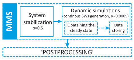
Figure 2: Algorithm of the SW dynamics calculations by MMS. MMS consist of two steps. in the first step the system is stabilizing–the equilibrium magnetic configuration is obtained. In the second step using the stabilized magnetic configuration SWs are generated by applying small rf magnetic field. The data stored during MMS are processed during the stage called ‘POSTPROCESSING’–the final results of the SW dynamics are extracted.

To generate Gaussian beam of SWs we introduce a narrow rectangular area (excitation area, marked in Fig. 1 with orange dashed lines) with a long side parallel to the expected wave fronts (along $x^{\prime}$ axis). Within the excitation area we introduce a radio-frequency (rf) magnetic field oscillating at frequency of $35$ GHz, $h_{\mathrm{dyn}}\left(x^{\prime},y^{\prime},t\right)=h_{0}(x{{}^{\prime}},y^{\prime})\exp\left(\mathrm{i}\omega t\right))$. The field $h_{\mathrm{dyn}}$ is perpendicular to the static magnetic field and its amplitude changes along the $x^{\prime}$-axis according with the Gauss distribution $G(x)=\exp\left[2\left(x{{}^{\prime}}-x_{0}{{}^{\prime}}\right)^{2}/\left(l\sigma\right)^{2}\right]$ and along $y^{\prime}$-axis takes uniform, non-zero values only for small window of width $w=5$ nm centered around $y_{0}{{}^{\prime}}$ . $l$ is the length of the excitation area (in our simulations $l=1.5$ μm) and $\sigma^{2}$ ($\sigma=0.2$) is a parameter which can be treated as variance of the Gauss distribution centered around $x_{0}{{}^{\prime}}$. Hence, $h_{0}\left(x^{\prime},y^{\prime}\right)=h\Theta_{\mathrm{H}}(y{{}^{\prime}}-y_{0}{{}^{\prime}}+w/2)\Theta_{\mathrm{H}}(-y{{}^{\prime}}+y_{0}^{{}^{\prime}}+w/2)G(x{{}^{\prime}})$, where $\Theta_{\mathrm{H}}$ is the Heaviside step function. We assume that $h=0.02H$ being maximum amplitude of the rf magnetic field which needs to be small to stay in linear regime. Example result of MMS is shown in Fig. 3.

Extracting the precise value of the shift of SW beam $\Delta X$ from MMS results requires the following three-stage procedure. In the first stage we extract a series of SW intensity profiles using an array of screen detectors parallel to the $y$-axis for different locations ($x_{j}$) along the film edge but far enough from the reflection point, i.e., out of the interference pattern of SW near the reflection point. At every point $x_{j}$ the intensity was calculated using equation: $I_{x_{j}}\left(y\right)=\int_{0}^{4T}\left|m_{z}\left(x_{j},y,t\right)\right|\mathrm{d}t$, where $T=1/f$ and $m_{z}$ is the component of the magnetization vector perpendicular to the film plane. In the next stage, using Gaussian fitting, we have extracted positions of centers of the intensity profiles for every $y_{j}(x_{j})$. Having series of the peak positions and its locations along $y$ (red and blue full dots in Fig. 3 for the incident and reflected beams, respectively) we can extract rays of the incident and reflected SW beams (red and blue solid line in Fig. 3, respectively). Finally, the value of the shift $\Delta X$ can be easily calculated with small errors up to several nanometers.

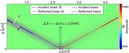
Figure 3: Exemplary result of MMS showing the color map of the dynamic magnetization amplitude of the SW beam at reflection from the edge of the YIG film. The presented result was achieved for $K_{\mathrm{S}}=-0.1$ mJ/m². At this value of the surface anisotropy the negative value of SW beam shift is observed: $\Delta X=-45.8$ nm. The blue line corresponds to the rays of the incident beam and red line to the reflected beam. The dashed white line close to the ray of the incident beam points at the direction of the SW wavevector.

II Results and discussion

Result of the pure GH shift in dependence on the pinning parameter obtained from the analytical model [Eq. (14)] is presented in Fig. 4(a). This dependence $\Delta X_{\mathrm{GH}}(d)$ is an antisymmetrical function with respect to $d=0$ and has maximum and minimum value for $d<0$ and $d>0$, respectively. The effective pinning parameter $d$ has contributions from the exchange interaction, dipole interaction and magnetic surface anisotropy. To study influence of the magnetic anisotropy we show also $\Delta X$ in dependence on $K_{\mathrm{s}}$ in Fig. 4(b) with solid line. GH shift exists for $K_{\mathrm{s}}=0$ (marked with small square in Fig. 4(b)) due to effective pinning coming from the dipole interactions(Guslienko05, ) and is $\text{\leavevmode{D}}X_{\mathrm{GH}}=-17.0$ nm. $\Delta X_{\mathrm{GH}}$ takes maximum absolute values for $K_{\mathrm{s}}=0.271$ mJ/m² and $K_{\mathrm{s}}=-0.153$ mJ/m². $\Delta X_{\mathrm{GH}}=0$ for $K_{\mathrm{s}}=0.59$ mJ/m², this is when magnetic surface anisotropy compensate the effect of the dipole interactions at the film edge. For large negative and positive values of $K_{\mathrm{S}}$ the GH shift tends monotonously to zero. This shows that the measure of the GH shift can be used to indicate the surface magnetic anisotropy at the thin film edge locally, especially in the range of its sudden change, i.e., between $-0.153$ and $0.271$ mJ/m². To test this possibility we perform MMS according with the procedure described in section I.3.

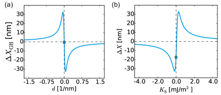
Figure 4: Analytical results of the GH shift in the reflection of the SW beam from edge of the thin YIG film calculated using Eq. (14) in dependence on (a) pinning parameter $d$ and (b) magnetic surface anisotropy constant $K_{\mathrm{s}}$. The blue squares corresponds to values of GH shift for $d=0$ in (a) and $K_{\mathrm{s}}=0$ in (b).

Dependence of the SW beam shift on the surface anisotropy constant obtained from MMS for $\mu_{0}H=0.7$ T in thin YIG film is presented in Fig. 5 with green solid dots. The value of the shift for $K_{\mathrm{s}}=0$ obtained from MMS is $\Delta X=-32.4$ nm and this is significantly larger than the GH shift obtained from analytical solutions ($\Delta X_{\mathrm{GH}}=-9$ nm). The maximal value of $\Delta X=13.83$ nm is found for $K_{\mathrm{s}}=0.25$ mJ/m² and minimal is $\Delta X=-49.6$ nm for $K_{\mathrm{s}}=-0.2$ mJ/m², i.e., out of the scale presented in Fig. 5. This dependence is quantitatively similar to the function obtained in the analytical model (Fig. 4). Nevertheless, there are distinct differences between both results.

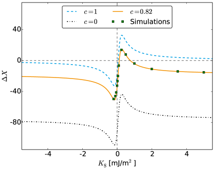
Figure 5: Results of the MMS (green solid points) and obtained from the analytical models presenting dependence of the SW beam shift on the surface magnetic anisotropy constant in the YIG film in the external field $0.7$ T. Only the results for fully saturated sample $K_{\mathrm{s}}\geq K_{0}$ ($K_{0}=-0.22$ mJ/m²) are shown. Dashed blue line corresponds to basic analytical model for GH shift [Eq. (14)] without included SWs bending corrections ($c=1$). Dash-dotted black line presents results for the analytical model [Eq. (20)] with $c=0$. Solid orange line correspond to results of the analytical model with fitted $c=0.82$.

The analytical model is based on number of assumptions which are absent in MMS, thus there is a disagreement between both results. The full saturation of the magnetization is important assumption made in the analytical model. Surface magnetic anisotropy at the edge of the film increases (or decreases) a value of a total internal magnetic field at this edge. This change of the internal magnetic field in the single computational cell at the edge is equal to the surface anisotropy field $\mu_{0}H_{\mathrm{s}}=2K_{\mathrm{s}}/\left(M_{\mathrm{s}}l_{y}\right)$. Therefore, exactly at the film edge the demagnetizing field can be compensated or enhanced by surface anisotropy field, in dependence on the sign of $K_{\mathrm{s}}$. When surface anisotropy constant $K_{\mathrm{s}}=K_{0}=-\frac{1}{2}\mu_{0}L_{z}M_{\mathrm{s}}\left(H-M_{\mathrm{s}}\right)\thickapprox-0.22$ mJ/m² the total internal field at the surface is equal $0$ (the demagnetizing field at the edge is compensated by the anisotropy field). Hence, for $K_{\mathrm{s}}<K_{0}$ the equilibrium orientation of the magnetization at the edge of the film rotates from the saturation direction (this is transformation from the easy axis to the easy plane configuration). This is demonstrated in Fig. 6 (b), where magnetization components along $x$, $y$ and $z$ axis are presented as a function of the distance from the film edge for $K_{\mathrm{s}}=-2.0$ mJ/m². We can see the rotation of the magnetization from the $y$ direction (saturation direction) towards the $x$ axis. The change of the magnetization configuration is not taken into account in the model developed in Sec. I.2. Moreover, in real sample there is a possibility for appearing domain walls along the film edge, which can create additional factor for complexity of the problem. Therefore, in this paper we limit the analysis to the fully saturated sample, i.e., when $K_{\mathrm{s}}\geq K_{0}$ (we note, that the exact value of $K_{0}$ depends on the magnitude of the external magnetic field).

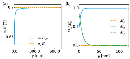
Figure 6: (a) Effective magnetic field along the $y$-axis inside YIG film for $K_{\mathrm{s}}=0$ is shown with blue solid line, orange dashed line corresponds to the external magnetic field (0.7 T). (b) Static magnetic configuration in the vicinity of thin YIG film edge for $K_{\mathrm{s}}=-2$ mJ/m² (i.e., $K_{\mathrm{s}}<K_{0}$); blue solid, orange dashed and green dash-dotted line marks $x$, $y$ and $z$ component of the magnetization vector normalized to unity, respectively.

The model shown in Sec. I.2 doesn’t take into account influence of inhomogeneity of the internal magnetic field on the behavior of propagating beam especially in the vicinity of the film edge. It is probably the next most important factor, which makes a comparison of the analytical and MMS results difficult for the saturate state. In MMS, and in a real sample, the magnetization which is perpendicular to the film edge creates an inhomogeneous static demagnetizing field, which is directed opposite to the magnetization saturation. In result, the internal magnetic field decreases monotonically when moving from the film center towards its edge [solid-blue line in Fig. 6(a)]. In our interpretation this inhomogeneity is responsible for a shift of $\Delta X$ in MMS towards negative values as compared to the results of Eq. (14) [see, Fig. 6]: for very high positive $K_{\mathrm{s}}$ the $\Delta X_{\mathrm{GH}}$ monotonously tends to $0$ in the analytical model [Fig. 4(b)], while results of the MMS show that the value of $\Delta X$ reaches non-zero negative value even for very high value of $K_{\mathrm{s}}$ ($\Delta X=-15.2$ nm for $K_{\mathrm{s}}=10$ mJ/m²). This means, that the inhomogeneity of the internal magnetic field in the close vicinity of the thin film edge causes an increase of the refractive index for SWs (Kim08, ; Vansteenkiste14, ) and consequently results in bending of the SW beam and changes the shift measured in far field.

Here, we propose the simple analytical model of the wave bending, which allows to estimate factor which correct the value of the GH SW beam’s shift obtained from Eq. (14). We will consider gradual change of the refractive index for SWs in the vicinity of the film edge.

Similarly as in optics, the refraction law for SWs (i.e., Snell law) can be concluded from analysis of the isofrequency contours and momentum conservation of the wavevector component parallel to the edge ($k_{x}=\mathrm{const.}$). Let us assume, that full distance of the gradual change of the refractive index in thin film can be divided into $N$ thin slices, numbered with integer $n$. Therefore, we can assume multiple refractions on $(N-1)$ parallel planes, separating neighbor slices [Fig. 7(b)]. At the plane between two arbitrary slices $n$ and $n+1$ according to Snell low $\left(k_{n}\sin\theta_{\text{i},n}=k_{n+1}\sin\theta_{\text{i},n+1}\right)$ [Fig. 7(a)]. Thus, we can calculate final angle of incidence after passing $N$ slices: $\sin\theta_{\mathrm{i},N}=\frac{k_{0}}{k_{N}}\sin\theta_{\mathrm{i},0}$, where $k_{N}$ and $\theta_{\mathrm{i},N}$ are wavenumber and incident angle in the last slice. $k_{0}\equiv k(y_{0})$ and $\theta_{\mathrm{i},0}$ are wavenumber and incident angle in the initial media, i.e., in the interior far from the edge of the film. Rewriting the expression for space coordinates (substitute $k(y)\equiv k_{N}$ and $\theta_{\mathrm{i}}(y)\equiv\theta_{\mathrm{i},N}$) we obtain:

$$\theta_{\mathrm{i}}(y)=\arcsin\left(\frac{k_{0}}{k(y)}\sin\theta_{\mathrm{i},0}\right).$$ (15)

From here, the final value of $\theta_{\mathrm{i}}(y)$ at the $y$ distance from the film edge can be calculated, if the value of $k(y)$, initial values of the wavevector $k_{0}$ and the initial angle of the incidence $\theta_{\mathrm{i},0}$ are known.

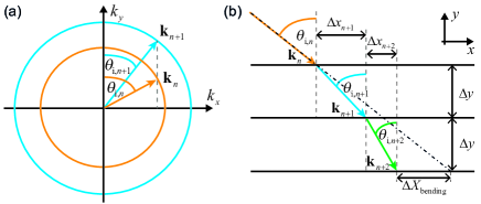
Figure 7: (a) Explanation of the refraction of the wave on the interface between media with low refractive index ($n$-th slice, orange line) and high refractive index ($n+1$ slice, blue line) based on isofrequency contours analysis. The conservation of the $x$ components of the wavevectors in the refraction is required by the translational symmetry along the $x$. (b) Example of two refractions on the interfaces between $n$-th and $n+1$, and between $n+1$ and $n+2$ slice. The refractive index increases with increasing index $n$. The beam shift $\Delta X_{\mathrm{bending}}$ resulting from the bending is shown schematically.

The knowledge of the incident angle at the vicinity of the film edge $\theta_{\mathrm{i}}(y)$ allows us to derive formula which describes propagation of the beam through the area of gradually changed refractive index. Similarly to previous approach, let us consider single refraction on the interface between $n$ and $n+1$ slice, as it is shown in Fig. 7(b). Projection of the beam path onto the direction tangential to the interface is $\Delta x_{n+1}=\Delta y\tan\theta_{\mathrm{i},n+1}$ where $\Delta y$ is the thickness of the slice (we assume here for simplicity slices of the same thickness). Generalizing this formula for cascading refraction on $N$ slices we obtain:

$$x_{N} = \sum_{n=1}^{N}\Delta x_{n}=\Delta y\sum_{n=1}^{N}\tan\theta_{\mathrm{i},n}$$ (16)

$$= \Delta y\sum_{n=1}^{N}\tan\arcsin\left(\frac{k_{0}}{k_{n}}\sin\theta_{\text{i},0}\right)$$

Assuming infinitesimally small distance between interfaces $\Delta y\rightarrow dy$ we can transform summation into integration along the $y$ axis between initial point of the SW generation $y_{0}$ and the point of the reflection $y_{N}$:

$$x(y_{0},y_{N}) = \int_{y_{0}}^{y_{N}}\mathrm{d}y\tan\arcsin\left(\frac{k_{0}}{k_{n}}\sin\theta_{\text{i},0}\right)$$ (17)

$$= \int_{y_{0}}^{y_{N}}\mathrm{d}y\frac{\sin\theta_{\text{i},0}}{\sqrt{\left(\frac{k(y)}{k_{0}}\right)^{2}-\sin^{2}\theta_{\text{i},0}}}.$$

Therefore, if the edge where reflection takes place is located at $y_{N}=0$ (like in Fig. 1), the SW beam shift introduced by bending and measured in far field (observation point is assumed at the same distance from the edge as the source of the SW) is described by following formula:

$$\Delta X_{\mathrm{bending}}=2\left[y_{0}\tan\theta_{\mathrm{i}}-x(y_{0},0)\right],$$ (18)

where factor 2 is included to take into account the beam way from source to the edge and after reflection to the observation point.

The total shift of the SW beam observed in far field is a sum of the GH shift and the shift resulting from the bending:

$$\Delta X=\Delta X_{\mathrm{bending}}+\Delta X_{\mathrm{GH}}.$$ (19)

Eq. (19) is a general formula describing a total shift of the wave beam propagating in media with gradual change of the refractive index. Way of the beam ray depends on relation describing $\mathbf{k}(y)$. And this is main bottleneck in this approach: unknown formula for wavevector of the SW in dependence on $y$ in an area of the inhomogeneous effective magnetic field. However, knowledge of the dispersion relation in homogeneous film, Eq. (5), can help in qualitative modeling of the total shift of the SW beam also in a part of the film with gradual change of the refractive index.

Demagnetization field decreases a value of the internal magnetic field, its dependence on distance from the edge can be expressed by the relation: $H_{\mathrm{d}}(y)=4M_{\mathrm{S}}\arctan\left[L_{z}/(2y)\right]$.(Joseph65, ) This field far from the edge of the film tends to zero [Fig. 5 (a)]. We can substitute bias magnetic field in Eq. (5) with the internal field $H\rightarrow H(y)\equiv H-H_{\mathrm{d}}(y)$. This approach should be valid for slow change of $H_{\mathrm{d}}(y)$ with distance. However, in the vicinity of the thin film edge we observe a rapid change of the demagnetizing field [Fig. 6(a)] and the plane-wave approximation fails. Therefore, we propose to introduce homotopic transformation of the demagnetizing field: $H(y)=H-\left[cH_{\mathrm{d}}(y_{0})+\left(1-c\right)H_{\mathrm{d}}(y)\right]$ with parameter $c\in\left[0,1\right]$, which will reduce influence of the rapid changes of the demagnetizing field on wave vector. Then, the wave vector magnitude can be described by the following equation:

$$k^{2}(y,\theta_{\mathrm{i}}) = \frac{\mu_{0}M_{\mathrm{S}}}{4A}\Biggl{(}-2\left(H-\left[cH_{\mathrm{d}}(y_{0})+\left(1-c\right)H_{\mathrm{d}}(y)\right]\right)$$ (20)

$$-M_{\mathrm{S}}\sin^{2}\theta_{\mathrm{i}}+\sqrt{\frac{4\omega^{2}}{\mu_{0}^{2}\gamma^{2}}+M_{\mathrm{S}}^{2}\sin^{4}\theta_{\mathrm{i}}}\Biggr{)},$$

where $y_{0}$ can be interpreted as position of the source of the SW beam, i.e., the position where the demagnetizing field magnitude is close to zero.

Now, the only issue is a correct choice of the parameter $c$ in Eq. (20) to find $k(y)$, and to fit $\Delta X(K_{\mathrm{s}})$ dependence to the curve obtained from MMS. Taking $c=1$ we assume, that isofrequency contours are the same in whole sample ($k$ does not depend on $y$), the wave propagate in homogeneous internal magnetic field equal $H$ [because $H_{d}(y_{0})\cong 0$] and Eq. (20) reduces to Eq. (5). In this case $\Delta X_{\mathrm{bending}}=0$ and $\Delta X=\Delta X_{\mathrm{GH}}$, i.e, the total shift is equal to Eq. (14). The obtained curve is plotted in Fig. 5 with blue dashed line. In opposite limit, $c=0$ the dependence $k(y)$ follows exactly the change of $H_{\mathrm{d}}(y)$. In this case the $\Delta X_{\mathrm{total}}(K_{\mathrm{s}})$ calculated from Eq. (19) is shown in Fig. 5 with black dotted line. It takes value $\Delta X=\Delta X_{\mathrm{bending}}=-79$ nm for large $K_{\mathrm{s}}$, much below the value obtained from MMS. This discrepancy exists, because for each $y$ we took in calculation of the $\Delta X_{\mathrm{bending}}$ [in the integral Eq. (17)] the dispersion relation Eq. (20) which is for the film with homogenous magnetic field. In real situation, the dispersion relation in the area of inhomogeneous refractive index will be different from the local value. Thus averaging of the demagnetizing field across some distance shall improve the estimation. Moreover, the $c$ shall depend on the relative value of the wavelength to the special changes of the refractive index. Thus, the value of $c$ from Eq. (20) needs to be treated as a parameter, which includes an effective influence of the inhomogeneity of the refractive index on the dispersion relation of SWs. For $c=0.82$ we have obtained very good agreement between results of MMS and analytical model $\Delta X(K_{\mathrm{s}})\approx\Delta X(K_{s})$ for $K_{\mathrm{s}}>-0.22$ mJ/m², as it is shown in Fig. 6 with orange solid line.

The value of ΔX is very sensitive for small change of $K_{\mathrm{s}}$ between the extremes. The magnetic surface anisotropy in ferromagnetic films can take different values, however the most interesting is the range around $0$, where the transition from easy axis into easy-plane anisotropy takes place. Thus, the measure of the SW beam’s shift can indicate the local surface magnetic anisotropy at the film edge with spatial resolution limited by the size of the width of the SW beam. This information shall be important also for understanding and exploiting SW excitations and actuation at the surface of YIG film being in contact with Pt, where the magnetic surface anisotropy was shown to play a significant role in the spin pumping.(Xiao12, ; daSilva13, ; Reshetnyak04, ; Zhou13, ) Further investigation is required to test an influence of the second ferromagnetic material attached to the YIG film edge on the SW reflection. Here, extension of the analytical model with properly defined boundary conditions will be required.(Skarsvag14, ; Kruglyak14, )

The micromagnetic simulations were conducted for the value of the damping parameter $\alpha=0.0005$, which is close to the value of thickSerga12 and also very thin films (tens of nm thick) of YIG as demonstrated experimentally recently.Jungfleisch15 We have performed additional simulations for slightly smaller and larger damping to check the influence of damping on GH shift. Apart from increase of the amplitude of the reflected SW beam with decreasing $\alpha$ the results of the GH shift are very close to those presented in the manuscript. This indicates that small changes of the homogeneous damping does not affect GH shift. However, for the electromagnetic waves reflected from the interface GH shift is strongly affected if the reflected material is a medium with strong absorption,(Wild82, ; Chern14, ) where the absorption can even change the sign of the GH shift. Thus, we can suppose, that also in magnonics the inhomogeneous damping, especially with its high value at the interface or in the media behind the reflection edge, will influence GH shift. Further investigations are necessary to elucidate the role of inhomogeneous damping on the GH shift in the reflection of SWs from the edge or interface ferromagnetic films.

III Conclusions

We have performed analytical and numerical study of the SWs beams shift at the reflection from the edge of the YIG thin film in dependence on the surface magnetic anisotropy present at the film edge. The GH effect and SW bending are shown to contribute to the SW beam’s shift measured in far field. We have shown that the GH shift is modulated in a broad range by changes of the surface magnetic anisotropy constant between two extremes: $K_{\mathrm{s,min}}=-0.155$ mJ/m² and $K_{\mathrm{s,max}}=0.275$ mJ/m². It means that even small change of the surface magnetic anisotropy, some imperfections or changes in a surrounding of the film edge can result in significant change in the reflected SW beams position in far field. The demagnetizing field gradually changes the refractive index of SWs of the film with its sudden increase near the film’s edge. This variation of the refractive index bends the SW propagating towards (and outwards) of the edge and introduce additional shift of the SW beam. However, this shift is independent on the surface magnetic anisotropy. For large positive values of $K_{\mathrm{s}}$ the value of $\Delta X$ is almost insensitive to changes of the magnitude of the magnetic surface anisotropy and is mainly a result of the SW bending due to gradually increased refractive index at the film edge. These results shall be of importance for magnonics, its applications for sensing and also for developing a new direction of research devoted to metamaterial properties for SWs, especially the graded index magnonics.

Appendix A Green functions

The $x$ and $z$ components of the magnetostatic fields can be expressed as:

$$h_{x}(x,y)=\int dx^{\prime}dy^{\prime}G_{xx}(x,y;x^{\prime},y^{\prime})m_{x}(x^{\prime},y^{\prime}),$$

$$h_{z}(x,y)=\int dx^{\prime}dy^{\prime}G_{zz}(x,y;x^{\prime},y^{\prime})m_{z}(x^{\prime},y^{\prime}),$$ (21)

where

$$G_{\alpha\beta}(\mathbf{\rho};\mathbf{\rho}^{\prime}) = \frac{1}{(2\pi)^{2}}\int d^{2}\mathbf{k}G_{\alpha\beta}(\mathbf{k})\text{e}^{i\mathbf{k}\cdot(\mathbf{\rho}-\mathbf{\rho}^{\prime})},$$ (22)

$$G_{xx}(\mathbf{k}) = -f(kL_{z})\frac{k_{x}^{2}}{k^{2}},\;\;G_{zz}(\mathbf{k})=-\left[1-f(kL_{z})\right],$$

and function $f$ is defined in Eq. (3).

Substituting $m_{\alpha}(x,y)=\exp{(ik_{x}x)}m_{\alpha}(y)$ to Eq. (21) and performing integration over $x^{\prime}$ and $k_{x}$we can get the dipolar field in the form

$$h_{\alpha}(x,y)=\text{e}^{ik_{x}x}\int dy^{\prime}g_{\alpha\alpha}(y,y^{\prime})m_{\alpha}(y^{\prime}),$$ (23)

where the magnetostatic kernels are calculated using Ref. [Gradshteyn, ]:

$$g_{zz}(\eta)=\frac{1}{\pi L_{z}}\left[K_{0}\left(k_{x}\sqrt{L_{z}^{2}+\eta^{a}}\right)-K_{0}(k_{x}|\eta|)\right]$$ (24)

and

$$g_{xx}(\eta)=-\frac{1}{2}k_{x}\text{e}^{-k_{x}|\eta|},\;\;\text{at}\;\;k_{x}L_{z}\gg 1,$$ (25)

above, $K_{0}$ is the modified Bessel’s function of the zero order, and $\eta=y-y^{\prime}$. The $zz$-component of the magnetostatic kernel in Eq. (24) has logarithmic singularity at $\eta=0$. The component $g_{xx}(\eta)$ has sharp maximum at $\eta=0$ because of the condition $k_{x}L_{z}\gg 1$. This justify using the Taylor series decomposition near the point $\eta=0$ calculating the dynamical dipolar fields and derivation of the boundary conditions given by Eqs. (10) and (11).

Appendix B Reflection coefficient

The plane wave solutions are assumed for the dynamic components of the magnetization vector $m_{\alpha}(\mathbf{r},t)$:

$$m_{\alpha}(\mathbf{r},t)=A_{\alpha}\text{e}^{i\left(\mathbf{k}_{\mathrm{i}}\cdot\mathbf{r}-\omega t\right)}+B_{\alpha}\mathrm{e}^{i\left(\mathbf{k}_{\mathrm{r}}\cdot\mathbf{r}-\omega t\right)},$$ (26)

by substituting this solution to the boundary condition (6) we obtain:

$$\left[ik_{\mathrm{i},y}A_{\alpha}\mathrm{e}^{i\left(\mathbf{k}_{\mathrm{i}}\cdot\mathbf{r}-\omega t\right)}-ik_{\mathrm{r},y}B_{\alpha}\mathrm{e}^{i\left(\mathbf{-k}_{\mathrm{r}}\cdot\mathbf{r}-\omega t\right)}\right.$$ (27)

$$+ \left.d\left(A_{\alpha}\mathrm{e}^{i\left(\mathbf{k}_{\mathrm{i}}\cdot\mathbf{r}-\omega t\right)}+B_{\alpha}\mathrm{e}^{i\left(\mathbf{-k}_{\mathrm{r}}\cdot\mathbf{r}-\omega t\right)}\right)\right]_{y=0}=0.$$

At the reflection point $k_{\mathrm{i},x}=k_{\mathrm{r},x}\equiv k_{x}$ and $k_{\mathrm{i},y}=-k_{\mathrm{r},y}\equiv k_{y}$ we get:

$$ik_{y}A_{\alpha}-ik_{y}B_{\alpha}+d(A_{\alpha}+B_{\alpha})=0.$$ (28)

Finally, the formula (12) for refractive index can be easily derived:

$$R\equiv\frac{B_{\alpha}}{A_{\alpha}}=\frac{ik_{y}+d}{ik_{y}-d}=\frac{i\sqrt{k^{2}-k_{x}^{2}}+d}{i\sqrt{k^{2}-k_{x}^{2}}-d}.$$ (29)

- (1) J. Shibata Y. Otani, Phys. Rev. B 70, 012404 (2004).
- (2) Y. Kajiwara, K. Uchida, D. Kikuchi, T. An, Y. Fujikawa and E. Saitoh, Appl. Phys. Lett. 103, 052404 (2013).
- (3) R. L. Stamps et al., J. Phys. D: Appl. Phys. 47, 333001 (2014).
- (4) M. Krawczyk,D. Grundler , J. Phys.: Condens. Matter 26, 123202 (2014 ).
- (5) A. V. Chumak, A. A. Serga and B. Hillebrands, Nat. Commun. 5, 4700 (2014).
- (6) V. V. Kruglyak, S. O. Demokritov and D. Grundler, J. Phys. D: Appl. Phys. 43, 264001 (2010).
- (7) S. O. Demokritov and A. N. Slavin (eds.) Magnonics from fundamentals to applications (Berlin: Springer, 2013).
- (8) A. Khitun, J. Appl. Phys. 111, 054307 (2012).
- (9) M. P. Kostylev, A. A. Serga, T. Schneider, T. Neumann, B. Leven, B. Hillebrands and R. L. Stamps, Phys. Rev. B 76, 184419 (2007).
- (10) A. V. Chumak, A. A. Serga, S. Wolff, B. Hillebrands and M. P. Kostylev, Appl. Phys. Lett. 94, 172511 (2009).
- (11) M. Dvornik, A. N. Kuhko and V. V. Kruglyak, J. Appl. Phys. 109, 07D350 (2011).
- (12) S.-K. Kim, S. Choi, K.-S. Lee, D.-S. Han, D.-E. Jung and Y.-S. Choi, Appl. Phys. Lett. 92, 212501 (2008).
- (13) G. A. Vugal’ter and A. G. Korovin, Radiofizika 31, 1126 (1988).
- (14) R. E. Floyd and J. C. Sethares, J. Appl. Phys. 55, 2515 (1984).
- (15) T. Schneider, A. V. Chumak, C. W. Sandweg, S. Trudel, S. Wolff, M. P. Kostylev, V. S. Tiberkevich, A. N. Slavin and B. Hillebrands, Phys. Rev. Lett. 104 197203 (2010).
- (16) R. Gieniusz, H. Ulrichs, V. D. Bessonov, U. Guzowska, A. I. Stognii and A. Maziewski, Appl. Phys. Lett. 102, 102409 (2013).
- (17) M. P. Kostylev, A. A. Serga and B. Hillebrands, Phys. Rev. Lett. 106, 134101 (2011).
- (18) J. W. Boyle, S. A. Nikitov, A. D. Boardman, J. G. Booth and K. Booth, Phys. Rev. B 53, 12173 (1996).
- (19) M. Bauer, C. Mathieu, S. O. Demokritov, B. Hillebrands, P. A. Kolodin, S. Sure, H. Dötsch, V. Grimalsky, Yu. Rapoport and A. N. Slavin, Phys. Rev. B 56, R8483 (1997).
- (20) F. Goos and H. Hänchen, Ann. Phys. (Leipzig) 436 333 (1947).
- (21) N. F. Declercq and E. Lamkanfi, Appl. Phys. Lett. 93 054103 (2008).
- (22) M. Sharma and S. Ghosh, J. Phys.: Condens. Matter 23 055501 (2011).
- (23) V. -O. de Haan, J. Plomp, T. M. Rekveldt, W. H. Kraan, A. A. van Well, R. M. Dalgliesh and S. Langridge, Phys. Rev. Lett. 104, 010401 (2010).
- (24) Yu. S. Dadoenkova et al., Appl. Phys. Lett. 101, 042404 (2012).
- (25) P. Gruszecki et al. Appl. Phys. Lett. 105 242406 (2014).
- (26) A. A. Serga, A. V. Chumak and B. Hillebrands, J. Phys D: Appl. Phys. 43, 264002 (2012).
- (27) Y. Sun, Y.-Y. Song, H. Chang, M. Kabatek, M. Jantz, W. Schneider, M. Wu, H. Schultheiss and A. Hoffmann, Appl. Phys. Lett. 101, 152405 (2012).
- (28) Y. Sun et al., Phys. Rev. Lett. 111, 106601 (2013).
- (29) T. Liu, H. Chang, V. Vlaminck, Y. Sun, M. Kabatek, A. Hoffmann, L. Deng and M. Wu, J. Appl. Phys. 115 17A501 (2014).
- (30) P. Pirro, T. Brächer, A. V. Chumak, B. Lägel, C. Dubs, O. Surzhenko, P. Görnert, B. Leven and B. Hillebrands, Appl. Phys. Lett. 104, 012402 (2014).
- (31) J. M. Shaw, S. E. Russek, T. Thomson, M. J. Donahue, B. D. Terris, O. Hellwig, E. Dobisz and M. L. Schneider, Phys. Rev. B 78 024414 (2008).
- (32) S. Putter, N. Mikuszeit, E. Y. Vedmedenko and H. P. Oepen, J. Appl. Phys. 106, 043916 (2009).
- (33) O. Ozatay et al., Natture Materials 7, 567 (2008).
- (34) J. Xiao and G. E. W. Bauer, Phys. Rev. Lett. 108, 217204 (2012).
- (35) G. L. da Silva, L. H. Vilela-Leao, S. M. Rezende and A. Azevedo, Appl. Phys. Lett. 102, 012401 (2013).
- (36) P. Yen, T. S. Stakelon and P. E. Wigen, Phys. Rev. B 19, 4575 (1979).
- (37) P. Bruno and J. P. Renard, Appl. Phys. A 49, 499 (1989).
- (38) U. Gradmann, J. Magn. Magn. Matter. 54-57, 733 (1986).
- (39) M. T. Johnson, P. J. H. Bloemen, F. J. A. den Broeder and J. J. de Vries, Rep. Prog. Phys. 59 1409 (1996).
- (40) M. Jamet, W. Wernsdorfer, C. Thirion, V. Dupuis, P. Mélinon, A. Pérez and D. Mailly, Phys. Rev. B 69, 024401 (2004).
- (41) B. A. Kalinikos and A. N. Slavin, J. Phys. C: Solid State Phys. 19, 7013 (1986).
- (42) G.T. Rado and J. R. Weertman, J. Phys. Chem. Solids 11, 315 (1959).
- (43) K. Y. Guslienko and A. N. Slavin, Phys. Rev. B 72, 014463 (2005).
- (44) K. Y. Guslienko, S. O. Demokritov, B. Hillebrands, and A. N. Slavin, Phys. Rev. B 66, 132402 (2002).
- (45) K. Y. Guslienko, and A. N. Slavin, J. Magn. Magn. Mat. 323, 2418 (2011).
- (46) K. Artmann Ann. Phys. (Leipzig) 2, 87 (1948).
- (47) G. Venkat, D. Kumar, M. Franchin, O. Dmytriiev, M. Mruczkiewicz, H. Fangohr, A. Barman, M. Krawczyk and A. Prabhakar, IEEE Trans. Magn. 49, 524 (2013).
- (48) W. Kim, S.-W. Lee and K.-J. Lee, J. Phys. D: Appl. Phys. 44 384001 (2011).
- (49) R. Hertel, W. Wulfhekel and J. Kirschner, Phys. Rev. Lett. 93, 257202 (2004).
- (50) K. M. Lebecki, M. J. Donahue and M. W. Gutowski, J. Phys. D, Appl. Phys. 41, 175005 (2008).
- (51) A. Vansteenkiste, J. Leliaert, M. Dvornik, M. Helsen, F. Garcia-Sanchez and B. Van Waeyenberge, AIP Advances 4, 107133 (2014).
- (52) It is important to note an influence of used in MMS finite difference (FD) cells dimensions on the obtained results, especially when a surface magnetic anisotropy is included. Due to specification of FD method used in MuMax3, where only volume anisotropy is included, surface anisotropy have to be introduced in indirect way. We’ve assumed volume anisotropy in one row of finite difference cells along edge of the film (at ). In this case , where is Dirac delta function. MMS confirmed that the size of cell influences the results of simulations in the scale below the exchange length. However, we have verified numerically, that in the performed here MMS there is only slight change of the obtained values with further decrease of the unit cell, i.e., for nm the convergence is achieved.
- (53) R. I. Joseph and E. Schloemann, J. Appl. Phys. 36, 1579 (1965);
- (54) S. A. Reshetnyak, Physics of the Solid State 46, 1061 (2004).
- (55) Y. Zhou, H. Jiao, Y. -T. Chen, G. E. W. Bauer and J. Xiao, Phys. Rev. B 88, 184403 (2013).
- (56) H. Skarsvag, A. Kapelrud and A. Brataas, Phys. Rev. B 90, 094418 (2014).
- (57) K. Y. Guslienko, R. W. Chantrell, and A. N. Slavin, Phys. Rev. B 68, 024422 (2003).
- (58) V. V. Kruglyak, O. Yu. Gorobets, Yu. I. Gorobets and A. N. Kuchko, J. Phys.: Condens. Matter 26, 406001 (2014)
- (59) M. B. Jungfleisch, et al., J. Appl. Phys. 117, 17D128 (2015).
- (60) W. J. Wild and C. Lee Giles, Phys. Rev. a 25, 2099 (1982).
- (61) R.-L. Chern, J. Opt. Soc. Am. B 31, 1174 (2014).
- (62) I. S. Gradshteyn and I. M. Ryzhik, Tables of Integrals, Series and Products, 7th ed. (Academic Press, New York, 2007).