Stochastic determination of matrix determinants

Abstract

Matrix determinants play an important role in data analysis, in particular when Gaussian processes are involved. Due to currently exploding data volumes, linear operations – matrices – acting on the data are often not accessible directly but are only represented indirectly in form of a computer routine. Such a routine implements the transformation a data vector undergoes under matrix multiplication. While efficient probing routines to estimate a matrix’s diagonal or trace, based solely on such computationally affordable matrix-vector multiplications, are well known and frequently used in signal inference, there is no stochastic estimate for its determinant. We introduce a probing method for the logarithm of a determinant of a linear operator. Our method rests upon a reformulation of the log-determinant by an integral representation and the transformation of the involved terms into stochastic expressions. This stochastic determinant determination enables large-size applications in Bayesian inference, in particular evidence calculations, model comparison, and posterior determination.

Keywords: Determinants – Stochastic Estimation – Operator Probing – Big Data – Signal Inference

I Motivation

Current and future physical observations generate huge data streams to be analyzed. Particle physics, biophysics, astronomy, and cosmology are representatives of current scientific fields of interest that are undergoing a revolution driven by increasing data volume. Typical large data sets in cosmology are, for instance, observations of the cosmic microwave background Bennett et al. (2013); Planck Collaboration et al. (2014a) as well as of the large-scale structure York et al. (2000); Spergel et al. (2007); Hill et al. (2008) as they are often wide- or all-sky observations carried out by telescopes with remarkable resolution. In order to extract information about the universe or physics in general, Bayesian inference methods becomes more and more frequently used as their large computational demands become more feasible thanks to technology developments. The signal of interest to be extracted from data could be almost everything, ranging from just a single parameter (e.g., the level of local non-Gaussianity of the cosmic microwave background Komatsu et al. (2005); Dorn et al. (2013)) to a full four-dimensional reconstruction of the structure growth in the universe Kitaura and Enßlin (2008); Jasche and Wandelt (2013). Such ambitious Bayesian analyses often invoke linear transformations of the data or of estimated signal vectors.

The size of the involved data and signal spaces often bans the explicit representation of matrices acting on these spaces by their individual matrix elements. A prominent example appearing in many analyses is, for instance, the covariance matrix of a multivariate Gaussian distribution of a vector valued quantity, which describes the two-point correlation structure of the said quantity. Due to their large dimensions such matrices are often only representable by a computer routine, which implements the application of the matrix to a vector without storing or even calculating the individual matrix elements. Such routines often invoke fast Fourier transformations and other efficient operations, which in combination render nonsparse matrices into easily computable basis systems. We refer to such a matrix as an implicit matrix. For instance, calculating the model evidence often requires calculating determinants of such matrices. This work provides an efficient way to numerically calculate determinants given only by an implicit matrix representation.

The remainder of this work is organized as follows: In Sec. II we introduce the formalism of the stochastic estimation of an implicit matrix and present two numerical examples. Section III provides a perspective of possible applications in science. Results are summarized in Sec. IV.

II Probing the log-determinant of an implicit matrix

II.1 Formalism

Let $A=(a_{ij})\in\mathds{C}^{n\times n}$ be an implicitly defined, complex-valued, square matrix of order $n$. Implicitly means that the particular entries of the matrix are not accessible, for instance, if dealing with large data sets, where an explicit storage of $A$ might exceed the memory of the computer. However, the action of the matrix as a linear operator is assumed to be known and given by a computer routine implementing the mapping $x\mapsto Ax$.

Motivated by applications in science and statistics (Secs. I and III), in particular by signal reconstruction techniques and model comparison in astronomy and cosmology, where the determinant of a covariance matrix is required (Sec. III), we constrain the variety of different types of matrices by requesting that the matrix $A$ of interest is either weak diagonal dominant or Hermitian positive definite. The term weak diagonal dominant is defined by

$$|a_{ii}|\geq\sum_{i\neq j}|a_{ij}|~{}~{}~{}\forall i,$$ (1)

while Hermitian positive definite means

$$A^{\dagger}=A~{}~{}~{}\mathrm{and}~{}~{}~{}x^{\dagger}Ax>0~{}~{}~{}\forall x\in\mathds{C}^{n}{\backslash}\{0\}$$ (2)

with ${\dagger}$ denoting the adjoint.

The diagonal and the trace of an implicit matrix can be obtained by exploiting common probing routines Selig et al. (2012); Aune et al. (2014); Hutchinson (1989); Bekas et al. (2007). A stochastic estimate of the diagonal of the linear operator $A$ is given by

$$\mathrm{diag}(A)=\left\langle\xi\star A\xi\right\rangle_{\{\xi\}}\approx\frac{1}{M}\sum_{i=1}^{M}\xi_{i}\star A\xi_{i},$$ (3)

where $\star$ denotes a componentwise product, $M=|\{\xi\}|$ the sample size, and $\left\langle\cdot\right\rangle_{\{\xi\}}$ the arithmetic mean over $\xi$ with $M\rightarrow\infty$. The probing vectors $\xi\in\mathds{C}^{n}$ are random variables, whose components $x~{}(x^{\prime})$ fulfill the condition $\left\langle\xi_{x}\xi_{x^{\prime}}\right\rangle_{\{\xi\}}=\delta_{xx^{\prime}}$. Analogously to the diagonal of an operator its trace can be probed by, e.g.,

$$\mathrm{tr}(A)=\left\langle\xi^{\dagger}A\xi\right\rangle_{\{\xi\}}.$$ (4)

Recently, there have been investigations to improve these straightforward probing methods by exploiting Bayesian inference Selig et al. (2012). This has been achieved by reformulating the process of stochastic probing of an operator’s diagonal (trace) as a signal inference problem. As a result, it requires fewer probes than the purely stochastic methods and thus can decrease the computational costs. With the phrase operator probing, be it trace or diagonal probing, we subsequently refer to the entirety of probing methods in general.

The linear operator $A$ can be split into a diagonal matrix $D\in\mathds{C}^{n\times n}$ and a matrix $N\in\mathds{C}^{n\times n}$, which contains the off-diagonal part of $A$, i.e.,

$$A=D+N.$$ (5)

We are now interested in the value of its determinant or of its log-determinant, $\Delta\equiv\ln[\mathrm{det}(A)]$. In case $A$ is mainly dominated by its diagonal (i.e. $ND^{-1}\ll\mathds{1}$ spectrally), a Taylor expansion of the log-determinant might be a reasonable approximation,

$$\begin{split}\Delta=&~{}\ln[\mathrm{det}(D+N)]\\ =&~{}\ln[\mathrm{det}(D)]+\mathrm{tr}\left[ND^{-1}\right]+\mathcal{O}\left(\mathrm{tr}\left[\left(ND^{-1}\right)^{2}\right]\right),\end{split}$$ (6)

which is sometimes feasible dealing with implicit operators, e.g., see Refs. Dorn et al. (2013, 2014) for recent applications in cosmic microwave background physics. This approximation, however, breaks down when the relation $ND^{-1}\ll\mathds{1}$ (spectrally) is violated. In order to circumvent this problem we introduce the quantity

$$\Delta(t)\equiv\ln[\mathrm{det}(D+tN)]$$ (7)

with the pseudotime parameter $t\in[0,1]$. For a sufficiently small $t$ the approximation of Eq. (6) becomes valid. This property can be used together with a few mathematical manipulations (for details see Appendix A) to obtain the formula

$$\begin{split}\Delta=&\int_{0}^{1}dt~{}\mathrm{tr}\left[N\left(D+tN\right)^{-1}\right]+\Delta(0)\\ =&~{}\int_{0}^{1}dt~{}\left\langle\xi^{\dagger}N\left(D+tN\right)^{-1}\xi\right\rangle_{\{\xi\}}+\Delta(0)\end{split}$$ (8)

that represents a stochastic estimate of the log-determinant of $A$ using operator probing. In particular, the following steps are required to evaluate Eq. (8):

1. Diagonal (operator-) probing to split $A$ into

   $$A=\underbrace{\mathrm{diag}(A)}_{\equiv D}+\underbrace{A-\mathrm{diag}(A)}_{\equiv N},$$

2. an approach to invert $D+tN$ in Eq. (8), e.g., the conjugate gradient method Hestenes and Stiefel (1952),

3. trace (operator-) probing to evaluate the integrand,

4. a numerical integration method, e.g., applying Simpson’s rule.

It might immediately strike the eye of the reader that one recaptures the simple first-order Taylor-expanded version of the log-determinant, Eq. (6), when dropping the pseudotime dependency of the integrand in Eq. (8) by requesting $t=0$. This means that in case of dealing with diagonal dominant operators the value of the correct log-determinant might be received by a coarse numerical integration since the integrand close to $t=0$ already yields the main correction, which might decrease the computational costs, see Sec. II.2.

Equation (8) further represents the main result of this paper and can be regarded as a special case of calculating partition functions (see Sec. III and Refs. Wu and Fitzgerald (1996); Dickson et al. (2004)). Although the first line of it, the integral representation of the log-determinant, was also, independently of our work, found by mathematicians 10 years ago Du and Ji (2005), it is (to our knowledge) not known in the community of physics or signal inference. The connection to stochastic estimators, however, is a novel way to evaluate the log-determinant of implicitly defined matrices that enables previously impossible calculations, see Sec. III.

II.2 Numerical example

We address here a simple and also exactly solvable numerical example referring to (Bayesian) signal inference problems or, in general, statistical problems in physics (see Secs. III.1 and III.2), where the log-determinant of a covariance matrix $A$ is of interest. If we assume statistical isotropy and homogeneity of a physical field, its covariance matrix can be parametrized by a so-called power spectrum. This is often a reasonable assumption, e.g., in astronomy and physical cosmology, when applying the cosmological principle. In this case the covariance matrix becomes diagonal in Fourier space,

$$A_{kk^{\prime}}=c_{k}\delta_{kk^{\prime}},$$ (9)

with respective Fourier modes $k,~{}k^{\prime}$ and power spectrum $c_{k}$. It is straightforward to show that the position space representation of $A_{kk^{\prime}}$, given by $A_{xx^{\prime}}=\mathcal{F}^{{\dagger}}_{xk}A_{kk^{\prime}}\mathcal{F}_{k^{\prime}x^{\prime}}$ with Fourier transformation $\mathcal{F}$, is nondiagonal if and only if $c_{k}\neq\mathrm{const}~{}\forall k$. In order to apply the stochastic estimator of the log-determinant we use two special forms of the power spectrum, given by

$$c_{k}=\frac{1}{\left(1+k\right)^{\alpha}}$$ (10)

with $\alpha$ set to 2 or 4. A value of $\alpha=2$ describes a mostly diagonal dominant matrix, whereas $\alpha=4$ exhibits a significant nondiagonal structure in position space. To be precise, in the following we use a regular, two-dimensional, real-valued grid (over $\mathcal{T}^{2}$) of $n=20\times 20$ pixels to represent our position space, resulting in a matrix $A$ consisting of $n\times n=1.6\times 10^{5}$ real numbers. See Fig. 1 for an illustration thereof.

Figure 1: Illustration of the matrices $A_{2}$ (top) and $A_{4}$ (bottom) in position space with linear color bars.

For both matrices, which we refer to as $A_{2}$ and $A_{4}$, we apply Eq. (8) given an explicit and implicit numerical implementation. For the explicit variant there also exist well-understood, precise numerical methods to calculate the determinant. Therefore, the numerical results of such a method can be regarded as our gold standard and hence serve as a reference for the probing results. Henceforth we will refer to it using the subscript “correct”. Both variants, the explicit and implicit implementation, are realized using the tools of NIFTy Selig et al. (2013).

After the separation of $A_{2}$ and $A_{4}$ into diagonal and off-diagonal parts by applying diagonal probing we calculate the integrands of Eq. (8) for the $m$-part-discretized interval of $t\in[0,1]$ by using the conjugate gradient method as well as trace probing and perform the numerical integration afterwards by using Simpson’s rule. The operator probing as well as the conjugate gradient method have also been realized using NIFTy. Furthermore we introduce the quantities

$$\Delta(x)\equiv\int_{0}^{x}dt~{}\mathrm{tr}\left[N\left(D+tN\right)^{-1}\right]+\Delta(0),~{}~{}~{}x\in[0,1]$$ (11)

to study the convergence to the final value and $\Delta(m)$ to investigate the dependency on the discretization of the integration interval, see Figs. 2, 3, and 4.

We used a rather low sample size of $M=8$ for trace and diagonal probing [see Eqs. (4) and (3)] to demonstrate the applicability of the method to large data sets. The discretization of the pseudotime interval into $m$ parts was chosen to be $m=10^{3}$ for $A_{4}$ and only $m=10$ for $A_{2}$, see in particular Fig. 4, which illustrates the dependence of the probing result on $m$.

Table 1: Results of the numerical determinant calculations with and without probing. The absolute errors of the probing method are defined by $\epsilon_{1}=|\Delta_{\mathrm{explicit}}(1)-\Delta_{\mathrm{implicit}}(1)|$ and $\epsilon_{2}=|\Delta_{\mathrm{correct}}-\Delta_{\mathrm{implicit}}(1)|$. Differences between $\epsilon_{1}$ and $\epsilon_{2}$ arise from the discretized, numerical integration.

	$A_{2}$	$A_{4}$
$\Delta(0)$	-1308.05	-1771.57
$\Delta_{\mathrm{correct}}$	-1566.99	-3107.28
$\Delta_{\mathrm{explicit}}(1)$	-1566.81	-3107.29
$\Delta_{\mathrm{implicit}}(1)$	-1565.33	-3108.41
$m$	10	1000
$M$	8	8
$\epsilon_{1}$	1.48	1.12
$\epsilon_{2}$	1.66	1.13

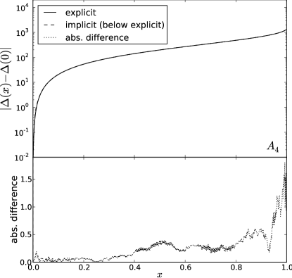
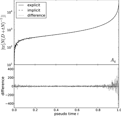
Figure 2: The integrand of Eq. 8 (lower panel) and $\Delta(x)$ (upper panel) for explicit and implicit representations of $A_{4}$.

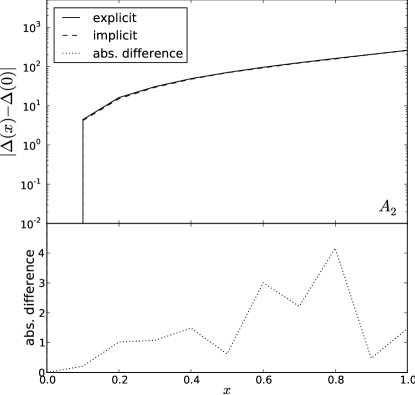
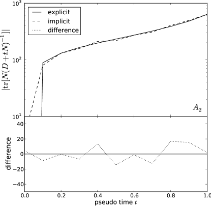
Figure 3: The integrand of Eq. 8 (lower panel) and $\Delta(x)$ (upper panel) for explicit and implicit representations of $A_{2}$ with only $m=10$ steps in pseudotime.

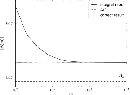
Figure 4: Dependency of the determinant’s result on the discretization of the integration interval into $m$ parts, using $A_{4}$.

II.3 Discussion

The exact numerical values of the determinant calculation using explicit and implicit representations of $A_{4}$ and $A_{2}$ can be found in Table 1. The results of the probing method (implicit) compared to the correct and the explicit method, where Eq. (8) can be evaluated without using a conjugate gradient or probing techniques, are accurate for both matrices. It is remarkable that despite using a relatively small sample size of $M=8$ the absolute errors remain relatively small. The reason for this is that the pseudotime integration over all probed integrands averages the probing error. This is of particular importance when applying the log-determinant probing to large data sets, where a large sampling size should be avoided to save computational time. These errors can be decreased further, of course, by an increase of the sampling size and a refinement of the numerical integration.

The results of the trace (integrand) probing and the determinant’s convergence behavior as well as their respective errors with respect to the explicit representation can be found in Figs. 2 and 3. Note that the scaling of the ordinate is logarithmic. For both matrices, but especially for $A_{4}$, the largest contribution to the integral of Eq. (8) comes from late $t$-values. Therefore, if dealing with big data sets, one could divide the integration interval not into $m$ equal parts but by starting with a rather coarse discretization for small $t$-values and subsequently refining it for larger values, e.g., by substituting $dt$ by $d\ln(t^{\prime})$ and thereby saving computational costs. This, however, might depend on the particular shape of the matrix and has to be studied case by case.

The dependency of the numerical value of the determinant of $A_{4}$ on the discretization (in $m$ equal parts) of the integration interval can be found in Fig. 4 and shows that even a small value of $m$ adds significant corrections to the result. The result for $m\propto\mathcal{O}(10)$ is, for instance, better than just using the determinant of the diagonal, $\Delta(0)$. This might be used in practice to investigate cheaply whether the nondiagonal structure of a matrix influences the determinant significantly.

A huge advantage of the probing method discussed here is the possibility to parallelize the numerical calculation almost completely. To be precise, the diagonal probing beforehand, the pseudotime integral, as well as every single trace probing can be parallelized fully. The only operation that cannot be parallelized is the conjugate gradient method as it is a potential minimizer, using at least the previous step to calculate the next one.

The determination of a suitable choice of the involved parameters $m$ and $M$ as well as the precision parameters for the used conjugate gradient approach and numerical integration method depend highly on the matrix to be studied. The computational costs and precision of the introduced determinant calculation thus depend on the combination of the chosen methods for diagonal and trace probing, numerical integration, the method to numerically invert the matrix $D+tN$, and the matrix $A$ itself. Since it is therefore not possible to make general statements we consciously avoid here such a discussion of computational costs and precision with respect to $m$ and $M$. A more pragmatic way to estimate these parameters would be to downscale the problem of interest until the matrix of interest fits into the memory of the computer and to subsequently perform mock tests to obtain a suitable choice for the parameters discussed above. Afterwards these values can be extrapolated to the size of the real problem.

III Applications in science

Within this section we present a selection of possible applications in science. Although there are a vast number of research fields and topics which might benefit from the stochastic estimation of a log-determinant we focus henceforth on a selection of usages in Bayesian signal inference, in particular in physics and only present simple examples. Exact, more complicated examples can be found in the cited works within this section.

III.1 Evidence calculations & model selection

The Bayesian evidence $\mathcal{P}(d)$ is a measure for the quality of the model and hence for all assumed model parameters for the data $d$ Jaynes and Bretthorst (2003). To keep it short and simple we assume a model that describes a linear measurement of a Gaussian signal $s$ with additive, signal-independent, Gaussian noise $n$, i.e.,

$$d=Rs+n,$$ (12)

where $R$ represents a linear operator. A Gaussian distribution of a variable $x$ is defined by

$$\mathcal{P}(x)=\mathcal{G}(x,X)\equiv\frac{1}{\sqrt{|2\pi X|}}\exp\left\{-\frac{1}{2}x^{\dagger}X^{-1}x\right\}$$ (13)

with related covariance matrix $X$ and mean

$$\left\langle x\right\rangle_{\mathcal{P}(x)}\equiv\int\mathcal{D}x~{}x~{}\mathcal{P}(x).$$ (14)

$\int\mathcal{D}[\cdot]$ denotes a phase space integral and $|\cdot|$ the determinant. Under these circumstances the evidence can be calculated as

$$\begin{split}\mathcal{P}(d)=&~{}\int\mathcal{D}s\int\mathcal{D}n~{}\mathcal{P}(d,s,n)\\ =&~{}\int\mathcal{D}s\int\mathcal{D}n~{}\delta(d-Rs-n)\mathcal{P}(n|s)\mathcal{P}(s)\\ =&~{}\sqrt{\frac{|2\pi C_{s|d}|}{|2\pi C_{s}||2\pi C_{n}|}}\exp\left\{-\frac{1}{2}\left(d^{\dagger}C_{n}^{-1}d-j^{\dagger}C_{s|d}j\right)\right\},\end{split}$$ (15)

with

$$\begin{split}j=&~{}R^{\dagger}C_{n}^{-1}d,\\ C^{-1}_{s|d}=&~{}R^{\dagger}C_{n}^{-1}R+C_{s}^{-1},\end{split}$$ (16)

and the signal and noise covariances $C_{s}$ and $C_{n}$, respectively. Therefore, to calculate the Bayesian model evidence, one often has to calculate determinants of covariance matrices. This might be done by probing [Eq. (8)] if dealing with implicit matrices [last line of Eq. (15)] instead of performing the multidimensional integral [second last line in Eq. (15)] numerically. The latter has been done, for instance, in the field of inflationary cosmology Planck Collaboration et al. (2014b); Martin et al. (2014) by the method of nested sampling Skilling (2004); Feroz et al. (2009).

This is especially of importance in the field of model selection or comparison Jaynes and Bretthorst (2003), where from an observation – the data – one wants to infer which theory reproduces the observation best. Switching from one model to another means, for instance, to exchange $R$ in Eq. (15), which directly affects the determinant containing $C_{s|d}$. Thus, the calculation of the determinant is mandatory here.

III.2 Posterior distribution including marginalizations

In the field of signal inference one is typically interested in reconstructing a set of $i$ parameters $p^{i}$ with uncertainty from some observation, the data $d$. This information is delivered by the posterior, given by Bayes (1763) $\mathcal{P}(p^{i}|d)\propto\mathcal{P}(d|p^{i})\mathcal{P}(p^{i})$. Often, however, this inference problem is degenerate, caused by a so-called nuisance parameter. For example, consider the calibration of an instrument is of interest and not the signal. In this case the signal $s$ represents the nuisance parameter. The common procedure to circumvent this problem is to marginalize over these parameters,

$$\mathcal{P}(p^{i}|d)\propto\int\mathcal{D}s\int\mathcal{D}n~{}\mathcal{P}(d,s,n|p^{i})\mathcal{P}(p^{i}).$$ (17)

To continue with the simple example of Sec. III.1 we assume again Gaussian distributions for $s$ and $n$ and a linear measurement but with explicit dependency on $p^{i}$, i.e., $d=(Rs)[p^{i}]+n$. If we further follow the example of calibration, the parameter $p^{i}$ might be a calibration coefficient, thus affecting only $R$. This yields $(Rs)[p^{i}]=R[p^{i}]s$ and therefore

$$\mathcal{P}(p^{i}|d)\propto\left\{\int\mathcal{D}s~{}\mathcal{G}\left(d-R[p^{i}]s,C_{n}\right)\mathcal{G}(s,C_{s})\right\}\mathcal{P}(p^{i}).$$ (18)

This integration can be performed analytically, producing an in general non-Gaussian probability distribution with $p^{i}$-dependent normalization (and exponent) similar to Eq. (15),

$$\begin{split}\mathcal{P}(p^{i}|d)\propto&~{}\sqrt{\left|2\pi C_{s|d}[p^{i}]\right|}~{}\mathcal{P}(p^{i})\\ &~{}\times\exp\left\{\frac{1}{2}j^{\dagger}[p^{i}]C_{s|d}[p^{i}]j[p^{i}]\right\}\end{split}$$ (19)

with $C_{s|d}[p^{i}]$ and $j[p^{i}]$ now containing $R[p^{i}]$ instead of $R$. In case the covariance matrices or $R[p^{i}]$ are only given by a computer routine (implicit representation of a matrix) one could use Eq. (8) to probe the determinant.

A variety of scientific fields are affected by this problem. For example, the extraction of the level of non-Gaussianity of the cosmic microwave background Dorn et al. (2013, 2014) in cosmology, the problem of self-calibration Bridle et al. (2002); Enßlin et al. (2014); Dorn et al. (2015) in general, or lensing in astronomy Hirata and Seljak (2003).

III.3 Realistic astronomical example

In order to study a more realistic example we consider a measurement device with spatially constant but unknown calibration amplitude, parametrized by $1+\gamma\in\mathds{R}$, scanning a specific patch of the sky. The measured and assumed to be Gaussian sky signal $s$ is affected by the instrument via a convolution $\mathcal{C}$ with a Gaussian kernel of standard deviation $\sigma=0.05$. Additionally, the observation might be disturbed by fore- and backgrounds. For this reason we include an observational mask $M_{o}$, which cuts out $20\%$ of the sky. The noise $n$ is still assumed to be Gaussian and uncorrelated with the signal. Hence, the measurement equation is given by

$$d=R\left[\gamma\right]s+n=(1+\gamma)M_{o}\mathcal{C}s+n.$$ (20)

To calibrate the measurement device the calibration posterior $\mathcal{P}(\gamma|d)$ has to be determined. The resulting calibration mean $\left\langle\gamma\right\rangle_{\mathcal{P}(\gamma|d)}$ can be regarded as an external calibration if the a priori knowledge on the signal is sufficiently strong. Otherwise one could infer the signal and calibration amplitude $\gamma$ simultaneously from data using iterative approaches Enßlin et al. (2014). Using Eq. (19) as well as a flat prior on $\gamma$ we obtain

$$\begin{split}\ln\mathcal{P}(\gamma|d)=&~{}-\frac{1}{2}\ln\left|C^{-1}_{s|d}\left[\gamma\right]\right|+\frac{1}{2}j^{\dagger}\left[\gamma\right]C_{s|d}\left[\gamma\right]j\left[\gamma\right]\\ &~{}+\mathrm{const}.,\end{split}$$ (21)

which exhibits in particular the $\gamma$-dependent determinant

$$\left|C^{-1}_{s|d}\left[\gamma\right]\right|=\left|(1+\gamma)~{}\mathcal{C}^{\dagger}M_{o}^{\dagger}C_{n}^{-1}M_{o}\mathcal{C}(1+\gamma)+C_{s}^{-1}\right|.$$ (22)

For the numerical evaluation of Eq. (21) we use the settings of Sec. II.2 with $C_{s}(k,k^{\prime})=\left(1+k\right)^{-3}\delta_{kk^{\prime}}$, a calibration amplitude parameter of $\gamma=2$, and a noise covariance of $\left(C_{n}\right)_{x,x^{\prime}}=10^{-1}\delta_{xx^{\prime}}$ to generate a data realization. The pseudotime interval has been discretized into $10^{2}$ parts. The numerically determined calibration posterior for a given data realization can be found in Fig. 5, which demonstrates again the efficiency of the stochastic method using only eight probes for a single trace probing operation. The figure also illustrates the impact of the determinant on the log-posterior, which would not peak in the shown interval without it.

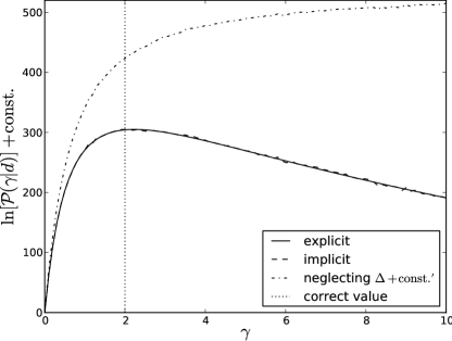
Figure 5: Logarithmic posterior of the calibration amplitude parameter $\gamma$ using implicit and explicit representations of the involved operators, see Eq. (21) and Eq. (22) for details. The abbreviation $\Delta$ denotes the logarithm of the term given by Eq. (22).

IV Summary

Motivated by the problem of finding a way to efficiently determine the determinant of an implicitly defined matrix or operator, we derived a formula, Eq. (8), representing a stochastic estimate of its log-determinant. This has been achieved by reformulating the log-determinant as an integral representation and transforming the involved terms into stochastic expressions, which includes a numerical integration and a trace probing. Numerical examples have shown that the discretization of the integration interval may be very coarse in case the probed operator is sufficiently diagonal. In case it exhibits a significant nondiagonal structure one has to fine-grain the discretization of this interval. The number of probes necessary for the trace probing, however, remains very low in the studied examples. These facts combined with the almost complete parallelizability of this approach might keep the computational costs within reasonable limits in many situations.

This method clearly has more general applications but might in particular be useful for Bayesian signal inference and model comparison when dealing with large data sets as often given, for instance, in astronomy and cosmology. To be precise, it might be beneficial in all fields where the numerical calculation of a determinant of an operator is mandatory.

Appendix A Integral representation of the log-determinant of a matrix

Here Eq. (8) is derived. Following Sec. II the log-determinant $\Delta$ of an operator $A$ can be parametrized by $\Delta=\ln[\mathrm{det}(D+N)]$ with $D$ being the diagonal and $N$ the off-diagonal part of $A$. Since $\Delta$ can be Taylor-expanded for small $N$ (spectrally compared to $D$) only, we employ a method from the field of renormalization theory Enßlin and Frommert (2011); Dorn et al. (2015). Accordingly, we introduce an expansion parameter $\delta t\ll 1$ to suppress the influence of $N$. In particular, we replace $\Delta$ by $\ln[\mathrm{det}(D+\delta tN)]$ for a moment. For sufficiently small values of $\delta t$, in the following interpreted as tiny pseudotime steps, we can approximate $\Delta$ by Eq. (6). Theoretically, a single pseudotime step could be infinitesimal small, enabling the formal definition of the derivative

$$\begin{split}\frac{d\Delta(t)}{dt}\equiv&\lim_{\delta t\rightarrow 0}\frac{\ln[\mathrm{det}(D+(t+\delta t)N)]-\ln[\mathrm{det}(D+tN)]}{\delta t}\\ =&\lim_{\delta t\rightarrow 0}~{}\frac{1}{\delta t}\ln\left[\mathrm{det}\left(\mathds{1}+\delta tN[D+tN]^{-1}\right)\right]\\ =&\lim_{\delta t\rightarrow 0}~{}\frac{1}{\delta t}\mathrm{tr}\left[\ln\left(\mathds{1}+\delta tN[D+tN]^{-1}\right)\right]\\ =&~{}\mathrm{tr}\left[N[D+tN]^{-1}\right],\end{split}$$ (23)

with the definition

$$\Delta(t)\equiv\ln[\mathrm{det}(D+tN)].$$ (24)

Integrating the pseudotime derivative of $\Delta(t)$ yields the integral representation of the log-determinant,

$$\Delta=\int_{0}^{1}dt~{}\mathrm{tr}\left[N\left(D+tN\right)^{-1}\right]+\Delta(0).$$ (25)

This integral representation has also been found by Ref. Du and Ji (2005), where its validity has been proven for weak diagonal dominant and Hermitian positive definite matrices. In particular one has to ensure the existence of the inverse matrix of the integrand of Eq. (25).

Finally, we replace the trace by stochastic trace probing and perform the pseudotime integral by an numeric integration method. This yields

$$\Delta=\int_{0}^{1}dt~{}\left\langle\xi^{\dagger}N\left(D+tN\right)^{-1}\xi\right\rangle_{\{\xi\}}+\Delta(0).$$ (26)

References

- Bennett et al. (2013) C. L. Bennett, D. Larson, J. L. Weiland, N. Jarosik, G. Hinshaw, N. Odegard, K. M. Smith, R. S. Hill, B. Gold, M. Halpern, et al., Astrophys. J. Suppl. Ser. 208, 20 (2013), eprint 1212.5225.
- Planck Collaboration et al. (2014a) Planck Collaboration, P. A. R. Ade, N. Aghanim, C. Armitage-Caplan, M. Arnaud, M. Ashdown, F. Atrio-Barandela, J. Aumont, C. Baccigalupi, A. J. Banday, et al., Astronomy and Astrophysics 571, A16 (2014a), eprint 1303.5076.
- York et al. (2000) D. G. York, J. Adelman, J. E. Anderson, Jr., S. F. Anderson, J. Annis, N. A. Bahcall, J. A. Bakken, R. Barkhouser, S. Bastian, E. Berman, et al., The Astronomical Journal 120, 1579 (2000), eprint astro-ph/0006396.
- Spergel et al. (2007) D. N. Spergel, R. Bean, O. Doré, M. R. Nolta, C. L. Bennett, J. Dunkley, G. Hinshaw, N. Jarosik, E. Komatsu, L. Page, et al., Astrophys. J. Suppl. Ser. 170, 377 (2007), eprint astro-ph/0603449.
- Hill et al. (2008) G. J. Hill, K. Gebhardt, E. Komatsu, N. Drory, P. J. MacQueen, J. Adams, G. A. Blanc, R. Koehler, M. Rafal, M. M. Roth, et al., Astronomical Society of the Pacific Conference Series 399, 115 (2008), eprint 0806.0183.
- Komatsu et al. (2005) E. Komatsu, D. N. Spergel, and B. D. Wandelt, Astrophys. J. 634, 14 (2005), eprint arXiv:astro-ph/0305189.
- Dorn et al. (2013) S. Dorn, N. Oppermann, R. Khatri, M. Selig, and T. A. Enßlin, Phys. Rev. D 88, 103516 (2013), eprint 1307.3884.
- Kitaura and Enßlin (2008) F. S. Kitaura and T. A. Enßlin, MNRAS 389, 497 (2008), eprint 0705.0429.
- Jasche and Wandelt (2013) J. Jasche and B. D. Wandelt, MNRAS 432, 894 (2013), eprint 1203.3639.
- Selig et al. (2012) M. Selig, N. Oppermann, and T. A. Enßlin, Phys. Rev. E 85, 021134 (2012), eprint 1108.0600.
- Aune et al. (2014) E. Aune, D. Simpson, and J. Eidsvik, Statistics and Computing 24, 247 (2014), ISSN 0960-3174.
- Hutchinson (1989) M. Hutchinson, Communications in Statistics - Simulation and Computation 18, 1059 (1989).
- Bekas et al. (2007) C. Bekas, E. Kokiopoulou, and Y. Saad, Applied Numerical Mathematics 57, 1214 (2007).
- Dorn et al. (2014) S. Dorn, E. Ramirez, K. E. Kunze, S. Hofmann, and T. A. Enßlin, Journal of Cosmology and Astro-Particle Physics 6, 048 (2014), eprint 1403.5067.
- Hestenes and Stiefel (1952) M. R. Hestenes and E. Stiefel, Journal of Research of the National Bureau of Standards 49, 409 (1952).
- Wu and Fitzgerald (1996) M.-D. Wu and W. Fitzgerald, Bayesian Multimodal Evidence Computation by Adapti Tempering MCMC, vol. 79 of Fundamental Theories of Physics (Springer Netherlands, 1996).
- Dickson et al. (2004) D. C. M. Dickson, M. R. Hardy, and H. R. Waters, Physics and Probability - Essays in Honor of Edwin T. Jaynes (Cambridge University Press, Cambridge, 2004), 1st ed., ISBN 978-0-521-61710-9.
- Du and Ji (2005) J. Du and J. Ji, Dynamical Systems 2005, 225 (2005).
- Selig et al. (2013) M. Selig, M. R. Bell, H. Junklewitz, N. Oppermann, M. Reinecke, M. Greiner, C. Pachajoa, and T. A. Enßlin, Astronomy and Astrophysics 554, A26 (2013), eprint 1301.4499.
- Jaynes and Bretthorst (2003) E. Jaynes and G. Bretthorst, Probability Theory: The Logic of Science, Chapter 12.4 (Cambridge University Press, 2003), ISBN 9781139435161.
- Planck Collaboration et al. (2014b) Planck Collaboration, P. A. R. Ade, N. Aghanim, C. Armitage-Caplan, M. Arnaud, M. Ashdown, F. Atrio-Barandela, J. Aumont, C. Baccigalupi, A. J. Banday, et al., Astronomy and Astrophysics 571, A22 (2014b), eprint 1303.5082.
- Martin et al. (2014) J. Martin, C. Ringeval, R. Trotta, and V. Vennin, Journal of Cosmology and Astro-Particle Physics 3, 039 (2014), eprint 1312.3529.
- Skilling (2004) J. Skilling, AIP Conference Proceedings 735, 395 (2004).
- Feroz et al. (2009) F. Feroz, M. P. Hobson, and M. Bridges, MNRAS 398, 1601 (2009), eprint 0809.3437.
- Bayes (1763) T. Bayes, Phil. Trans. of the Roy. Soc. 53, 370 (1763).
- Bridle et al. (2002) S. L. Bridle, R. Crittenden, A. Melchiorri, M. P. Hobson, R. Kneissl, and A. N. Lasenby, MNRAS 335, 1193 (2002), eprint astro-ph/0112114.
- Enßlin et al. (2014) T. A. Enßlin, H. Junklewitz, L. Winderling, M. Greiner, and M. Selig, Phys. Rev. E 90, 043301 (2014), eprint 1312.1349.
- Dorn et al. (2015) S. Dorn, T. A. Enßlin, M. Greiner, M. Selig, and V. Boehm, Phys. Rev. E 91, 013311 (2015), eprint 1410.6289.
- Hirata and Seljak (2003) C. M. Hirata and U. Seljak, Phys. Rev. D 67, 043001 (2003), eprint astro-ph/0209489.
- Enßlin and Frommert (2011) T. A. Enßlin and M. Frommert, Phys. Rev. D 83, 105014 (2011), eprint 1002.2928.