Time-causal and time-recursive spatio-temporal receptive fields

Abstract

We present an improved model and theory for time-causal and time-recursive spatio-temporal receptive fields, obtained by a combination of Gaussian receptive fields over the spatial domain and first-order integrators or equivalently truncated exponential filters coupled in cascade over the temporal domain.

Compared to previous spatio-temporal scale-space formulations in terms of non-enhancement of local extrema or scale invariance, these receptive fields are based on different scale-space axiomatics over time by ensuring non-creation of new local extrema or zero-crossings with increasing temporal scale. Specifically, extensions are presented about: (i) parameterizing the intermediate temporal scale levels, (ii) analysing the resulting temporal dynamics, (iii) transferring the theory to a discrete implementation in terms of recursive filters over time, (iv) computing scale-normalized spatio-temporal derivative expressions for spatio-temporal feature detection and (v) computational modelling of receptive fields in the lateral geniculate nucleus (LGN) and the primary visual cortex (V1) in biological vision.

We show that by distributing the intermediate temporal scale levels according to a logarithmic distribution, we obtain a new family of temporal scale-space kernels with better temporal characteristics compared to a more traditional approach of using a uniform distribution of the intermediate temporal scale levels. Specifically, the new family of time-causal kernels has much faster temporal response properties (shorter temporal delays) compared to the kernels obtained from a uniform distribution. When increasing the number of temporal scale levels, the temporal scale-space kernels in the new family do also converge very rapidly to a limit kernel possessing true self-similar scale invariant properties over temporal scales. Thereby, the new representation allows for true scale invariance over variations in the temporal scale, although the underlying temporal scale-space representation is based on a discretized temporal scale parameter.

We show how scale-normalized temporal derivatives can be defined for these time-causal scale-space kernels and how the composed theory can be used for computing basic types of scale-normalized spatio-temporal derivative expressions in a computationally efficient manner.

1 Introduction

Spatio-temporal receptive fields constitute an essential concept for describing neural functions in biological vision (Hubel and Wiesel HubWie59-Phys ; HubWie62-Phys ; HubWie05-book ; DeAngelis et al. DeAngOhzFre95-TINS ; deAngAnz04-VisNeuroSci ) and for expressing computer vision methods on video data (Adelson and Bergen AdeBer85-JOSA ; Zelnik-Manor and Irani ZelIra01-CVPR ; Laptev and Lindeberg LapLin04-ECCVWS ; Jhuang et al. JhuSerWolPog07-ICCV ; Shabani et al. ShaClaZel12-BMVC ).

For off-line processing of pre-recorded video, non-causal Gaussian or Gabor-based spatio-temporal receptive fields may in some cases be sufficient. When operating on video data in a real-time setting or when modelling biological vision computationally, one does however need to take into explicit account the fact that the future cannot be accessed and that the underlying spatio-temporal receptive fields must therefore be time-causal, i.e., the image operations should only require access to image data from the present moment and what has occurred in the past. For computational efficiency and for keeping down memory requirements, it is also desirable that the computations should be time-recursive, so that it is sufficient to keep a limited memory of the past that can be recursively updated over time.

The subject of this article is to present an improved temporal scale-space model for spatio-temporal receptive fields based on time-causal temporal scale-space kernels in terms of first-order integrators or equivalently truncated exponential filters coupled in cascade, which can be transferred to a discrete implementation in terms of recursive filters over discretized time. This temporal scale-space model will then be combined with a Gaussian scale-space concept over continuous image space or a genuinely discrete scale-space concept over discrete image space, resulting in both continuous and discrete spatio-temporal scale-space concepts for modelling time-causal and time-recursive spatio-temporal receptive fields over both continuous and discrete spatio-temporal domains. The model builds on previous work by (Fleet and Langley FleLan95-PAMI ; Lindeberg and Fagerström LF96-ECCV ; Lindeberg Lin10-JMIV ; Lin13-BICY ; Lin13-ImPhys ) and is here complemented by: (i) a better design for the degrees of freedom in the choice of time constants for the intermediate temporal scale levels from the original signal to any higher temporal scale level in a cascade structure of temporal scale-space representations over multiple temporal scales, (ii) an analysis of the resulting temporal response dynamics, (iii) details for discrete implementation in a spatio-temporal visual front-end, (iv) details for computing spatio-temporal image features in terms of scale-normalized spatio-temporal differential expressions at different spatio-temporal scales and (v) computational modelling of receptive fields in the lateral geniculate nucleus (LGN) and the primary visual cortex (V1) in biological vision.

In previous use of the temporal scale-space model in (Lindeberg and Fagerström LF96-ECCV ), a uniform distribution of the intermediate scale levels has mostly been chosen when coupling first-order integrators or equivalently truncated exponential kernels in cascade. By instead using a logarithmic distribution of the intermediate scale levels, we will here show that a new family of temporal scale-space kernels can be obtained with much better properties in terms of: (i) faster temporal response dynamics and (ii) fast convergence towards a limit kernel that possesses true scale-invariant properties (self-similarity) under variations in the temporal scale in the input data. Thereby, the new family of kernels enables: (i) significantly shorter temporal delays (as always arise for truly time-causal operations), (ii) much better computational approximation to true temporal scale invariance and (iii) computationally much more efficient numerical implementation. Conceptually, our approach is also related to the time-causal scale-time model by Koenderink Koe88-BC , which is here complemented by a truly time-recursive formulation of time-causal receptive fields more suitable for real-time operations over a compact temporal buffer of what has occurred in the past, including a theoretically well-founded and computationally efficient method for discrete implementation.

Specifically, the rapid convergence of the new family of temporal scale-space kernels to a limit kernel when the number of intermediate temporal scale levels tends to infinity is theoretically very attractive, since it provides a way to define truly scale-invariant operations over temporal variations at different temporal scales, and to measure the deviation from true scale invariance when approximating the limit kernel by a finite number of temporal scale levels. Thereby, the proposed model allows for truly self-similar temporal operations over temporal scales while using a discretized temporal scale parameter, which is a theoretically new type of construction for temporal scale spaces.

Based on a previously established analogy between scale-normalized derivatives for spatial derivative expressions and the interpretation of scale normalization of the corresponding Gaussian derivative kernels to constant $L_{p}$-norms over scale (Lindeberg Lin97-IJCV ), we will show how scale-invariant temporal derivative operators can be defined for the proposed new families of temporal scale-space kernels. Then, we will apply the resulting theory for computing basic spatio-temporal derivative expressions of different types and describe classes of such spatio-temporal derivative expressions that are invariant or covariant to basic types of natural image transformations, including independent rescaling of the spatial and temporal coordinates, illumination variations and variabilities in exposure control mechanisms.

In these ways, the proposed theory will present previously missing components for applying scale-space theory to spatio-temporal input data (video) based on truly time-causal and time-recursive image operations.

A conceptual difference between the time-causal temporal scale-space model that is developed in this paper and Koenderink’s fully continuous scale-time model Koe88-BC or the fully continuous time-causal semi-group derived by Fagerström Fag05-IJCV and Lindeberg Lin10-JMIV is that the presented time-causal scale-space model will be semi-discrete, with a continuous time axis and discretized temporal scale parameter. This semi-discrete theory can then be further discretized over time (and for spatio-temporal image data also over space) into a fully discrete theory for digital implementation. The reason why the temporal scale parameter has to be discrete in this theory is that according to theoretical results about variation-diminishing linear transformations by Schoenberg Sch30 ; Sch46 ; Sch47 ; Sch48 ; Sch50 ; Sch53 ; Sch88-book and Karlin Kar68 that we will build upon, there is no continuous parameter semi-group structure or continuous parameter cascade structure that guarantees non-creation of new structures with increasing temporal scale in terms of non-creation of new local extrema or new zero-crossings over a continuum of increasing temporal scales.

When discretizing the temporal scale parameter into a discrete set of temporal scale levels, we do however show that there exists such a discrete parameter semi-group structure in the case of a uniform distribution of the temporal scale levels and a discrete parameter cascade structure in the case of a logarithmic distribution of the temporal scale levels, which both guarantee non-creation of new local extrema or zero-crossings with increasing temporal scale. In addition, the presented semi-discrete theory allows for an efficient time-recursive formulation for real-time implementation based on a compact temporal buffer, which Koenderink’s scale-time model Koe88-BC does not, and much better temporal dynamics than the time-causal semigroup previously derived by Fagerström Fag05-IJCV and Lindeberg Lin10-JMIV .

Specifically, we argue that if the goal is to construct a vision system that analyses continuous video streams in real time, as is the main scope of this work, a restriction of the theory to a discrete set of temporal scale levels with the temporal scale levels determined in advance before the image data are sampled over time is less of a practical constraint, since the vision system anyway has to be based on a finite amount of sensors and hardware/wetware for sampling and processing the continuous stream of image data.

1.1 Structure of this article

To give the contextual overview to this work, section 2 starts by presenting a previously established computational model for spatio-temporal receptive fields in terms of spatial and temporal scale-space kernels, based on which we will replace the temporal smoothing step.

Section 3 starts by reviewing previously theoretical results for temporal scale-space models based on the assumption of non-creation of new local extrema with increasing scale, showing that the canonical temporal operators in such a model are first-order integrators or equivalently truncated exponential kernels coupled in cascade. Relative to previous applications of this idea based on a uniform distribution of the intermediate temporal scale levels, we present a conceptual extension of this idea based on a logarithmic distribution of the intermediate temporal scale levels, and show that this leads to a new family of kernels that have faster temporal response properties and correspond to more skewed distributions with the degree of skewness determined by a distribution parameter $c$.

Section 4 analyses the temporal characteristics of these kernels and shows that they lead to faster temporal characteristics in terms of shorter temporal delays, including how the choice of distribution parameter $c$ affects these characteristics. In section 5 we present a more detailed analysis of these kernels, with emphasis on the limit case when the number of intermediate scale levels $K$ tends to infinity, and making constructions that lead to true self-similarity and scale invariance over a discrete set of temporal scaling factors.

Section 6 shows how these spatial and temporal kernels can be transferred to a discrete implementation while preserving scale-space properties also in the discrete implementation and allowing for efficient computations of spatio-temporal derivative approximations. Section 7 develops a model for defining scale-normalized derivatives for the proposed temporal scale-space kernels, which also leads to a way of measuring how far from the scale-invariant time-causal limit kernel a particular temporal scale-space kernel is when using a finite number $K$ of temporal scale levels.

In section 8 we combine these components for computing spatio-temporal features defined from different types of spatio-temporal differential invariants, including an analysis of their invariance or covariance properties under natural image transformations, with specific emphasis on independent scalings of the spatial and temporal dimensions, illumination variations and variations in exposure control mechanisms. Finally, section 9 concludes with a summary and discussion, including a description about relations and differences to other temporal scale-space models.

To simplify the presentation, we have put some of the theoretical analysis in the appendix. Appendix A presents a frequency analysis of the proposed time-causal scale-space kernels, including a detailed characterization of the limit case when the number of temporal scale levels $K$ tends to infinity and explicit expressions their moment (cumulant) descriptors up to order four. Appendix B presents a comparison with the temporal kernels in Koenderink’s scale-time model, including a minor modification of Koenderink’s model to make the temporal kernels normalized to unit $L_{1}$-norm and a mapping between the parameters in his model (a temporal offset $\delta$ and a dimensionless amount of smoothing $\sigma$ relative to a logarithmic time scale) and the parameters in our model (the temporal variance $\tau$, a distribution parameter $c$ and the number of temporal scale levels $K$) including graphs of similarities vs. differences between these models. Appendix C shows that for the temporal scale-space representation given by convolution with the scale-invariant time-causal limit kernel, the corresponding scale-normalized derivatives become fully scale covariant/invariant for temporal scaling transformations that correspond to exact mappings between the discrete temporal scale levels.

This paper is a much further developed version of a conference paper Lin15-SSVM presented at the SSVM 2015, with substantial additions concerning:

• the theory that implies that the temporal scales are implied to be discrete (sections 3.1-3.2),

• more detailed modelling of biological receptive fields (section 3.6),

• the construction of a truly self-similar and scale-invariant time-causal limit kernel (section 5),

• theory for implementation in terms of discrete time-causal scale-space kernels (section 6.1),

• details concerning more rotationally symmetric implementation over spatial domain (section 6.3),

• definition of scale-normalized temporal derivatives for the resulting time-causal scale-space (section 7),

• a framework for spatio-temporal feature detection based on time-causal and time-recursive spatiotemporal scale space, including scale normalization as well as covariance and invariance properties under natural image transformations and experimental results (section 8),

• a frequency analysis of the time-causal and time-recursive scale-space kernels (appendix A),

• a comparison between the presented semi-discrete model and Koenderink’s fully continuous model, including comparisons between the temporal kernels in the two models and a mapping between the parameters in our model and Koenderink’s model (appendix B) and

• a theoretical analysis of the evolution properties over scales of temporal derivatives obtained from the time-causal limit kernel, including the scaling properties of the scale normalization factors under $L_{p}$-normalization and a proof that the resulting scale-normalized derivatives become scale invariant/covariant (appendix C).

In relation to the SSVM 2015 paper, this paper therefore first shows how the presented framework applies to spatio-temporal feature detection and computational modelling of biological vision, which could not be fully described because of space limitations, and then presents important theoretical extensions in terms of theoretical properties (scale invariance) and theoretical analysis as well as other technical details that could not be included in the conference paper because of space limitations.

2 Spatio-temporal receptive fields

The theoretical structure that we start from is a general result from axiomatic derivations of a spatio-temporal scale-space based on assumptions of non-enhancement of local extrema and the existence of a continuous temporal scale parameter, which states that the spatio-temporal receptive fields should be based on spatio-temporal smoothing kernels of the form (see overviews in Lindeberg Lin10-JMIV ; Lin13-BICY ):

$$T(x_{1},x_{2},t;\;s,\tau;\;v,\Sigma)=g(x_{1}-v_{1}t,x_{2}-v_{2}t;\;s,\Sigma)\,h(t;\;\tau)$$ (1)

where

• $x=(x_{1},x_{2})^{T}$ denotes the image coordinates,

• $t$ denotes time,

• $s$ denotes the spatial scale,

• $\tau$ denotes the temporal scale,

• $v=(v_{1},v_{2})^{T}$ denotes a local image velocity,

• $\Sigma$ denotes a spatial covariance matrix determining the spatial shape of an affine Gaussian kernel $g(x;\;s,\Sigma)=\frac{1}{2\pi s\sqrt{\det\Sigma}}e^{-x^{T}\Sigma^{-1}x/2s}$,

• $g(x_{1}-v_{1}t,x_{2}-v_{2}t;\;s,\Sigma)$ denotes a spatial affine Gaussian kernel that moves with image velocity $v=(v_{1},v_{2})$ in space-time and

• $h(t;\;\tau)$ is a temporal smoothing kernel over time.

A biological motivation for this form of separability between the smoothing operations over space and time can also be obtained from the facts that (i) most receptive fields in the retina and the LGN are to a first approximation space-time separable and (ii) the receptive fields of simple cells in V1 can be either space-time separable or inseparable, where the simple cells with inseparable receptive fields exhibit receptive fields subregions that are tilted in the space-time domain and the tilt is an excellent predictor of the preferred direction and speed of motion (DeAngelis et al. DeAngOhzFre95-TINS ; deAngAnz04-VisNeuroSci ).

For simplicity, we shall here restrict the above family of affine Gaussian kernels over the spatial domain to rotationally symmetric Gaussians of different size $s$, by setting the covariance matrix $\Sigma$ to a unit matrix. We shall also mainly restrict ourselves to space-time separable receptive fields by setting the image velocity $v$ to zero.

A conceptual difference that we shall pursue is by relaxing the requirement of a semi-group structure over a continuous temporal scale parameter in the above axiomatic derivations by a weaker Markov property over a discrete temporal scale parameter. We shall also replace the previous axiom about non-creation of new image structures with increasing scale in terms of non-enhancement of local extrema (which requires a continuous scale parameter) by the requirement that the temporal smoothing process, when seen as an operation along a one-dimensional temporal axis only, must not increase the number of local extrema or zero-crossings in the signal. Then, another family of time-causal scale-space kernels becomes permissible and uniquely determined, in terms of first-order integrators or truncated exponential filters coupled in cascade.

The main topics of this paper are to handle the remaining degrees of freedom resulting from this construction about: (i) choosing and parameterizing the distribution of temporal scale levels, (ii) analysing the resulting temporal dynamics, (iii) describing how this model can be transferred to a discrete implementation over discretized time, space or both while retaining discrete scale-space properties, (iv) using the resulting theory for computing scale-normalized spatio-temporal derivative expressions for purposes in computer vision and (v) computational modelling of biological vision.

3 Time-causal temporal scale-space

When constructing a system for real-time processing of sensor data, a fundamental constraint on the temporal smoothing kernels is that they have to be time-causal. The ad hoc solution of using a truncated symmetric filter of finite temporal extent in combination with a temporal delay is not appropriate in a time-critical context. Because of computational and memory efficiency, the computations should furthermore be based on a compact temporal buffer that contains sufficient information for representing the sensor information at multiple temporal scales and computing features therefrom. Corresponding requirements are necessary in computational modelling of biological perception.

3.1 Time-causal scale-space kernels for pure temporal domain

To model the temporal component of the smoothing operation in equation (1), let us initially consider a signal $f(t)$ defined over a one-dimensional continuous temporal axis $t\in{\mathbb{R}}$. To define a one-parameter family of temporal scale-space representation from this signal, we consider a one-parameter family of smoothing kernels $h(t;\,\tau)$ where $\tau\geq 0$ is the temporal scale parameter

$$L(t;\;\tau)=(h(\cdot;\;\tau)*f(\cdot))(t;\;\tau)=\int_{u=0}^{\infty}h(u;\ \tau)\,f(t-u)\,du$$ (2)

and $L(t;\;0)=f(t)$. To formalize the requirement that this transformation must not introduce new structures from a finer to a coarser temporal scale, let us following Lindeberg Lin90-PAMI require that between any pair of temporal scale levels $\tau_{2}>\tau_{1}\geq 0$ the number of local extrema at scale $\tau_{2}$ must not exceed the number of local extrema at scale $\tau_{1}$. Let us additionally require the family of temporal smoothing kernels $h(u;\ \tau)$ to obey the following cascade relation

$$h(\cdot;\;\tau_{2})=(\Delta h)(\cdot;\;\tau_{1}\mapsto\tau_{2})*h(\cdot;\;\tau_{1})$$ (3)

between any pair of temporal scales $(\tau_{1},\tau_{2})$ with $\tau_{2}>\tau_{1}$ for some family of transformation kernels $(\Delta h)(t;\;\tau_{1}\mapsto\tau_{2})$. Note that in contrast to most other axiomatic scale-space definitions, we do, however, not impose a strict semi-group property on the kernels. The motivation for this is to make it possible to take larger scale steps at coarser temporal scales, which will give higher flexibility and enable the construction of more efficient temporal scale-space representations.

Following Lindeberg Lin90-PAMI , let us further define a scale-space kernel as a kernel that guarantees that the number of local extrema in the convolved signal can never exceed the number of local extrema in the input signal. Equivalently, this condition can be expressed in terms of the number of zero-crossings in the signal. Following Lindeberg and Fagerström LF96-ECCV , let us additionally define a temporal scale-space kernel as a kernel that both satisfies the temporal causality requirement $h(t;\;\tau)=0$ if $t<0$ and guarantees that the number of local extrema does not increase under convolution. If both the raw transformation kernels $h(u;\ \tau)$ and the cascade kernels $(\Delta h)(t;\;\tau_{1}\mapsto\tau_{2})$ are scale-space kernels, we do hence guarantee that the number of local extrema in $L(t;\;\tau_{2})$ can never exceed the number of local extrema in $L(t;\;\tau_{1})$. If the kernels $h(u;\ \tau)$ and additionally the cascade kernels $(\Delta h)(t;\;\tau_{1}\mapsto\tau_{2})$ are temporal scale-space kernels, these kernels do hence constitute natural kernels for defining a temporal scale-space representation.

3.2 Classification of scale-space kernels for continuous signals

Interestingly, the classes of scale-space kernels and temporal scale-space kernels can be completely classified based on classical results by Schoenberg and Karlin regarding the theory of variation-diminishing linear transformations. Schoenberg studied this topic in a series of papers over about 20 years (Schoenberg Sch30 ; Sch46 ; Sch47 ; Sch48 ; Sch50 ; Sch53 ; Sch88-book ) and Karlin Kar68 then wrote an excellent monograph on the topic of total positivity.

Variation diminishing transformations.

Summarizing main results from this theory in a form relevant to the construction of the scale-space concept for one-dimensional continuous signals (Lindeberg (Lin93-Dis, , section 3.5.1)), let $S^{-}(f)$ denote the number of sign changes in a function $f$

$$S^{-}(f)=\sup V^{-}(f(t_{1}),f(t_{2}),\dots,f(t_{m})),$$ (4)

where the supremum is extended over all sets $t_{1}<t_{2}<\dots<t_{J}$ ($t_{j}\in{\mathbb{R}}$), $J$ is arbitrary but finite, and $V^{-}(v)$ denotes the number of sign changes in a vector $v$. Then, the transformation

$$f_{\mbox{\scriptsize\em out}}(\eta)=\int_{\xi=-\infty}^{\infty}f_{\mbox{\scriptsize\em in}}(\eta-\xi)\,dG(\xi),$$ (5)

where $G$ is a distribution function (essentially the primitive function of a convolution kernel), is said to be variation-diminishing if

$$S^{-}(f_{\mbox{\scriptsize\em out}})\leq S^{-}(f_{\mbox{\scriptsize\em in}})$$ (6)

holds for all continuous and bounded $f_{\mbox{\scriptsize\em in}}$. Specifically, the transformation (5) is variation diminishing if and only if $G$ has a bilateral Laplace-Stieltjes transform of the form (Schoenberg Sch50 )

$$\int_{\xi=-\infty}^{\infty}e^{-s\xi}\,dG(\xi)=C\,e^{\gamma s^{2}+\delta s}\prod_{i=1}^{\infty}\frac{e^{a_{i}s}}{1+a_{i}s}\quad$$ (7)

for $-c<\mbox{Re}(s)<c$ and some $c>0$, where $C\neq 0$, $\gamma\geq 0$, $\delta$ and $a_{i}$ are real, and $\sum_{i=1}^{\infty}a_{i}^{2}$ is convergent.

Classes of continuous scale-space kernels.

Interpreted in the temporal domain, this result implies that for continuous signals there are four primitive types of linear and shift-invariant smoothing transformations; convolution with the Gaussian kernel,

$$h(\xi)=e^{-\gamma\xi^{2}},$$ (8)

convolution with the truncated exponential functions,

$$h(\xi)=\left\{\begin{array}[]{lcl}e^{-|\lambda|\xi}&&\xi\geq 0,\\ 0&&\xi<0,\end{array}\right.\quad\quad h(\xi)=\left\{\begin{array}[]{lcl}e^{|\lambda|\xi}&&\xi\leq 0,\\ 0&&\xi>0,\end{array}\right.$$ (9)

as well as trivial translation and rescaling. Moreover, it means that a shift-invariant linear transformation is variation diminishing if and only if it can be decomposed into these primitive operations.

3.3 Temporal scale-space kernels over continuous temporal domain

In the above expressions, the first class of scale-space kernels (8) corresponds to using a non-causal Gaussian scale-space concept over time, which may constitute a straightforward model for analysing pre-recorded temporal data in an offline setting where temporal causality is not critical and can be disregarded by the possibility of accessing the virtual future in relation to any pre-recorded time moment.

Adding temporal causality as a necessary requirement, and with additional normalization of the kernels to unit $L_{1}$-norm to leave a constant signal unchanged, it follows that the following family of truncated exponential kernels

$$h_{exp}(t;\;\mu_{k})=\left\{\begin{array}[]{ll}\frac{1}{\mu_{k}}e^{-t/\mu_{k}}&t\geq 0\\ 0&t<0\end{array}\right.$$ (10)

constitutes the only class of time-causal scale-space kernels over a continuous temporal domain in the sense of guaranteeing both temporal causality and non-creation of new local extrema (or equivalently zero-crossings) with increasing scale (Lindeberg Lin90-PAMI ; Lindeberg and Fagerström LF96-ECCV ). The Laplace transform of such a kernel is given by

$$H_{exp}(q;\;\mu_{k})=\int_{t=-\infty}^{\infty}h_{exp}(t;\;\mu_{k})\,e^{-qt}\,dt=\frac{1}{1+\mu_{k}q}$$ (11)

and coupling $K$ such kernels in cascade leads to a composed kernel

$$h_{composed}(\cdot;\;\mu)=*_{k=1}^{K}h_{exp}(\cdot;\;\mu_{k})$$ (12)

having a Laplace transform of the form

$$\begin{split}H_{composed}(q;\;\mu)&=\int_{t=-\infty}^{\infty}*_{k=1}^{K}h_{exp}(\cdot;\;\mu_{k})(t)\,e^{-qt}\,dt\end{split}$$

$$\begin{split}&=\prod_{k=1}^{K}\frac{1}{1+\mu_{k}q}.\end{split}$$ (13)

The composed kernel has temporal mean and variance

$$m_{K}=\sum_{k=1}^{K}\mu_{k}\quad\quad\tau_{K}=\sum_{k=1}^{K}\mu_{k}^{2}.$$ (14)

$h(t;\;\mu,K=7)$	$h_{t}(t;\;\mu,K=7)$	$h_{tt}(t;\;\mu,K=7)$
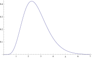
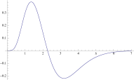
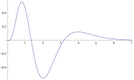
$h(t;\;K=7,c=\sqrt{2})$	$h_{t}(t;\;K=7,c=\sqrt{2}))$	$h_{tt}(t;\;K=7,c=\sqrt{2}))$
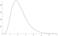
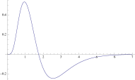
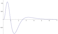
$h(t;\;K=7,c=2^{3/4})$	$h_{t}(t;\;K=7,c=2^{3/4}))$	$h_{tt}(t;\;K=7,c=2^{3/4}))$
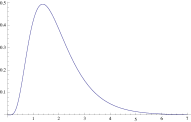
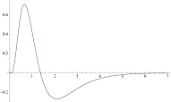
$h(t;\;K=7,c=2$	$h_{t}(t;\;K=7,c=2))$	$h_{tt}(t;\;K=7,c=2))$

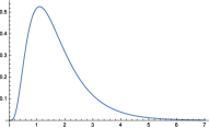
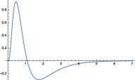
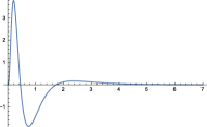
Figure 1: Equivalent kernels with temporal variance $\tau=1$ corresponding to the composition of $K=7$ truncated exponential kernels in cascade and their first- and second-order derivatives. (top row) Equal time constants $\mu$. (second row) Logarithmic distribution of the scale levels for $c=\sqrt{2}$. (third row) Logarithmic distribution for $c=2^{3/4}$. (bottom row) Logarithmic distribution for $c=2$.

In terms of physical models, repeated convolution with such kernels corresponds to coupling a series of first-order integrators with time constants $\mu_{k}$ in cascade

$$\partial_{t}L(t;\;\tau_{k})=\frac{1}{\mu_{k}}\left(L(t;\;\tau_{k-1})-L(t;\;\tau_{k})\right)$$ (15)

with $L(t;\;0)=f(t)$. In the sense of guaranteeing non-creation of new local extrema or zero-crossings over time, these kernels have a desirable and well-founded smoothing property that can be used for defining multi-scale observations over time. A constraint on this type of temporal scale-space representation, however, is that the scale levels are required to be discrete and that the scale-space representation does hence not admit a continuous scale parameter. Computationally, however, the scale-space representation based on truncated exponential kernels can be highly efficient and admits for direct implementation in terms of hardware (or wetware) that emulates first-order integration over time, and where the temporal scale levels together also serve as a sufficient time-recursive memory of the past (see figure 2).

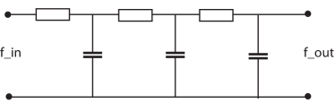
Figure 2: Electric wiring diagram consisting of a set of resistors and capacitors that emulate a series of first-order integrators coupled in cascade, if we regard the time-varying voltage $f_{in}$ as representing the time varying input signal and the resulting output voltage $f_{out}$ as representing the time varying output signal at a coarser temporal scale. According to the presented theory, the corresponding truncated exponential kernels of time are the only primitive temporal smoothing kernels that guarantee both temporal causality and non-creation of local extrema (alternatively zero-crossings) with increasing temporal scale. Such first-order temporal integration can be used as a straightforward computational model for temporal processing in biological neurons (see also Koch (Koch99-book, , Chapters 11–12) regarding physical modelling of the information transfer in dendrites of neurons).

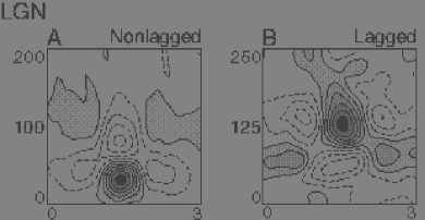
$h_{xxt}(x,t;\;s,\tau)$	$-h_{xxtt}(x,t;\;s,\tau)$

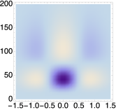
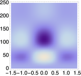
Figure 3: Computational modelling of space-time separable receptive field profiles in the lateral geniculate nucleus (LGN) as reported by DeAngelis et al. DeAngOhzFre95-TINS using idealized spatio-temporal receptive fields of the form $T(x,t;\;s,\tau)=\partial_{x^{\alpha}}\partial_{t^{\beta}}g(;\;s)\,h(t;\;\tau)$ according to equation (1) and with the temporal smoothing function $h(t;\;\tau)$ modelled as a cascade of first-order integrators/truncated exponential kernels of the form (12). (left) a “non-lagged cell” modelled using first-order temporal derivatives (right) a “lagged cell” modelled using second-order temporal derivatives. Parameter values: (a) $h_{xxt}$: $\sigma_{x}=0.5$ degrees, $\sigma_{t}=40$ ms. (b) $h_{xxtt}$: $\sigma_{x}=0.6$ degrees, $\sigma_{t}=60$ ms. (Horizontal dimension: space $x$. Vertical dimension: time $t$.)

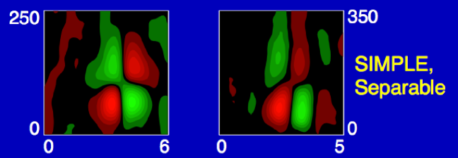
$h_{xt}(x,t;\;s,\tau)$	$-h_{xxt}(x,t;\;s,\tau)$

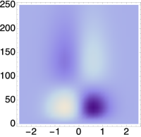
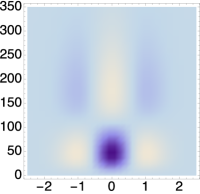
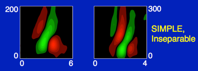
$h_{xx}(x,t;\;s,\tau,v)$	$-h_{xxx}(x,t;\;s,\tau,v)$

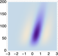
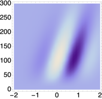
Figure 4: Computational modelling of simple cells in the primary visual cortex (V1) as reported by DeAngelis et al. DeAngOhzFre95-TINS using idealized spatio-temporal receptive fields of the form $T(x,t;\;s,\tau,v)=\partial_{x^{\alpha}}\partial_{t^{\beta}}g(x-vt;\;s)\,h(t;\;\tau)$ according to equation (1) and with the temporal smoothing function $h(t;\;\tau)$ modelled as a cascade of first-order integrators/truncated exponential kernels of the form (12). (left column) Separable receptive fields corresponding to mixed derivatives of first- or second-order derivatives over space with first-order derivatives over time. (right column) Inseparable velocity-adapted receptive fields corresponding to second- or third-order derivatives over space. Parameter values: (a) $h_{xt}$: $\sigma_{x}=0.6$ degrees, $\sigma_{t}=60$ ms. (b) $h_{xxt}$: $\sigma_{x}=0.6$ degrees, $\sigma_{t}=80$ ms. (c) $h_{xx}$: $\sigma_{x}=0.7$ degrees, $\sigma_{t}=50$ ms, $v=0.007$ degrees/ms. (d) $h_{xxx}$: $\sigma_{x}=0.5$ degrees, $\sigma_{t}=80$ ms, $v=0.004$ degrees/ms. (Horizontal axis: Space $x$ in degrees of visual angle. Vertical axis: Time $t$ in ms.)

3.4 Distributions of the temporal scale levels

When implementing this temporal scale-space concept, a set of intermediate scale levels $\tau_{k}$ has to be distributed between some minimum and maximum scale levels $\tau_{min}=\tau_{1}$ and $\tau_{max}=\tau_{K}$. Next, we will present three ways of discretizing the temporal scale parameter over $K$ temporal scale levels.

Uniform distribution of the temporal scales.

If one chooses a uniform distribution of the intermediate temporal scales

$$\tau_{k}=\frac{k}{K}\,\tau_{max}$$ (16)

then the time constants of all the individual smoothing steps are given by

$$\mu_{k}=\sqrt{\frac{\tau_{max}}{K}}.$$ (17)

Logarithmic distribution of the temporal scales with free minimum scale.

More natural is to distribute the temporal scale levels according to a geometric series, corresponding to a uniform distribution in units of effective temporal scale $\tau_{eff}=\log\tau$ (Lindeberg Lin92-PAMI ). If we have a free choice of what minimum temporal scale level $\tau_{min}$ to use, a natural way of parameterizing these temporal scale levels is by using a distribution parameter $c>1$

$$\tau_{k}=c^{2(k-K)}\tau_{max}\quad\quad(1\leq k\leq K)$$ (18)

which by equation (14) implies that time constants of the individual first-order integrators should be given by

$$\begin{split}\mu_{1}&=c^{1-K}\sqrt{\tau_{max}}\end{split}$$ (19)

$$\begin{split}\mu_{k}&=\sqrt{\tau_{k}-\tau_{k-1}}=c^{k-K-1}\sqrt{c^{2}-1}\sqrt{\tau_{max}}\quad(2\leq k\leq K)\end{split}$$ (20)

Logarithmic distribution of the temporal scales with given minimum scale.

If the temporal signal is on the other hand given at some minimum temporal scale $\tau_{min}$, we can instead determine $c=\left(\frac{\tau_{max}}{\tau_{min}}\right)^{\frac{1}{2(K-1)}}$ in (18) such that $\tau_{1}=\tau_{min}$ and add $K-1$ temporal scales with $\mu_{k}$ according to (20).

Logarithmic memory of the past.

When using a logarithmic distribution of the temporal scale levels according to either of the last two methods, the different levels in the temporal scale-space representation at increasing temporal scales will serve as a logarithmic memory of the past, with qualitative similarity to the mapping of the past onto a logarithmic time axis in the scale-time model by Koenderink Koe88-BC . Such a logarithmic memory of the past can also be extended to later stages in the visual hierarchy.

3.5 Temporal receptive fields

Figure 1 shows graphs of such temporal scale-space kernels that correspond to the same value of the composed variance, using either a uniform distribution or a logarithmic distribution of the intermediate scale levels.

In general, these kernels are all highly asymmetric for small values of $K$, whereas the kernels based on a uniform distribution of the intermediate temporal scale levels become gradually more symmetric around the temporal maximum as $K$ increases. The degree of continuity at the origin and the smoothness of transition phenomena increase with $K$ such that coupling of $K\geq 2$ kernels in cascade implies a $C^{K-2}$-continuity of the temporal scale-space kernel. To guarantee at least $C^{1}$-continuity of the temporal derivative computation kernel at the origin, the order $n$ of differentiation of a temporal scale-space kernel should therefore not exceed $K-2$. Specifically, the kernels based on a logarithmic distribution of the intermediate scale levels (i) have a higher degree of temporal asymmetry which increases with the distribution parameter $c$ and (ii) allow for faster temporal dynamics compared to the kernels based on a uniform distribution.

In the case of a logarithmic distribution of the intermediate temporal scale levels, the choice of the distribution parameter $c$ leads to a trade-off issue in that smaller values of $c$ allow for a denser sampling of the temporal scale levels, whereas larger values of $c$ lead to faster temporal dynamics and a more skewed shape of the temporal receptive fields with larger deviations from the shape of Gaussian derivatives of the same order.

3.6 Computational modelling of biological receptive fields

Receptive fields in the LGN.

Regarding visual receptive fields in the lateral geniculate nucleus (LGN), DeAngelis et al. DeAngOhzFre95-TINS ; deAngAnz04-VisNeuroSci report that most neurons (i) have approximately circular center-surround organization in the spatial domain and that (ii) most of the receptive fields are separable in space-time. There are two main classes of temporal responses for such cells: (i) a “non-lagged cell” is defined as a cell for which the first temporal lobe is the largest one (figure 3(left)), whereas (ii) a “lagged cell” is defined as a cell for which the second lobe dominates (figure 3(right)).

Such temporal response properties are typical for first- and second-order temporal derivatives of a time-causal temporal scale-space representation. For the first-order temporal derivative of a time-causal temporal scale-space kernel, the first peak is strongest, whereas the second peak may be the most dominant one for second-order temporal derivatives. The spatial response, on the other hand, shows a high similarity to a Laplacian of a Gaussian, leading to an idealized receptive field model of the form (Lindeberg (Lin13-BICY, , equation (108)))

$$h_{LGN}(x,y,t;\;s,\tau)=\pm(\partial_{xx}+\partial_{yy})\,g(x,y;\;s)\,\partial_{t^{n}}\,h(t;\;\tau).$$ (21)

Figure 3 shows results of modelling separable receptive fields in the LGN in this way, using a cascade of first-order integrators/truncated exponential kernels of the form (12) for modelling the temporal smoothing function $h(t;\;\tau)$.

Receptive fields in V1.

Concerning the neurons in the primary visual cortex (V1), DeAngelis et al. DeAngOhzFre95-TINS ; deAngAnz04-VisNeuroSci describe that their receptive fields are generally different from the receptive fields in the LGN in the sense that they are (i) oriented in the spatial domain and (ii) sensitive to specific stimulus velocities. Cells (iii) for which there are precisely localized “on” and “off” subregions with (iv) spatial summation within each subregion, (v) spatial antagonism between on- and off-subregions and (vi) whose visual responses to stationary or moving spots can be predicted from the spatial subregions are referred to as simple cells (Hubel and Wiesel HubWie59-Phys ; HubWie62-Phys ). In Lindeberg Lin13-BICY , an idealized model of such receptive fields was proposed of the form

$$\begin{split}&h_{simple-cell}(x_{1},x_{2},t;\;s,\tau,v,\Sigma)=\end{split}$$

$$\begin{split}&\quad(\cos\varphi\,\partial_{x_{1}}+\sin\varphi\,\partial_{x_{2}})^{m_{1}}(\sin\varphi\,\partial_{x_{1}}-\cos\varphi\,\partial_{x_{2}})^{m_{2}}\end{split}$$

$$\begin{split}&\quad(v_{1}\,\partial_{x_{1}}+v_{2}\,\partial_{x_{2}}+\partial_{t})^{n}\end{split}$$

$$\begin{split}&\quad g(x_{1}-v_{1}t,x_{2}-v_{2}t;\;s\,\Sigma)\,h(t;\;\tau)\end{split}$$ (22)

where

• $\partial_{\varphi}=\cos\varphi\,\partial_{x_{1}}+\sin\varphi\,\partial_{x_{2}}$ and $\partial_{\bot\varphi}=\sin\varphi\,\partial_{x_{1}}-\cos\varphi\,\partial_{x_{2}}$ denote spatial directional derivative operators in two orthogonal directions $\varphi$ and $\bot\varphi$,

• $m_{1}\geq 0$ and $m_{2}\geq 0$ denote the orders of differentiation in the two orthogonal directions in the spatial domain with the overall spatial order of differentiation $m=m_{1}+m_{2}$,

• $v_{1}\,\partial_{x_{1}}+v_{2}\,\partial_{x_{2}}+\partial_{t}$ denotes a velocity-adapted temporal derivative operator

and the meanings of the other symbols are similar as explained in connection with equation (1).

Figure 4 shows the result of modelling the spatio-temporal receptive fields of simple cells in V1 in this way, using the general idealized model of spatio-temporal receptive fields in equation (1) in combination with a temporal smoothing kernel obtained by coupling a set of first-order integrators or truncated exponential kernels in cascade. As can be seen from the figures, the proposed idealized receptive field models do well reproduce the qualitative shape of the neurophysiologically recorded biological receptive fields.

These results complement the general theoretical model for visual receptive fields in Lindeberg Lin13-BICY by (i) temporal kernels that have better temporal dynamics than the time-causal semi-group derived in Lindeberg Lin10-JMIV by decreasing faster with time (decreasing exponentially instead of polynomially) and with (ii) explicit modelling results and a theory (developed in more detail in following sections) for choosing and parameterizing the intermediate discrete temporal scale levels in the time-causal model.

With regard to a possible biological implementation of this theory, the evolution properties of the presented scale-space models over scale and time are governed by diffusion and difference equations (see equations (23)–(24) in the next section), which can be implemented by operations over neighbourhoods in combination with first-order integration over time. Hence, the computations can naturally be implemented in terms of connections between different cells. Diffusion equations are also used in mean field theory for approximating the computations that are performed by populations of neurons (Omurtag et al. OmuKniSir00-CompNeuro ; Mattia and Guidice MatGui02-PhysRevE ; Faugeras et al. FauTouCes09-FrontCompNeuroSci ).

By combination of the theoretical properties of these kernels regarding scale-space properties between receptive field responses at different spatial and temporal scales as well as their covariance properties under natural image transformations (described in more detail in the next section), the proposed theory can be seen as a both theoretically well-founded and biologically plausible model for time-causal and time-recursive spatio-temporal receptive fields.

3.7 Theoretical properties of time-causal spatio-temporal scale-space

Under evolution of time and with increasing spatial scale, the corresponding time-causal spatio-temporal scale-space representation generated by convolution with kernels of the form (1) with specifically the temporal smoothing kernel $h(t;\;\tau)$ defined as a set of truncated exponential kernels/first-order integrators in cascade (12) obeys the following system of differential/difference equations

$$\begin{split}\partial_{s}L&=\frac{1}{2}\nabla_{x}^{T}(\Sigma\,\nabla_{x}L),\end{split}$$ (23)

$$\begin{split}\partial_{t}L&=-v^{T}(\nabla_{x}L)-\frac{1}{\mu_{k}}\delta_{\tau}L,\end{split}$$ (24)

with the difference operator $\delta_{\tau}$ over temporal scale

$$(\delta_{\tau}L)(x,t;\;s,\tau_{k};\;\Sigma,v)=\\ L(x,t;\;s,\tau_{k};\;\Sigma,v)-L(x,t;\;s,\tau_{k-1};\;\Sigma,v).$$ (25)

Theoretically, the resulting spatio-temporal scale-space representation obeys similar scale-space properties over the spatial domain as the two other spatio-temporal scale-space models derived in Lindeberg Lin10-JMIV ; Lin13-BICY ; Lin13-ImPhys regarding (i) linearity over the spatial domain, (ii) shift invariance over space, (iii) semi-group and cascade properties over spatial scales, (iv) self-similarity and scale covariance over spatial scales so that for any uniform scaling transformation $(x^{\prime},t^{\prime})^{T}=(Sx,t)^{T}$ the spatio-temporal scale-space representations are related by $L^{\prime}(x^{\prime},t^{\prime};\;s^{\prime},\tau_{k};\;\Sigma,v^{\prime})=L(x,t;\;s,\tau_{k};\;\Sigma,v)$ with $s^{\prime}=S^{2}s$ and $v^{\prime}=Sv$ and (v) non-enhancement of local extrema with increasing spatial scale.

If the family of receptive fields in equation (1) is defined over the full group of positive definite spatial covariance matrices $\Sigma$ in the spatial affine Gaussian scale-space Lin93-Dis ; LG96-IVC ; Lin10-JMIV , then the receptive field family also obeys (vi) closedness and covariance under time-independent affine transformations of the spatial image domain, $(x^{\prime},t^{\prime})^{T}=(Ax,t)^{T}$ implying $L^{\prime}(x^{\prime},t^{\prime};\;s,\tau_{k};\;\Sigma^{\prime},v^{\prime})=L(x,t;\;s,\tau_{k};\;\Sigma,v)$ with $\Sigma^{\prime}=A\Sigma A^{T}$ and $v^{\prime}=Av$, and as resulting from e.g. local linearizations of the perspective mapping (with locality defined as over the support region of the receptive field). When using rotationally symmetric Gaussian kernels for smoothing, the corresponding spatio-temporal scale-space representation does instead obey (vii) rotational invariance.

Over the temporal domain, convolution with these kernels obeys (viii) linearity over the temporal domain, (ix) shift invariance over the temporal domain, (x) temporal causality, (xi) cascade property over temporal scales, (xii) non-creation of local extrema for any purely temporal signal. If using a uniform distribution of the intermediate temporal scale levels, the spatio-temporal scale-space representation obeys a (xiii) semi-group property over discrete temporal scales. Due to the finite number of discrete temporal scale levels, the corresponding spatio-temporal scale-space representation cannot however for general values of the time constants $\mu_{k}$ obey full self-similarity and scale covariance over temporal scales. Using a logarithmic distribution of the temporal scale levels and an additional limit case construction to the infinity, we will however show in section 5 that it is possible to achieve (xiv) self-similarity (41) and scale covariance (49) over the discrete set of temporal scaling transformations $(x^{\prime},t^{\prime})^{T}=(x,c^{j}t)^{T}$ that precisely corresponds to mappings between any pair of discretized temporal scale levels as implied by the logarithmically distributed temporal scale parameter with distribution parameter $c$.

Over the composed spatio-temporal domain, these kernels obey (xv) positivity and (xvi) unit normalization in $L_{1}$-norm. The spatio-temporal scale-space representation also obeys (xvii) closedness and covariance under local Galilean transformations in space-time, in the sense that for any Galilean transformation $(x^{\prime},t^{\prime})^{T}=(x-ut,t)^{T}$ with two video sequences related by $f^{\prime}(x^{\prime},t^{\prime})=f(x,t)$ their corresponding spatio-temporal scale-space representations will be equal for corresponding parameter values $L^{\prime}(x^{\prime},t^{\prime};\;s,\tau_{k};\;\Sigma,v^{\prime})=L(x,t;\;s,\tau_{k};\;\Sigma,v)$ with $v^{\prime}=v-u$.

If additionally the velocity value $v$ and/or the spatial covariance matrix $\Sigma$ can be adapted to the local image structures in terms of Galilean and/or affine invariant fixed point properties Lin10-JMIV ; LinAkbLap04-ICPR ; Lin93-Dis ; LG96-IVC , then the spatio-temporal receptive field responses can additionally be made (xviii) Galilean invariant and/or (xix) affine invariant.

4 Temporal dynamics of the time-causal kernels

For the time-causal filters obtained by coupling truncated exponential kernels in cascade, there will be an inevitable temporal delay depending on the time constants $\mu_{k}$ of the individual filters. A straightforward way of estimating this delay is by using the additive property of mean values under convolution $m_{K}=\sum_{k=1}^{K}\mu_{k}$ according to (14). In the special case when all the time constants are equal $\mu_{k}=\sqrt{\tau/K}$, this measure is given by

$$m_{uni}=\sqrt{K\tau}$$ (26)

showing that the temporal delay increases if the temporal smoothing operation is divided into a larger number of smaller individual smoothing steps.

In the special case when the intermediate temporal scale levels are instead distributed logarithmically according to (18), with the individual time constants given by (19) and (20), this measure for the temporal delay is given by

$$\begin{split}m_{log}&=\frac{c^{-K}\left(c^{2}-\left(\sqrt{c^{2}-1}+1\right)c+\sqrt{c^{2}-1}\,c^{K}\right)}{c-1}\,\sqrt{\tau}\end{split}$$ (27)

with the limit value

$$m_{log-limit}=\lim_{K\rightarrow\infty}m_{log}=\sqrt{\frac{c+1}{c-1}}\sqrt{\tau}$$ (28)

when the number of filters tends to infinity.

By comparing equations (26) and (27), we can specifically note that with increasing number of intermediate temporal scale levels a logarithmic distribution of the intermediate scales implies shorter temporal delays than a uniform distribution of the intermediate scales.

Table 2 shows numerical values of these measures for different values of $K$ and $c$. As can be seen, the logarithmic distribution of the intermediate scales allows for significantly faster temporal dynamics than a uniform distribution.

Temporal mean values $m$ of time-causal kernels
$K$	$m_{uni}$	$m_{log}$ ($c=\sqrt{2}$)	$m_{log}$ ($c=2^{3/4}$)	$m_{log}$ ($c=2$)
2	1.414	1.414	1.399	1.366
3	1.732	1.707	1.636	1.549
4	2.000	1.914	1.777	1.641
5	2.236	2.061	1.860	1.686
6	2.449	2.164	1.910	1.709
7	2.646	2.237	1.940	1.721
8	2.828	2.289	1.957	1.726
9	3.000	2.326	1.968	1.729
10	3.162	2.352	1.974	1.730
11	3.317	2.370	1.978	1.731
12	3.464	2.383	1.980	1.732

Table 1: Numerical values of the temporal delay in terms of the temporal mean $m=\sum_{k=1}^{K}\mu_{k}$ in units of $\sigma=\sqrt{\tau}$ for time-causal kernels obtained by coupling $K$ truncated exponential kernels in cascade in the cases of a uniform distribution of the intermediate temporal scale levels $\tau_{k}=k\tau/K$ or a logarithmic distribution $\tau_{k}=c^{2(k-K)}\tau$.

Temporal delays $t_{max}$ from the maxima of time-causal kernels
$K$	$t_{uni}$	$t_{log}$ ($c=\sqrt{2}$)	$t_{log}$ ($c=2^{3/4}$)	$t_{log}$ ($c=2$)
2	0.707	0.707	0.688	0.640
3	1.154	1.122	1.027	0.909
4	1.500	1.385	1.199	1.014
5	1.789	1.556	1.289	1.060
6	2.041	1.669	1.340	1.083
7	2.268	1.745	1.370	1.095
8	2.475	1.797	1.388	1.100
9	2.667	1.834	1.398	1.103
10	2.846	1.860	1.404	1.104
11	3.015	1.879	1.408	1.105
12	3.175	1.892	1.410	1.106

Table 2: Numerical values for the temporal delay of the local maximum in units of $\sigma=\sqrt{\tau}$ for time-causal kernels obtained by coupling $K$ truncated exponential kernels in cascade in the cases of a uniform distribution of the intermediate temporal scale levels $\tau_{k}=k\tau/K$ or a logarithmic distribution $\tau_{k}=c^{2(k-K)}\tau$ with $c>1$.

Additional temporal characteristics.

Because of the asymmetric tails of the time-causal temporal smoothing kernels, temporal delay estimation by the mean value may however lead to substantial overestimates compared to e.g. the position of the local maximum. To provide more precise characteristics, let us first consider the case of a uniform distribution of the intermediate temporal scales, for which a compact closed form expression is available for the composed kernel and corresponding to the probability density function of the Gamma distribution

$$h_{composed}(t;\;\mu,K)=\frac{t^{K-1}\,e^{-t/\mu}}{\mu^{K}\,\Gamma(K)}.$$ (29)

The temporal derivatives of these kernels relate to Laguerre functions (Laguerre polynomials $p_{n}^{\alpha}(t)$ multiplied by a truncated exponential kernel) according to Rodrigues formula:

$$p_{n}^{\alpha}(t)\,e^{-t}=\frac{t^{-\alpha}}{n!}\,\partial_{t}^{n}(t^{n+\alpha}e^{-t}).$$ (30)

Let us differentiate the temporal smoothing kernel

$$\partial_{t}\left(h_{composed}(t;\;\mu,K)\right)=\frac{e^{-\frac{t}{\mu}}((K-1)\mu-t)\left(\frac{t}{\mu}\right)^{K+1}}{t^{3}\,\Gamma(K)}$$ (31)

and solve for the position of the local maximum

$$\begin{split}t_{max,uni}&=(K-1)\,\mu=\frac{(K-1)}{\sqrt{K}}\sqrt{\tau}.\end{split}$$ (32)

Table 2 shows numerical values for the position of the local maximum for both types of time-causal kernels. As can be seen from the data, the temporal response properties are significantly faster for a logarithmic distribution of the intermediate scale levels compared to a uniform distribution and the difference increases rapidly with $K$. These temporal delay estimates are also significantly shorter than the temporal mean values, in particular for the logarithmic distribution.

If we consider a temporal event that occurs as a step function over time (e.g. a new object appearing in the field of view) and if the time of this event is estimated from the local maximum over time in the first-order temporal derivative response, then the temporal variation in the response over time will be given by the shape of the temporal smoothing kernel. The local maximum over time will occur at a time delay equal to the time at which the temporal kernel has its maximum over time. Thus, the position of the maximum over time of the temporal smoothing kernel is highly relevant for quantifying the temporal response dynamics.

5 The scale-invariant time-causal limit kernel

In this section, we will show that in the case of a logarithmic distribution of the intermediate temporal scale levels it is possible to extend the previous temporal scale-space concept into a limit case that permits for covariance under temporal scaling transformations, corresponding to closedness of the temporal scale-space representation to a compression or stretching of the temporal scale axis by any integer power of the distribution parameter $c$.

Concerning the need for temporal scale invariance of a temporal scale-space representation, let us first note that one could possibly first argue that the need for temporal scale invariance in a temporal scale-space representation is different from the need for spatial scale invariance in a spatial scale-space representation. Spatial scaling transformations always occur because of perspective scaling effects caused by variations in the distances between objects in the world and the observer and do therefore always need to be handled by a vision system, whereas the temporal scale remains unaffected by the perspective mapping from the scene to the image.

Temporal scaling transformations are, however, nevertheless important because of physical phenomena or spatio-temporal events occurring faster or slower. This is analogous to another source of scale variability over the spatial domain, caused by objects in the world having different physical size. To handle such scale variabilities over the temporal domain, it is therefore desirable to develop temporal scale-space concepts that allow for temporal scale invariance.

Fourier transform of temporal scale-space kernel.

When using a logarithmic distribution of the intermediate scale levels (18), the time constants of the individual first-order integrators are given by (19) and (20). Thus, the explicit expression for the Fourier transform obtained by setting $q=i\omega$ in the expression (11) is of the form

$$\hat{h}_{exp}(\omega;\;\tau,c,K)=\\ \frac{1}{1+i\,c^{1-K}\sqrt{\tau}\,\omega}\prod_{k=2}^{K}\frac{1}{1+i\,c^{k-K-1}\sqrt{c^{2}-1}\sqrt{\tau}\,\omega}.$$ (33)

Characterization in terms of temporal moments.

Although the explicit expression for the composed time-causal kernel may be somewhat cumbersome to handle for any finite number of $K$, in appendix A.1 we show how one based on a Taylor expansion of the Fourier transform can derive compact closed-form moment or cumulant descriptors of these time-causal scale-space kernels. Specifically, the limit values of the first-order moment $M_{1}$ and the higher-order central moments up to order four when the number of temporal scale levels $K$ tends to infinity are given by

$$\begin{split}\lim_{K\rightarrow\infty}M_{1}&=\sqrt{\frac{c+1}{c-1}}\,\tau^{1/2}\end{split}$$ (34)

$$\begin{split}\lim_{K\rightarrow\infty}M_{2}&=\tau\end{split}$$ (35)

$$\begin{split}\lim_{K\rightarrow\infty}M_{3}&=\frac{2(c+1)\sqrt{c^{2}-1}\,\tau^{3/2}}{\left(c^{2}+c+1\right)}\end{split}$$ (36)

$$\begin{split}\lim_{K\rightarrow\infty}M_{4}&=\frac{3\left(3c^{2}-1\right)\tau^{2}}{c^{2}+1}\end{split}$$ (37)

and give a coarse characterization of the limit behaviour of these kernels essentially corresponding to the terms in a Taylor expansion of the Fourier transform up to order four. Following a similar methodology, explicit expressions for higher-order moment descriptors can also be derived in an analogous fashion, from the Taylor coefficients of higher order, if needed for special purposes.

In figure 9 in appendix A.1 we show graphs of the corresponding skewness and kurtosis measures as function of the distribution parameter $c$, showing that both these measures increase with the distribution parameter $c$. In figure 12 in appendix B we provide a comparison between the behaviour of this limit kernel and the temporal kernel in Koenderink’s scale-time model showing that although the temporal kernels in these two models to a first approximation share qualitatively coarsely similar properties in terms of their overall shape (see figure 11 in appendix B), the temporal kernels in these two models differ significantly in terms of their skewness and kurtosis measures.

The limit kernel.

By letting the number of temporal scale levels $K$ tend to infinity, we can define a limit kernel $\Psi(t;\;\tau,c)$ via the limit of the Fourier transform (33) according to (and with the indices relabelled to better fit the limit case):

$$\begin{split}\hat{\Psi}(\omega;\;\tau,c)&=\lim_{K\rightarrow\infty}\hat{h}_{exp}(\omega;\;\tau,c,K)\end{split}$$

$$\begin{split}&=\prod_{k=1}^{\infty}\frac{1}{1+i\,c^{-k}\sqrt{c^{2}-1}\sqrt{\tau}\,\omega}.\end{split}$$ (38)

By treating this limit kernel as an object by itself, which will be well-defined because of the rapid convergence by the summation of variances according to a geometric series, interesting relations can be expressed between the temporal scale-space representations

$$L(t;\;\tau,c)=\int_{u=0}^{\infty}\Psi(u;\;\tau,c)\,f(t-u)\,du$$ (39)

obtained by convolution with this limit kernel.

Self-similar recurrence relation for the limit kernel over temporal scales.

Using the limit kernel, an infinite number of discrete temporal scale levels is implicitly defined given the specific choice of one temporal scale $\tau=\tau_{0}$:

$$\dots\frac{\tau_{0}}{c^{6}},\frac{\tau_{0}}{c^{4}},\frac{\tau_{0}}{c^{2}},\tau_{0},c^{2}\tau_{0},c^{4}\tau_{0},c^{6}\tau_{0},\dots$$ (40)

Directly from the definition of the limit kernel, we obtain the following recurrence relation between adjacent scales:

$$\Psi(\cdot;\;\tau,c)=h_{exp}(\cdot;\;\tfrac{\sqrt{c^{2}-1}}{c}\sqrt{\tau})*\Psi(\cdot;\;\tfrac{\tau}{c^{2}},c)$$ (41)

and in terms of the Fourier transform:

$$\hat{\Psi}(\omega;\;\tau,c)=\frac{1}{1+i\,\tfrac{\sqrt{c^{2}-1}}{c}\sqrt{\tau}\,\omega}\,\hat{\Psi}(\omega;\;\tfrac{\tau}{c^{2}},c).$$ (42)

Behaviour under temporal rescaling transformations.

From the Fourier transform of the limit kernel (LABEL:eq-FT-comp-kern-log-distr-limit), we can observe that for any temporal scaling factor $S$ it holds that

$$\hat{\Psi}(\tfrac{\omega}{S};\;S^{2}\tau,c)=\hat{\Psi}(\omega;\;\tau,c).$$ (43)

Thus, the limit kernel transforms as follows under a scaling transformation of the temporal domain:

$$S\,\Psi(S\,t;\;S^{2}\tau,c)=\Psi(t;\;\tau,c).$$ (44)

If we for a given choice of distribution parameter $c$ rescale the input signal $f$ by a scaling factor $S=1/c$ such that $t^{\prime}=t/c$, it then follows that the scale-space representation of $f^{\prime}$ at temporal scale $\tau^{\prime}=\tau/c^{2}$

$$L^{\prime}(t^{\prime};\;\tfrac{\tau}{c^{2}},c)=(\Psi(\cdot;\;\tfrac{\tau}{c^{2}},c)*f^{\prime}(\cdot))(t^{\prime};\;\tfrac{\tau}{c^{2}},c)$$ (45)

will be equal to the temporal scale-space representation of the original signal $f$ at scale $\tau$

$$L^{\prime}(t^{\prime};\;\tau^{\prime},c)=L(t;\;\tau,c).$$ (46)

Hence, under a rescaling of the original signal by a scaling factor $c$, a rescaled copy of the temporal scale-space representation of the original signal can be found at the next lower discrete temporal scale relative to the temporal scale-space representation of the original signal.

Applied recursively, this result implies that the temporal scale-space representation obtained by convolution with the limit kernel obeys a closedness property over all temporal scaling transformations $t^{\prime}=c^{j}t$ with temporal rescaling factors $S=c^{j}$ ($j\in{\mathbb{Z}}$) that are integer powers of the distribution parameter $c$,

$$L^{\prime}(t^{\prime};\;\tau^{\prime},c)=L(t;\;\tau,c)\quad\mbox{for}\quad t^{\prime}=c^{j}t\quad\mbox{and}\quad\tau^{\prime}=c^{2j}\tau,$$ (47)

allowing for perfect scale invariance over the restricted subset of scaling factors that precisely matches the specific set of discrete temporal scale levels that is defined by a specific choice of the distribution parameter $c$. Based on this desirable and highly useful property, it is natural to refer to the limit kernel as the scale invariant time-causal limit kernel.

Applied to the spatio-temporal scale-space representation defined by convolution with a velocity-adapted affine Gaussian kernel $g(x-vt;\;s,\Sigma)$ over space and the limit kernel $\Psi(t;\;\tau,c)$ over time

$$L(x,t;\;s,\tau,c;\;\Sigma,v)=\\ \int_{\eta\in{\mathbb{R}}^{2}}\int_{\zeta=0}^{\infty}g(\eta-v\zeta;\;s,\Sigma)\,\Psi(\zeta;\;\tau,c)\,f(x-\eta,t-\zeta)\,d\eta\,d\zeta,$$ (48)

the corresponding spatio-temporal scale-space representation will then under a scaling transformation of time $(x^{\prime},t^{\prime})^{T}=(x,c^{j}t)^{T}$ obey the closedness property

$$L^{\prime}(x^{\prime},t^{\prime};\;s,\tau^{\prime},c;\;\Sigma,v^{\prime})=L(x,t;\;s,\tau,c;\;\Sigma,v)$$ (49)

with $\tau^{\prime}=c^{2j}\tau$ and $v^{\prime}=v/c^{j}$.

Self-similarity and scale invariance of the limit kernel.

Combining the recurrence relations of the limit kernel with its transformation property under scaling transformations, it follows that the limit kernel can be regarded as truly self-similar over scale in the sense that: (i) the scale-space representation at a coarser temporal scale (here $\tau$) can be recursively computed from the scale-space representation at a finer temporal scale (here $\tau/c^{2}$) according to (41), (ii) the representation at the coarser temporal scale is derived from the input in a functionally similar way as the representation at the finer temporal scale and (iii) the limit kernel and its Fourier transform are transformed in a self-similar way (44) and (43) under scaling transformations.

In these respects, the temporal receptive fields arising from temporal derivatives of the limit kernel share structurally similar mathematical properties as continuous wavelets (Daubechies Dau92-book ; Heil and Walnut HeiWal99-SIAM ; Mallat Mal99-book ; Misiti et al. MisMisOppPog07-book ) and fractals (Mandelbrot Man82-book ; Barnsley Bar88-BOOK ; Barnsley and Rising BarRis93-book ), while with the here conceptually novel extension that the scaling behaviour and self-similarity over scale is achieved over a time-causal and time-recursive temporal domain.

6 Computational implementation

The computational model for spatio-temporal receptive fields presented here is based on spatio-temporal image data that are assumed to be continuous over time. When implementing this model on sampled video data, the continuous theory must be transferred to discrete space and discrete time.

In this section we describe how the temporal and spatio-temporal receptive fields can be implemented in terms of corresponding discrete scale-space kernels that possess scale-space properties over discrete spatio-temporal domains.

6.1 Classification of scale-space kernels for discrete signals

In section 3.2, we described how the class of continuous scale-space kernels over a one-dimensional domain can be classified based on classical results by Schoenberg regarding the theory of variation-diminishing transformations as applied to the construction of discrete scale-space theory in Lindeberg Lin90-PAMI (Lin93-Dis, , section 3.3). To later map the temporal smoothing operation to theoretically well-founded discrete scale-space kernels, we shall in this section describe corresponding classification result regarding scale-space kernels over a discrete temporal domain.

Variation diminishing transformations.

Let $v=(v_{1},v_{2},\dots,v_{n})$ be a vector of $n$ real numbers and let $V^{-}(v)$ denote the (minimum) number of sign changes obtained in the sequence $v_{1},v_{2},\dots,v_{n}$ if all zero terms are deleted. Then, based on a result by Schoenberg Sch48 the convolution transformation

$$f_{\mbox{\scriptsize\em out}}(t)=\sum_{n=-\infty}^{\infty}c_{n}f_{\mbox{\scriptsize\em in}}(t-n)$$ (50)

is variation-diminishing i.e.

$$V^{-}(f_{\mbox{\scriptsize\em out}})\leq V^{-}(f_{\mbox{\scriptsize\em in}})$$ (51)

holds for all $f_{\mbox{\scriptsize\em in}}$ if and only if the generating function of the sequence of filter coefficients $\varphi(z)=\sum_{n=-\infty}^{\infty}c_{n}z^{n}$ is of the form

$$\varphi(z)=c\;z^{k}\;e^{(q_{-1}z^{-1}+q_{1}z)}\prod_{i=1}^{\infty}\frac{(1+\alpha_{i}z)(1+\delta_{i}z^{-1})}{(1-\beta_{i}z)(1-\gamma_{i}z^{-1})}$$ (52)

where $c>0$, $k\in{\mathbb{Z}}$, $q_{-1},q_{1},\alpha_{i},\beta_{i},\gamma_{i},\delta_{i}\geq 0$ and $\sum_{i=1}^{\infty}(\alpha_{i}+\beta_{i}+\gamma_{i}+\delta_{i})<\infty$. Interpreted over the temporal domain, this means that besides trivial rescaling and translation, there are three basic classes of discrete smoothing transformations:

• two-point weighted average or generalized binomial smoothing

  $$\begin{split}f_{\mbox{\scriptsize\em out}}(x)&=f_{\mbox{\scriptsize\em in}}(x)+\alpha_{i}\,f_{\mbox{\scriptsize\em in}}(x-1)\quad(\alpha_{i}\geq 0),\\ f_{out}(x)&=f_{\mbox{\scriptsize\em in}}(x)+\delta_{i}\,f_{\mbox{\scriptsize\em in}}(x+1)\quad(\delta_{i}\geq 0),\end{split}$$ (53)

• moving average or first-order recursive filtering

  $$\begin{split}f_{\mbox{\scriptsize\em out}}(x)&=f_{\mbox{\scriptsize\em in}}(x)+\beta_{i}\,f_{\mbox{\scriptsize\em out}}(x-1)\quad(0\leq\beta_{i}<1),\\ f_{\mbox{\scriptsize\em out}}(x)&=f_{\mbox{\scriptsize\em in}}(x)+\gamma_{i}\,f_{\mbox{\scriptsize\em out}}(x+1)\quad(0\leq\gamma_{i}<1),\end{split}$$ (54)

• infinitesimal smoothing or diffusion as arising from the continuous semi-groups made possible by the factor
  $e^{(q_{-1}z^{-1}+q_{1}z)}$.

To transfer the continuous first-order integrators derived in section 3.3 to a discrete implementation, we shall in this treatment focus on the first-order recursive filters, which by additional normalization constitute both the discrete correspondence and a numerical approximation of time-causal and time-recursive first-order temporal integration (15).

6.2 Discrete temporal scale-space kernels based on recursive filters

Given video data that has been sampled by some temporal frame rate $r$, the temporal scale $\sigma_{t}$ in the continuous model in units of seconds is first transformed to a variance $\tau$ relative to a unit time sampling

$$\tau=r^{2}\,\sigma_{t}^{2}$$ (55)

where $r$ may typically be either 25 fps or 50 fps. Then, a discrete set of intermediate temporal scale levels $\tau_{k}$ is defined by (18) or (16) with the difference between successive scale levels according to $\Delta\tau_{k}=\tau_{k}-\tau_{k-1}$ (with $\tau_{0}=0$).

For implementing the temporal smoothing operation between two such adjacent scale levels (with the lower level in each pair of adjacent scales referred to as $f_{in}$ and the upper level as $f_{out}$), we make use of a first-order recursive filter normalized to the form

$$f_{out}(t)-f_{out}(t-1)=\frac{1}{1+\mu_{k}}\,(f_{in}(t)-f_{out}(t-1))$$ (56)

and having a generating function of the form

$$H_{geom}(z)=\frac{1}{1-\mu_{k}\,(z-1)}$$ (57)

which is a time-causal kernel and satisfies discrete scale-space properties of guaranteeing that the number of local extrema or zero-crossings in the signal will not increase with increasing scale (Lindeberg Lin90-PAMI ; Lindeberg and Fagerström LF96-ECCV ). These recursive filters are the discrete analogue of the continuous first-order integrators (15). Each primitive recursive filter (56) has temporal mean value $m_{k}=\mu_{k}$ and temporal variance $\Delta\tau_{k}=\mu_{k}^{2}+\mu_{k}$, and we compute $\mu_{k}$ from $\Delta\tau_{k}$ according to

$$\mu_{k}=\frac{\sqrt{1+4\Delta\tau_{k}}-1}{2}.$$ (58)

By the additive property of variances under convolution, the discrete variances of the discrete temporal scale-space kernels will perfectly match those of the continuous model, whereas the mean values and the temporal delays may differ somewhat. If the temporal scale $\tau_{k}$ is large relative to the temporal sampling density, the discrete model should be a good approximation in this respect.

By the time-recursive formulation of this temporal scale-space concept, the computations can be performed based on a compact temporal buffer over time, which contains the temporal scale-space representations at temporal scales $\tau_{k}$ and with no need for storing any additional temporal buffer of what has occurred in the past to perform the corresponding temporal operations.

Concerning the actual implementation of these operations computationally on signal processing hardware of software with built-in support for higher order recursive filtering, one can specifically note the following: If one is only interested in the receptive field response at a single temporal scale, then one can combine a set of $K^{\prime}$ first-order recursive filters (56) into a higher order recursive filter by multiplying their generating functions (57)

$$\begin{split}H_{composed}(z)&=\prod_{k=1}^{K^{\prime}}\frac{1}{1-\mu_{k}\,(z-1)}\end{split}$$

$$\begin{split}&=\frac{1}{a_{0}+a_{1}\,z+a_{2}\,z^{2}+\dots+a_{K^{\prime}}\,z^{K^{\prime}}}\end{split}$$ (59)

thus performing $K^{\prime}$ recursive filtering steps by a single call to the signal processing hardware or software. If using such an approach, it should be noted, however, that depending on the internal implementation of this functionality in the signal processing hardware/software, the composed call (LABEL:eq-gen-fcn-composed-rec-filt) may not be as numerically well-conditioned as the individual smoothing steps (56) which are guaranteed to dampen any local perturbations. In our Matlab implementation for offline processing of this receptive field model, we have therefore limited the number of compositions to $K^{\prime}=4$.

6.3 Discrete implementation of spatial Gaussian smoothing

To implement the spatial Gaussian operation on discrete sampled data, we do first transform a spatial scale parameter $\sigma_{x}$ in units of e.g. degrees of visual angle to a spatial variance $s$ relative to a unit sampling density according to

$$s=p^{2}\sigma_{x}^{2}$$ (60)

where $p$ is the number of pixels per spatial unit e.g. in terms of degrees of visual angle at the image center. Then, we convolve the image data with the separable two-dimensional discrete analogue of the Gaussian kernel (Lindeberg Lin90-PAMI )

$$T(n_{1},n_{2};\;s)=e^{-2s}I_{n_{1}}(s)\,I_{n_{2}}(s),$$ (61)

where $I_{n}$ denotes the modified Bessel functions of integer order and which corresponds to the solution of the semi-discrete diffusion equation

$$\partial_{s}L(n_{1},n_{2};\;s)=\frac{1}{2}(\nabla_{5}^{2}L)(n_{1},n_{2};\;s),$$ (62)

where $\nabla_{5}^{2}$ denotes the five-point discrete Laplacian operator defined by $(\nabla_{5}^{2}f)(n_{1},n_{2})=f(n_{1}-1,n_{2})+f(n_{1}+1,n_{2})+f(n_{1},n_{2}-1)+f(n_{1},n_{2}+1)-4f(n_{1},n_{2})$. These kernels constitute the natural way to define a scale-space concept for discrete signals corresponding to the Gaussian scale-space over a symmetric domain.

This operation can be implemented either by explicit spatial convolution with spatially truncated kernels

$$\sum_{n_{1}=-N}^{N}\sum_{n_{2}=-N}^{N}T(n_{1},n_{2};\;s)>1-\varepsilon$$ (63)

for small $\varepsilon$ of the order $10^{-8}$ to $10^{-6}$ with mirroring at the image boundaries (adiabatic boundary conditions corresponding to no heat transfer across the image boundaries) or using the closed-form expression of the Fourier transform

$$\begin{split}\varphi_{T}(\theta_{1},\theta_{2})&=\sum_{n_{1}=-\infty}^{\infty}\sum_{n_{1}=-\infty}^{\infty}T(n_{1},n_{2};\;s)\,e^{-i(n_{1}\theta_{1}+n_{2}\theta_{2})}\end{split}$$

$$\begin{split}=e^{-2t(\sin^{2}(\frac{\theta_{1}}{2})+\sin^{2}(\frac{\theta_{2}}{2}))}.\end{split}$$ (64)

Alternatively, to approximate rotational symmetry by higher degree of accuracy, one can define the 2-D spatial discrete scale-space from the solution of (Lindeberg (Lin93-Dis, , section 4.3))

$$\partial_{s}L=\frac{1}{2}\left((1-\gamma)\nabla_{5}^{2}L+\gamma\nabla_{\times^{2}}^{2}L\right),$$ (65)

where $(\nabla_{\times}^{2}f)(n_{1},n_{2})=\tfrac{1}{2}(f(n_{1}+1,n_{2}+1)+f(n_{1}+1,n_{2}-1)+f(n_{1}-1,n_{2}+1)+f(n_{1}-1,n_{2}-1)-4f(n_{1},n_{2}))$ and specifically the choice $\gamma=1/3$ gives the best approximation of rotational symmetry. In practice, this operation can be implemented by first one step of diagonal separable discrete smoothing at scale $s_{\times}=s/6$ followed by a Cartesian separable discrete smoothing at scale $s_{5}=2s/3$ or using a closed form expression for the Fourier transform derived from the difference operators

$$\varphi_{T}(\theta_{1},\theta_{2})=e^{-(2-\gamma)t+(1-\gamma)(\cos\theta_{1}+\cos\theta_{2})t+(\gamma\cos\theta_{1}\cos\theta_{2})t)}.$$ (66)

6.4 Discrete implementation of spatio-temporal receptive fields

For separable spatio-temporal receptive fields, we implement the spatio-temporal smoothing operation by separable combination of the spatial and temporal scale-space concepts in sections 6.2 and 6.3. From this representation, spatio-temporal derivative approximations are then computed from difference operators

$$\begin{split}\delta_{t}&=(-1,+1)\quad\quad\quad\delta_{tt}=(1,-2,1)\end{split}$$ (67)

$$\begin{split}\delta_{x}&=(-\frac{1}{2},0,+\frac{1}{2})\quad\quad\delta_{xx}=(1,-2,1)\end{split}$$ (68)

$$\begin{split}\delta_{y}&=(-\frac{1}{2},0,+\frac{1}{2})\quad\quad\delta_{yy}=(1,-2,1)\end{split}$$ (69)

expressed over the appropriate dimensions and with higher order derivative approximations constructed as combinations of these primitives, e.g. $\delta_{xy}=\delta_{x}\,\delta_{y}$, $\delta_{xxx}=\delta_{x}\,\delta_{xx}$, $\delta_{xxt}=\delta_{xx}\,\delta_{t}$, etc. From the general theory in (Lindeberg Lin93-JMIV ; Lin93-Dis ) it follows that the scale-space properties for the original zero-order signal will be transferred to such derivative approximations, including a true cascade smoothing property for the spatio-temporal discrete derivative approximations

$$\begin{split}L_{x_{1}^{m_{1}}x_{2}^{m_{2}}t^{n}}(x_{1},x_{2},t;\;s_{2},\tau_{k_{2}})=\end{split}$$

$$\begin{split}&=\left(\vphantom{L_{x_{1}^{m_{1}}x_{2}^{m_{2}}t^{n}}}\left(T(\cdot,\cdot;\;s_{2}-s_{1})\,(\Delta h)(\cdot;\;\tau_{k_{1}}\mapsto\tau_{k_{2}})\right)\right.*\end{split}$$

$$\begin{split}&\phantom{=\left(\right.}\left.\,\,L_{x_{1}^{m_{1}}x_{2}^{m_{2}}t^{n}}(\cdot,\cdot,\cdot;\;s_{1},\tau_{k_{1}})\right)(x_{1},x_{2},t;\;s_{2},\tau_{k_{2}}).\end{split}$$ (70)

The motivation for using symmetric differences for the first order spatial derivative approximations $\delta_{x}$ and $\delta_{y}$ is to have the derivative approximations maximally accurate at the grid points to enable straightforward combination into higher order differential invariants over image space. With this choice also certain algebraic relations that hold for derivatives of continuous Gaussian kernels will be transferred to corresponding algebraic relations for difference approximations applied to the discrete Gaussian kernel (Lindeberg (Lin93-Dis, , equations (5.34) and (5.36) at page 133)):

$$\begin{split}(\delta_{x}T)(x;\;t)&=-\frac{x}{t}\,T(x;\;t)\end{split}$$ (71)

$$\begin{split}(\delta_{xx}T)(x;\;t)&=2(\partial_{t}T)(x;\;t)\end{split}$$ (72)

The motivation for using non-symmetric first-order derivative approximations $(-1,1)$ over time is because of the temporal causality that implies the impossibility of having access to data from the future and then within this constraint minimize the temporal delay as much as possible using temporal difference operators of minimum support. Because of the non-causal temporal smoothing operation, one anyway gets an additional and much larger temporal delay that implies that all filter responses are computed with a certain and non-neglible temporal delay.

For non-separable spatio-temporal receptive fields corresponding to a non-zero image velocity $v=(v_{1},v_{2})^{T}$, we implement the spatio-temporal smoothing operation by first warping the video data $(x_{1}^{\prime},x_{2}^{\prime})^{T}=(x_{1}-v_{1}t,x_{2}-v_{2}t)^{T}$ using spline interpolation. Then, we apply separable spatio-temporal smoothing in the transformed domain and unwarp the result back to the original domain. Over a continuous domain, such an operation is equivalent to convolution with corresponding velocity-adapted spatio-temporal receptive fields, while being significantly faster in a discrete implementation than explicit convolution with non-separable receptive fields over three dimensions.

7 Scale normalization for spatio-temporal derivatives

When computing spatio-temporal derivatives at different scales, some mechanism is needed for normalizing the derivatives with respect to the spatial and temporal scales, to make derivatives at different spatial and temporal scales comparable and to enable spatial and temporal scale selection.

7.1 Scale normalization of spatial derivatives

For the Gaussian scale-space concept defined over a purely spatial domain, it can be shown that the canonical way of defining scale-normalized derivatives at different spatial scales $s$ is according to (Lindeberg Lin97-IJCV )

$$\partial_{\xi_{1}}=s^{\gamma_{s}/2}\,\partial_{x_{1}},\quad\quad\partial_{\xi_{2}}=s^{\gamma_{s}/2}\,\partial_{x_{2}},$$ (73)

where $\gamma_{s}$ is a free parameter. Specifically, it can be shown (Lindeberg (Lin97-IJCV, , section 9.1)) that this notion of $\gamma$-normalized derivatives corresponds to normalizing the $m$:th order Gaussian derivatives $g_{\xi^{m}}=g_{\xi_{1}^{m_{1}}\xi_{2}^{m_{2}}}$ in $N$-dimensional image space to constant $L_{p}$-norms over scale

$$\|g_{\xi^{m}}(\cdot;\;s)\|_{p}=\left(\int_{x\in{\mathbb{R}}^{N}}|g_{\xi^{m}}(x;\;s)|^{p}\,dx\right)^{1/p}=G_{m,\gamma_{s}}$$ (74)

with

$$p=\frac{1}{1+\frac{|m|}{N}(1-\gamma_{s})}$$ (75)

where the perfectly scale invariant case $\gamma_{s}=1$ corresponds to $L_{1}$-normalization for all orders $|m|=m_{1}+\dots+m_{N}$. In this paper, we will throughout use this approach for normalizing spatial differentiation operators with respect to the spatial scale parameter $s$.

7.2 Scale normalization of temporal derivatives

If using a non-causal Gaussian temporal scale-space concept, scale-normalized temporal derivatives can be defined in an analogous way as scale-normalized spatial derivatives as described in the previous section.

For the time-causal temporal scale-space concept based on first-order temporal integrators coupled in cascade, we can also define a corresponding notion of scale-normalized temporal derivatives

$$\partial_{\zeta^{n}}=\tau^{n\gamma_{\tau}/2}\,\partial_{t^{n}}$$ (76)

which will be referred to as variance-based normalization reflecting the fact the parameter $\tau$ corresponds to variance of the composed temporal smoothing kernel. Alternatively, we can determine a temporal scale normalization factor $\alpha_{n,\gamma_{\tau}}(\tau)$

$$\partial_{\zeta^{n}}=\alpha_{n,\gamma_{\tau}}(\tau)\,\partial_{t^{n}}$$ (77)

such that the $L_{p}$-norm (with $p$ determined as function of $\gamma$ according to (75)) of the corresponding composed scale-normalized temporal derivative computation kernel $\alpha_{n,\gamma_{\tau}}(\tau)\,h_{t^{n}}$ equals the $L_{p}$-norm of some other reference kernel, where we here initially take the $L_{p}$-norm of the corresponding Gaussian derivative kernels

$$\begin{split}\|\alpha_{n,\gamma_{\tau}}(\tau)\,h_{t^{n}}(\cdot;\;\tau)\|_{p}&=\alpha_{n,\gamma_{\tau}}(\tau)\,\|h_{t^{n}}(\cdot;\;\tau)\|_{p}\end{split}$$

$$\begin{split}&=\|g_{\xi^{n}}(\cdot;\;\tau)\|_{p}=G_{n,\gamma_{\tau}}.\end{split}$$ (78)

This latter approach will be referred to as $L_{p}$-normalization.

For the discrete temporal scale-space concept over discrete time, scale normalization factors for discrete $l_{p}$-normalization are defined in an analogous way with the only difference that the continuous $L_{p}$-norm is replaced by a discrete $l_{p}$-norm.

In the specific case when the temporal scale-space representation is defined by convolution with the scale-invariant time-causal limit kernel according to (39) and (LABEL:eq-FT-comp-kern-log-distr-limit), it is shown in appendix C that the corresponding scale-normalized derivatives become truly scale covariant under temporal scaling transformations $t^{\prime}=c^{j}t$ with scaling factors $S=c^{j}$ that are integer powers of the distribution parameter $c$

$$\begin{split}L^{\prime}_{\zeta^{\prime n}}(t^{\prime};\,\tau^{\prime},c)&=c^{jn(\gamma-1)}\,L_{\zeta^{n}}(t;\,\tau,c)\end{split}$$

$$\begin{split}&=c^{j(1-1/p)}\,L_{\zeta^{n}}(t;\,\tau,c)\end{split}$$ (79)

between matching temporal scale levels $\tau^{\prime}=c^{2j}\tau$. Specifically, for $\gamma=1$ corresponding to $p=1$ the scale-normalized temporal derivatives become fully scale invariant

$$L^{\prime}_{\zeta^{\prime n}}(t^{\prime};\,\tau^{\prime},c)=L_{\zeta^{n}}(t;\,\tau,c).$$ (80)

Temporal scale normalization factors for $n=1$ at $\tau=1$
$K$	$\tau^{n/2}$	$\alpha_{n,\gamma_{\tau}}(\tau)$ (uni)	$\alpha_{n,\gamma_{\tau}}(\tau)$ ($c=\sqrt{2}$)	$\alpha_{n,\gamma_{\tau}}(\tau)$ ($c=2^{3/4}$)	$\alpha_{n,\gamma_{\tau}}(\tau)$ ($c=2$)
2	1.000	0.744	0.744	0.737	0.723
3	1.000	0.805	0.794	0.765	0.736
4	1.000	0.847	0.814	0.771	0.737
5	1.000	0.877	0.821	0.772	0.738
6	1.000	0.901	0.823	0.772	0.738
7	1.000	0.920	0.823	0.772	0.738
8	1.000	0.935	0.823	0.772	0.738
⋮
16	1.000	0.998	0.823	0.772	0.738

Temporal scale normalization factors for $n=1$ at $\tau=16$
$K$	$\tau^{n/2}$	$\alpha_{n,\gamma_{\tau}}(\tau)$ (uni)	$\alpha_{n,\gamma_{\tau}}(\tau)$ ($c=\sqrt{2}$)	$\alpha_{n,\gamma_{\tau}}(\tau)$ ($c=2^{3/4}$)	$\alpha_{n,\gamma_{\tau}}(\tau)$ ($c=2$)
2	4.000	3.056	3.056	3.016	2.938
3	4.000	3.398	3.341	3.210	3.041
4	4.000	3.553	3.432	3.223	3.068
5	4.000	3.642	3.442	3.227	3.071
6	4.000	3.731	3.452	3.228	3.071
7	4.000	3.744	3.457	3.228	3.071
8	4.000	3.809	3.459	3.228	3.071
⋮
16	4.000	3.891	3.460	3.338	3.071

Temporal scale normalization factors for $n=1$ at $\tau=256$
$K$	$\tau^{n/2}$	$\alpha_{n,\gamma_{\tau}}(\tau)$ (uni)	$\alpha_{n,\gamma_{\tau}}(\tau)$ ($c=\sqrt{2}$)	$\alpha_{n,\gamma_{\tau}}(\tau)$ ($c=2^{3/4}$)	$\alpha_{n,\gamma_{\tau}}(\tau)$ ($c=2$)
2	16.000	12.270	12.270	12.084	11.711
3	16.000	13.612	13.420	12.835	12.147
4	16.000	14.242	13.732	12.932	12.162
5	16.000	14.610	13.815	12.930	12.155
6	16.000	14.850	13.816	12.927	12.152
7	16.000	15.018	13.817	12.922	12.151
8	16.000	15.145	13.817	12.922	12.151
⋮
16	16.000	15.583	13.816	12.922	12.151

Table 3: Numerical values of scale normalization factors for discrete temporal derivative approximations, using either variance-based normalization $\tau^{n/2}$ or $l_{p}$-normalization $\alpha_{n,\gamma_{\tau}}(\tau)$, for temporal derivatives of order $n=1$ and at temporal scales $\tau=1$, $\tau=16$ and $\tau=256$ relative to a unit temporal sampling rate with $\Delta t=1$ and with $\gamma_{\tau}=1$, for time-causal kernels obtained by coupling $K$ first-order recursive filters in cascade with either a uniform distribution of the intermediate scale levels or a logarithmic distribution for $c=\sqrt{2}$, $c=2^{3/4}$ and $c=2$.

Temporal scale normalization factors for $n=2$ at $\tau=1$
$K$	$\tau^{n/2}$	$\alpha_{n,\gamma_{\tau}}(\tau)$ (uni)	$\alpha_{n,\gamma_{\tau}}(\tau)$ ($c=\sqrt{2}$)	$\alpha_{n,\gamma_{\tau}}(\tau)$ ($c=2^{3/4}$)	$\alpha_{n,\gamma_{\tau}}(\tau)$ ($c=2$)
2	1.000	0.617	0.617	0.606	0.586
3	1.000	0.711	0.694	0.649	0.607
4	1.000	0.738	0.718	0.659	0.609
5	1.000	0.755	0.721	0.660	0.609
6	1.000	0.768	0.722	0.660	0.609
7	1.000	0.779	0.722	0.660	0.609
8	1.000	0.787	0.722	0.660	0.609
⋮
16	1.000	0.824	0.722	0.660	0.609

Temporal scale normalization factors for $n=2$ at $\tau=16$
$K$	$\tau^{n/2}$	$\alpha_{n,\gamma_{\tau}}(\tau)$ (uni)	$\alpha_{n,\gamma_{\tau}}(\tau)$ ($c=\sqrt{2}$)	$\alpha_{n,\gamma_{\tau}}(\tau)$ ($c=2^{3/4}$)	$\alpha_{n,\gamma_{\tau}}(\tau)$ ($c=2$)
2	16.000	4.622	4.622	4.472	4.172
3	16.000	8.429	8.017	6.897	5.701
4	16.000	10.184	9.160	7.885	6.208
5	16.000	11.363	9.698	7.871	6.296
6	16.000	12.241	10.022	7.864	6.305
7	16.000	12.690	10.088	7.862	6.305
8	16.000	13.106	10.068	7.862	6.305
⋮
16	16.000	14.575	10.058	7.862	6.305

Temporal scale normalization factors for $n=2$ at $\tau=256$
$K$	$\tau^{n/2}$	$\alpha_{n,\gamma_{\tau}}(\tau)$ (uni)	$\alpha_{n,\gamma_{\tau}}(\tau)$ ($c=\sqrt{2}$)	$\alpha_{n,\gamma_{\tau}}(\tau)$ ($c=2^{3/4}$)	$\alpha_{n,\gamma_{\tau}}(\tau)$ ($c=2$)
2	256.00	58.95	58.95	56.63	51.84
3	256.00	133.37	127.68	112.66	94.71
4	256.00	165.14	148.96	124.04	101.16
5	256.00	183.75	156.04	126.42	101.13
6	256.00	195.99	158.69	126.65	101.12
7	256.00	204.71	159.17	126.56	101.12
8	256.00	211.10	159.23	126.55	101.12
⋮
16	256.00	233.78	159.28	126.55	101.12

Table 4: Numerical values of scale normalization factors for discrete temporal derivative approximations, for either variance-based normalization $\tau^{n/2}$ or $l_{p}$-normalization $\alpha_{n,\gamma_{\tau}}(\tau)$, for temporal derivatives of order $n=2$ and at temporal scales $\tau=1$, $\tau=16$ and $\tau=256$ relative to a unit temporal sampling rate with $\Delta t=1$ and with $\gamma_{\tau}=1$, for time-causal kernels obtained by coupling $K$ first-order recursive filters in cascade with either a uniform distribution of the intermediate scale levels or a logarithmic distribution for $c=\sqrt{2}$, $c=2^{3/4}$ and $c=2$.

Relative deviation from limit of scale normalization factors for $n=1$ at $\tau=256$
$K$	$\varepsilon_{n}$ (uni)	$\varepsilon_{n}$ ($c=\sqrt{2}$)	$\varepsilon_{n}$ ($c=2^{3/4}$)	$\varepsilon_{n}$ ($c=2$)
2	0.233	$1.1\cdot 10^{-1}$	$6.5\cdot 10^{-2}$	$3.6\cdot 10^{-2}$
4	0.110	$6.1\cdot 10^{-3}$	$8.5\cdot 10^{-4}$	$8.6\cdot 10^{-4}$
8	0.053	$4.9\cdot 10^{-4}$	$1.1\cdot 10^{-5}$	$2.0\cdot 10^{-7}$
16	0.026	$1.2\cdot 10^{-7}$	$9.0\cdot 10^{-13}$	$1.5\cdot 10^{-15}$
32	0.013	$3.1\cdot 10^{-14}$	$2.9\cdot 10^{-14}$	$3.4\cdot 10^{-14}$

Relative deviation from limit of scale normalization factors for $n=2$ at $\tau=256$
$K$	$\varepsilon_{n}$ (uni)	$\varepsilon_{n}$ ($c=\sqrt{2}$)	$\varepsilon_{n}$ ($c=2^{3/4}$)	$\varepsilon_{n}$ ($c=2$)
2	0.770	$6.3\cdot 10^{-1}$	$5.5\cdot 10^{-1}$	$4.9\cdot 10^{-1}$
4	0.354	$6.5\cdot 10^{-2}$	$2.0\cdot 10^{-2}$	$4.1\cdot 10^{-2}$
8	0.174	$3.2\cdot 10^{-4}$	$1.3\cdot 10^{-5}$	$1.6\cdot 10^{-8}$
16	0.085	$1.8\cdot 10^{-7}$	$1.0\cdot 10^{-12}$	$9.6\cdot 10^{-15}$
32	0.042	$1.2\cdot 10^{-13}$	$6.2\cdot 10^{-14}$	$4.0\cdot 10^{-14}$

Table 5: Numerical estimates of the relative deviation from the limit case when using different numbers $K$ of temporal scale levels for a uniform vs. a logarithmic distribution of the intermediate scale levels. The deviation measure $\varepsilon_{n}$ according to equation (87) measures the relative deviation of the scale normalization factors when using a finite number $K$ of temporal scale levels compared to the limit case when the number of temporal scale levels $K$ tends to infinity. (These estimates have been computed at a coarse temporal scale $\tau=256$ relative to a unit grid spacing so that the influence of discretization effects should be small. The limit case has been approximated by $K=1000$ for the uniform distribution and $K=500$ for the logarithmic distribution.)

7.3 Computation of temporal scale normalization factors

For computing the temporal scale normalization factors

$$\alpha_{n,\gamma_{\tau}}(\tau)=\frac{\|g_{\xi^{n}}(\cdot;\;\tau)\|_{p}}{\|h_{t^{n}}(\cdot;\;\tau)\|_{p}}$$ (81)

in (77) for $L_{p}$-normalization according to (LABEL:eq-sc-norm-der-Lp-norm-2), we compute the $L_{p}$-norms of the scale-normalized Gaussian derivatives, from closed-form expressions if $\gamma=1$ (corresponding to $p=1$)

$$\begin{split}G_{1,1}&=\left.\int_{-\infty}^{\infty}|g_{\xi}(u;\;t)|\,du\right|_{\gamma=1}=\sqrt{\frac{2}{\pi}}\approx 0.797885,\end{split}$$ (82)

$$\begin{split}G_{2,1}&=\left.\int_{-\infty}^{\infty}|g_{\xi^{2}}(u;\;t)|\,du\right|_{\gamma=1}=\sqrt{\frac{8}{\pi\,e}}\approx 0.967883,\end{split}$$ (83)

$$\begin{split}G_{3,1}&=\left.\int_{-\infty}^{\infty}|g_{\xi^{3}}(u;\;t)|\,du\right|_{\gamma=1}\end{split}$$

$$\begin{split}&=\sqrt{\frac{2}{\pi}}\left(1+\frac{4}{e^{3/2}}\right)\approx 1.51003,\end{split}$$ (84)

$$\begin{split}G_{4,1}&=\left.\int_{-\infty}^{\infty}|g_{\xi^{4}}(u;\;t)|\,du\right|_{\gamma=1}\end{split}$$

$$\begin{split}&=\frac{4\sqrt{3}}{e^{3/2+\sqrt{3/2}}\,\sqrt{\pi}}(\sqrt{3-\sqrt{6}}\,e^{\sqrt{6}}+\sqrt{3+\sqrt{6}})\end{split}$$

$$\begin{split}&\approx 2.8006.\end{split}$$ (86)

or for values of $\gamma\neq 1$ by numerical integration. For computing the discrete $l_{p}$-norm of discrete temporal derivative approximations, we first (i) filter a discrete delta function by the corresponding cascade of first-order integrators to obtain the temporal smoothing kernel and then (ii) apply discrete derivative approximation operators to this kernel to obtain the corresponding equivalent temporal derivative kernel, (iii) from which the discrete $l_{p}$-norm is computed by straightforward summation.

To illustrate how the choice of temporal scale normalization method may affect the results in a discrete implementation, tables 3–4 show examples of temporal scale normalization factors computed in these ways by either (i) variance-based normalization $\tau^{n/2}$ according to (76) or (ii) $L_{p}$-normalization $\alpha_{n,\gamma_{\tau}}(\tau)$ according to (77)–(LABEL:eq-sc-norm-der-Lp-norm-2) for different orders of temporal temporal differentiation $n$, different distribution parameters $c$ and at different temporal scales $\tau$, relative to a unit temporal sampling rate. The value $c=\sqrt{2}$ corresponds to a natural minimum value of the distribution parameter from the constraint $\mu_{2}\geq\mu_{1}$, the value $c=2$ to a doubling scale sampling strategy as used in a regular spatial pyramids and $c=2^{3/4}$ to a natural intermediate value between these two. The temporal scale level $\tau=1$ is near the discrete temporal sampling rate where temporal discretization effects are strong, $\tau=16$ is a higher temporal scale where temporal sampling effects are moderate and $\tau=256$ corresponds to a temporal scale much higher than discrete temporal sampling distance and the temporal sampling effects therefore can be expected to be small.

Notably, the numerical values of the resulting scale normalization factors may differ substantially depending on the type of scale normalization method and the underlying number of first-order recursive filters that are coupled in cascade. Therefore, the choice of temporal scale normalization method warrants specific attention in applications where the relations between numerical values of temporal derivatives at different temporal scales may have critical influence.

Specifically, we can note that the temporal scale normalization factors based on $L_{p}$-normalization differ more from the scale normalization factors from variance-based normalization (i) in the case of a logarithmic distribution of the intermediate temporal scale levels compared to a uniform distribution, (ii) when the distribution parameter $c$ increases within the family of temporal receptive fields based on a logarithmic distribution of the intermediate scale levels or (iii) a very low number of recursive filters are coupled in cascade. In all three cases, the resulting temporal smoothing kernels become more asymmetric and do hence differ more from the symmetric Gaussian model.

On the other hand, with increasing values of $K$ the numerical values of the scale normalization factors converge much faster to their limit values when using a logarithmic distribution of the intermediate scale levels compared to using a uniform distribution. Depending on the value of the distribution parameter $c$, the scale normalization factors do reasonably well approach their limit values after $K=4$ to $K=8$ scale levels, whereas much larger values of $K$ would be needed if using a uniform distribution. The convergence rate is faster for larger values of $c$.

7.4 Measuring the deviation from the scale-invariant time-causal limit kernel

To quantify how good an approximation a time-causal kernel with a finite number of $K$ scale levels is to the limit case when the number of scale levels $K$ tends to infinity, let us measure the relative deviation of the scale normalization factors from the limit kernel according to

$$\varepsilon_{n}(\tau)=\frac{\left|\left.\alpha_{n}(\tau)\right|_{K}-\left.\alpha_{n}(\tau)\right|_{K\rightarrow\infty}\right|}{\left.\alpha_{n}(\tau)\right|_{K\rightarrow\infty}}.$$ (87)

Table 5 shows numerical estimates of this relative deviation measure for different values of $K$ from $K=2$ to $K=32$ for the time-causal kernels obtained from a uniform vs. a logarithmic distribution of the scale values. From the table, we can first note that the convergence rate with increasing values of $K$ is significantly faster when using a logarithmic vs. a uniform distribution of the intermediate scale levels.

Not even $K=32$ scale levels is sufficient to drive the relative deviation measure below $1~{}\%$ for a uniform distribution, whereas the corresponding deviation measures are down to machine precision when using $K=32$ levels for a logarithmic distribution. When using $K=4$ scale levels, the relative derivation measure is down to $10^{-2}$ to $10^{-4}$ for a logarithmic distribution. If using $K=8$ scale levels, the relative deviation measure is down to $10^{-4}$ to $10^{-8}$ depending on the value of the distribution parameter $c$ and the order $n$ of differentiation.

From these results, we can conclude that one should not use a too low number of recursive filters that are coupled in cascade when computing temporal derivatives. Our recommendation is to use a logarithmic distribution with a minimum of four recursive filters for derivatives up to order two at finer scales and a larger number of recursive filters at coarser scales. When performing computations at a single temporal scale, we often use $K=7$ or $K=8$ as default.

8 Spatio-temporal feature detection

In the following, we shall apply the above theoretical framework for separable time-causal spatio-temporal receptive fields for computing different types of spatio-temporal feature, defined from spatio-temporal derivatives of different spatial and temporal orders, which may additionally be combined into composed (linear or non-linear) differential expressions.

$-T(x,t;\;s,\tau)$

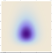
$T_{x}(x,t;\;s,\tau)$	$T_{t}(x,t;\;s,\tau,\delta)$

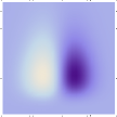
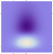
$T_{xx}(x,t;\;s,\tau)$	$T_{xt}(x,t;\;s,\tau)$	$T_{tt}(x,t;\;s,\tau)$

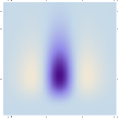
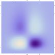
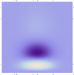
Figure 5: Space-time separable kernels $T_{x^{m}t^{n}}(x,t;\;s,\tau)=\partial_{x^{m}t^{n}}(g(x;\;s)\,h(t;\;\tau))$ up to order two obtained as the composition of Gaussian kernels over the spatial domain $x$ and a cascade of truncated exponential kernels over the temporal domain $t$ with a logarithmic distribution of the intermediate temporal scale levels ($s=1$, $\tau=1$, $K=7$, $c=\sqrt{2}$). (Horizontal axis: space $x$. Vertical axis: time $t$.)

$-T(x,t;\;s,\tau,v)$

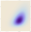
$T_{x}(x,t;\;s,\tau,v)$	$T_{t}(x,t;\;s,\tau,\delta)$

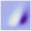
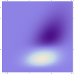
$T_{xx}(x,t;\;s,\tau,v)$	$T_{xt}(x,t;\;s,\tau,v)$	$T_{tt}(x,t;\;s,\tau,v)$

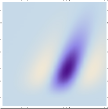
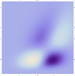
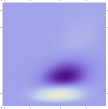
Figure 6: Velocity-adapted spatio-temporal kernels $T_{x^{m}t^{n}}(x,t;\;s,\tau,v)=\partial_{x^{m}t^{n}}(g(x-vt;\;s)\,h(t;\;\tau))$ up to order two obtained as the composition of Gaussian kernels over the spatial domain $x$ and a cascade of truncated exponential kernels over the temporal domain $t$ with a logarithmic distribution of the intermediate temporal scale levels ($s=1$, $\tau=1$, $K=7$, $c=\sqrt{2}$, $v=0.5$). (Horizontal axis: space $x$. Vertical axis: time $t$.)

8.1 Partial derivatives

A most basic approach is to first define a spatio-temporal scale-space representation $L\colon{\mathbb{R}}^{2}\times{\mathbb{R}}\times{\mathbb{R}}_{+}\times{\mathbb{R}}_{+}$ from any video data $f\colon{\mathbb{R}}^{2}\times{\mathbb{R}}$ and then defining partial derivatives of any spatial and temporal orders $m=(m_{1},m_{2})$ and $n$ at any spatial and temporal scales $s$ and $\tau$ according to

$$L_{x_{1}^{m_{1}}x_{2}^{m_{1}}t^{n}}(x_{1},x_{2},t;\;s,\tau)=\\ \partial_{x_{1}^{m_{1}}x_{2}^{m_{2}}t^{n}}\left(\left(g(\cdot,\cdot;\;s)\,h(\cdot;\;\tau)\right)*f(\cdot,\cdot,\cdot)\right)(x_{1},x_{2},t;\;s,\tau)$$ (88)

leading to a spatio-temporal $N$-jet representation of any order

$$\{L_{x},L_{y},L_{t},L_{xx},L_{xy},L_{yy},L_{xt},L_{yt},L_{tt},\dots\}.$$ (89)

Figure 6 shows such kernels up to order two in the case of a 1+1-D space-time.

8.2 Directional derivatives

By combining spatial directional derivative operators over any pair of ortogonal directions $\partial_{\varphi}=\cos\varphi\,\partial_{x}+\sin\varphi\,\partial_{y}$ and $\partial_{\bot\varphi}=\sin\varphi\,\partial_{x}-\cos\varphi\,\partial_{y}$ and velocity-adapted temporal derivatives $\partial_{t_{v}}=\partial_{t}+v_{x}\,\partial_{x}+v_{y}\,\partial_{y}$ over any motion direction $v=(v_{x},v_{y},1)$, a filter bank of spatio-temporal derivative responses can be created

$$L_{\varphi^{m_{1}}\bot\varphi^{m_{2}}t_{v}^{n}}=\partial_{\varphi}^{m_{1}}\partial_{\bot\varphi}^{m_{2}}\partial_{t_{v}}^{n}L$$ (90)

for different sampling strategies over image orientations $\varphi$ and $\bot\varphi$ in image space and over motion directions $v$ in space-time (see figure 6 for illustrations of such kernels up to order two in the case of a 1+1-D space-time).

Note that as long as the spatio-temporal smoothing operations are performed based on rotationally symmetric Gaussians over the spatial domain and using space-time separable kernels over space-time, the responses to these directional derivative operators can be directly related to corresponding partial derivative operators by mere linear combinations. If extending the rotationally symmetric Gaussian scale-space concept is to an anisotropic affine Gaussian scale-space and/or if we make use of non-separable velocity-adapted receptive fields over space-time in a spatio-temporal scale space, to enable true affine and/or Galilean invariances, such linear relationships will, however, no longer hold on a similar form.

For the image orientations $\varphi$ and $\bot\varphi$, it is for purely spatial derivative operations, in the case of rotationally symmetric smoothing over the spatial domain, in principle sufficient to to sample the image orientation according to a uniform distribution on the semi-circle using at least $|m|+1$ directional derivative filters for derivatives of order $|m|$.

For temporal directional derivative operators to make fully sense in a geometrically meaningful manner (covariance under Galilean transformations of space-time), they should however also be combined with Galilean velocity adaptation of the spatio-temporal smoothing operation in a corresponding direction $v$ according to (1) (Lindeberg Lin97-ICSSTCV ; Lin10-JMIV ; Laptev and Lindeberg LapLin03-IVC ; LapCapSchLin07-CVIU ). Regarding the distribution of such motion directions $v=(v_{x},v_{y})$, it is natural to distribute the magnitudes $|v|=\sqrt{v_{x}^{2}+v_{y}^{2}}$ according to a self-similar distribution

$$|v|_{j}=|v|_{1}\,\varrho^{j}\quad\quad j=1\dots J$$ (91)

for some suitably selected constant $\rho>1$ and using a uniform distribution of the motion directions $e_{v}=v/|v|$ on the full circle.

8.3 Differential invariants over spatial derivative operators

Over the spatial domain, we will in this treatment make use of the gradient magnitude $|\nabla_{(x,y)}L|$, the Laplacian $\nabla_{(x,y)}^{2}L$, the determinant of the Hessian $\det{\cal H}_{(x,y)}L$, the rescaled level curve curvature $\tilde{\kappa}(L)$ and the quasi quadrature energy measure ${\cal Q}_{(x,y)}L$, which are transformed to scale-normalized differential expressions with $\gamma=1$ (Lindeberg Lin93-Dis ; Lin97-IJCV ; Lin08-EncCompSci ):

$$\begin{split}|\nabla_{(x,y),norm}L|&=\sqrt{sL_{x}^{2}+sL_{y}^{2}}=\sqrt{s}\,|\nabla_{(x,y)}L|,\end{split}$$ (92)

$$\begin{split}\nabla_{(x,y),norm}^{2}L&=s\,(L_{xx}+L_{yy})=s\,\nabla_{(x,y)}^{2}L,\end{split}$$ (93)

$$\begin{split}\det{\cal H}_{(x,y),norm}L&=s^{2}(L_{xx}L_{yy}-L_{xy}^{2})\end{split}$$

$$\begin{split}&=s^{2}\det{\cal H}_{(x,y)}L,\end{split}$$ (94)

$$\begin{split}\tilde{\kappa}_{norm}(L)&=s^{2}(L_{x}^{2}L_{yy}+L_{y}^{2}L_{xx}-2L_{x}L_{y}L_{xy})\end{split}$$

$$\begin{split}&=s^{2}\,\tilde{\kappa}(L),\end{split}$$ (95)

$$\begin{split}{\cal Q}_{(x,y),norm}L&=s\,(L_{x}^{2}+L_{y}^{2})\end{split}$$

$$\begin{split}&\phantom{=}\,+Cs^{2}\left(L_{xx}^{2}+2L_{xy}^{2}+L_{yy}^{2}\right),\end{split}$$ (96)

(and the corresponding unnormalized expressions are obtained by replacing $s$ by 1). For mixing first- and second-order derivatives in the quasi quadrature entity ${\cal Q}_{(x,y),norm}L$, we use $C=2/3$ or $C=e/4$ according to (Lindeberg Lin97-AFPAC ).

8.4 Space-time coupled spatio-temporal derivative expressions

A more general approach to spatio-temporal feature detection than partial derivatives or directional derivatives consists of defining spatio-temporal derivative operators that combine spatial and temporal derivative operators in an integrated manner.

Temporal derivatives of the spatial Laplacian.

Inspired by the way neurons in the lateral geniculate nucleus (LGN) respond to visual input (DeAngelis et al DeAngOhzFre95-TINS ; deAngAnz04-VisNeuroSci ), which for many LGN cells can be modelled by idealized operations of the form (Lindeberg (Lin13-BICY, , equation (108)))

$$h_{LGN}(x,y,t;\;s,\tau)=\pm(\partial_{xx}+\partial_{yy})\,g(x,y;\;s)\,\partial_{t^{n}}\,h(t;\;\tau),$$ (97)

we can define the following differential entities

$$\begin{split}\partial_{t}(\nabla_{(x,y)}^{2}L)&=L_{xxt}+L_{yyt}\end{split}$$ (98)

$$\begin{split}\partial_{tt}(\nabla_{(x,y)}^{2}L)&=L_{xxtt}+L_{yytt}\end{split}$$ (99)

and combine these entities into a quasi quadrature measure over time of the form

$${\cal Q}_{t}(\nabla_{(x,y)}^{2}L)=\left(\partial_{t}(\nabla_{(x,y)}^{2}L)\right)^{2}+C\left(\partial_{tt}(\nabla_{(x,y)}^{2}L)\right)^{2},$$ (100)

where $C$ again may be set to $C=2/3$ or $C=e/4$. The first entity $\partial_{t}(\nabla_{(x,y)}^{2}L)$ can be expected to give strong respondes to spatial blob responses whose intensity values vary over time, whereas the second entity $\partial_{tt}(\nabla_{(x,y)}^{2}L)$ can be expected to give strong responses to spatial blob responses whose intensity values vary strongly around local minima or local maxima over time.

By combining these two entities into a quasi quadrature measure ${\cal Q}_{t}(\nabla_{(x,y)}^{2}L)$ over time, we obtain a differential entity that can be expected to give strong responses when then the intensity varies strongly over both image space and over time, while giving no response if there are no intensity variations over space or time. Hence, these three differential operators could be regarded as a primitive spatio-temporal interest operators that can be seen as compatible with existing knowledge about neural processes in the LGN.

Temporal derivatives of the determinant of the spatial Hessian.

Inspired by the way local extrema of the determinant of the spatial Hessian (LABEL:eq-spat-dethess-norm) can be shown to constitute a better interest point detector than local extrema of the spatial Laplacian (93) (Lindeberg Lin12-JMIV ; Lin15-JMIV ), we can compute corresponding first- and second-order derivatives over time of the determinant of the spatial Hessian

$$\begin{split}\partial_{t}(\det{\cal H}_{(x,y)}L)&=L_{xxt}L_{yy}+L_{xx}L_{yyt}-2L_{xy}L_{xyt}\end{split}$$ (101)

$$\begin{split}\partial_{tt}(\det{\cal H}_{(x,y)}L)&=L_{xxtt}L_{yy}+2L_{xxt}L_{yyt}+L_{xx}L_{yytt}\end{split}$$

$$\begin{split}&\phantom{=}\quad-2L_{xyt}^{2}-2L_{xy}L_{xytt}\end{split}$$ (102)

and combine these entities into a quasi quadrature measure over time

$${\cal Q}_{t}(\det{\cal H}_{(x,y)}L)=\\ \left(\partial_{t}(\det{\cal H}_{(x,y)}L)\right)^{2}+C\left(\partial_{tt}(\det{\cal H}_{(x,y)}L)\right)^{2}.$$ (103)

As the determinant of the spatial Hessian can be expected to give strong responses when there are strong intensity variations in two spatial directions, the corresponding spatio-temporal operator ${\cal Q}_{t}(\det{\cal H}_{(x,y)}L)$ can be expected to give strong responses at such spatial points at which there are additionally strong intensity variations over time as well.

Genuinely spatio-temporal interest operators.

A less temporal slice oriented and more genuine 3-D spatio-temporal approach to defining interest point detectors from second-order spatio-temporal derivatives is by considering feature detectors such as the determinant of the spatio-temporal Hessian matrix

$$\begin{split}\det{\cal H}_{(x,y,t)}L=\,&L_{xx}L_{yy}L_{tt}+2L_{xy}L_{xt}L_{yt}\end{split}$$

$$\begin{split}-L_{xx}L_{yt}^{2}-L_{yy}L_{xt}^{2}-L_{tt}L_{xy}^{2},\end{split}$$ (104)

the rescaled spatio-temporal Gaussian curvature

$$\begin{split}&{\cal G}_{(x,y,t)}(L)\end{split}$$

$$\begin{split}&=\left((L_{t}(L_{xx}L_{t}-2L_{x}L_{xt})+L_{x}^{2}L_{tt})\times\right.\end{split}$$

$$\begin{split}&\phantom{=\left(\right.}\,\left.(L_{t}(L_{yy}L_{t}-2L_{y}L_{yt})+L_{y}^{2}L_{tt})\right.\end{split}$$

$$\begin{split}&\phantom{=\left(\right.}\,\left.-(L_{t}(-L_{x}L_{yt}+L_{xy}L_{t}-L_{xt}L_{y})+L_{x}L_{y}L_{tt})^{2}\right)/L_{t}^{2},\end{split}$$ (105)

which can be seen as a 3-D correspondence of the 2-D rescaled level curve curvature operator $\tilde{\kappa}_{norm}(L)$ in equation (LABEL:eq-spat-kappa-norm), or possibly trying to define a spatio-temporal Laplacian

$$\nabla_{(x,y,t)}^{2}L=L_{xx}+L_{yy}+\varkappa^{2}L_{tt}.$$ (106)

Detection of local extrema of the determinant of the spatio-temporal Hessian has been proposed as a spatio-temporal interest point detector by (Willems et al. WilTuyGoo08-ECCV ). Properties of the 3-D rescaled Gaussian curvature have been studied in (Lindeberg Lin12-JMIV ).

If aiming at defining a spatio-temporal analogue of the Laplacian operator, one does, however, need to consider that the most straightforward way of defining such an operator $\nabla_{(x,y,t)}^{2}L=L_{xx}+L_{yy}+L_{tt}$ is not covariant under independent scaling of the spatial and temporal coordinates as occurs if observing the same scene with cameras having independently different spatial and temporal sampling rates. Therefore, the choice of the relative weighting factor $\varkappa^{2}$ between temporal vs. spatial derivatives introduced in equation (106) is in principle arbitrary. By the homogeneity of the determinant of the Hessian (104) and the spatio-temporal Gaussian curvature (LABEL:eq-spat-temp-gauss-curv) in terms of the orders of spatial vs. temporal differentiation that are multiplied in each term, these expressions are on the other hand truly covariant under independent rescalings of the spatial and temporal coordinates and therefore better candidates for being used as spatio-temporal interest operators, unless the relative scaling and weighting of temporal vs. spatial coordinates can be handled by some complementary mechanism.

Spatio-temporal quasi quadrature entities.

Inspired by the way the spatial quasi quadrature measure ${\cal Q}_{(x,y)}L$ in (LABEL:eq-spat-quasi-norm) is defined as a measure of the amount of information in first- and second-order spatial derivatives, we may consider different types of spatio-temporal extensions of this entity

$$\begin{split}{\cal Q}_{1,(x,y,t)}L&=L_{x}^{2}+L_{y}^{2}+\varkappa^{2}L_{t}^{2}+\end{split}$$

$$\begin{split}&\phantom{=}\,+C\left(L_{xx}^{2}+2L_{xy}^{2}+L_{yy}^{2}\right.\end{split}$$

$$\begin{split}&\phantom{=+C()}\,\left.+\varkappa^{2}(L_{xt}^{2}+L_{yt}^{2})+\varkappa^{4}L_{tt}^{2}\right),\end{split}$$ (107)

$$\begin{split}{\cal Q}_{2,(x,y,t)}L&={\cal Q}_{t}L\times{\cal Q}_{(x,y)}L\end{split}$$

$$\begin{split}&=\left(L_{t}^{2}+CL_{tt}^{2}\right)\times\end{split}$$

$$\begin{split}&\phantom{=}\,\,\,\left(L_{x}^{2}+L_{y}^{2}+C\left(L_{xx}^{2}+2L_{xy}^{2}+L_{yy}^{2}\right)\right),\end{split}$$ (108)

$$\begin{split}{\cal Q}_{3,(x,y,t)}L&={\cal Q}_{(x,y)}L_{t}+C\,{\cal Q}_{(x,y)}L_{tt}\end{split}$$

$$\begin{split}&=L_{xt}^{2}+L_{yt}^{2}+C\left(L_{xxt}^{2}+2L_{xyt}^{2}+L_{yyt}^{2}\right)\end{split}$$

$$\begin{split}&\phantom{=}\,+C\,\left(L_{xtt}^{2}+L_{ytt}^{2}\right.\end{split}$$

$$\begin{split}&\phantom{=\,+C\,\left(\right.}\left.+C\left(L_{xxtt}^{2}+2L_{xytt}^{2}+L_{yytt}^{2}\right)\right),\end{split}$$ (109)

where in the first expression when needed because of different dimensionalities in terms of spatial vs. temporal derivatives, a free parameter $\varkappa$ has been included to adapt the differential expressions to unknown relative scaling and thus weighting between the temporal vs. spatial dimensions.

The formulation of these quasi quadrature entities is inspired by the existence of non-linear complex cells in the primary visual cortex that: (i) do not obey the superposition principle, (ii) have response properties independent of the polarity of the stimuli and (iii) are rather insensitive to the phase of the visual stimuli (Hubel and Wiesel HubWie59-Phys ; HubWie62-Phys ). Specifically, De Valois et al. ValCotMahElfWil00-VR show that first- and second-order receptive fields typically occur in pairs that can be modelled as approximate Hilbert pairs.

Within the framework of the presented spatio-temporal scale-space concept, it is interesting to note that non-linear receptive fields with qualitatively similar properties can be constructed by squaring first- and second-order derivative responses and summing up these components (Koenderink and van Doorn KoeDoo90-BC ). The use of quasi quadrature model can therefore be interpreted as a Gaussian derivative based analogue of energy models as proposed by Adelson and Bergen AdeBer85-JOSA and Heeger Hee92-VisNeuroSci . To obtain local phase independence over variations over both space and time simultaneously, we do here additionally extend the notion of quasi quadrature to composed space-time, by simultaneously summing up squares of odd and even filter responses over both space and time, leading to quadruples or octuples of filter responses, complemented by additional terms to achieve rotational invariance over the spatial domain.

For the first quasi quadrature entity ${\cal Q}_{1,(x,y,t)}L$ to respond, it is sufficient if there are intensity variations in the image data either over space or over time. For the second quasi quadrature entity ${\cal Q}_{2,(x,y,t)}L$ to respond, it is on the other hand necessary that there are intensity variations in the image data over both space and time. For the third quasi quadrature entity ${\cal Q}_{3,(x,y,t)}L$ to respond, it is also necessary that there are intensity variations in the image data over both space and time. Additionally, the third quasi quadrature entity ${\cal Q}_{3,(x,y,t)}L$ requires there to be intensity variations over both space and time for each primitive receptive field in terms of plain partial derivatives that contributes to the output of the composed quadrature entity. Conceptually, the third quasi quadrature entity can therefore be seen as more related to the form of temporal quasi quadrature entity applied to the idealized model of LGN cells in (100)

$${\cal Q}_{t}(\nabla_{(x,y)}^{2}L)=\left(\nabla_{(x,y)}^{2}L_{t}\right)^{2}+C\left(\nabla_{(x,y)}^{2}L_{tt}\right)^{2}$$ (110)

with the difference that the spatial Laplacian operator $\nabla_{(x,y)}^{2}$ followed by squaring in (110) is here replaced by the spatial quasi quadrature operator ${\cal Q}_{(x,y)}$.

These feature detectors can therefore be seen as biologically inspired change detectors or as ways of measuring the combined strength of a set of receptive fields at any point, as possibly combined with variabilities over other parameters in the family of receptive fields.

original video $f$	spat-temp smoothing $L$	$\nabla_{(x,y),norm}^{2}L$

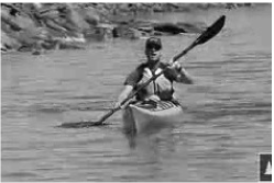
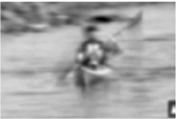
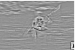
$L_{t,norm}$	$L_{tt,norm}$	$\det{\cal H}_{(x,y),norm}L$

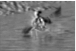
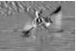
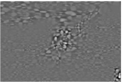
$\partial_{t}(\nabla_{(x,y),norm}^{2}L)$	$\partial_{tt}(\nabla_{(x,y),norm}^{2}L)$	$-\sqrt{{\cal Q}_{t}(\nabla_{(x,y),norm}^{2}L)}$

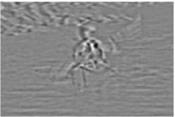
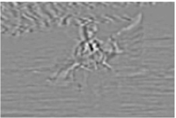
$\det{\cal H}_{(x,y,t),norm}L$	${\cal G}_{(x,y,t),norm}L$	$-\sqrt[3]{{\cal Q}_{t}(\det{\cal H}_{(x,y),norm}L)}$

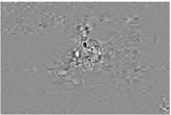
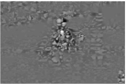
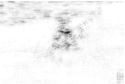
$-\sqrt{{\cal Q}_{1,(x,y,t),norm}L}$	$-\sqrt{{\cal Q}_{2,(x,y,t),norm}L}$	$-\sqrt{{\cal Q}_{3,(x,y,t),norm}L}$

Figure 7: Spatio-temporal features computed from a video sequence in the UCF-101 dataset (Kayaking_g01_c01.avi, cropped) at spatial scale $\sigma_{x}=2~{}\mbox{pixels}$ and temporal scale $\sigma_{t}=0.2~{}\mbox{seconds}$ using the proposed separable spatio-temporal receptive field model with Gaussian filtering over the spatial domain and here a cascade of 7 recursive filters over the temporal domain with a logarithmic distribution of the intermediate scale levels for $c=\sqrt{2}$ and with $L_{p}$-normalization of both the spatial and temporal derivative operators. Each figure shows a snapshot around frames 90-97 for the spatial or spatio-temporal differential expression shown above the figure with in some cases additional monotone stretching of the magnitude values to simplify visual interpretation. (Image size: $258\times 172$ pixels of original $320\times 240$ pixels and 226 frames at 25 frames per second.)

8.5 Scale normalized spatio-temporal derivative expressions

For regular partial derivatives, normalization with respect to spatial and temporal scales of a spatio-temporal scale-space derivative of order $m=(m_{1},m_{2})$ over space and order $n$ over time is performed according to

$$L_{x_{1}^{m_{1}}x_{2}^{m_{2}}t^{n},norm}=s^{(m_{1}+m_{2})/2}\,\alpha_{n}(\tau)\,L_{x_{1}^{m_{1}}x_{2}^{m_{2}}t^{n}}$$ (111)

Scale normalization of the spatio-temporal differential expressions in section 8.4 is then performed by replacing each spatio-temporal partial derivate by its corresponding scale-normalized expression (see Lin15-arXiv-spattemp for additional details).

For example, for the three quasi quadrature entities in equations (LABEL:eq-Q1-not-scalenorm-ders), (LABEL:eq-Q2-not-scalenorm-ders) and (LABEL:eq-Q3-not-scalenorm-ders), their corresponding scale-normalized expressions are of the form:

$$\begin{split}&{\cal Q}_{1,(x,y,t),norm}L\end{split}$$

$$\begin{split}&=s\,(L_{x}^{2}+L_{y}^{2})+\alpha_{1}^{2}(\tau)\,\varkappa^{2}L_{t}^{2}+\end{split}$$

$$\begin{split}&\phantom{=}\,+C\left(s^{2}(L_{xx}^{2}+2L_{xy}^{2}+L_{yy}^{2})\right.\end{split}$$

$$\begin{split}&\phantom{=\,+C\left(\right.}\left.+s\,\alpha_{1}^{2}(\tau)\,\varkappa^{2}(L_{xt}^{2}+L_{yt}^{2})+\alpha_{2}^{2}(\tau)\,\varkappa^{4}L_{tt}^{2}\right),\end{split}$$ (112)

$$\begin{split}&{\cal Q}_{2,(x,y,t),norm}L\end{split}$$

$$\begin{split}&={\cal Q}_{t,norm}L\times{\cal Q}_{(x,y),norm}L\end{split}$$

$$\begin{split}&=\left(\alpha_{1}^{2}(\tau)\,L_{t}^{2}+C\,\alpha_{2}^{2}(\tau)\,L_{tt}^{2}\right)\times\end{split}$$

$$\begin{split}&\phantom{=\left(\right.}\left(s\,(L_{x}^{2}+L_{y}^{2})+C\,s^{2}\left(L_{xx}^{2}+2L_{xy}^{2}+L_{yy}^{2}\right)\right),\end{split}$$ (113)

$$\begin{split}&{\cal Q}_{3,(x,y,t),norm}L\end{split}$$

$$\begin{split}&={\cal Q}_{(x,y),norm}L_{t}+C\,{\cal Q}_{(x,y),norm}L_{tt}\end{split}$$

$$\begin{split}&=\alpha_{1}^{2}(\tau)\left(s\,(L_{xt}^{2}+L_{yt}^{2})+C\,s^{2}\left(L_{xxt}^{2}+2L_{xyt}^{2}+L_{yyt}^{2}\right)\right)\end{split}$$

$$\begin{split}&\phantom{=}\,+C\,\alpha_{2}^{2}(\tau)\left(s\,(L_{xtt}^{2}+L_{ytt}^{2})\right.\end{split}$$

$$\begin{split}&\phantom{=+C\,\alpha_{2}^{2}(\tau)\left(\right.}\left.+Cs^{2}(L_{xxtt}^{2}+2L_{xytt}^{2}+L_{yytt}^{2})\right).\end{split}$$ (114)

8.6 Experimental results

Figure 7 shows the result of computing the above differential expressions for a video sequence of a paddler in a kayak.

Comparing the spatio-temporal scale-space representation $L$ in the top middle figure to the original video $f$ in the top left, we can first note that a substantial amount of fine scale spatio-temporal textures, e.g. waves of the water surface, is suppressed by the spatio-temporal smoothing operation. The illustrations of the spatio-temporal scale-space representation $L$ in the top middle figure and its first- and second-order temporal derivatives $L_{t,norm}$ and $L_{tt,norm}$ in the left and middle figures in the second row do also show the spatio-temporal traces that are left by a moving object; see in particular the image structures below the raised paddle that respond to spatial points in the image domain where the paddle has been in the past.

The slight jagginess in the bright response that can be seen below the paddle in the response to the second-order temporal derivative $L_{tt,norm}$ is a temporal sampling artefact caused by sparse temporal sampling in the original video. With 25 frames per second there are 40 ms between adjacent frames, during which there may happen a lot in the spatial image domain for rapidly moving objects. This situation can be compared to mammalian vision where many receptive fields operate continuously over time scales in the range 20-100 ms. With 40 ms between adjacent frames it is not possible to simulate such continuous receptive fields smoothly over time, since such a frame rate corresponds to either zero, one or at best two images within the effective time span of the receptive field. To simulate rapid continuous time receptive fields more accurately in a digital implementation, one should therefore preferably aim at acquiring the input video with a higher temporal frame rate. Such higher frame rates are indeed now becoming available, even in consumer cameras. Despite this limitation in the input data, we can observe that the proposed model is able to compute geometrically meaningful spatio-temporal image features from the raw video.

The illustrations of $\partial_{t}(\nabla_{(x,y),norm}^{2}L)$ and $\partial_{tt}(\nabla_{(x,y),norm}^{2}L)$ in the left and middle of the third row show the responses of our idealized model of non-lagged and lagged LGN cells complemented by a quasi-quadrature energy measure of these responses in the right column. These entities correspond to applying a spatial Laplacian operator to the first- and second-order temporal derivatives in the second row and it can be seen how this operation enhances spatial variations. These spatio-temporal entities can also be compared to the purely spatial interest operators, the Laplacian $\nabla_{(x,y),norm}^{2}L$ and the determinant of the Hessian $\det{\cal H}_{(x,y),norm}L$ in the first and second rows of the third column. Note how the genuinely spatio-temporal recursive fields enhance spatio-temporal structures compared to purely spatial operators and how static structures, such as the label in the lower right corner, disappear altogether by genuine spatio-temporal operators. The fourth row shows how three other genuine spatio-temporal operators, the spatio-temporal Hessian $\partial_{t}(\nabla_{(x,y),norm}^{2}L)$, the rescaled Gaussian curvature ${\cal G}_{(x,y,t),norm}L$ and the quasi quadrature measure ${\cal Q}_{t}(\det{\cal H}_{(x,y),norm}L)$, also respond to points where there are simultaneously both strong spatial and strong temporal variations.

The bottom row shows three idealized models defined to mimic qualitatively known properties of complex cells and expressed in terms of quasi quadrature measures of spatio-temporal scale-space derivatives. For the first quasi quadrature entity ${\cal Q}_{1,(x,y,t),norm}L$ to respond, in which time is treated in a largely qualitatively similar manner as space, it is sufficient if there are strong variations over either space or time. It can be seen that this measure is therefore not highly selective. For the second and the third entities ${\cal Q}_{2,(x,y,t),norm}L$ and ${\cal Q}_{3,(x,y,t),norm}L$, it is necessary that there are simultaneous variations over both space and time, and it can be seen how these entities are as a consequence more selective. For the third entity ${\cal Q}_{3,(x,y,t),norm}L$, simultaneous selectivity over both space and time is additionally enforced on each primitive linear receptive field that is then combined into the non-linear quasi quadrature measure. We can see how this quasi quadrature entity also responds stronger to the moving paddle than the two other quasi quadrature measures.

8.7 Geometric covariance and invariance properties

Rotations in image space.

The spatial differential expressions $|\nabla_{(x,y)}L|$, $\nabla_{(x,y)}^{2}L$, $\det{\cal H}_{(x,y)}$, $\tilde{\kappa}(L)$ and ${\cal Q}_{(x,y)}L$ are all invariant under rotations in the image domain and so are the spatio-temporal derivative expressions $\partial_{t}(\nabla_{(x,y)}^{2}L)$, $\partial_{tt}(\nabla_{(x,y)}^{2}L)$, ${\cal Q}_{t}(\nabla_{(x,y)}^{2}L)$, $\partial_{t}(\det{\cal H}_{(x,y)}L)$, $\partial_{tt}(\det{\cal H}_{(x,y)}L)$, ${\cal Q}_{t}(\det{\cal H}_{(x,y)}L)$, $\det{\cal H}_{(x,y,t)}L$, ${\cal G}_{(x,y,t)}L$, $\nabla_{(x,y,t)}^{2}L$, ${\cal Q}_{1,(x,y,t)}L$, ${\cal Q}_{2,(x,y,t)}L$ and ${\cal Q}_{3,(x,y,t)}L$ as well as their corresponding scale-normalized expressions.

Uniform rescaling of the spatial domain.

Under a uniform scaling transformation of image space, the spatial differential invariants $|\nabla_{(x,y)}L|$, $\nabla_{(x,y)}^{2}L$, $\det{\cal H}_{(x,y)}$ and $\tilde{\kappa}(L)$ are covariant under spatial scaling transformations in the sense that their magnitude values are multiplied by a power of the scaling factor, and so are their corresponding scale-normalized expressions. Also the spatio-temporal differential invariants $\partial_{t}(\nabla_{(x,y)}^{2}L)$, $\partial_{tt}(\nabla_{(x,y)}^{2}L)$, $\partial_{t}(\det{\cal H}_{(x,y)}L)$, $\partial_{tt}(\det{\cal H}_{(x,y)}L)$, $\det{\cal H}_{(x,y,t)}L$ and ${\cal G}_{(x,y,t)}L$ and their corresponding scale-normalized expressions are covariant under spatial scaling transformations in the sense that their magnitude values are multiplied by a power of the scaling factor under such spatial scaling transformations.

The quasi quadrature entity ${\cal Q}_{(x,y),norm}L$ is however not covariant under spatial scaling transformations and not the spatio-temporal differential invariants ${\cal Q}_{t,norm}(\nabla_{(x,y)}^{2}L)$,
${\cal Q}_{t,norm}(\det{\cal H}_{(x,y)}L)$, ${\cal Q}_{1,(x,y,t),norm}L$, ${\cal Q}_{2,(x,y,t),norm}L$ and ${\cal Q}_{3,(x,y,t),norm}L$ either. Due to the form of ${\cal Q}_{(x,y),norm}L$, ${\cal Q}_{t,norm}(\nabla_{(x,y)}^{2}L)$, ${\cal Q}_{t,norm}(\det{\cal H}_{(x,y)}L)$, ${\cal Q}_{2,(x,y,t),norm}L$ and ${\cal Q}_{3,(x,y,t),norm}L$ as being composed of sums of scale-normalized derivative expressions for $\gamma=1$, these derivative expressions can, however, anyway be made scale invariant when combined with a spatial scale selection mechanism.

Uniform rescaling of the temporal domain independent of the spatial domain.

Under an independent rescaling of the temporal dimension while keeping the spatial dimension fixed, the partial derivatives $L_{x_{1}^{m_{1}}x_{2}^{m_{1}}t^{n}}(x_{1},x_{2},t;\;s,\tau)$ are covariant under such temporal rescaling transformations, and so are the directional derivatives $L_{\varphi^{m_{1}}\bot\varphi^{m_{2}}t^{n}}$ for image velocity $v=0$. For non-zero image velocities, the image velocity parameters of the receptive field would on the other hand need to be adapted to the local motion direction of the objects/spatio-temporal events of interest to enable matching between corresponding spatio-temporal directional derivative operators.

Under an independent rescaling of the temporal dimension while keeping the spatial dimension fixed, also the spatio-temporal differential invariants $\partial_{t}(\nabla_{(x,y)}^{2}L)$, $\partial_{tt}(\nabla_{(x,y)}^{2}L)$, $\partial_{t}(\det{\cal H}_{(x,y)}L)$, $\partial_{tt}(\det{\cal H}_{(x,y)}L)$, $\det{\cal H}_{(x,y,t)}L$ and ${\cal G}_{(x,y,t)}L$ are covariant under independent rescaling of the temporal vs. spatial dimensions. The same applies to their corresponding scale-normalized expressions.

The spatio-temporal differential invariants ${\cal Q}_{t,norm}(\nabla_{(x,y)}^{2}L)$, ${\cal Q}_{t,norm}(\det{\cal H}_{(x,y)}L)$, ${\cal Q}_{1,(x,y,t),norm}L$, ${\cal Q}_{2,(x,y,t),norm}L$ and ${\cal Q}_{3,(x,y,t),norm}L$ are however not covariant under independent rescaling of the temporal vs. spatial dimensions and would therefore need a temporal scale selection mechanism to enable temporal scale invariance.

$-\sqrt{{\cal Q}_{1,(x,y,t),norm}L}$	$-\sqrt{{\cal Q}_{2,(x,y,t),norm}L}$	$-\sqrt{{\cal Q}_{3,(x,y,t),norm}L}$

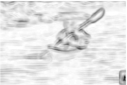
Figure 8: Illustration of the influence of temporal illumination or exposure compensation mechanisms on spatio-temporal receptive field responses, computed from the video sequence Kayaking_g01_c01.avi (cropped) in the UCF-101 dataset. Each figure shows a snapshot at frame 8 for the quasi quadrature entity shown above the figure with additional monotone stretching of the magnitude values to simplify visual interpretation. Note how the time varying illumination or exposure compensation leads to a strong overall response in the first quasi quadrature entity ${\cal Q}_{1,(x,y,t),norm}L$ caused by strong responses in the purely temporal derivatives $L_{t}$ and $L_{tt}$, whereas the responses of second and the third quasi quadrature entities ${\cal Q}_{2,(x,y,t),norm}L$ and ${\cal Q}_{3,(x,y,t),norm}L$ are much less influenced. Indeed, for a logarithmic brightness scale the third quasi quadrature entity ${\cal Q}_{3,(x,y,t),norm}L$ is invariant under such multiplicative illumination or exposure compensation variations.

8.8 Invariance to illumination variations and exposure control mechanisms

Because of all these expressions being composed of spatial, temporal and spatio-temporal derivatives of non-zero order, it follows that all these differential expressions are invariant under additive illumination transformations of the form $L\mapsto L+C$.

This means that if we would take the image values $f$ as representing the logarithm of the incoming energy $f\sim\log I$ or $f\sim\log I^{\gamma}=\gamma\log I$, then all these differential expressions will be invariant under local multiplicative illumination transformations of the form $I\mapsto C\,I$ implying $L\sim\log I+\log C$ or $L\sim\log I^{\gamma}=\gamma(\log I+\log C)$. Thus, these differential expressions will be invariant to local multiplicative variabilities in the external illumination (with locality defined as over the support region of the spatio-temporal receptive field) or multiplicative exposure control parameters such as the aperture of the lens and the integration time or the sensitivity of the sensor.

More formally, let us assume a (i) perspective camera model extended with (ii) a thin circular lens for gathering incoming light from different directions and (iii) a Lambertian illumination model extended with (iv) a spatially varying albedo factor for modelling the light that is reflected from surface patterns in the world. Then, by theoretical results in (Lindeberg (Lin13-BICY, , section 2.3)) a spatio-temporal receptive field response $L_{x^{m_{1}}y^{m_{2}}t^{n}}(\cdot,\cdot;\;s,\tau)$ where ${\cal T}_{s,\tau}$ represents the spatio-temporal smoothing operator can be expressed as

$$\begin{split}&L_{x^{m_{1}}y^{m_{2}}t^{n}}\end{split}$$

$$\begin{split}&=\partial_{x^{m_{1}}y^{m_{2}}t^{n}}\,{\cal T}_{s,\tau}\,\left(\log\rho(x,y,t)+\log i(x,y,t)\vphantom{\log C_{cam}(\tilde{f}(t))}\right.\end{split}$$

$$\begin{split}&\phantom{=\partial_{x^{m_{1}}y^{m_{2}}t^{n}}\,{\cal T}_{s,\tau}\,\left(\right.}\left.+\log C_{cam}(\tilde{f}(t))+V(x,y)\right)\end{split}$$ (115)

where (i) $\rho(x,y,t)$ is a spatially dependent albedo factor, (ii) $i(x,y,t)$ denotes a spatially dependent illumination field, (iii) $C_{cam}(\tilde{f}(t))=\frac{\pi}{4}\frac{d}{f}$ represents possibly time-varying internal camera parameters and (iv) $V(x,y)=-2\log(1+x^{2}+y^{2})$ represents a geometric natural vignetting effect.

From the structure of equation (LABEL:eq-illum-model-spat-rec-field) we can note that for any non-zero order of spatial differentiation $m_{1}+m_{2}>0$, the influence of the internal camera parameters in $C_{cam}(\tilde{f}(t))$ will disappear because of the spatial differentiation with respect to $x_{1}$ or $x_{2}$, and so will the effects of any other multiplicative exposure control mechanism. Furthermore, for any multiplicative illumination variation $i^{\prime}(x,y)=C\,i(x,y)$, where $C$ is a scalar constant, the logarithmic luminosity will be transformed as $\log i^{\prime}(x,y)=\log C+\log i(x,y)$, which implies that the dependency on $C$ will disappear after spatial differentiation. For purely temporal derivative operators, that do not involve any order of spatial differentiation, such as the first- and second-order derivative operators, $L_{t}$ and $L_{tt}$, strong responses may on the other hand be obtained due to illumination compensation mechanisms that vary over time as the results of rapid variations in the illumination. If one wants to design spatio-temporal feature detectors that are robust to illumination variations and to variations in exposure compensation mechanisms caused by these, it is therefore essential to include non-zero orders of spatial differentiation. The use of Laplacian-like filtering in the first stages of visual processing in the retina and the LGN can therefore be interpreted as a highly suitable design to achieve robustness of illumination variations and adaptive variations in the diameter of the pupil caused by these, while still being expressed in terms of rotationally symmetric linear receptive fields over the spatial domain.

If we extend this model to the simplest form of position- and time-dependent illumination and/or exposure variations as modelled on the form

$$L\mapsto L+Ax+By+Ct$$ (116)

then we can see that the spatio-temporal differential invariants $\partial_{t}(\nabla_{(x,y)}^{2}L)$, $\partial_{tt}(\nabla_{(x,y)}^{2}L)$, ${\cal Q}_{t}(\nabla_{(x,y)}^{2}L)$, $\partial_{t}(\det{\cal H}_{(x,y)}L)$, $\partial_{tt}(\det{\cal H}_{(x,y)}L)$, ${\cal Q}_{t}(\det{\cal H}_{(x,y)}L)$, $\det{\cal H}_{(x,y,t)}L$, ${\cal G}_{(x,y,t)}L$ $\nabla_{(x,y,t)}^{2}L$ and ${\cal Q}_{3,(x,y,t)}L$ are all invariant under such position- and time-dependent illumination and/or exposure variations.

The quasi quadrature entities ${\cal Q}_{1,(x,y,t)}L$ and ${\cal Q}_{2,(x,y,t)}L$ are however not invariant to such position- and time-dependent illumination variations. This property can in particular be noted for the quasi quadrature entity ${\cal Q}_{1,(x,y,t)}L$, for which what seems as initial time-varying exposure compensation mechanisms in the camera lead to large responses in the initial part of the video sequence (see figure 8(left)). Out of the three quasi quadrature entities ${\cal Q}_{1,(x,y,t)}L$, ${\cal Q}_{2,(x,y,t)}L$ and ${\cal Q}_{3,(x,y,t)}L$, the third quasi quadrature entity does therefore possess the best robustness properties to illumination variations (see figure 8(right)).

9 Summary and discussion

We have presented an improved computational model for spatio-temporal receptive fields based on time-causal and time-recursive spatio-temporal scale-space representation defined from a set of first-order integrators or truncated exponential filters coupled in cascade over the temporal domain in combination with a Gaussian scale-space concept over the spatial domain. This model can be efficiently implemented in terms of recursive filters over time and we have shown how the continuous model can be transferred to a discrete implementation while retaining discrete scale-space properties. Specifically, we have analysed how remaining design parameters within the theory, in terms of the number of first-order integrators coupled in cascade and a distribution parameter of a logarithmic distribution, affect the temporal response dynamics in terms of temporal delays.

Compared to other spatial and temporal scale-space representations based on continuous scale parameters, a conceptual difference with the temporal scale-space representation underlying the proposed spatio-temporal receptive fields, is that the temporal scale levels have to be discrete. Thereby, we sacrifice a continuous scale parameter and full scale invariance as resulting from the Gaussian scale-space concepts based on causality or non-enhancement of local extrema (Koenderink Koe84 ; Lindeberg Lin10-JMIV ) or used as a scale-space axiom in certain axiomatic scale-space formulations (Iijima Iij62 ; Florack et al. FloRom92-IVC ; Pauwels et al. PauFidMooGoo95-PAMI ; Weickert et al. WeiIshImi96-ScSp ; Wei98-book ; WeiIshImi99-JMIV ; Duits et al. DuiFelFloPla03-SCSP ; DuiFloGraRom04-JMIV ; Fagerström Fag05-IJCV ; Fag07-ScSp ); see also Witkin Wit83 , Babaud et al. BWBD86-PAMI , Yuille and Poggio YuiPog86-PAMI , Koenderink and van Doorn KoeDoo90-BC ; KoeDoo92-PAMI , Lindeberg Lin90-PAMI ; Lin93-Dis ; Lin94-SI ; Lin96-ScSp ; Lin97-ICSSTCV ; Lin13-ImPhys , Florack et al. FloRomKoeVie92-ECCV ; FloRom92-IVC ; Flo97-book , Alvarez et al. Alv92-TR , Guichard Gui98-TIP , ter Haar Romeny et al. RomFloNie01-SCSP ; Haa94-GDDbook , Felsberg and Sommer FelSom04-JMIV and Tschirsich and Kuijper TscKui15-JMIV for other scale-space approaches closely related to this work, as well as Fleet and Langley FleLan95-PAMI , Freeman and Adelson FreAde91-PAMI , Simoncelli et al. SimFreAdeHee92-IT and Perona per92-ivc for more filter-oriented approaches, Miao and Rao MiaRao07-NeurComp , Duits and Burgeth DuiBur07-ScSp , Cocci et al.  CocBarSar12-JOSA , Barbieri et al. BarCitCocSar14-JMIV and Sharma and Duits ShaDui14-HarmAnal for Lie group approaches for receptive fields and Lindeberg and Friberg LinFri15-PONE ; LinFri15-SSVM for the application of closely related principles for deriving idealized computational models of auditory receptive fields.

When using a logarithmic distribution of the intermediate scale levels, we have however shown that by a limit construction when the number of intermediate temporal scale levels tends to infinity, we can achieve true self-similarity and scale invariance over a discrete set of scaling factors. For a vision system intended to operate in real time using no other explicit storage of visual data from the past than a compact time-recursive buffer of spatio-temporal scale-space at different temporal scales, the loss of a continuous temporal scale parameter may however be less of a practical constraint, since one would anyway have to discretize the temporal scale levels in advance to be able to register the image data to be able to perform any computations at all.

In the special case when all the time constants of the first-order integrators are equal, the resulting temporal smoothing kernels in the continuous model (29) correspond to Laguerre functions (Laguerre polynomials multiplied by a truncated exponential kernel), which have been previously used for modelling the temporal response properties of neurons in the visual system (den Brinker and Roufs BriRou92-BC ) and for computing spatio-temporal image features in computer vision (Rivero-Moreno and Bres RivBre04-ImAnalRec ; Berg et al. BerReyRid14-SensMEMSElOptSyst ). Regarding the corresponding discrete model with all time constants equal, the corresponding discrete temporal smoothing kernels approach Poisson kernels when the number of temporal smoothing steps increases while keeping the variance of the composed kernel fixed (Lindeberg and Fagerström LF96-ECCV ). Such Poisson kernels have also been used for modelling biological vision (Fourtes and Hodgkin FouHod64-JPhys ). Compared to the special case with all time constants equal, a logarithmic distribution of the intermediate temporal scale levels (18) does on the other hand allow for larger flexibility in the trade-off between temporal smoothing and temporal response characteristics, specifically enabling faster temporal responses (shorter temporal delays) and higher computational efficiency when computing multiple temporal or spatio-temporal receptive field responses involving coarser temporal scales.

From the detailed analysis in section 5 and appendix A we can conclude that when the number of first-order integrators that are coupled in cascade increases while keeping the variance of the composed kernel fixed, the time-causal kernels obtained by composing truncated exponential kernels with equal time constants in cascade tend to a limit kernel with skewness and kurtosis measures zero, or equivalently third- and fourth-order cumulants equal to zero, whereas the time-causal kernels obtained by composing truncated exponential kernels having a logarithmic distribution of the intermediate scale levels tends to a limit kernel with non-zero skewness and non-zero kurtosis This property reveals a fundamental difference between the two classes of time-causal scale-space kernels based on either a logarithmic or a uniform distribution of the intermediate temporal scale levels.

In a complementary analysis in appendix B, we have also shown how our time-causal kernels can be related to the temporal kernels in Koenderink’s scale-time model Koe88-BC . By identifying the first- and second-order temporal moments of the two classes of kernels, we have derived closed-form expressions to relate the parameters between the two models, and showed that although the two classes of kernels to a large extent share qualitatively similar properties, the two classes of kernels differ significantly in terms of their third- and fourth-order skewness and kurtosis measures.

The closed-form expressions for Koenderink’s scale-time kernels are analytically simpler than the explicit expressions for our kernels, which will be sums of truncated exponential kernels for all the time constants with the coefficients determined from a partial fraction expansion. In this respect, the derived mapping between the parameters of our and Koenderink’s models can be used e.g. for estimation the time of the temporal maximum of our kernels, which would otherwise have to be determined numerically. Our kernels do on the other hand have a clear computational advantage in that they are truly time-recursive, meaning that the primitive first-order integrators in the model contain sufficient information for updating the model to new states over time, whereas the kernels in Koenderink’s scale-time model appear to require a complete memory of the past, since they do not have any known time-recursive formulation.

Regarding the purely temporal scale-space concept used in our spatio-temporal model, we have notably replaced the assumption of a semi-group structure over temporal scales by a weaker Markov property, which however anyway guarantees a necessary cascade property over temporal scales, to ensure gradual simplification of the temporal scale-space representation from any finer to any coarser temporal scale. By this relaxation of the requirement of a semi-group over temporal scales, we have specifically been able to define a temporal scale-space concept with much better temporal dynamics than the time-causal semi-groups derived by Fagerström Fag05-IJCV and Lindeberg Lin10-JMIV . Since this new time-causal temporal scale-space concept with a logarithmic distribution of the intermediate temporal scale levels would not be found if one would start from the assumption about a semi-group over temporal scales as a necessary requirement, we propose that that in the area of scale-space axiomatics the assumption of a semi-group over temporal scales should not be regarded as a necessary requirement for a time-causal temporal scale-space representation.

Recently, and during the development of this article, Mahmoudi Mah15-soton-preprint has presented a very closely related while more neurophysiologically motivated model for visual receptive fields, based on an electrical circuit model with spatial smoothing determined by local spatial connections over a spatial grid and temporal smoothing by first-order temporal integration. The spatial component in that model is very closely related to our earlier discrete scale-space models over spatial and spatio-temporal grids (Lindeberg Lin90-PAMI ; Lin97-ICSSTCV ; Lin02-ECCV ) as can be modelled by Z-transforms of the discrete convolution kernels and an algebra of spatial or spatio-temporal covariance matrices to model the transformation properties of the receptive fields under locally linearized geometric image transformations. The temporal component in that model is in turn similar to our temporal smoothing model by first-order integrators coupled in cascade as initially proposed in (Lindeberg Lin90-PAMI ; Lindeberg and Fagerström LF96-ECCV ), suggested as one of three models for temporal smoothing in spatio-temporal visual receptive fields in (Lindeberg Lin13-BICY ; Lin13-ImPhys ) and then refined and further developed in (Lindeberg Lin15-SSVM ; Lin15-arXiv-spattemp ) and this article. Our model can also be implemented by electric circuits, by combining the temporal electric model in figure 2 with the spatial discretization in section 6.3 or more general connectivities between adjacent layers to implement velocity-adapted receptive fields as can then be described by their resulting spatio-temporal covariance matrices. Mahmoudi compares such electrically modelled receptive fields to results of neurophysiological recordings in the LGN and the primary visual cortex in a similar way as we compared our theoretically derived receptive fields to biological receptive fields in (Lindeberg Lin97-ICSSTCV ; Lin10-JMIV ; Lin13-BICY ; Lin15-SSVM ) and in this article.

Mahmoudi shows that the resulting transfer function in the layered electric circuit model approaches a Gaussian when the number of layers tends to infinity. This result agrees with our earlier results that the discrete scale-space kernels over a discrete spatial grid approach the continuous Gaussian when the spatial scale increment tends to zero while the spatial scale level is held constant Lin90-PAMI and that the temporal smoothing function corresponding to a set of first-order integrators with equal time constants coupled in cascade tend to the Poisson kernel (which in turn approaches the Gaussian kernel) when the temporal scale increment tends to zero while the temporal scale level is held constant LF96-ECCV .

In his article, Mahmoudi Mah15-soton-preprint makes a distinction between our scale-space approach, which is motivated by the mathematical structure of the environment in combination with a set of assumptions about the internal structure of a vision system to guarantee internal consistency between image representations at different spatial and temporal scales, and his model motivated by assumptions about neurophysiology. One way to reconcile these views is by following the evolutionary arguments proposed in (Lindeberg Lin13-BICY ; Lin13-PONE ). If there is a strong evolutionary pressure on a living organism that uses vision as a key source of information about its environment (as there should be for many higher mammals), then in the competition between two species or two individuals from the same species, there should be a strong evolutionary advantage for an organism that as much as possible adapts the structure of its vision system to be consistent with the structural and transformation properties of its environment. Hence, there could be an evolutionary pressure for the vision system of such an organism to develop similar tupes of receptive fields as can be derived by an idealized mathematical theory, and specifically develop neurophysiological wetware that permits the computation of sufficiently good approximations to idealized receptive fields as derived from mathematical and physical principles. From such a viewpoint, it is highly interesting to see that the neurophysiological cell recordings in the LGN and the primary visual cortex presented by DeAngelis et al. DeAngOhzFre95-TINS ; deAngAnz04-VisNeuroSci are in very good qualitative agreement with the predictions generated by our mathematically and physically motivated normative theory (see figure 3 and figure 4).

Given the derived time-causal and time-recursive formulation of our basic linear spatio-temporal receptive fields, we have described how this theory can be used for computing different types of both linear and non-linear scale-normalized spatio-temporal features. Specifically, we have emphasized how scale normalization by $L_{p}$-normalization leads to fundamentally different results compared to more traditional variance-based normalization. By the formulation of the corresponding scale normalization factors for discrete temporal scale space, we have also shown how they permit the formulation of an operational criterion to estimate how many intermediate temporal scale levels are needed to approximate true scale invariance up to a given tolerance.

Finally, we have shown how different types of spatio-temporal features can defined in terms of spatio-temporal differential invariants built from spatio-temporal receptive field responses, including their transformation properties under natural image transformations, with emphasis on independent scaling transformations over space vs. time, rotational invariance over the spatial domain and illumination and exposure control variations. We propose that the presented theory can be used for computing features for generic purposes in computer vision and for computational modelling of biological vision for image data over a time-causal spatio-temporal domain, in an analogous way as the Gaussian scale-space concept constitutes a canonical model for processing image data over a purely spatial domain.

Appendix A Frequency analysis of the time-causal kernels

In this appendix, we will perform an in-depth analysis of the proposed time-causal scale-space kernels with regard to their frequency properties and moment descriptors derived via the Fourier transform, both for the case of a logarithmic distribution of the intermediate temporal scale levels and a uniform distribution of the intermediate temporal scale levels. Specifically, the results to be derived will provide a way to characterize properties of the limit kernel when the number of temporal scale levels $K$ tends to infinity.

A.1 Logarithmic distribution of the intermediate scale levels

In section 5, we gave the following explicit expressions for the Fourier transform of the time-causal kernels based on a logarithmic distribution of the intermediate scale levels

$$\hat{h}_{exp}(\omega;\;\tau,c,K)=\frac{1}{1+i\,c^{1-K}\sqrt{\tau}\,\omega}\prod_{k=2}^{K}\frac{1}{1+i\,c^{k-K-1}\sqrt{c^{2}-1}\sqrt{\tau}\,\omega}$$ (117)

for which the magnitude and the phase are given by

$$\begin{split}&|\hat{h}_{exp}(\omega;\;\tau,c,K)|\end{split}$$

$$\begin{split}&=\frac{1}{\sqrt{1+c^{2(1-K)}\tau\,\omega^{2}}}\prod_{k=2}^{K}\frac{1}{\sqrt{1+c^{2(k-K-1)}(c^{2}-1)\tau\,\omega^{2}}},\end{split}$$ (118)

$$\begin{split}&\arg\hat{h}_{exp}(\omega;\;\tau,c,K)\end{split}$$

$$\begin{split}&=\arctan\left(c^{1-K}\sqrt{\tau}\,\omega\right)+\sum_{k=2}^{K}\arctan\left(c^{k-K-1}\sqrt{c^{2}-1}\sqrt{\tau}\,\omega\right).\end{split}$$

Let us rewrite the magnitude of the Fourier transform on exponential form

$$|\hat{h}_{exp}(\omega;\;\tau,c,K)|=e^{\log|\hat{h}_{exp}(\omega;\;\tau,c,K)|}\\ =e^{-\frac{1}{2}\log(1+c^{2(1-K)}\tau\,\omega^{2})-\frac{1}{2}\sum_{k=2}^{K}\log(1+c^{2(k-K-1)}(c^{2}-1)\tau\,\omega^{2})}$$ (120)

and compute the Taylor expansion of

$$\log|\hat{h}_{exp}(\omega;\;\tau,c,K)|=C_{2}\omega^{2}+C_{4}\omega^{4}+{\cal O}(\omega^{6})$$ (121)

where

$$\begin{split}C_{2}&=-\frac{\tau}{2},\end{split}$$ (122)

$$\begin{split}C_{4}&=-\frac{\tau^{2}\left(-2c^{4-4K}-c^{2}+1\right)}{4\left(c^{2}+1\right)}\rightarrow\frac{\left(c^{2}-1\right)\tau^{2}}{4\left(c^{2}+1\right)},\end{split}$$ (123)

and the rightmost expression for $C_{4}$ shows the limit value when the number $K$ of first-order integrators coupled in cascade tends to infinity.

Let us next compute the Taylor expansion of

$$\arg\hat{h}_{exp}(\omega;\;\tau,c,K)=C_{1}\omega+C_{3}\omega^{3}+{\cal O}(\omega^{5})$$ (124)

where the coefficients are given by

$$\begin{split}C_{1}&=\frac{\sqrt{\tau}c^{-K}\left(-c^{2}+\sqrt{c^{2}-1}c-\sqrt{c^{2}-1}c^{K}+c\right)}{c-1}\end{split}$$

$$\begin{split}\rightarrow-\frac{\sqrt{\left(c^{2}-1\right)}\,\sqrt{\tau}}{c-1},\end{split}$$ (125)

$$\begin{split}C_{3}&=\frac{\sqrt{c^{2}-1}\tau^{3/2}}{3\left(c^{2}+c+1\right)}\left(\left(c^{3K}+c^{3K+1}-c^{4}-c^{3}\right)c^{-3K}\right.\end{split}$$

$$\begin{split}&\phantom{=\frac{\sqrt{c^{2}-1}\tau^{3/2}}{3\left(c^{2}+c+1\right)}\left(\right.}\left.+\left(c^{5}+c^{4}+c^{3}\right)\tau^{3/2}c^{-3K}\right)\end{split}$$

$$\begin{split}&\phantom{=}\rightarrow\frac{(c+1)\sqrt{c^{2}-1}\,\tau^{3/2}}{3\left(c^{2}+c+1\right)},\end{split}$$ (126)

and again the rightmost expressions for $C_{1}$ and $C_{3}$ show the limit values when the number $K$ of scale levels tends to infinity.

Following the definition of cumulants $\kappa_{n}$ defined as the Taylor coefficients of the logarithm of the Fourier transform

$$\log h(\omega)=\sum_{n=0}^{\infty}\kappa_{n}\frac{(-i\omega)^{n}}{n!},$$ (127)

we obtain

$$\begin{split}&\log\hat{h}_{exp}(\omega;\;\tau,c,K)\end{split}$$

$$\begin{split}&=-C_{1}(-i\omega)-C_{2}(-i\omega)^{2}+C_{3}(-i\omega)^{3}+C_{4}(-i\omega)^{4}+{\cal O}(i\omega^{5})\end{split}$$

$$\begin{split}&=\kappa_{0}+\frac{\kappa_{1}}{1!}(-i\omega)+\frac{\kappa_{2}}{2!}(-i\omega^{2})+\frac{\kappa_{3}}{3!}(-i\omega)^{3}+\frac{\kappa_{4}}{4!}(-i\omega)^{4}+{\cal O}(i\omega^{5})\end{split}$$ (128)

and can read the cumulants of the underlying temporal scale-space kernel as $\kappa_{0}=0$, $\kappa_{1}=-C_{1}$, $\kappa_{2}=-2C_{2}$, $\kappa_{3}=6C_{3}$ and $\kappa_{4}=24C_{4}$. Specifically, the first-order moment $M_{1}$ and the higher-order central moments $M_{2}$, $M_{3}$ and $M_{4}$ are related to the cumulants according to

$$\begin{split}M_{1}&=\kappa_{1}=-C_{1}\rightarrow\frac{\sqrt{\left(c^{2}-1\right)}\,\sqrt{\tau}}{c-1},\end{split}$$ (129)

$$\begin{split}M_{2}&=\kappa_{2}=-2C_{2}=\tau,\end{split}$$ (130)

$$\begin{split}M_{3}&=\kappa_{3}=6C_{3}\rightarrow\frac{2(c+1)\sqrt{c^{2}-1}\,\tau^{3/2}}{\left(c^{2}+c+1\right)},\end{split}$$ (131)

$$\begin{split}M_{4}&=\kappa_{4}+3\kappa_{2}^{2}=24C_{4}+12C_{2}^{2}\rightarrow\frac{3\left(3c^{2}-1\right)\tau^{2}}{c^{2}+1}.\end{split}$$ (132)

Thus, the skewness $\gamma_{1}$ and the kurtosis $\gamma_{2}$ measures of the corresponding temporal scale-space kernels are given by

$$\begin{split}\gamma_{1}&=\frac{\kappa_{3}}{\kappa_{2}^{3/2}}=\frac{M_{3}}{M_{2}^{3/2}}=\frac{3C_{3}}{\sqrt{2}(-C_{2})^{3/2}}\rightarrow\frac{2(c+1)\sqrt{c^{2}-1}}{\left(c^{2}+c+1\right)},\end{split}$$ (133)

$$\begin{split}\gamma_{2}&=\frac{\kappa_{4}}{\kappa_{2}^{2}}=\frac{M_{4}}{M_{2}^{2}}-3=6\,\frac{C_{4}}{C_{2}^{2}}\rightarrow\frac{6\left(c^{2}-1\right)}{c^{2}+1}.\end{split}$$ (134)

Figure 9 shows graphs these skewness and kurtosis measures as function of the distribution parameter $c$ for the limit case when the number of scale levels $K$ tends to infinity. As can be seen, both the skewness and the kurtosis measures of the temporal scale-space kernels increase with increasing values of the distribution parameter $c$.

skewness $\gamma_{1}(c)$

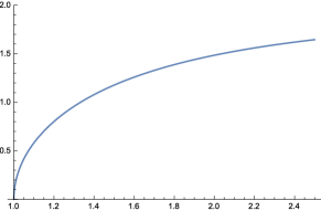
kurtosis $\gamma_{2}(c)$

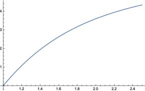
Figure 9: Graphs of the skewness measure $\gamma_{1}$ (133) and the kurtosis measure $\gamma_{2}$ (134) as function of the distribution parameter $c$ for the time-causal scale-space kernels corresponding to limit case of $K$ truncated exponential kernels having a logarithmic distribution of the intermediate scale levels coupled in cascade in the limit case when the number of scale levels $K$ tends to infinity.

A.2 Uniform distribution of the intermediate scale levels

When using a uniform distribution of the intermediate scale levels (16), the time constants of the individual first-order integrators are given by (17) and the explicit expression for the Fourier transform (11) is

$$\hat{h}_{exp}(\omega;\;\tau,K)=\frac{1}{\left(1+i\,\sqrt{\frac{\tau}{K}}\,\omega\right)^{K}}.$$ (135)

Specifically, the magnitude and the phase of the Fourier transform are given by

$$\begin{split}|\hat{h}_{exp}(\omega;\;\tau,K)|&=\frac{1}{\left(1+\frac{\tau}{K}\,\omega^{2}\right)^{K/2}},\end{split}$$ (136)

$$\begin{split}\arg\hat{h}_{exp}(\omega;\;\tau,K)&=-K\arctan\left(\sqrt{\frac{\tau}{K}}\,\omega\right).\end{split}$$ (137)

Let us rewrite the magnitude of the Fourier transform on exponential form

$$\begin{split}|\hat{h}_{exp}(\omega;\;\tau,K)|&=e^{\log|\hat{h}_{exp}(\omega;\;\tau,K)|}=e^{-\frac{K}{2}\log(1+\frac{\tau}{K}\,\omega^{2})}\end{split}$$

and compute the Taylor expansion of

$$\log|\hat{h}_{exp}(\omega;\;\tau,K)|=C_{2}\omega^{2}+C_{4}\omega^{4}+{\cal O}(\omega^{6})$$ (139)

where

$$\begin{split}C_{2}&=-\frac{\tau}{2},\end{split}$$ (140)

$$\begin{split}C_{4}&=\frac{\tau^{2}}{4K}.\end{split}$$ (141)

Next, let us compute the Taylor expansion of

$$\arg\hat{h}_{exp}(\omega;\;\tau,K)=C_{1}\omega+C_{3}\omega^{3}+{\cal O}(\omega^{5})$$ (142)

where the coefficients are given by

$$\begin{split}C_{1}&=-\sqrt{K\tau},\end{split}$$ (143)

$$\begin{split}C_{3}&=\frac{\tau^{3/2}}{3\sqrt{K}}.\end{split}$$ (144)

Following the definition of cumulants $\kappa_{n}$ according to (127), we can in an analogous way to (LABEL:eq-def-cum-from-series-exp-FT) in previous section read $\kappa_{0}=0$, $\kappa_{1}=-C_{1}$, $\kappa_{2}=-2C_{2}$, $\kappa_{3}=6C_{3}$ and $\kappa_{4}=24C_{4}$, and relate the first-order moment $M_{1}$ and the higher-order central moments $M_{2}$, $M_{3}$ and $M_{4}$ to the cumulants according to

$$\begin{split}M_{1}&=\kappa_{1}=-C_{1}=\sqrt{K\tau},\end{split}$$ (145)

$$\begin{split}M_{2}&=\kappa_{2}=-2C_{2}=\tau,\end{split}$$ (146)

$$\begin{split}M_{3}&=\kappa_{3}=6C_{3}=\frac{2\tau^{3/2}}{\sqrt{K}},\end{split}$$ (147)

$$\begin{split}M_{4}&=\kappa_{4}+3\kappa_{2}^{2}=24C_{4}+12C_{2}^{2}=3\tau^{2}+\frac{6\tau^{2}}{K}.\end{split}$$ (148)

Thus, the skewness $\gamma_{1}$ and the kurtosis $\gamma_{2}$ of the corresponding temporal scale-space kernels are given by

$$\begin{split}\gamma_{1}&=\frac{\kappa_{3}}{\kappa_{2}^{3/2}}=\frac{M_{3}}{M_{2}^{3/2}}=\frac{2}{\sqrt{K}},\end{split}$$ (149)

$$\begin{split}\gamma_{2}&=\frac{\kappa_{4}}{\kappa_{2}^{2}}=\frac{M_{4}}{M_{2}^{2}}-3=\frac{6}{K}.\end{split}$$ (150)

From these expressions we can note that when the number $K$ of first-order integrators that are coupled in cascade increases, these skewness and kurtosis measures tend to zero for the temporal scale-space kernels having a uniform distribution of the intermediate temporal scale levels. The corresponding skewness and kurtosis measures (133) and (134) for the kernels having a logarithmic distribution of the intermediate temporal scale levels do on the other hand remain strictly positive. These properties reveal a fundamental difference between the two classes of time-causal kernels obtained by distributing the intermediate scale levels of first-order integrators coupled in cascade according to a logarithmic vs. a uniform distribution.

Appendix B Comparison with Koenderink’s scale-time model

In his scale-time model, Koenderink Koe88-BC proposed to perform a logarithmic mapping of the past via a time delay $\delta$ and then applying Gaussian smoothing on the transformed domain, leading to a time-causal kernel of the form, here largely following the notation in Florack (Flo97-book, , result 4.6, page 116)

$$h_{log}(t;\;\sigma,\delta,a)=\frac{1}{\sqrt{2\pi}\sigma(\delta-a)}e^{-\frac{\log^{2}\left(\frac{t-a}{\delta-a}\right)}{2\sigma^{2}}}$$ (151)

with $a$ denoting the present moment, $\delta$ denoting the time delay and $\sigma$ is a dimensionless temporal scale parameter relative to the logarithmic time axis. For simplicity, we will henceforth assume $a=0$ leading to kernels of the form

$$h_{log}(t;\;\sigma,\delta)=\frac{1}{\sqrt{2\pi}\sigma\,\delta}e^{-\frac{\log^{2}\left(\frac{t}{\delta}\right)}{2\sigma^{2}}}$$ (152)

and with convolution reversal of the time axis such that causality implies $h_{log}(t;\;\sigma,\delta)=0$ for $t<0$. By integrating this kernel symbolically in Mathematica, we find

$$\int_{t=-\infty}^{\infty}h_{log}(t;\;\sigma,\delta)\,dt=e^{\frac{\sigma^{2}}{2}}$$ (153)

implying that the corresponding time-causal kernel normalized to unit $L_{1}$-norm should be

$$h_{Koe}(t;\;\sigma,\delta)=\frac{1}{\sqrt{2\pi}\sigma\,\delta}e^{-\frac{\log^{2}\left(\frac{t}{\delta}\right)}{2\sigma^{2}}-\frac{\sigma^{2}}{2}}.$$ (154)

The temporal mean of this kernel is

$$M_{1}=\bar{t}=\int_{t=-\infty}^{\infty}t\,h_{Koe}(t;\;\sigma,\delta)\,dt=\delta\,e^{\frac{3\sigma^{2}}{2}}$$ (155)

and the higher-order central moments

$$\begin{split}M_{2}&=\int_{t=-\infty}^{\infty}(t-\bar{t})^{2}\,h_{Koe}(t;\;\sigma,\delta)\,dt\end{split}$$

$$\begin{split}&=\delta^{2}e^{3\sigma^{2}}\left(e^{\sigma^{2}}-1\right),\end{split}$$ (156)

$$\begin{split}M_{3}&=\int_{t=-\infty}^{\infty}(t-\bar{t})^{3}\,h_{Koe}(t;\;\sigma,\delta)\,dt\end{split}$$

$$\begin{split}&=\delta^{3}e^{\frac{9\sigma^{2}}{2}}\left(e^{\sigma^{2}}-1\right)^{2}\left(e^{\sigma^{2}}+2\right),\end{split}$$ (157)

$$\begin{split}M_{4}&=\int_{t=-\infty}^{\infty}(t-\bar{t})^{4}\,h_{Koe}(t;\;\sigma,\delta)\,dt\end{split}$$ (158)

$$\begin{split}&=\delta^{4}e^{6\sigma^{2}}\left(e^{\sigma^{2}}-1\right)^{2}\left(3e^{2\sigma^{2}}+2e^{3\sigma^{2}}+e^{4\sigma^{2}}-3\right).\end{split}$$ (159)

skewness $\gamma_{1}(\sigma)$

kurtosis $\gamma_{2}(\sigma)$

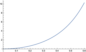
Figure 10: Graphs of the skewness measure $\gamma_{1}$ (160) and the kurtosis measure $\gamma_{2}$ (161) as function of the dimensionless temporal scale parameter $\sigma$ relative to the logarithmic transformation of the past for the time-causal kernels in Koenderink’s scale-time model.

Thus, the skewness $\gamma_{1}$ and the kurtosis $\gamma_{2}$ of the temporal kernels in Koenderink’s scale-time model are given by (see figure 10 for graphs)

$$\begin{split}\gamma_{1}=\frac{M_{3}}{M_{2}^{3/2}}=\sqrt{e^{\sigma^{2}}-1}\left(e^{\sigma^{2}}+2\right),\end{split}$$ (160)

$$\begin{split}\gamma_{2}=\frac{M_{4}}{M_{2}^{2}}-3=3e^{2\sigma^{2}}+2e^{3\sigma^{2}}+e^{4\sigma^{2}}-6.\end{split}$$ (161)

$h(t;\;K=7,c=\sqrt{2})$	$h_{t}(t;\;K=7,c=\sqrt{2}))$	$h_{tt}(t;\;K=7,c=\sqrt{2}))$
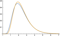
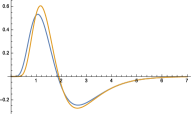
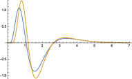
$h(t;\;K=7,c=2^{3/4})$	$h_{t}(t;\;K=7,c=2^{3/4}))$	$h_{tt}(t;\;K=7,c=2^{3/4}))$
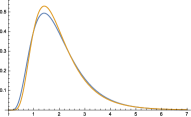
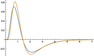
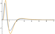
$h(t;\;K=7,c=2)$	$h_{t}(t;\;K=7,c=2))$	$h_{tt}(t;\;K=7,c=2))$

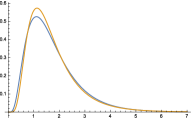
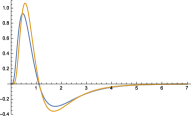
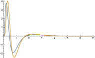
Figure 11: Comparison between the proposed time-causal kernels corresponding to the composition of truncated exponential kernels in cascade (blue curves) for a logarithmic distribution of the intermediate scale levels and the temporal kernels in Koenderink’s scale-time model (brown curves) shown for both the original smoothing kernels and their first- and second-order temporal derivatives. All kernels correspond to temporal scale (variance) $\tau=1$ with the additional parameters determined such that the temporal mean values (the first-order temporal moments) become equal in the limit case when the number of temporal scale levels $K$ tends to infinity (equation (164)). (top row) Logarithmic distribution of the temporal scale levels for $c=\sqrt{2}$ and $K=10$. (middle row) Corresponding results for $c=2^{3/4}$ and $K=10$. (bottom row) Corresponding results for $c=2$ and $K=10$.

If we want to relate these kernels in Koenderink’s scale-time model to our time-causal scale-space kernels, a natural starting point is to require that the total amount of temporal smoothing as measured by the variances $M_{2}$ of the two kernels should be equal. Then, this implies the relation

$$\tau=\delta^{2}e^{3\sigma^{2}}\left(e^{\sigma^{2}}-1\right).$$ (162)

If we additionally relate the kernels by enforcing the temporal delays as measured by the first-order temporal moments to be equal, then we obtain for the limit case when $K\rightarrow\infty$

$${\bar{t}}=\sqrt{\frac{c+1}{c-1}}\sqrt{\tau}=\delta\,e^{\frac{3\sigma^{2}}{2}}.$$ (163)

Solving the system of equations (162) and (163) then gives the following mappings between the parameters in the two temporal scale-space models

$$\left\{\begin{array}[]{l}\tau=\delta^{2}\,e^{3\sigma^{2}}\left(e^{\sigma^{2}}-1\right)\\ c=\frac{e^{\sigma^{2}}}{2-e^{\sigma^{2}}}\end{array}\right.\quad\quad\left\{\begin{array}[]{l}\sigma=\sqrt{\log\left(\frac{2c}{c+1}\right)}\\ \delta=\frac{(c+1)^{2}\sqrt{\tau}}{2\sqrt{2}\sqrt{(c-1)c^{3}}}\end{array}\right.$$ (164)

which hold as long as $c>1$ and $\sigma<\sqrt{\log 2}\approx 0.832$. Specifically, for small values of $\sigma$ a series expansion of the relations to the left gives

$$\left\{\begin{array}[]{l}\tau=\delta^{2}\sigma^{2}\left(1+\frac{7\sigma^{2}}{2}+\frac{37\sigma^{4}}{6}+\frac{175\sigma^{6}}{24}+{\cal O}(\sigma^{8})\right),\\ c=1+2\sigma^{2}+3\sigma^{4}+\frac{13\sigma^{6}}{3}+{\cal O}(\sigma^{8}).\end{array}\right.$$ (165)

If we additionally reparameterize the distribution parameter $c$ such that $c=2^{a}$ for some $a>0$ and perform a series expansion, we obtain

$$a=\frac{\sigma^{2}-\log\left(2-e^{\sigma^{2}}\right)}{\log(2)}=\frac{2\sigma^{2}}{\log 2}\left(1+\frac{\sigma^{2}}{2}+\frac{\sigma^{4}}{2}+\frac{13\sigma^{6}}{24}+{\cal O}(\sigma^{8})\right)$$ (166)

and with $b=a\log 2$ to simplify the following expressions

$$\left\{\begin{array}[]{l}\sigma=\frac{\sqrt{b}}{\sqrt{2}}\left(1-\frac{b}{8}-\frac{b^{2}}{128}+\frac{13b^{3}}{3072}+\frac{49b^{4}}{98304}+{\cal O}(b^{5})\right),\\ \delta=\frac{\sqrt{2}\sqrt{\tau}}{\sqrt{b}}\left(1-\frac{3b}{4}+\frac{49b^{2}}{96}-\frac{31b^{3}}{128}+\frac{959b^{4}}{10240}+{\cal O}(b^{5})\right).\end{array}\right.$$ (167)

These expressions relate the parameters in the two temporal scale-space models in the limit case when the number of temporal scale levels tends to infinity for the time-causal model based on first-order integrators coupled in cascade and with a logarithmic distribution of the intermediate temporal scale levels.

For a general finite number of $K$, the corresponding relation to (163) that identifies the first-order temporal moments does instead read

$${\bar{t}}=\frac{c^{-K}\left(c^{2}-\left(\sqrt{c^{2}-1}+1\right)c+\sqrt{c^{2}-1}\,c^{K}\right)}{c-1}\,\sqrt{\tau}=\delta\,e^{\frac{3\sigma^{2}}{2}}.$$ (168)

Solving the system of equations (162) and (168) then gives

$$\left\{\begin{array}[]{l}\sigma=\sqrt{\log\left(\frac{A}{B}\right)}\\ \delta=\frac{C\sqrt{\tau}}{2\sqrt{2}(c-1)c^{K}\left(\frac{D}{E}\right)^{3/2}}\end{array}\right.$$ (169)

where

$$\begin{split}A&=2c\left(\vphantom{\sqrt{c^{2}-1}}c^{4K}-4c^{K+2}-4c^{K+3}+3c^{2K+3}\right.\end{split}$$

$$\begin{split}&\phantom{=2c\left(\right.}\left.-3c^{3K+2}+c^{4K+1}+2c^{3}\right.\end{split}$$

$$\begin{split}&\phantom{=2c\left(\right.}\left.+\left(\sqrt{c^{2}-1}-1\right)c^{3K}-\left(\sqrt{c^{2}-1}-4\right)c^{2K+1}\right.\end{split}$$

$$\begin{split}&\phantom{=2c\left(\right.}\left.+\left(\sqrt{c^{2}-1}+5\right)c^{2K+2}-\left(\sqrt{c^{2}-1}+4\right)c^{3K+1}\right),\end{split}$$ (170)

$$\begin{split}B&=\left(c^{2K}-2c^{K+1}-2c^{K+2}+c^{2K+1}+2c^{2}\right)^{2},\end{split}$$ (171)

$$\begin{split}C&=\left(c^{2}-\left(\sqrt{c^{2}-1}+1\right)c+\sqrt{c^{2}-1}c^{K}\right),\end{split}$$ (172)

$$\begin{split}D&=c\left(\vphantom{\sqrt{c^{2}-1}}c^{4K}-4c^{K+2}-4c^{K+3}+3c^{2K+3}-3c^{3K+2}+c^{4K+1}+2c^{3}\right.\end{split}$$

$$\begin{split}&\phantom{=c\left(\right.}\left.+\left(\sqrt{c^{2}-1}-1\right)c^{3K}-\left(\sqrt{c^{2}-1}-4\right)c^{2K+1}\right.\end{split}$$

$$\begin{split}&\phantom{=c\left(\right.}\left.+\left(\sqrt{c^{2}-1}+5\right)c^{2K+2}-\left(\sqrt{c^{2}-1}+4\right)c^{3K+1}\right),\end{split}$$ (173)

$$\begin{split}E&=\left(c^{2K}-2c^{K+1}-2c^{K+2}+c^{2K+1}+2c^{2}\right)^{2}.\end{split}$$ (174)

Unfortunately, it is harder to derive a closed-form expression for $c$ as function of $\sigma$ for a general (non-infinite) value of $K$.

Figure 11 shows examples of kernels from the two families generated for this mapping between the parameters in the two families of temporal smoothing kernels for the limit case (164) when the number of temporal scale levels tends to infinity. As can be seen from the graphs, the kernels from the two families do to a first approximation share qualitatively largely similar properties. From a more detailed inspection, we can, however, note that the two families of kernels differ more in their temporal derivative responses in that: (i) the temporal derivative responses are lower and temporally more spread out (less peaky) in the time-causal scale-space model based on first-order integrators coupled in cascade compared to Koenderink’s scale-time model and (ii) the temporal derivative responses are somewhat faster in the temporal scale-space model based on first-order integrators coupled in cascade.

A side effect of this analysis is that if we take the liberty of approximating the limit case of the time-causal kernels corresponding to a logarithmic distribution of the intermediate scale levels by the kernels in Koenderink’s scale-time model with the parameters determined such that the first- and second-order temporal moments are equal, then we obtain the following approximate expression for the temporal location of the maximum point of the limit kernel

$$t_{max}\approx\frac{(c+1)^{2}\,\sqrt{\tau}}{2\sqrt{2}\sqrt{(c-1)c^{3}}}=\delta.$$ (175)

From the discussion above, it follows that this estimate can be expected to be an overestimate of the temporal location of the maximum point of our time-causal kernels. This overestimate will, however, be better than the previously mentioned overestimate in terms of the temporal mean. For finite values of $K$ not corresponding to the limit case, we can for higher accuracy alternatively estimate the position of the local maximum from $\delta$ in (169).

skewness $\gamma_{1}(c)$

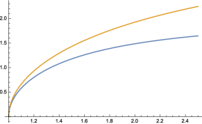
kurtosis $\gamma_{2}(c)$

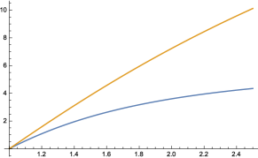
Figure 12: Comparison between the skewness and the kurtosis measures for the time-causal kernels corresponding to the limit case of $K$ first-order integrators coupled in cascade when the number of temporal scale levels $K$ tends to infinity (blue curves) and the corresponding temporal kernels in Koenderink’s scale-time model (brown curves) with the parameter values determined such that the first- and second-order temporal moments are equal (equation (164)).

Figure 12 shows an additional quantification of the differences between these two classes of temporal smoothing kernels by showing how the skewness and the kurtosis measures vary as function of the distribution parameter $c$ for the same mapping (164) between the parameters in the two families of temporal smoothing kernels. As can be seen from the graphs, both the skewness and the kurtosis measures are higher for the kernels in Koenderink’s scale-time model compared to our time-causal kernels corresponding to first-order integrators coupled in cascade and do in these respect correspond to a larger deviation from a Gaussian behaviour over the temporal domain. (Recall that for a purely Gaussian temporal model all the cumulants of higher order than two are zero, including the skewness and the kurtosis measures.)

Appendix C Scale invariance and covariance of scale-normalized temporal derivatives based on the limit kernel

In this appendix we will show that in the special case when the temporal scale-space concept is given by convolution with the limit kernel according to (39) and (LABEL:eq-FT-comp-kern-log-distr-limit), the corresponding scale-normalized derivatives by either variance-based normalization (76) or $L_{p}$-normalization (77) are perfectly scale invariant for temporal scaling transformations with temporal scaling factors $S$ that are integer powers of the distribution parameter $c$. As a pre-requisite for this result, we start by deriving the transformation property of scale-normalized derivatives by $L_{p}$-normalization (77) under temporal scaling transformations.

C.1 Transformation property of $L_{p}$-norms of scale-normalized temporal derivative kernels under temporal scaling transformations

By differentiating the transformation property (44) of the limit kernel under scaling transformations for $S=c^{j}$

$$\Psi(t;\;\tau,c)=c^{j}\Psi(c^{j}\,t;\;c^{2}j\tau,c)$$ (176)

we obtain

$$\Psi_{t^{n}}(t;\;\tau,c)=c^{j}c^{nj}\Psi_{t^{n}}(c^{j}\,t;\;c^{2}j\tau,c)=c^{j(n+1)}\Psi_{t^{n}}(c^{j}\,t;\;c^{2}j\tau,c).$$ (177)

The $L_{p}$-norm of the $n$:th-order derivative of the limit kernel at temporal scale $\tau=c^{2j}$

$$\|\Psi_{t^{n}}(\cdot;\;c^{2}j,c)\|_{p}^{p}=\int_{u=0}^{\infty}\left|\psi_{t^{n}}(u;\;c^{2}j,c)\right|^{p}$$ (178)

can then by the change of variables $u=c^{j}z$ with $du=c^{j}dz$ and using the transformation property (177) be transformed to the $L_{p}$-norm at temporal scale $\tau=1$ according to

$$\begin{split}\|\psi_{t^{n}}(\cdot;\;c^{2}j,c)\|_{p}^{p}&=\left(\int_{z=0}^{\infty}\left|c^{-j(n+1)}\Psi_{t^{n}}(z;\;1,c)\right|^{p}dz\right)c^{j}\end{split}$$

$$\begin{split}&=c^{-j(n+1)p+j}\|\psi_{t^{n}}(\cdot;\;1,c)\|_{p}^{p}\end{split}$$ (179)

thus implying the following transformation property over scale

$$\|\psi_{t^{n}}(\cdot;\;c^{2}j,c)\|_{p}=c^{-j(n+1)+j/p}\|\psi_{t^{n}}(\cdot;\;1,c)\|_{p}.$$ (180)

Thereby, the scale normalization factors for temporal derivatives in equation (LABEL:eq-sc-norm-der-Lp-norm-2)

$$\begin{split}\alpha_{n,\gamma}(c^{2j})&=\frac{G_{n,\gamma}}{\|h_{t^{n}}(\cdot;\;c^{2j})\|_{p}}=c^{j(n+1)-j/p}\,\frac{G_{n,\gamma}}{\|\psi_{t^{n}}(\cdot;\;1,c)\|_{p}}\end{split}$$

$$\begin{split}&=c^{j(n+1)-j/p}\,N_{n,\gamma}\end{split}$$ (181)

evolve in a similar way over temporal scales as the scaling factors of variance-based normalization (76) for $\tau=c^{2j}$

$$\tau^{n\gamma/2}=c^{jn\gamma}$$ (182)

if and only if

$$p=\frac{1}{1+n(1-\gamma)}.$$ (183)

C.2 Transformation property of scale-normalized temporal derivatives under temporal scaling transformations

Consider two signals $f$ and $f^{\prime}$ that are related by a temporal scaling transform $f^{\prime}(t^{\prime})=f(t)$ for $t^{\prime}=c^{j^{\prime}-j}t$ according to (46)

$$L^{\prime}(t^{\prime};\;\tau^{\prime},c)=L(t;\;\tau,c)$$ (184)

between corresponding temporal scale levels $\tau^{\prime}=c^{2(j^{\prime}-j)}\tau$. By differentiating (184) and with $\partial_{t}=c^{j^{\prime}-j}\partial_{t^{\prime}}$ we obtain

$$c^{n(j^{\prime}-j)}L_{t^{\prime n}}(t^{\prime};\;\tau^{\prime},c)=L_{t^{n}}(t;\;\tau,c).$$ (185)

Specifically, for any temporal scales $\tau^{\prime}=c^{2j^{\prime}}$ and $\tau=c^{2j}$ we have

$$c^{nj^{\prime}}L_{t^{\prime n}}(t^{\prime};\;c^{2j^{\prime}},c)=c^{nj}L_{t^{n}}(t;\;c^{2j},c).$$ (186)

This implies that for the temporal scale-space concept defined by convolution with the limit kernel, scale-normalized derivatives computed with scale normalization factors defined by either $L_{p}$-normalization (LABEL:eq-sc-norm-factor-Lp-norm-limit-kernel) for $p=1$ or variance-based normalization (182) for $\gamma=1$ will be equal

$$L^{\prime}_{\zeta^{\prime n}}(t^{\prime};\;\tau^{\prime},c)=L_{\zeta^{n}}(t;\;\tau,c)$$ (187)

between matching scale levels under temporal scaling transformations with temporal scaling factors $S=c^{j^{\prime}-j}$ that are integer powers of the distribution parameter $c$.

More generally, for $L_{P}$-normalization for any value of $p$ with a corresponding $\gamma$-value according to (183) it holds that

$$\begin{split}L^{\prime}_{\zeta^{\prime n}}(t^{\prime};\,\tau^{\prime},c)&=\alpha_{n,\gamma}(\tau^{\prime})\,L^{\prime}_{t^{\prime n}}(t^{\prime};\;\tau^{\prime},c)=\left\{\mbox{eq. (\ref{eq-sc-norm-factor-Lp-norm-limit-kernel})}\right\}\end{split}$$

$$\begin{split}&=c^{j^{\prime}(n+1)-j^{\prime}/p}\,N_{n,\gamma}\,L^{\prime}_{t^{\prime n}}(t^{\prime};\,c^{nj^{\prime}},c)=\left\{\mbox{eq. (\ref{eq-rel-p-gamma-temp-scsp-limit-kernel})}\right\}\end{split}$$

$$\begin{split}&=c^{j^{\prime}n\gamma}\,N_{n,\gamma}\,L^{\prime}_{t^{\prime n}}(t^{\prime};\,c^{nj^{\prime}},c)\end{split}$$

$$\begin{split}&=c^{j^{\prime}n(\gamma-1)}\,N_{n,\gamma}\,c^{j^{\prime}n}L^{\prime}_{t^{\prime n}}(t^{\prime};\,c^{nj^{\prime}},c)=\left\{\mbox{eq. (\ref{eq-sc-cov-sc-norm-limit-ker-der-p1-gamma1-spec})}\right\}\end{split}$$

$$\begin{split}&=c^{j^{\prime}n(\gamma-1)}\,N_{n,\gamma}\,c^{jn}L_{t^{n}}(t;\,c^{nj},c)\end{split}$$

$$\begin{split}&=c^{(j^{\prime}-j)n(\gamma-1)}\,c^{jn\gamma}\,N_{n,\gamma}\,L_{t^{n}}(t;\,c^{nj},c)\end{split}$$

$$\begin{split}&=c^{(j^{\prime}-j)n(\gamma-1)}\,c^{j(n+1)-j/p}\,N_{n,\gamma}\,L_{t^{n}}(t;\,c^{nj},c)\end{split}$$

$$\begin{split}&=c^{(j^{\prime}-j)n(\gamma-1)}\,\alpha_{n,\gamma}(\tau)\,L_{t^{n}}(t;\;\tau,c)\end{split}$$

$$\begin{split}&=c^{(j^{\prime}-j)n(\gamma-1)}\,L_{\zeta^{n}}(t;\,\tau,c)=\left\{\mbox{eq. (\ref{eq-rel-p-gamma-temp-scsp-limit-kernel})}\right\}\end{split}$$

$$\begin{split}&=c^{(j^{\prime}-j)(1-1/p)}\,L_{\zeta^{n}}(t;\,\tau,c)\end{split}$$ (188)

In the proof above, we have for the purpose of calculations related the evolution properties over scale relative to the temporal scale $\tau=1$ and normalized the relative strengths between temporal derivatives of different order to the corresponding strengths $G_{n,\gamma}$ of $L_{p}$-norms of Gaussian derivates. These assumptions are however not essential for the scaling properties and corresponding scaling transformations can be derived relative to any other temporal base level $\tau_{0}$ as well as for other ways of normalizing the relative strengths of scale-normalized derivatives between different orders $n$ and distribution parameters $c$.

References

- (1) Adelson, E., Bergen, J.: Spatiotemporal energy models for the perception of motion. J. Optical Society of America A 2, 284–299 (1985)
- (2) Alvarez, L., Guichard, F., Lions, P.L., Morel, J.M.: Axioms and fundamental equations of image processing. Arch. for Rational Mechanics 123(3), 199–257 (1993)
- (3) Babaud, J., Witkin, A.P., Baudin, M., Duda, R.O.: Uniqueness of the Gaussian kernel for scale-space filtering. IEEE Trans. Pattern Analysis and Machine Intell. 8(1), 26–33 (1986)
- (4) Barbieri, D., Citti, G., Cocci, G., Sarti, A.: A cortical-inspired geometry for contour perception and motion integration. Journal of Mathematical Imaging and Vision 49(3), 511–529 (2014)
- (5) Barnsley, M.F., Devaney, R.L., Mandelbrot, B.B., Peitgen, H.O., Saupe, D., Voss, R.F.: The Science of Fractals. Springer, New York (1988)
- (6) Barnsley, M.F., Rising, H.: Fractals Everywhere. Academic Press (1993)
- (7) van der Berg, E.S., Reyneke, P.V., de Ridder, C.: Rotational image correlation in the Gauss-Laguerre domain. In: Third SPIE Conference on Sensors, MEMS and Electro-Optic Systems: Proc. of SPIE, vol. 9257, pp. 92,570F–1–92,570F–17 (2014)
- (8) den Brinker, A.C., Roufs, J.A.J.: Evidence for a generalized Laguerre transform of temporal events by the visual system. Biological Cybernetics 67(5), 395–402 (1992)
- (9) Cocci, C., Barbieri, D., Sarti, A.: Spatiotemporal receptive fields in V1 are optimally shaped for stimulus velocity estimation. Journal of the Optical Society of America (JOSA A) 29(1), 130–138 (2012)
- (10) Daubechies, I.: Ten Lectures on Wavelets. SIAM, Philadelphia (1992)
- (11) DeAngelis, G.C., Anzai, A.: A modern view of the classical receptive field: Linear and non-linear spatio-temporal processing by V1 neurons. In: L.M. Chalupa, J.S. Werner (eds.) The Visual Neurosciences, vol. 1, pp. 704–719. MIT Press (2004)
- (12) DeAngelis, G.C., Ohzawa, I., Freeman, R.D.: Receptive field dynamics in the central visual pathways. Trends in Neuroscience 18(10), 451–457 (1995)
- (13) Duits, R., Burgeth, B.: Scale spaces on Lie groups. In: F. Gallari, A. Murli, N. Paragios (eds.) Proc. Int. Conf. on Scale-Space Theories and Variational Methods in Computer Vision (SSVM 2007), Lecture Notes in Computer Science, vol. 4485, pp. 300–312. Springer (2007)
- (14) Duits, R., Felsberg, M., Florack, L., Platel, B.: -scale-spaces on a bounded domain. In: L. Griffin, M. Lillholm (eds.) Proc. Scale-Space Methods in Computer Vision (Scale-Space’03), Lecture Notes in Computer Science, vol. 2695, pp. 494–510. Springer, Isle of Skye, Scotland (2003)
- (15) Duits, R., Florack, L., de Graaf, J., ter Haar Romeny, B.: On the axioms of scale space theory. J. of Mathematical Imaging and Vision 22, 267—298 (2004)
- (16) Fagerström, D.: Temporal scale-spaces. Int. J. of Computer Vision 2–3, 97–106 (2005)
- (17) Fagerström, D.: Spatio-temporal scale-spaces. In: F. Gallari, A. Murli, N. Paragios (eds.) Proc. Int. Conf. on Scale-Space Theories and Variational Methods in Computer Vision (SSVM 2007), Lecture Notes in Computer Science, vol. 4485, pp. 326–337. Springer (2007)
- (18) Faugeras, O., Toubol, J., Cessac, B.: A constructive mean-field analysis of multi-population neural networks with random synaptic weights and stochastic inputs. Frontiers in Computational Neuroscience 3(1), 10.3389/neuro.10.001.2009 (2009)
- (19) Felsberg, M., Sommer, G.: The monogenic scale-space: A unifying approach to phase-based image processing in scale-space. J. of Mathematical Imaging and Vision 21, 5–26 (2004)
- (20) Fleet, D.J., Langley, K.: Recursive filters for optical flow. IEEE Trans. Pattern Analysis and Machine Intell. 17(1), 61–67 (1995)
- (21) Florack, L.M.J.: Image Structure. Series in Mathematical Imaging and Vision. Springer (1997)
- (22) Florack, L.M.J., ter Haar Romeny, B.M., Koenderink, J.J., Viergever, M.A.: Families of tuned scale-space kernels. In: G. Sandini (ed.) Proc. European Conf. on Computer Vision (ECCV’92), Lecture Notes in Computer Science, vol. 588, pp. 19–23. Springer-Verlag, Santa Margherita Ligure, Italy (1992)
- (23) Florack, L.M.J., ter Haar Romeny, B.M., Koenderink, J.J., Viergever, M.A.: Scale and the differential structure of images. Image and Vision Computing 10(6), 376–388 (1992)
- (24) Fourtes, M.G.F., Hodgkin, A.L.: Changes in the time scale and sensitivity in the omatadia of limulus. Journal of Physiology 172, 239–263 (1964)
- (25) Freeman, W.T., Adelson, E.H.: The design and use of steerable filters. IEEE Trans. Pattern Analysis and Machine Intell. 13(9), 891–906 (1991)
- (26) Guichard, F.: A morphological, affine, and Galilean invariant scale-space for movies. IEEE Trans. Image Processing 7(3), 444–456 (1998)
- (27) ter Haar Romeny, B. (ed.): Geometry-Driven Diffusion in Computer Vision. Series in Mathematical Imaging and Vision. Springer (1994)
- (28) ter Haar Romeny, B., Florack, L., Nielsen, M.: Scale-time kernels and models. In: Proc. Int. Conf. Scale-Space and Morphology in Computer Vision (Scale-Space’01), Lecture Notes in Computer Science. Springer, Vancouver, Canada (2001)
- (29) Heeger, D.J.: Normalization of cell responses in cat striate cortex. Visual Neuroscience 9, 181–197 (1992)
- (30) Heil, C.E., Walnut, D.F.: Continuous and discrete wavelet transforms. SIAM review 31(4), 628–666 (1989)
- (31) Hubel, D.H., Wiesel, T.N.: Receptive fields of single neurones in the cat’s striate cortex. J Physiol 147, 226–238 (1959)
- (32) Hubel, D.H., Wiesel, T.N.: Receptive fields, binocular interaction and functional architecture in the cat’s visual cortex. J Physiol 160, 106–154 (1962)
- (33) Hubel, D.H., Wiesel, T.N.: Brain and Visual Perception: The Story of a 25-Year Collaboration. Oxford University Press (2005)
- (34) Iijima, T.: Observation theory of two-dimensional visual patterns. Tech. rep., Papers of Technical Group on Automata and Automatic Control, IECE, Japan (1962)
- (35) Jhuang, H., Serre, T., Wolf, L., Poggio, T.: A biologically inspired system for action recognition. In: International Conference on Computer Vision (ICCV’07), pp. 1–8 (2007)
- (36) Karlin, S.: Total Positivity. Stanford Univ. Press (1968)
- (37) Koch, C.: Biophysics of Computation: Information Processing in Single Neurons. Oxford University Press (1999)
- (38) Koenderink, J.J.: The structure of images. Biological Cybernetics 50, 363–370 (1984)
- (39) Koenderink, J.J.: Scale-time. Biological Cybernetics 58, 159–162 (1988)
- (40) Koenderink, J.J., van Doorn, A.J.: Receptive field families. Biological Cybernetics 63, 291–298 (1990)
- (41) Koenderink, J.J., van Doorn, A.J.: Generic neighborhood operators. IEEE Trans. Pattern Analysis and Machine Intell. 14(6), 597–605 (1992)
- (42) Laptev, I., Caputo, B., Schuldt, C., Lindeberg, T.: Local velocity-adapted motion events for spatio-temporal recognition. Computer Vision and Image Understanding 108, 207–229 (2007)
- (43) Laptev, I., Lindeberg, T.: Local descriptors for spatio-temporal recognition. In: Proc. ECCV’04 Workshop on Spatial Coherence for Visual Motion Analysis, Lecture Notes in Computer Science, vol. 3667, pp. 91–103. Springer, Prague, Czech Republic (2004)
- (44) Laptev, I., Lindeberg, T.: Velocity-adapted spatio-temporal receptive fields for direct recognition of activities. Image and Vision Computing 22(2), 105–116 (2004)
- (45) Lindeberg, T.: Scale-space for discrete signals. IEEE Trans. Pattern Analysis and Machine Intell. 12(3), 234–254 (1990)
- (46) Lindeberg, T.: Discrete derivative approximations with scale-space properties: A basis for low-level feature extraction. J. of Mathematical Imaging and Vision 3(4), 349–376 (1993)
- (47) Lindeberg, T.: Effective scale: A natural unit for measuring scale-space lifetime. IEEE Trans. Pattern Analysis and Machine Intell. 15(10), 1068–1074 (1993)
- (48) Lindeberg, T.: Scale-Space Theory in Computer Vision. Springer (1993)
- (49) Lindeberg, T.: Scale-space theory: A basic tool for analysing structures at different scales. Journal of Applied Statistics 21(2), 225–270 (1994). Also available from http://www.csc.kth.se/tony/abstracts/Lin94-SI-abstract.html
- (50) Lindeberg, T.: On the axiomatic foundations of linear scale-space. In: J. Sporring, M. Nielsen, L. Florack, P. Johansen (eds.) Gaussian Scale-Space Theory: Proc. PhD School on Scale-Space Theory, pp. 75–97. Springer, Copenhagen, Denmark (1996)
- (51) Lindeberg, T.: Linear spatio-temporal scale-space. In: B.M. ter Haar Romeny, L.M.J. Florack, J.J. Koenderink, M.A. Viergever (eds.) Scale-Space Theory in Computer Vision: Proc. First Int. Conf. Scale-Space’97, Lecture Notes in Computer Science, vol. 1252, pp. 113–127. Springer, Utrecht, The Netherlands (1997)
- (52) Lindeberg, T.: On automatic selection of temporal scales in time-casual scale-space. In: G. Sommer, J.J. Koenderink (eds.) Proc. AFPAC’97: Algebraic Frames for the Perception-Action Cycle, Lecture Notes in Computer Science, vol. 1315, pp. 94–113. Springer, Kiel, Germany (1997)
- (53) Lindeberg, T.: Feature detection with automatic scale selection. Int. J. of Computer Vision 30(2), 77–116 (1998)
- (54) Lindeberg, T.: Time-recursive velocity-adapted spatio-temporal scale-space filters. In: P. Johansen (ed.) Proc. European Conf. on Computer Vision (ECCV 2002), Lecture Notes in Computer Science, vol. 2350, pp. 52–67. Springer, Copenhagen, Denmark (2002)
- (55) Lindeberg, T.: Scale-space. In: B. Wah (ed.) Encyclopedia of Computer Science and Engineering, pp. 2495–2504. John Wiley and Sons, Hoboken, New Jersey (2008)
- (56) Lindeberg, T.: Generalized Gaussian scale-space axiomatics comprising linear scale-space, affine scale-space and spatio-temporal scale-space. J. of Mathematical Imaging and Vision 40(1), 36–81 (2011)
- (57) Lindeberg, T.: A computational theory of visual receptive fields. Biological Cybernetics 107(6), 589–635 (2013)
- (58) Lindeberg, T.: Generalized axiomatic scale-space theory. In: P. Hawkes (ed.) Advances in Imaging and Electron Physics, vol. 178, pp. 1–96. Elsevier (2013)
- (59) Lindeberg, T.: Invariance of visual operations at the level of receptive fields. PLOS ONE 8(7), e66,990 (2013)
- (60) Lindeberg, T.: Scale selection properties of generalized scale-space interest point detectors. J. of Mathematical Imaging and Vision 46(2), 177–210 (2013)
- (61) Lindeberg, T.: Image matching using generalized scale-space interest points. Journal of Mathematical Imaging and Vision 52(1), 3–36 (2015)
- (62) Lindeberg, T.: Separable time-causal and time-recursive spatio-temporal receptive fields. In: Proc. Scale-Space and Variational Methods for Computer Vision (SSVM 2015), Lecture Notes in Computer Science, vol. 9087, pp. 90–102. Springer (2015)
- (63) Lindeberg, T.: Time-causal and time-recursive spatio-temporal receptive fields. Tech. rep. (2015). ArXiv preprint arXiv:1504.02648
- (64) Lindeberg, T., Akbarzadeh, A., Laptev, I.: Galilean-corrected spatio-temporal interest operators. In: Int. Conf. on Pattern Recognition, pp. I:57–62. Cambridge (2004)
- (65) Lindeberg, T., Bretzner, L.: Real-time scale selection in hybrid multi-scale representations. In: L. Griffin, M. Lillholm (eds.) Proc. Scale-Space Methods in Computer Vision (Scale-Space’03), Lecture Notes in Computer Science, vol. 2695, pp. 148–163. Springer, Isle of Skye, Scotland (2003)
- (66) Lindeberg, T., Fagerström, D.: Scale-space with causal time direction. In: Proc. European Conf. on Computer Vision (ECCV’96), Lecture Notes in Computer Science, vol. 1064, pp. 229–240. Springer, Cambridge, UK (1996)
- (67) Lindeberg, T., Friberg, A.: Idealized computational models of auditory receptive fields. PLOS ONE 10(3), e0119,032:1–58 (2015)
- (68) Lindeberg, T., Friberg, A.: Scale-space theory for auditory signals. In: Proc. Scale-Space and Variational Methods for Computer Vision (SSVM 2015), Lecture Notes in Computer Science, vol. 9087, pp. 3–15. Springer (2015)
- (69) Lindeberg, T., Gårding, J.: Shape-adapted smoothing in estimation of 3-D depth cues from affine distortions of local 2-D structure. Image and Vision Computing 15, 415–434 (1997)
- (70) Mahmoudi, S.: Linear neural circuitry model for visual receptive fields. Tech. rep. (2015). Preprint at http://eprints.soton.ac.uk/375838/
- (71) Mallat, S.G.: A Wavelet Tour of Signal Processing. Academic Press (1999)
- (72) Mandelbrot, B.B.: The Fractal Geometry of Nature. W H Freeman and Co. (1982)
- (73) Mattia, M., Guidice, P.D.: Population dynamics of interacting spiking neurons. Physics Review E 66(5), 051,917 (2002)
- (74) Miao, X., Rao, R.P.N.: Learning the Lie group of visual invariance. Neural Computation 19, 2665–2693 (2007)
- (75) Misiti, M., Misiti, Y., Oppenheim, G., Poggi, J.M. (eds.): Wavelets and Their Applications. ISTE Ltd. (2007)
- (76) Omurtag, A., Knight, B.W., Sirovich, L.: On the simulation of large populations of neurons. Journal of Computational Neuroscience 8, 51–63 (2000)
- (77) Pauwels, E.J., Fiddelaers, P., Moons, T., van Gool, L.J.: An extended class of scale-invariant and recursive scale-space filters. IEEE Trans. Pattern Analysis and Machine Intell. 17(7), 691–701 (1995)
- (78) Perona, P.: Steerable-scalable kernels for edge detection and junction analysis. Image and Vision Computing 10, 663–672 (1992)
- (79) Rivero-Moreno, C.J., Bres, S.: Spatio-temporal primitive extraction using Hermite and Laguerre filters for early vision video indexing. In: Image Analysis and Recognition, Springer LNCS, vol. 3211, pp. 825–832 (2004)
- (80) Sato, K.I.: Lévy Processes and Infinitely Divisible Distributions. Cambridge Studies in Advanced Mathematics. Cambridge University Press (1999)
- (81) Schoenberg, I.J.: Über Variationsvermindernde Lineare Transformationen. Mathematische Zeitschrift 32, 321–328 (1930)
- (82) Schoenberg, I.J.: Contributions to the problem of approximation of equidistant data by analytic functions. Quarterly of Applied Mathematics 4, 45–99 (1946)
- (83) Schoenberg, I.J.: On totally positive functions, Laplace integrals and entire functions of the Laguerre-Pòlya-Schur type. Proc. National Academy of Sciences 33, 11–17 (1947)
- (84) Schoenberg, I.J.: Some analytical aspects of the problem of smoothing. In: Courant Anniversary Volume, Studies and Essays, pp. 351–370. New York (1948)
- (85) Schoenberg, I.J.: On Pòlya frequency functions. ii. Variation-diminishing integral operators of the convolution type. Acta Sci. Math. (Szeged) 12, 97–106 (1950)
- (86) Schoenberg, I.J.: On smoothing operations and their generating functions. Bull. Amer. Math. Soc. 59, 199–230 (1953)
- (87) Schoenberg, I.J.: I. J. Schoenberg Selected Papers, vol. 2. Springer (1988). Edited by C. de Boor
- (88) Shabani, A.H., Clausi, D.A., Zelek, J.S.: Improved spatio-temporal salient feature detection for action recognition. In: British Machine Vision Conference (BMVC’11), pp. 1–12. Dundee, U.K. (2011)
- (89) Simoncelli, E.P., Freeman, W.T., Adelson, E.H., Heeger, D.J.: Shiftable multi-scale transforms. IEEE Trans. Information Theory 38(2) (1992)
- (90) Tschirsich, M., Kuijper, A.: Notes on discrete Gaussian scale space. J. of Mathematical Imaging and Vision 51, 106–123 (2015)
- (91) U. Sharma, U., Duits, R.: Left-invariant evolutions of wavelet transforms on the similitude group. Applied and Computational Harmonic Analysis (2014)
- (92) Valois, R.L.D., Cottaris, N.P., Mahon, L.E., Elfer, S.D., Wilson, J.A.: Spatial and temporal receptive fields of geniculate and cortical cells and directional selectivity. Vision Research 40(2), 3685–3702 (2000)
- (93) Weickert, J.: Anisotropic Diffusion in Image Processing. Teubner-Verlag, Stuttgart, Germany (1998)
- (94) Weickert, J., Ishikawa, S., Imiya, A.: On the history of Gaussian scale-space axiomatics. In: J. Sporring, M. Nielsen, L. Florack, P. Johansen (eds.) Gaussian Scale-Space Theory: Proc. PhD School on Scale-Space Theory, pp. 45–59. Springer, Copenhagen, Denmark (1997)
- (95) Weickert, J., Ishikawa, S., Imiya, A.: Linear scale-space has first been proposed in Japan. J. of Mathematical Imaging and Vision 10(3), 237–252 (1999)
- (96) Willems, G., Tuytelaars, T., van Gool, L.: An efficient dense and scale-invariant spatio-temporal interest point detector. In: Proc. European Conf. on Computer Vision (ECCV 2008), Lecture Notes in Computer Science, vol. 5303, pp. 650–663. Springer, Marseille, France (2008)
- (97) Witkin, A.P.: Scale-space filtering. In: Proc. 8th Int. Joint Conf. Art. Intell., pp. 1019–1022. Karlsruhe, Germany (1983)
- (98) Yuille, A.L., Poggio, T.A.: Scaling theorems for zero-crossings. IEEE Trans. Pattern Analysis and Machine Intell. 8, 15–25 (1986)
- (99) Zelnik-Manor, L., Irani, M.: Event-based analysis of video. In: Proc. Computer Vision and Pattern Recognition, pp. II:123–130. Kauai Marriott, Hawaii (2001)