Extended-soft-core Baryon-Baryon ESC08 model
III. Hyperon-hyperon/nucleon Interactions
Abstract
This paper presents the Extended-Soft-Core (ESC) potentials ESC08c
for baryon-baryon channels with total strangeness .
The potential models for are
based on SU(3) extensions of potential models for the and
sectors, which are fitted to experimental data.
Flavor SU(3)-symmetry is broken only ’kinematically’ by the masses
of the baryons and the mesons.
For the S=-2 channels no experimental scattering data exist, and
also the information from hypernuclei is rather limited.
Nevertheless, in the fit to the and sectors information from the
NAGARA event and the -well-depth has been used as constraints to determine
the free parameters in the simultaneous fit of the data.
Therefore, the potentials for the sectors are mainly determined
by the NN-, YN-data, and SU(3)-symmetry.
Various properties of the potentials are illustrated by giving results
for scattering lengths, bound states, phase-parameters,
and total cross sections.
Notably is the prediction of a bound state in the
-channel with a binding energy MeV.
This state is ”deuteron-like” i.e. a member of the -decuplet.
As for the normal deuteron the strong tensor force is
responsible for this state.
The features of hypernuclei predicted by ESC08c are studied on the basis
of the G-matrix approach. The well-depth MeV and the
conversion width is MeV.
pacs:
13.75.Cs, 12.39.Pn, 21.30.+ypacs:
13.75.Ev, 12.39.Pn, 21.30.-xI Introduction
In this paper, the third in a series of papers following NRY12a ; NRY12b , henceforth referred to as I and II respectively, on the results and predictions of the Extended-soft-core (ESC) model for low energy baryon-baryon interactions. It presents the next phase in the development of the ESC-models and is the follow up of the ESC04-models Rij05 ; RY05 ; Rij05b and the ESC08a,b-models YMR10a for . In SR99 the Nijmegen soft-core one-boson-exchange (OBE) interactions NSC97a-f for baryon-baryon (BB) systems for were presented.
For the S=-2 YY and YN channels hardly any experimental scattering information is available, and also the information from hypernuclei is very limited. There are data on double -hypernuclei, which recently became very much improved by the observation of the Nagara-event Tak01 . This event indicates that the -interaction is rather weak, in contrast to the estimates based on the older experimental observations Dan63 ; Pro66 .
In the absense of experimental scattering information, we assume that
the potentials obey (broken) flavor SU(3) symmetry. As in I and II,
the potentials are parametrized in terms of meson-baryon-baryon,
and meson-pair-baryon-baryon couplings and gaussian form factors
as well as diffractive couplings.
This enables us to include in the interaction one-boson-exchange (OBE),
two-pseudoscalar-exchange (TME), and meson-pair-exchange (MPE),
and diffractive contributions without any new parameters.
All parameters have been fixed by a simultaneous
fit to the NN and YN data, with the constraints
imposed (i) for from the NAGARA event, and
(ii) for the well-depth . The latter is assumed to be attractive and is the
main reason for the occurrence of the ”deuteron-like” state in the ESC08-model.
For the procedure see the description in I and II.
This way, each -model
leads to a YY-model in a well defined way, and the predictions for
the - and -channels contain no ad hoc free parameters.
We have choosen for ESC08c the options:
SU(3)-symmetry for of coupling constants, and pseudovector coupling for the
pseudoscalar mesons.
(In ESC04 also alternative options were investigated, but it appeared that there is no reason
to choose any of these.)
Then, SU(3)-symmetry allows us to define all coupling constants
needed to describe the multi-strange interactions
in the baryon-baryon channels occurring in .
Quantum-chromodynamics (QCD) is, as is generally accepted now, the physical basis
of the strong interactions. Since in QCD the gluons are flavor blind, SU(3)-symmetry
is a basic symmetry, which is broken by the chiral-symmetry-breaking at
low energies. This picture supports our assumptions, stated above, on SU(3)-symmetry.
As is shown in Rij05 ; RY05 the coupling constants and the -ratio’s
used in the ESC04-models follow the predictions of the -pair creation
model (QPC) Mic69 rather closely.
The same is the case for the ESC08-models, see paper I and
Ref. THAR11 for details.
Now, it has been shown that in the
strong-coupling Hamiltonian lattice formulation of QCD, the flux-tube model, that
this is indeed the dominant picture in flux-tube breaking Isg85 .
Therefore, since the ESC-models are very much in line with the Quark-model and QCD,
the predictions for the -channels should be rather realistic.
The material in this paper is organized by the following considerations:
Most of the details of the SU(3) description are well known. In particular
for baryon-baryon scattering the details can be found in papers I, II, and e.g.
MRS89 ; RSY99 ; SR99 . Here we restrict ourselves to a minimal
exposition of these matters that is necessary for the readability of this paper.
Therefore, in Sec. II
we first review for the baryon-baryon multi-channel description, and
present the SU(3)-symmetric interaction Hamiltonian describing
the interaction vertices between mesons and members of the
baryon octet, and define their coupling
constants. We then identify the various channels which
occur in the baryon-baryon systems.
In appendix A the potentials on the isospin basis are given in terms
of the SU(3)-irreps.
In most cases, the
interaction is a multi-channel interaction, characterized by transition
potentials and thresholds. Details were given in SR99 ; RSY99 .
For the details on the pair-interactions,
we refer to paper I and II NRY12a ; NRY12b .
In Sec. III we give a general treatment of the problem
of flavor-exchange forces, which is very helpful to understand
the proper treatment of exchange forces and the treatment
of baryon-baryon channels with identical particles.
In Sec. V we describe briefly the treatment of the
multi-channel threshods in the potentials.
In Sec. VI we present the results of the ESC08c
potentials for all the sectors with total strangeness .
We give the couplings and -ratio’s for OBE-exchanges of ESC08c.
Similarly, tables with the pair-couplings are shown in appendix B.
We give the -wave scattering lengths, discuss the possibility of
bound states in these partial waves. Also, we give the S-matrix information for the
elastic channels in terms of the Bryan-Klarsfeld-Sprung (BKS) phase parameters
Bry81 ; Kla83 ; Spr85 , or in the Kabir-Kermode (KK) Kab87 format.
Tables with the BKS-phase parameters are displayed in appendix C.
Such information is very useful for example for the
construction of the -, -, and -nucleus potentials.
We also give results for the total cross sections for all leading channels.
Important differences among the different versions of the ESC-models appear in the sectors. Table XXV in Ref. RY05 demonstrates that ESC04a,b (ESC04c,d) lead to repulsive (attractive) potentials in nuclear matter. In ESC08c, and also ESC08a/b/a” YMR10b , the interactions is attractive enough to produce various hypernuclei. A notable advantage of ESC08 over ESC04 is the occurrence of a ”deuteron-like” bound state in the I=1 channel, which is accessible in a -transition -production experiment at JPARC. Therefore, it is very interesting to study the ESC08 interactions in the G-matrix approach to baryonic matter. In Sec. VII, we represent the G-matrix interactions derived from ESC08c as density-dependent local potentials. Here, structure calculations for hypernuclei are performed with use of -nucleus folding potentials obtained from the G-matrix interactions. It is discussed how the features of ESC08c appear in the level structure of hypernuclei. We conclude the paper with a summary and some final remarks in Sec. VIII.
II Channels, Potentials, and SU(3) Symmetry
II.1 Multi-channel Formalism
In this paper we consider the baryon-baryon reactions with
| (1) |
Like in Ref.’s MRS89 ; RSY99 we will for the YN-channels also refer to and as particles 1 and 3, and to and as particles 2 and 4. For the kinematics and the definition of the amplitudes, we refer to paper I Rij05 of this series. Similar material can be found in MRS89 . Also, in paper I the derivation of the Lippmann-Schwinger equation in the context of the relativistic two-body equation is described.
On the physical particle basis, there are five charge channels:
| (2) |
Like in MRS89 ; RSY99 , the potentials are calculated on the isospin basis. For hyperon-nucleon systems there are three isospin channels:
| (3) |
For the kinematics of the reactions and the various thresholds, see RSY99 . In this work we do not solve the Lippmann-Schwinger equation, but the multi-channel Schrödinger equation in configuration space, completely analogous to MRS89 . The multi-channel Schrödinger equation for the configuration-space potential is derived from the Lippmann-Schwinger equation through the standard Fourier transform, and the equation for the radial wave function is found to be of the form MRS89
| (4) |
where contains the potential, nonlocal contributions, and the centrifugal barrier, while is only present when non-local contributions are included. The solution in the presence of open and closed channels is given, for example, in Ref. Nag73 . The inclusion of the Coulomb interaction in the configuration-space equation is well known and included in the evaluation of the scattering matrix.
Obviously, the potential on the particle basis for the and channels are given by the potential on the isospin basis. For and , the potentials are related to the potentials on the isospin basis by an isospin rotation. Using the indices for , and respectively, we have Mae95
| (5) |
and for we have
| (6) |
Here, when necessary an isospin label is added in parentheses.
The momentum space and configuration space potentials for the ESC-model have been described in Rij05 for baryon-baryon in general. Therefore, they apply also to hyperon-nucleon and we can refer for that part of the potential to paper I. Also in the ESC-model, the potentials are of such a form that they are exactly equivalent in both momentum space and configuration space. The treatment of the mass differences among the baryons are handled exactly similar as is done in MRS89 ; RSY99 . Also, exchange potentials related to strange meson exchanhes etc. , can be found in these references.
The baryon mass differences in the intermediate states for TME- and MPE- potentials has been neglected for YN-scattering. This, although possible in principle, becomes rather laborious and is not expected to change the characteristics of the baryon-baryon potentials.
II.2 Potentials and SU(3) Symmetry
We consider all possible baryon-baryon interaction channels, where the baryons are the members of the baryon octet
| (7) |
The baryon masses, used in this paper, are given in Table 5. The meson nonets can be written as
| (8) |
where the singlet matrix has elements on the diagonal, and the octet matrix is given by
| (9) |
and where we took the pseudoscalar mesons with as a specific example. For the other mesons the octet matrix is obtained by the following substitutions: (i) vector mesons , , , (ii) scalar , , , (iii) axial-vector , , .
Introducing the following notation for the isodoublets,
| (18) |
the most general, SU(3) invariant, interaction Hamiltonian is then given by Swa63
| (19) | |||||
where we again took the pseudoscalar mesons as an example, dropped the Lorentz character of the interaction vertices, and introduced the charged-pion mass to make the pseudovector coupling constant dimensionless. All coupling constants can be expressed in terms of only four parameters. The explicit expressions can be found in Ref. RSY99 . The -hyperon is an isovector with phase chosen such Swa63 that
| (20) |
This definition for differs from the standard Condon and Shortley phase convention Con35 by a minus sign. This means that, in working out the isospin multiplet for each coupling constant in Eq. (19), each entering or leaving an interaction vertex has to be assigned an extra minus sign. However, if the potential is first evaluated on the isospin basis and then, via an isospin rotation, transformed to the potential on the physical particle basis (see below), this extra minus sign will be automatically accounted for.
In appendix A, Table 16 and Table 17 we give the relation between the potentials on the isospin-basis, see (5)-(6), and the SU(3)-irreps.
Given the interaction Hamiltonian (19) and a theoretical scheme for deriving the potential representing a particular Feynman diagram, it is now straightforward to derive the one-meson-exchange baryon-baryon potentials. We follow the Thompson approach Tho70 ; Rij91 ; Rij92 ; Rij96 and expressions for the potential in momentum space can be found in Ref. MRS89 . Since the nucleons have strangeness , the hyperons , and the cascades , the possible baryon-baryon interaction channels can be classified according to their total strangeness, ranging from for to for . Apart from the wealth of accurate scattering data for the total strangeness sector, there are only a few, and not very accurate, scattering data for the sector, while there are no data at all for the sectors. We therefore believe that at this stage it is not yet worthwhile to explicitly account for the small mass differences between the specific charge states of the baryons and mesons; i.e., we use average masses, isospin is a good quantum number, and the potentials are calculated on the isospin basis. The possible channels on the isospin basis are given in (3).
However, the Lippmann-Schwinger or Schrödinger equation is solved for the physical particle channels, and so scattering observables are calculated using the proper physical baryon masses. The possible channels on the physical particle basis can be classified according to the total charge ; these are given in (2). The corresponding potentials are obtained from the potential on the isospin basis by making the appropriate isospin rotation. The matrix elements of the isospin rotation matrices are nothing else but the Clebsch-Gordan coefficients for the two baryon isospins making up the total isospin. (Note that this is the reason why the potential on the particle basis, obtained from applying an isospin rotation to the potential on the isospin basis, will have the correct sign for any coupling constant on a vertex which involves a .)
In order to construct the potentials on the isospin basis, we need first the matrix elements of the various OBE exchanges between particular isospin states. Using the iso-multiplets (9) and the Hamiltonian (19) the isospin factors can be calculated. The results are given in Table 1, where we use the pseudoscalar mesons as a specific example. The entries contain the flavor-exchange operator , which is for a flavor symmetric and for a flavor anti-symmetric two-baryon state. Since two-baryons states are totally anti-symmetric, one has . Therefore, the exchange operator has the value for even- singlet and odd- triplet partial waves, and for odd- singlet and even- triplet partial waves. In order to understand Table 1 fully, we have given in the following section Sec. III a general treatment of exchange forces. This treatment shows also how to deal with the case where the initial/final state involves identical particles and the final/inition state does not.
Second, we need to evaluate the TME and the MPE exchanges. The method we used for these is the same as for hyperon-nucleon, and is described in RY05 , Sec. IID.
III Exchange Forces
The proper treatment of the flavor-exchange forces is for the -channels more difficult than for the -channels. The extra complication is the occurrence of couplings between channels with identical and channels with non-identical particles. In order to understand the several -factors, see SR99 , we give here a systematic treatment of the flavor-exchange potentials. The method followed is using a multi-channel framework, which starts starts by ordering the two-particle states by assigning and for the channel labeled with the index , like in eq. (1). The particles and have CM-momenta and , spin components and . The two-baryon states and are considered to be distinct, leading to distinct two-baryon channels. The ’direct’ and the ’exchange’ T-amplitudes are given by the T-matrix elements
| (21) |
and similarly for the direct and flavor-exchange potentials and . It is obvious from rotation invariance that
| (22) |
A similar definition (21) and relation (22) apply for the direct and flavor-exchange potentials and .
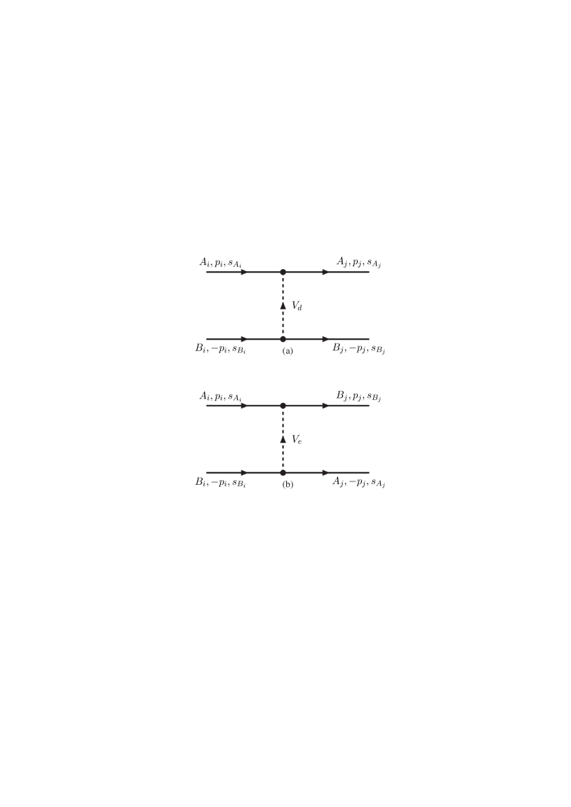
We notice that in interchanging A and B there is no exchange of momenta or spin-components, see Fig. 2. This is necessary for the application of Lippmann-Schwinger type of integral equations, which can produce only one type of spectral function e.g. . So, the momentum transfer for and for is the same. Viewed from the coupled-channel scheme this is the standard situation.
The integral equations with two-baryon unitarity, e.g. the Thompson-, Lippmann-Schwinger-equation etc., read for the - and -operator
| (23a) | |||||
| (23b) | |||||
These coupled equations can be diagonalized by introducing the T±- and V±-operators
| (24) |
which, as follows from (23), satisfy separate integral equations
| (25) |
Notice that on the basis of states with definite flavor symmetry
| (26) |
the and matrix elements are also given by
| (27) |
III.1 Identical Particles
Sofar, we considered the general case where for all channels. In the case that for some , one has , because there is no distinct physical state corresponding to the ’flavor exchange-state’. For example for a flavor single channel like one deduces from (23) that then also , and one has in this case the integral equation
| (28) |
where the labels and now denote e.g. the spin-components.
III.2 Coupled and system
This multi-channel system represents the case where there is mixture of channels with identical and with non-identical particles. The three states we distinguish are , and . Choosing the same ordering, the potential written as a -matrix reads
| (29) |
With a similar notation for the T-matrix, the Lippmann-Schwinger equation can be written compactly as a -matrix equation:
| (30) |
Next, we make a transformation to states, which are either symmetric or anti-symmetric for particle interchange. Then, according to the discussion above, we can separate them in the Lippmann-Schwinger equation. This is achieved by the transformation
| (31) |
one gets in the transformed basis for the potential
| (32) |
and of course, a similar form is obtained for the T-matrix on the transformed basis. Now, obviously we have that and . Therefore, one sees that the even and odd states under particle exchange are decoupled in (32). Also , etc. showing the appearance of the -factors, mentioned before. Indeed, they appear in a systematic way using the multi-channel framework.
III.3 The K-exchange Potentials
Consider for example the -system, having . Mesons with strangeness, i , , , , , are obviously the only ones that can give transition potentials, i.e. and . The -states anti-symmetric and symmetric in flavor are respectively:
| (33a) | |||
| (33b) | |||
Analyzing the -state one has because of the anti-symmetry of the two-fermion state w.r.t. the exchange of all quantum labels, , where denotes the flavor-symmetry. Taking here the as a generic example, and using (18) and (19), one finds that
| (34) | |||||
| (35) |
Then, since , one obtains for the ’direct’ potential the coupling
| (36) |
The same result is found for the ’exchange’ potential . Therefore
| (37) | |||||
which has indeed the -factor given in Table 1, and is identical to Table IV in SR99 , for .
For the entry for consists of two parts. These correspond to and respectively, i.e. the direct and exchange contributions involve different couplings. Therefore, they are not added together.
III.4 The - and -exchange Potentials
Next, we discuss briefly the calculation of the entries for - and -exchange in Table 1. First, the entries with — indicate that the corresponding physical state does not exist. Next we give further specific remarks and calculations:
-
a.
For -exchange one has that . The matrix elements for the - and -state are easily seen to be correct. For the -states one has for , and for . This explains the matrix element.
-
b.
For the calculation is identical to that for NN, in particular .
-
c.
For consider the and matrix elements. In these cases one has as one can easily check. Then, using the cartesian base, we have for . Employing the states and , one obtains the results in Table 1.
With the ingredients given above one can easily check the other entries in Table 1.
| — | ||
| 1 | ||
| — | 1 | |
| 1 | ||
| — | ||
| — | ||
| — | ||
| — | ||
| — |
IV Short-range Phenomenology
For a detailed discussion and description of the short-range region we refer to paper II NRY12b . Here, the meson- and diffractive-exchange and the quark-core in the ESC08c-modeling has been described. In this section we give the quark-core phenomenology for the S=-2 baryon-baryon channels.
IV.1 Relation S=-2 YN,YY-states and SUfs(6)-irreps
The relation between the SUf(3)-irreps and SUfs(6)-irreps has been derived in paper II NRY12b In Appendix A the S=-2 BB-potentials are given in terms of the SU(3)f-irreps. Combining these two things gives the representation of the S=-2 potentials in terms of the SUfs(6)-irreps as displayed in Tables 2 and 3.
IV.2 Parametrization Quark-core effects
As introduced in II, the repulsive short-range Pomeron-like YN,YY potential is splitted linearly in a diffractive (Pomeron) and a quark-core component by writing
| (38) |
where represents the genuine Pomeron and the structural effects of the quark-core forbidden [51]-configuration, i.e. a Pauli-blocking (PB) effect. Since the Pomeron is a unitary-singlet its contribution is the same for all BB-channels (apart from some small baryon mass breaking effects), i.e. . Furthermore the PB-effect for the BB-channels is assumed to be proportional to the relative weight of the forbidden [51]-configuration compared to its weight in NN
| (39) |
where denotes the quark-core fraction w.r.t. the pomeron potential for the NN-channel, i.e. . Then we have
| (40) |
on the spin,isospin basis.
A subtle treatment of BB channels according to this linear scheme is characteristic for the ESC08c-model. The value of the PB factor is searched in the fit to the NN- and YN-data. The parameter turns out to be about 27.5%. This means that the Quark-core repulsion is roughly 34% of the genuine Pomeron repulsion. Then, the PB effects in the S=-2 channels are entirely determined. From Eqn. (40) the ratio is given by the weights of the [51]-irrep and . In Table 4 we give this ratio for the various S=-2 BB channels in the ESC08c model, With only one exception, the effective pomeron repulsion is stronger than in the NN-channels.
V Multi-channel Thresholds and Potentials
V.1 Thresholds
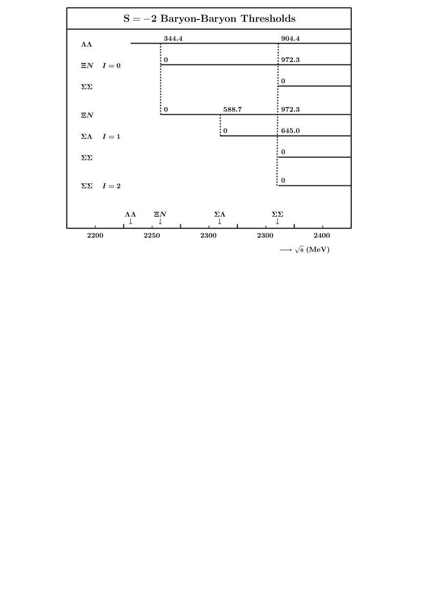
Clearly, the two-baryon channels represent a number of separate coupled-channel systems, separated by the charge, see (2). A further subdivision is according to the total isospin. The different thresholds have been discussed in detail in SR99 , and we show these thresholds here in Fig. 1 for the purpose of general orientation. Their presence turns the Lippmann-Schwinger and Schrödinger equation into a coupled-channel matrix equation, where the different channels open up at different energies. In general one has a combination of ’open’ and ’closed’ channels. For a discussion of the solution of such a mixed system, we refer to Swa71 .
V.2 Threshold- and Meson-mass corrections in Potentials
As discussed in SR99 , the one-meson-exchange Feynman-graph consists actually of two three-dimensional time-ordered graphs. The energy denominator from these two diagrams reads
| (41) |
where, is the total energy and , with the meson mass and the momentum transfer. From (41) it is clear that the potential is energy dependent. We use the static approximation and , where the superscript 0 refers to the masses of the lowest threshold of the particular coupled-channel system q, see (2). They are in general not equal to the masses and occurring in the time-ordered diagrams. For example, the potential for the contribution in the coupled-channel system has , but . Denoting , and similarly for , we have for the ’propagators’ Rij92 for
| (42) |
For there is the extra term
on the r.h.s. in (42).
This integral representation makes it possible to deal with it numerically
rather exactly. However, we think that such a sophistication is unnecessary
at present nor for a description of the scattering data, nor for .
where there are virtually no data at all.
Therefore, we handle with this energy dependence approximately as follows:
1. Elastic potentials: In this case we use (42), and in (41) one has and , for the elastic channel, label . Here . Then,
| (43) | |||||
for .
Because of this condition we can not apply this to the pseudoscalars,
but is possible for the vector-, scalar-, and axial-mesons.
The largest effect is for -scattering,
where the -channel potential is somewhat reduced by this effect.
This because the -channel is rather far away from the others.
In this paper we neglect the effects of a finite
in all elastic channels and for all mesons.
2. Inelastic potentials: In this case, like in SR99 and all other papers on the Nijmegen potentials, we use the approximation of Swa62 , using the fact that is mostly rather close to the average of the initial and final-sate baryon masses. Then, the propagator can be written as
| (44) |
which amounts to introducing an effective meson mass
| (45) |
For more details of this effect on the exchanged meson masses, we refer to SR99 .
| Baryon | Mass | |
|---|---|---|
| Nucleon | 938.2796 | |
| 939.5731 | ||
| Hyperon | 1115.60 | |
| 1189.37 | ||
| 1192.46 | ||
| 1197.436 | ||
| Cascade | 1314.90 | |
| 1321.32 |
VI Results
The main purpose of this paper is to present the properties of the ESC08c potentials for the sector. As described above, the free parameters in each model are fitted mainly to the and scattering data for the and sectors, respectively. Given the expressions for the coupling constants in terms of the octet and singlet parameters and their values for the six different models as presented in Ref. RSY99 , it is straightforward to evaluate all possible baryon-baryon-meson coupling constants needed for the potentials. A complete set of coupling constants for models ESC08c is given in Table 6.
In Fig’s 3 and Fig. 4 we display the OBE potentials for the individual pseudoscalar, vector, scalar, and axial mesons in the case of model ESC08c.
| 0.2687 | 0.1961 | 0.1970 | –0.0725 | –0.2683 | 0.0714 | 0.0725 | –0.2687 | |||
| 0.6446 | 1.2892 | 0.0000 | 0.6446 | –1.1165 | 1.1165 | –0.6446 | –0.6446 | |||
| 3.7743 | 3.5639 | 2.3006 | –0.2104 | –4.2367 | 1.9362 | 0.2104 | –3.7743 | |||
| –0.7895 | –0.4929 | –0.6271 | 0.2967 | 0.7404 | –0.1133 | –0.2967 | 0.7895 | |||
| –0.8192 | –0.5114 | –0.6507 | 0.3078 | 0.7683 | –0.1175 | –0.3078 | 0.8192 | |||
| 0.5852 | 1.1705 | 0.0000 | 0.5852 | –1.0137 | 1.0137 | –0.5852 | –0.5852 | |||
| –1.3743 | –1.0991 | –0.9523 | 0.2746 | 1.4280 | –0.4758 | –0.2746 | 1.3743 | |||
| 0.00000 | 0.00000 | 0.00000 | 0.00000 | 0.00000 | 0.00000 | 0.00000 | 0.00000 | |||
| 0.1265 | –0.1349 | 0.2490 | –0.2045 | 0.2309 | 0.2912 | 0.2026 | 0.3073 | |||
| 3.4570 | 2.7589 | 2.7589 | 2.0608 | –1.3390 | –2.2103 | –2.2103 | –3.0816 | |||
| –0.8574 | –3.5064 | –0.6296 | –4.7170 | 3.1678 | –0.1386 | 3.4522 | –1.6497 | |||
| –0.7613 | –0.1942 | –1.1549 | –0.1074 | 0.7311 | 1.2070 | 0.4008 | 1.2798 | |||
| –0.4467 | 0.1418 | –0.8551 | 0.2319 | 0.3495 | 0.8433 | 0.4008 | 1.2798 | |||
| 4.1461 | 3.5609 | 3.5609 | 2.9758 | –1.6898 | –2.5176 | –2.5176 | –3.3453 | |||
| –0.2277 | 0.5968 | –0.5030 | 0.8714 | –0.4221 | 0.7443 | –0.8109 | 1.1331 | |||
| 3.5815 | 3.5815 | 3.5815 | 3.5815 | 0.0000 | 0.0000 | 0.0000 | 0.0000 | |||
| 4.6362 | 4.6362 | 4.6362 | 4.6362 | |||||||
| –4.7602 | –4.7602 | –4.7602 | –4.7602 |
In the following we will present the model predictions for scattering lengths, bound states, and cross sections.


VI.1 Effective-range parameters
For ESC08c the low-energy parameters are
| -threshold | -threshold | |||
|---|---|---|---|---|
| 11 | 0.472 | 13.001 | 0.062 | 11.774 |
| 12 | 1.591 | 2.088 | –1.436 | 9.744 |
| 22 | 0.870 | 3.276 | –0.736 | 9.659 |
| ESC08c | ||
|---|---|---|
| 11 | 1.302 | 1.454 |
| 12 | –9.122 | 18.305 |
| 13 | 0.504 | 1.709 |
| 22 | 239.128 | –590.173 |
| 23 | 4.252 | –16.637 |
| 33 | 1.030 | 1.540 |
For we have for ESC08c:
and for we have for ESC08c:
The values in parentheses indicate the values without Coulomb. The results at the threshold and at the threshold are given in Table 7-8. The scattering lengths are found to be larger in absolute value than in the NSC97 models SR99 , indicating a more attractive interaction.
The old experimental information seemed to indicate a separation energy of MeV, corresponding to a rather strong attractive interaction. As a matter of fact, an estimate for the scattering length, based on such a value for , gives fm Tan65 ; Bod65 . However, in recent years the experimental information and interpretation of the ground state levels of He, Be, and B Dal89 , has been changed drastically. This because of the Nagara-event Tak01 , identified uniquely as He Tak01 , which established that the -interaction is weaker ( MeV).
In NSC97 RSY99 it was only possible to increase the attraction in the channel by modifying the scalar-exchange potential. If the scalar mesons are viewed as being mainly states, one finds that the (attractive) scalar-exchange part of the interaction in the various channels satisfies
| (46) |
suggesting indeed a rather weak -potential. The NSC97 fits to the scattering data RSY99 give values for the scalar-meson mixing angle which seem to point to almost ideal mixing for the scalars as states. We found that an increased attraction in the channel would give rise to (experimentally unobserved) deeply bound states in the channel. On the other hand, in the ESC-models there are in principle more possibilities because of the presence of meson-pair potentials. As one sees from the values of the in the ESC08c model of this paper, we can produce the apparently required attraction in the interaction without giving rise to bound states. Notice that also in ESC08 we have ideal scalar mixings, akin to NSC97.
| Space-spin symmetric | |||
|---|---|---|---|
| Channels | SU(3)-irreps | ||
| 0 | 0 | ||
| –1 | 1/2 | , | , |
| 3/2 | |||
| –2 | 0 | ||
| 1 | , | , , | |
| , | |||
| Space-spin antisymmetric | |||
| Channels | SU(3)-irreps | ||
| 0 | 1 | ||
| –1 | 1/2 | , | , |
| 3/2 | |||
| –2 | 0 | , , | , , |
| 1 | , | , | |
| 2 | |||

VI.2 Deuteron state in
A discussion of the possible bound-states, using the SU(3) content of the different channels is given in SR99 . As in SR99 , for a general orientation, we list in Table 9 all the irreps to which the various baryon-baryon channels belong. In ESC08c we find a deuteron with isospin I=1 and strangeness S=-2, belonging to the SU(3)-irrep, which is a bound state in the - coupled partial wave. In model ESC04d Rij05b , however, there occurs a bound state in the - partial wave. From Table 9 one sees that this is a -state, which was a little bit surprising, because the OBE-potential one expects to be rather repulsive in the irrep , see MRS89 . In the ESC04 models this occurrence was ascribed to the inclusion of the potentials of the axial-vector-mesons, and the meson pairs. Since ESC04a-c did not show such a bound state it is considered to be accidental. However, the situation in ESC08c is completely different. Here the bound state is in the deuteron-like states where strong tensor forces are present, which causes the binding similarly to the np-deuteron. In Fig. 17 the tensor potentials are shown, where it appears that also the tensor potential is important. This is similar to the situation in below the -threshold where a large cusp occurs. The calculated binding energy MeV.


VI.3 Partial Wave Phase Parameters
For the BB-channels below the inelastic threshold we use for the parametrization of the amplitudes the standard nuclear-bar phase shifts SYM57 . The information on the elastic amplitudes above thresholds is most conveniently given using the BKS-phases Bry81 ; Kla83 ; Spr85 . For uncoupled partial waves, the elastic BB -matrix element is parametrized as
| (47) |
For coupled partial waves the elastic BB-amplitudes are -matrices. The BKS -matrix parametrization, which is of the type-S variety, is given by
| (48) |
where
| (49) |
and is a real, symmetric matrix parametrize as
| (50) |
From the various parametrizations of the -matrix, we choose the Kabir-Kermode parametrization Kab87 to represent the -matrix in the figures. Then, the -matrix is given by the inelasticity parameters , called -parameters, as follows
| (51) |
where
| (52) |
Here
| (53) |
In Fig’s 13-16 the BKS-phases and coupling parameters for ESC08c are shown. In Fig 13 and Fig. 15 we also show the -phases (n.c.) for the case with no coupling to the other two-particle channels. For the n.c.-curve shows that the potential is repulsive, which is mainly due to the -irrep. The attraction comes in particular from the coupling to the -channel.
VI.4 Total cross sections
We next present the predictions for the total cross section for several channels. We suppose always that the beam as well as the target are unpolarized. Therefore, we incuded the statistical factors, which are for the spin-singlet and for the spin-triplet case.
For those cases where both baryons are charged, we do not include the purely Coulomb contribution to the total cross section, nor do we include the Coulomb interference to the nuclear amplitude. The cross section is calculated by summing the contributions from partial waves with orbital angular momentum up to and including . We find this to be sufficient for all the sectors; inclusion of any higher partial waves has no significant effect. Inclusion of higher partial waves will shift the total cross section to slightly higher values without changing the overall shape. Of course, their inclusion would be necessary if a detailed comparison with real experimental data were to be made.
In Table 10 we show the total X-sections as a function of the laboratory momentum . Being dominantly S-wave, there is in principle has a (sharp) cusp at the -threshold, i.e. MeV/, which indeed is visible in the table. In Table 10 we also show the total X-sections as a function of the laboratory momentum . In Table 11 we show the total X-sections for the and the reactions as a function of the laboratory momentum .
| 10 | 22.65 | — | 630.95 | 2468.24 |
|---|---|---|---|---|
| 50 | 20.98 | — | 114.35 | 1817.61 |
| 100 | 16.83 | — | 49.78 | 990.75 |
| 200 | 8.58 | — | 100.01 | 607.52 |
| 300 | 5.16 | — | 58.81 | 405.65 |
| 350 | 6.42 | 2.28 | 28.35 | 161.84 |
| 400 | 6.96 | 6.68 | 16.15 | 85.65 |
| 500 | 11.03 | 23.39 | 10.96 | 55.60 |
| 600 | 6.26 | 17.50 | 8.86 | 41.69 |
| 700 | 4.92 | 12.78 | 8.13 | 33.69 |
| 800 | 4.87 | 10.40 | 7.68 | 29.07 |
| 900 | 5.41 | 9.05 | 6.93 | 27.48 |
| 1000 | 5.69 | 7.38 | 6.51 | 26.94 |
| 10 | 66.52 | — | 690.58 | 10.61 | — |
| 50 | 66.55 | — | 124.73 | 8.51 | — |
| 100 | 66.75 | — | 58.40 | 6.83 | — |
| 200 | 67.88 | — | 20.46 | 10.28 | — |
| 300 | 69.36 | — | 13.78 | 17.53 | — |
| 400 | 70.27 | — | 12.96 | 21.97 | — |
| 500 | 69.80 | — | 11.86 | 36.62 | — |
| 600 | 86.79 | 2.21 | 11.70 | 42.12 | — |
| 700 | 50.02 | 3.84 | 10.19 | 19.67 | 0.99 |
| 800 | 46.79 | 5.59 | 9.84 | 15.49 | 1.94 |
| 900 | 42.87 | 6.58 | 8.67 | 26.72 | 6.32 |
| 950 | 40.71 | 7.18 | 7.58 | 23.74 | 5.60 |
| 1000 | 45.79 | 6.37 | 7.56 | 49.80 | 7.83 |
VI.5 Flavor SU(3)-irrep potentials


The solid lines show averages of the SU(3)-irrep potentials using the potentials on the particle basis. The dashed lines are the irrep potentials in an SU(3) limit, where MeV, MeV, MeV, and MeV. Comparison with the results from LQCD Inou11 ; Inou12 shows qualitatively very similar results. The exception is the SU(3)-singlet -irrep. Here LQCD potential is atractive for , whereas in ESC08c there is an attractive pocket for fm and is repulsive for fm. This shape is due to the behavior of the spin-spin potentials from pseudoscalar and vector exchange, which have zero volume integrals. In the -irrep for the SU(3)-broken potential (solid line) there is no bound state, i.e. no H-particle Jaffe77 . This is in agreement with the recent experimental result studying -decay Kim13 .
VII G-matrix interaction and -nucleus states 111 In this section we denote isospin by T, the nuclear physics notation.
We calculate potential energies and derive G-matrix interactions in nuclear matter with the use of ESC08c. G-matrix calculations are performed with the continuous (CON) choice, where off-shell potentials are taken into account continuously from on-shell ones in intermediate propagations of correlated pairs. Then, a two-body state is specified by spin , isospin , orbital and total angular momenta and , respectively. The imaginary parts of G-matrices appear due to energy-conserving transitions from to channels in the and states. The conversion width is obtained from the imaginary part of multiplying by .
| 1.4 | 8.0 | 0.3 | 1.8 | 1.4 | 2.1 | |||
| 10.7 | 11.1 | 1.1 | 0.7 | 2.6 | 0.0 | 7.0 | 4.5 |
Table 12 shows the potential energy and its partial-wave contributions at normal density . The values turn out to be given by the strong cancellation between attractive contributions in () states and repulsive contributions in () states. Eventually, values of become far less attractive than those of . The calculated value of is also given in the Table 12, the dominant contribution of which comes from the -- coupling interaction in the state.

In Fig. 22, values and partial-wave contributions are drawn as a function of . Here, is shown by a bold curve, and contributions in , , and states are shown by thin curves. -state contribution summed for states is shown by a dashed curve.
As well as in Table 12, we see here the cancellation between attractive contributions in spin-triplet states and repulsive ones in spin-singlet states. Especially, the attraction in the state is due to the -- tensor-coupling interactions in this state. If these tensor parts in this channel are switched off, the value of becomes strongly repulsive. On the other hand, the -state contributions are small.
It should be noted that the curve becomes substantially attractive in the low density region due to the strong density dependence. This feature works favorably for binding energies in light systems.
For applications to finite systems, - central parts of the complex G-matrix interactions for ESC08c are represented in Gaussian forms, whose coefficients are given as a function of . The determined parameters are given in Table 13.
| (fm) | 0.50 | 0.90 | 2.00 | |
| a | 540.0 | 5.59 | ||
| b | 4975. | 0.0 | ||
| c | 2500. | 0.0 | ||
| a | 4353. | 562.8 | 0.215 | |
| b | 6760. | 1065. | 0.0 | |
| c | 2456. | 408.9 | 0.0 | |
| a | 0.0 | 70.88 | 5.59 | |
| b | 0.0 | 3.319 | 0.0 | |
| c | 0.0 | 8.351 | 0.0 | |
| a | 0.0 | 0.215 | ||
| b | 0.0 | 0.0 | ||
| c | 0.0 | 0.0 | ||
| a | 343.9 | 111.2 | 0.357 | |
| b | 133.5 | 18.08 | 0.0 | |
| c | 10.00 | 23.38 | 0.0 | |
| a | 809.8 | 50.29 | 1.76 | |
| b | 1619. | 213.5 | 0.0 | |
| c | 633.3 | 95.44 | 0.0 | |
| a | 0.0 | 42.44 | 0.357 | |
| b | 0.0 | 1.531 | 0.0 | |
| c | 0.0 | 8.844 | 0.0 | |
| a | 0.0 | 17.26 | 1.76 | |
| b | 0.0 | 8.867 | 0.0 | |
| c | 0.0 | 6.355 | 0.0 |
As demonstrated in Ref. Yam10 , the observed spectra of hypernuclei are described successfully with the -nucleus folding potentials derived from the G-matrix interactions. Here, the same method is applied to -nucleus systems. A -nucleus folding potential in a finite system is obtained from as follows:
| (54) |
| (58) | |||||
where denote parity quantum numbers. Here, core nuclei are assumed to be spherical, and densities and mixed densities are obtained from Skyrme-HF wave functions. The isospin-dependence of leads to the Lane term. In this work, only the diagonal parts of the term are taken into account.
For included in , we use the averaged-density approximation (ADA): An averaged value of is defined by by using a -state function . Then, an averaged value of is given by . This value is put into and determined self-consistently for each state, and is a parameter fixed by a fine tuning to the experimental data. Hereafter, we investigate the two cases of and .
| C | |||
|---|---|---|---|
| 5.18 | 3.83 | ||
| 1.77 | 1.49 | ||
| 2.93 | 3.34 | ||
| 1.10 | 0.68 | ||
| 0.75 | 0.44 | ||
| 5.37 | 7.54 | ||
| N | |||
| 6.30 | 4.82 | ||
| 2.15 | 1.87 | ||
| 2.85 | 3.18 | ||
| 1.85 | 1.22 | ||
| 1.11 | 0.77 | ||
| 4.50 | 5.66 |
Table 14 shows the results for and bound states in C and N systems, where Coulomb interactions between and 12C (14N) are taken into account. and are the binding energy and r.m.s. radius of , respectively. Conversion widths come from the imaginary parts included in and states. The obtained states become unbound, when the Coulomb interactions between and 12C (14N) are switched off. Namely these states are so called Coulomb-assisted bound states. They are specified by the fact that the values of are large due to their weak binding, but far smaller than those in atomic states. For instance, we have =0.175 MeV and =36 fm for the +14N state.
Experimental information for interactions can be obtained from emulsion events of simultaneous emission of two hypernuclei (twin hypernuclei) from a absorption point. The produced by the reaction is absorbed into a nucleus (12C, 14N or 16O in emulsion) from some atomic orbit, and by the following process two hypernuclei are produced. Then, the energy difference between the initial state and the final twin state gives rise to the binding energy between and the nucleus.
Two events of twin hypernuclei (I) Aoki93 and (II) Aoki95 were observed in the KEK E-176 experiment, and recently the new event (III) Nakazawa has been observed in the KEK E373 experiment. In the cases of (I) and (II), each event has no unique interpretation for its reaction process. However, it is possible to find a consistent understanding for these two events as follows: The events (I) and (II) were interpreted to be reactions of captured by 12C. Assuming that the is absorbed from the orbit in each case, we have consistently the following reactions
Assuming that the is captured from a state, the calculated values of in the C system (1.10 and 0.68 MeV for 0.0 and 0.1, respectively) turn out to be consistent with the values of MeV given by these data. In Ref. Ehime , this result was used to fit the strength of the interaction. In these two events, however, a possibility cannot be ruled out that they are captured from states.
The event (III) is uniquely identified as
| (60) |
with MeV, which is the first clear evidence of a deeply bound state of the system. This value can be reproduced by taking , assuming the is captured from the state. However, it is far more probable that Be is produced in some excited state. In Ref. Nakazawa , the excitation energies are taken from the theoretical calculations Hiyama12 Millener12 , while the ground-state value of is taken from the emulsion data. Their estimated values of are MeV and MeV, when Be is in the first and second excited state, respectively. Our calculated values of 1.85 and 1.22 MeV for and 0.1 are within the former and the latter regions, respectively. The similar value of was predicted in Ref. Ehime . Thus, assuming that the is in a state, the experimental values of can be explained reasonably by small tuning of our G-matrix interaction in both cases of possible two excitations of Be. It should be noted that, assuming captures from states, we could get a consistent interpretation for the three emulsion events (I), (II) and (III) with use of the G-matrix interaction derived from ESC08c,
It is well known that capture probabilities of from states are far smaller than those from states. In spite of this fact, twin hypernuclei are produced dominantly after - captures. As discussed in Ref. Yam94 , the reason is because sticking probabilities of two ’s produced after - captures are substantially larger than those after - captures.
| Mg | 7.35 | 0.13 | 6.65 | 1.66 | 3.16 | |
| 3.86 | 0.08 | 0.91 | 4.32 | |||
| 0.92 | 0.03 | 0.24 | 9.47 | |||
| Sr | 15.5 | 0.63 | 13.0 | 1.85 | 3.25 | |
| 11.9 | 0.52 | 11.4 | 1.16 | 4.23 | ||
| 8.61 | 0.41 | 0.74 | 5.04 | |||
| 5.37 | 0.30 | 0.45 | 5.98 |

Hereafter, calculations are performed using the G-matrix interactions with . Let us demonstrate the results for heavier systems Mg and Sr, being produced by reactions on 28Si and 89Y targets, respectively. In Table 15, we show calculated values of s.p. energies , conversion widths and r,m.s radii of solved wave functions, where and are contributions from Lane terms and Coulomb interactions, respectively. It should be noted that the deep and states are owing to large contributions from Coulomb attractions.
The BNL-E885 experiment E885 suggests that a s.p. potential in Be is given by the attractive Wood-Saxon potential with the depth MeV (called WS14). In this case, the calculated value of is 0.41 (0.79) MeV for the C (14N) system, WS14 being slightly less attractive than the above -nucleus potentials suitable to the emulsion events of twin hypernuclei.
In order to investigate the possibility of observing hypernuclear state, we calculate spectra of reactions on some targets with use of our G-matrix folding potentials. Calculations are performed with the Green’s function method in DWIA Tadokoro . In Fig. 23, we show the obtained spectra for 12C and 28Si targets at forward-angle with an incident momentum 1.65 GeV. We can see clearly the peaks of - and -bound states, respectively, in the cases of 12C and 28Si targets. Here, the experimental resolution is assumed to be 2 MeV. Solid and dotted curves are for ESC08c and WS14, respectively. Strong enhancement of the highest- state in the ESC08c case is due to the -dependent effects of G-matrix interactions. When the values for the and states are taken as the same as those for the states, the obtained spectra for ESC08c become similar to those for WS14. We conclude this section by making some remarks on the inclusion of the three-body repulsive (TBR) and attractive (TBA) interactions for S=-2 systems. In the case of the -hypernuclei in paper II NRY12b an important conclusion from the G-matrix analysis is that the experimental values and excited spectra can be reproduced in a natural way by ESC08c. Although the multipomeron (MPP) repulsive contributions are decisively important in the high density region, they should be almost canceled by the three-body attractions (TBA) in the normal density region.
In the case of the -hypernuclei it is shown here that the attraction in ESC08c is consistent with the -nucleus binding energies given by the emulsion data of the twin -hypernuclei. As in the case of the -hypernuclei, we can expect some role of the MPP+TBA contribution. For a clear analysis, however, the experimental data of are too scarce. On the other hand, MPP contributions are essential in the problem of -mixing in neutron star matter. We defer the discussion and inclusion of the three-body interactions in the S=-2 system, i.e. ESC08c+ model, to a future paper.
VIII Summary and Conclusion
The ESC08c model potentials presented here are a major step in constructing the baryon-baryon interactions for scattering and hypernuclei in the context of broken SU(3)-symmetry using, apart from the gaussian repulsion from the Pomeron and inclusion of a systematic quark-core effects for all baryon-baryon channels, generalized yukawian meson-exchange for the dynamics. The potentials are based on (i) One-boson-exchanges, where the coupling constants at the baryon-baryon-meson vertices are restricted by the broken SU(3) symmetry, (ii) Two-pseudoscalar exchanges, (iii) Meson-Pair exchanges. Each type of meson exchange (pseudoscalar, vector, axial-vector, scalar) contains five free parameters: a singlet coupling constant, an octet coupling constant, the ratio , a meson-mixing angle. The potentials are regularized with gaussian cut-off parameters, which provide a few additional free parameters. As shown in paper I and II the parameters could be restricted, both for OBE and MPE, by the Quark-model predictions in the form of the quark-antiquark creation mechanism.
Although we performed truly simultaneous fits to the NN and YN data,
effectively
most of these parameters are determined in fitting the rich and
accurate NN scattering data, while the remaining ones are fixed
by fitting also the (few) YN scattering data. This still leaves
enough flexibility to accomodate the imposition of a few extra constraints.
As demonstrated here, the assumption of SU(3) symmetry for the couplings then
allows us to extend these models to the higher strangeness channels
(i.e., YY and all interactions involving cascades), without the
need to introduce additional free parameters.
Like the NSC97 models, the ESC04 and ESC08 models are very powerful models
of this kind, and the very first realistic ones.
The most striking prediction of ESC08c is the existence of the S=-2
deuteron , below the -threshold.
The width is expected to be small since the decay must be isospin
breaking and is electromagnetic and/or weak. The experimental search for
baryon-baryon bound states by the Rome-Saclay-Vanderbilt collaboration
RSV82 in the mass range 21.-2.5 GeV/c was negative.
It could be that the resolution in this experiment was insufficient
to detect a very narrow state near the -threshold.
It is important to emphasize that the existence of the -state is strongly
connected to the -nucleus attraction as indicated by experiments,
see E885 and the recent emulsion-experiments results Nakazawa .
In one of the ESC04-models, ESC04d, the bound S=-2 bound state occurred
in the -channel,
which is a member of an SU(3) octet -irrep. The ESC08c result
is much more natural, fitting nicely with the existence of a
SU(3)-deuteron multiplet.
In order to illustrate the basic properties of these potentials, we have presented results for scattering lengths, possible bound states in -waves, and total cross sections. Although the different versions ESC04 and ESC08 produce the and data well, there are considerable differences. In the NN-sector the quality of the fit to the NN-data of the ESC08-models is superior to that for the ESC04-models. Also, they lead to notable differences in the hypernuclear structures, especially in systems. A typical example can be seen in their sectors: The derived -nucleus potentials are different from each other even qualitatively. It is quite important that ESC04d and ESC08a,b,c solutions predicts the existence of -hypernuclei consistently with the indication given by the BNL-E885 experiment. For a discussion -nucleus attraction in the case of the ESC04 and ESC08a,b we refer to Rij05b and YMR10b respectively. The -nucleus attraction derived from ESC08c is owing to the situation that the interaction in the () state is substantially attractive. This feature is intimately related to tensor-potential giving a strong Lane term. The mass dependence of hypernuclei predicted by ESC08c is rather different from that by the OBE model such as NHC-D. The most striking is that the peculier hypernuclear states are obtained by ESC08c even in - and light -shell regions.
We finally mention that these ESC08 potentials also provide an excellent starting point for calculations and predictions of multi-strange systems. The extension of this work to the -systems, i.e. comprising all baryon-baryon states, will be the topic of the last paper (IV) in this series.
Acknowledgements.
We thank T. Motoba and E. Hiyama for many stimulating discussions.Appendix A Baryon-baryon channels and SU(3)-irreps
In Table 16 and Table 17 we give the relation between the potentials on the isospin basis and the potentials in the SU(3)-irreps.
| Space-spin antisymmetric states | ||
| ,, | ||
| ,, | ||
| ,, | ||
| ,, | ||
| ,, | ||
| ,, | ||
| ,, | ||
on the isospin basis.
| Space-spin symmetric states | ||
|---|---|---|
Appendix B Meson-pair coupling constants
In Table 18 we give the MPE-couplings for model ESC08c.
| Pair | Type | ||||||||||||
|---|---|---|---|---|---|---|---|---|---|---|---|---|---|
| –1.2371 | –2.4742 | 0.0000 | –1.2371 | 2.1427 | –2.1427 | 1.2371 | 1.2371 | ||||||
| –2.1427 | 0.0000 | 0.0000 | 2.1427 | ||||||||||
| 0.2703 | 0.5406 | 0.0000 | 0.2703 | –0.4682 | 0.4682 | –0.2703 | –0.2703 | ||||||
| 0.4682 | 0.0000 | 0.0000 | –0.4682 | ||||||||||
| –1.6592 | –1.3274 | –1.1495 | 0.3318 | 1.7243 | –0.5748 | –0.3318 | 1.6592 | ||||||
| –0.5748 | 1.1495 | –1.1495 | 1.7243 | ||||||||||
| 5.1287 | 4.1030 | 3.5533 | –1.0257 | –5.3299 | 1.7766 | 1.0257 | –5.1287 | ||||||
| 1.7766 | –3.5533 | 3.5533 | –5.3299 | ||||||||||
| –0.2988 | –0.2391 | –0.2070 | 0.0598 | 0.3106 | –0.1035 | –0.0598 | 0.2988 | ||||||
| –0.1035 | 0.2070 | –0.2070 | 0.3106 | ||||||||||
| –0.2059 | –0.1648 | –0.1427 | 0.0412 | 0.2140 | –0.0713 | –0.0412 | 0.2059 | ||||||
| –0.0713 | 0.1427 | –0.1427 | 0.2140 |
Appendix C BKS-phase parameters
| 10 | 1.23 | — | –0.00 | — | 0.00 | — | 0.00 | 0.00 | 0.00 |
| 50 | 5.94 | — | –0.00 | — | 0.01 | — | 0.02 | 0.00 | 0.00 |
| 100 | 10.67 | — | –0.04 | — | 0.10 | — | 0.18 | 0.00 | 0.00 |
| 200 | 14.96 | — | –0.35 | — | 0.57 | — | 1.30 | 0.02 | 0.00 |
| 300 | 15.06 | — | –1.17 | — | 1.19 | — | 3.95 | 0.13 | 0.03 |
| 350 | 18.43 | 13.90 | –1.66 | 0.71 | 1.40 | 0.29 | 6.39 | 0.30 | 0.07 |
| 400 | 11.31 | 20.52 | –2.12 | 4.48 | 1.48 | 1.80 | 10.78 | 0.72 | 0.16 |
| 500 | 5.63 | 22.04 | –3.56 | 9.92 | 1.07 | 4.59 | 14.55 | 2.81 | 0.36 |
| 600 | –9.11 | 21.73 | –5.07 | 14.51 | –0.12 | 7.22 | –5.00 | 3.61 | 0.58 |
| 700 | –17.82 | 20.65 | –5.92 | 19.01 | –1.84 | 9.51 | –8.75 | 4.04 | 0.83 |
| 800 | –25.64 | 18.80 | –5.56 | 23.66 | –3.67 | 11.53 | –10.75 | 4.76 | 1.11 |
| 900 | –32.03 | 15.64 | –3.43 | 28.44 | –4.47 | 13.85 | –12.81 | 5.81 | 1.65 |
| 1000 | –36.88 | 13.35 | 0.02 | 33.25 | –7.46 | 21.89 | –14.18 | 6.75 | 1.03 |
| 10 | 0.08 | 5.45 | 0.00 | 0.00 |
|---|---|---|---|---|
| 50 | 0.25 | 11.85 | 0.05 | 0.00 |
| 100 | –0.30 | 15.88 | 0.33 | 0.00 |
| 200 | –4.17 | 19.78 | 1.23 | 0.00 |
| 300 | –10.09 | 21.40 | 1.50 | 0.00 |
| 350 | –13.37 | 21.79 | 1.22 | 0.00 |
| 400 | –16.72 | 22.00 | 0.64 | 0.00 |
| 500 | –23.34 | 22.00 | –1.31 | 0.00 |
| 600 | –29.54 | 21.56 | –4.11 | 0.00 |
| 700 | –35.03 | 20.72 | –7.50 | 0.00 |
| 800 | –39.55 | 19.44 | –11.23 | 0.00 |
| 900 | –42.78 | 17.51 | –15.13 | 0.00 |
| 1000 | –43.87 | 14.78 | –19.11 | 0.00 |
| 10 | –0.70 | — | –0.00 | — | 0.00 | — | 0.00 | 0.00 | –0.00 |
| 50 | –3.46 | — | –0.04 | — | 0.04 | — | 0.00 | 0.00 | –0.00 |
| 100 | –6.75 | — | –0.29 | — | 0.30 | — | 0.02 | 0.01 | –0.00 |
| 200 | –12.79 | — | –1.32 | — | 1.55 | — | 0.08 | 0.12 | –0.01 |
| 300 | –18.35 | — | –2.39 | — | 3.18 | — | 0.03 | 0.35 | –0.05 |
| 350 | –20.95 | — | –2.80 | — | 3.92 | — | –0.12 | 0.48 | –0.07 |
| 400 | –23.37 | — | –3.12 | — | 4.52 | — | –0.39 | 0.62 | –0.10 |
| 500 | –27.15 | — | –3.45 | — | 5.24 | — | –1.33 | 0.76 | –0.12 |
| 600 | –24.30 | 17.88 | –3.31 | 0.61 | 5.55 | 1.35 | –2.82 | 1.12 | –0.13 |
| 700 | –37.01 | 24.33 | –2.37 | 5.39 | 5.49 | 7.50 | –4.74 | 1.31 | –0.05 |
| 800 | –44.30 | 25.12 | –0.89 | 11.40 | 4.39 | 11.77 | –6.93 | 1.46 | 0.10 |
| 900 | –37.14 | 25.06 | 0.28 | 18.12 | 2.47 | 14.93 | –9.26 | 1.60 | 0.31 |
| 1000 | –31.01 | 24.57 | –0.21 | 24.24 | –0.00 | 17.31 | –11.65 | 1.73 | 0.58 |
| 10 | 0.08 | 5.45 | 6.19 | 0.00 | 0.00 | 1.00 | 0.00 | 1.00 |
|---|---|---|---|---|---|---|---|---|
| 50 | 0.25 | 11.85 | 27.52 | 0.20 | 0.00 | 1.00 | 0.00 | 1.00 |
| 100 | –0.30 | 15.88 | 42.78 | 0.87 | –0.00 | 1.00 | 0.03 | 1.00 |
| 200 | –4.17 | 19.78 | 51.04 | 2.47 | –0.08 | 0.99 | 0.11 | 0.99 |
| 300 | –10.09 | 21.40 | 49.00 | 4.48 | –0.32 | 0.98 | 0.18 | 0.98 |
| 400 | –16.72 | 22.00 | 43.88 | 7.06 | –0.87 | 0.97 | 0.24 | 0.97 |
| 500 | –23.34 | 22.00 | 37.52 | 10.12 | –1.77 | 0.95 | 0.28 | 0.95 |
| 600 | –29.54 | 21.56 | 30.65 | 13.41 | –2.81 | 0.92 | 0.29 | 0.92 |
| 700 | –35.03 | 20.72 | 23.85 | 16.71 | –3.47 | 0.90 | 0.27 | 0.90 |
| 800 | –39.55 | 19.44 | 17.52 | 19.87 | –3.32 | 0.89 | 0.23 | 0.89 |
| 900 | –42.78 | 17.51 | 11.74 | 22.77 | –2.24 | 0.89 | 0.18 | 0.89 |
| 1000 | –43.87 | 14.78 | 6.42 | 25.31 | –0.37 | 0.91 | 0.14 | 0.91 |
| 10 | –0.70 | 0.00 | 173.90 | 0.00 | –0.00 | 1.00 | –0.00 | 1.00 |
|---|---|---|---|---|---|---|---|---|
| 50 | –3.48 | 0.00 | 151.56 | 0.03 | –0.00 | 1.00 | –0.00 | 1.00 |
| 100 | –6.80 | 0.00 | 131.47 | 0.11 | –0.01 | 1.00 | –0.00 | 1.00 |
| 200 | –12.91 | 0.00 | 110.65 | 0.23 | –0.10 | 1.00 | –0.02 | 1.00 |
| 300 | –18.55 | 0.00 | 101.81 | 0.28 | –0.27 | 1.00 | –0.05 | 1.00 |
| 400 | –23.69 | 0.00 | 99.08 | 0.36 | –0.43 | 1.00 | –0.08 | 1.00 |
| 500 | –27.67 | 0.00 | 101.75 | 0.75 | –0.44 | 0.99 | –0.13 | 0.99 |
| 600 | –25.39 | 17.43 | 118.13 | 2.44 | –0.26 | 0.77 | –0.14 | 0.99 |
| 700 | –37.88 | 23.74 | 116.81 | 3.32 | 0.06 | 0.45 | –0.16 | 0.98 |
| 800 | –43.46 | 24.45 | 118.30 | 4.69 | 0.57 | 0.33 | –0.20 | 0.97 |
| 900 | –36.27 | 24.31 | 121.57 | 6.81 | 1.45 | 0.28 | –0.23 | 0.95 |
| 1000 | –30.08 | 23.74 | 131.27 | 10.53 | 2.15 | 0.34 | –0.26 | 0.93 |
| 10 | 0.32 | 6.17 | –1.42 | 0.00 | –0.00 | 1.00 | –0.00 | 1.00 |
|---|---|---|---|---|---|---|---|---|
| 50 | 1.34 | 13.32 | –7.13 | 0.07 | –0.00 | 0.88 | –0.00 | 1.00 |
| 100 | 1.43 | 17.66 | –14.35 | 0.40 | –0.04 | 0.77 | –0.00 | 1.00 |
| 200 | –1.80 | 21.80 | –28.78 | 1.09 | –0.44 | 0.60 | –0.02 | 1.00 |
| 300 | –7.51 | 23.57 | –42.69 | 1.11 | –1.16 | 0.48 | –0.03 | 1.00 |
| 400 | –14.37 | 24.31 | –55.47 | 0.85 | –1.90 | 0.39 | –0.03 | 1.00 |
| 500 | –21.64 | 24.46 | –65.61 | 1.20 | –2.31 | 0.33 | –0.07 | 0.99 |
| 600 | –28.87 | 24.18 | –67.63 | 2.90 | –1.25 | 0.31 | –0.17 | 0.97 |
| 700 | –35.84 | 23.54 | –29.29 | 13.38 | –3.45 | 0.19 | –0.16 | 0.83 |
| 800 | –42.45 | 22.62 | –6.47 | 13.61 | –9.76 | 0.19 | –0.08 | 0.87 |
| 900 | –41.35 | 21.45 | –1.81 | 11.92 | –13.71 | 0.28 | –0.07 | 0.88 |
| 1000 | –35.53 | 20.11 | –3.05 | 10.41 | –17.07 | 0.36 | –0.09 | 0.89 |
| 10 | –12.35 (0.94) | –0.20 ( 0.00) | –0.22 ( –0.00) | –0.21 ( 0.00) | 0.00 | –0.00 ( 0.00) |
|---|---|---|---|---|---|---|
| 50 | –13.72 (4.26) | –3.08 ( 0.19) | –3.41 ( –0.12) | –3.27 ( 0.01) | 0.00 | –0.01 ( 0.00) |
| 100 | –5.59 (6.46) | –6.41 ( 1.17) | –8.24 ( –0.71) | –7.44 ( 0.11) | 0.04 | –0.59 ( 0.00) |
| 200 | –3.03 (4.75) | –1.01 ( 4.46) | –8.24 ( –2.82) | –4.66 ( 0.79) | 0.43 | –3.25 ( 0.05) |
| 300 | –7.40 (–1.50) | 1.54 ( 5.86) | –9.17 ( –4.88) | –2.44 ( 1.86) | 1.07 | –2.68 ( 0.22) |
| 400 | –14.47 (–9.65) | 0.36 ( 3.95) | –10.07 ( –6.49) | –0.85 ( 2.73) | 1.63 | –2.05 ( 0.48) |
| 500 | –22.56 (–18.44) | –3.51 (–0.41) | –10.63 ( –7.53) | 0.08 ( 3.18) | 1.94 | –1.49 ( 0.76) |
| 600 | –30.91 (–27.29) | –8.89 (–6.14) | –10.59 ( –7.84) | 0.57 ( 3.31) | 1.91 | –1.10 ( 0.93) |
| 700 | –39.15 (–35.91) | –14.98(–12.50) | –9.76 ( –7.29) | 0.82 ( 3.30) | 1.56 | –1.03 ( 0.84) |
| 800 | –42.88 (–44.18) | –21.31(–19.04) | –8.14 ( –5.88) | 0.90 ( 3.17) | 0.94 | –1.36 ( 0.36) |
| 900 | –35.25 (–37.94) | –27.63(–25.53) | –5.96 ( –3.86) | 0.75 ( 2.85) | 0.15 | –2.15 (–0.54) |
| 1000 | –28.00 (–30.50) | –33.80(–31.84) | –3.57 ( –1.62) | 0.30 ( 2.25) | 0.71 | –3.37 (–1.87) |
References
- (1) M.M. Nagels, Th.A. Rijken, and Y. Yamamoto, Extended-soft-core Baryon-Baryon Model ESC08c, I. Nucleon-Nucleon Scattering , [arXiv:nucl-th/1408.4825].
- (2) M.M. Nagels, Th.A. Rijken, and Y. Yamamoto, Extended-soft-core Baryon-Baryon Model ESC08c, II. Hyperon-Nucleon Interactions, [arXiv:nucl-th/1501.06636].
- (3) Th.A. Rijken, Extended-soft-core Baryon-Baryon Model. I, Nucleon-Nucleon Interactions, Phys. Rev. C73, 044007 (2006) [arXiv:nucl-th/0603041]
- (4) Th.A. Rijken and Y. Yamamoto, Extended-soft-core Baryon-Baryon Model. II, Hyperon-Nucleon Interactions, Phys. Rev. C73, 044008 (2006) [arXiv:nucl-th/0603042]
- (5) Th.A. Rijken and Y. Yamamoto, Extended-soft-core baryon-baryon model III, hyperon-hyperon/nucleon interactions, arXiv:nucl-th/060807 (2006)
- (6) Th.A. Rijken, M.M. Nagels, and Y. Yamamoto, Progr. Theor. Phys. Suppl. 185 (2010) 14.
- (7) V.G.J. Stoks and Th.A. Rijken, Phys. Rev. C 59, 3009 (1999).
- (8) H. Takahashi, et al., Phys. Rev. Lett. 87, 212502 (2001).
- (9) M. Danysz, et al., Nucl. Phys. 49 121 (1963).
- (10) D. J. Prowse, Phys. Rev. Lett. 17 782 (1966).
- (11) L. Micu, Nucl. Phys. B10, 521 (1969); A. Le Yaouanc, L. Oliver, O. P’ene, and j.C. Raynal, Phys. Rev. D8, 2223 (1973); 9, 1415 (1974).
- (12) Th.A. Rijken, Baryon-baryonCouplings in the and QPC-models, Notes University of Nijmegen, The Netherlands, nn-online, THEF 12.01.
- (13) N. Isgur and J. Paton, Phys. Rev. D31, 2910 (1985); R. Kokoski and N. Isgur, Phys. Rev. D35, 907 (1987); T.J. Burns and F.E. Close, Phys. Rev. D74, 034003 (2006).
- (14) Th.A. Rijken, V.G.J. Stoks, and Y. Yamamoto, Phys. Rev. C 59, 21 (1999).
- (15) P.M.M. Maessen, Th.A. Rijken, and J.J. de Swart, Phys. Rev. C 40, 2226 (1989).
- (16) R.A. Bryan, Phys. Rev. C 24, 2659 (1981); 30 305 (1984).
- (17) S. Klarsfeld, Phys. Lett. 126b, 148 (1983).
- (18) D.W.L. Sprung, Phys. Rev. C 32, 699 (1985).
- (19) A. Kabir and M.W. Kermode, J.Phys.G:Nucl.Phys. 13 (1987) 501.
- (20) Y. Yamamoto, T. Motoba, and Th.A. Rijken, Progr. Theor. Phys. Suppl. 185 (2010) 72.
- (21) M.M. Nagels, T.A. Rijken, and J.J. de Swart, Ann. Phys. (N.Y.) 79, 338 (1973).
- (22) P.M.M. Maessen, private communication.
- (23) J.J. de Swart, Rev. Mod. Phys. 35, 916 (1963); 37, 326(E) (1965).
- (24) E.U. Condon and G.H. Shortley, The Theory of Atomic Spectra (Cambridge University Press, Cambridge, England, 1935).
- (25) R.H. Thompson, Phys. Rev. D 1, 110 (1970).
- (26) Th.A. Rijken, Ann. Phys. (N.Y.) 208, 253 (1991).
- (27) Th.A. Rijken and V.G.J. Stoks, Phys. Rev. C 46, 73 (1992); 46, 102 (1992).
- (28) Th.A. Rijken and V.G.J. Stoks, Phys. Rev. C 54, 2851 (1996); 54, 2869 (1996).
- (29) J.J. de Swart, M.M. Nagels, T.A. Rijken, and P.A. Verhoeven, Springer Tracts Mod. Phys. 60, 138 (1971).
- (30) J.J. de Swart and C.K. Iddings, Phys. Rev. 128, 2810 (1962); ibid 130, 319 (1963).
- (31) Y.C. Tang and B.C. Herndon, Phys. Rev. 138, B637 (1965).
- (32) A.R. Bodmer and S. Ali, Phys. Rev. 138, B644 (1965).
- (33) R.H. Dalitz, D.H. Davis, P.H. Fowler, A. Montwill, J. Pniewski, and J.A. Zakrewski, Proc. Roy. Soc. (London) A426, 1 (1989).
- (34) H.P. Stapp, T. Ypsilantis, and N. Metropolis, Phys. Rev. 105,302 (1957).
- (35) T. Inoue et al, Phys. Rev. Lett. 106 (2011) 162002.
- (36) T. Inoue et al, Nucl. Phys. A 881 (2012) 28.
- (37) R.L. Jaffe, Phys. Rev. Lett. 38 (1977) 195; 38 (1977) 617.
- (38) B.H. Kim et al, search for an H-dibaryon with mass near in decays, arXiv:1302.4028v1 [hep-ex] 17 Feb. 2013.
- (39) Y.Yamamoto, T.Motoba, Th.A. Rijken, Prog. Theor. Phys. Suppl. No.185 (2010), 72.
- (40) S. Aoki et al., Prog. Theor. Phys. 89 (1993), 493.
- (41) S. Aoki et al., Phys. Lett. B355 (1995), 45.
- (42) K. Nakazawa et al., Prog. Theor. Exp. Phys. 2015, 033D02.
- (43) M. Yamaguchi, K. Tominaga, Y. Yamamoto, and T. Ueda, Prog. Theor. Phys. 105 (2001), 627.
- (44) E. Hiyama and Y. Yamamoto, Prog. Theor. Phys. 128 (2012), 105.
- (45) D.J. Millener, Nucl. Phys. A 881 (2012), 298.
- (46) Y.Yamamoto, T.Motoba, T.Fukuda, M.Takahashi, and K.Ikeda, Prog. Theor. Phys. Suppl. No.117 (1994), 281.
-
(47)
T. Fukuda et al., Phys. Rev.C58 (1998), 1306.
P. Khaustov et al., Phys. Rev. C61 (2000), 054603. - (48) Tadokoro,S., Kobayashi,H., Akaishi,Y.: -hypernuclear states in heavy nuclei. Phys. Rev. C51, 2656-2663 (1995)
- (49) D’Agostini et al, Rome-Saclay-Vanderbilt collaboration, Nucl. Phys. B209, 1 (1982).