Spatial Distributions of Local Elastic Moduli Near the Jamming Transition

Abstract

Recent progress on studies of the nanoscale mechanical responses in disordered systems has highlighted a strong degree of heterogeneity in the elastic moduli. In this contribution, using computer simulations, we study the elastic heterogeneities in athermal amorphous solids, composed of isotropic, static, sphere packings, near the jamming transition. We employ techniques, based on linear response methods, that are amenable to experimentation. We find that the local elastic moduli are randomly distributed in space and are described by Gaussian probability distributions, thereby lacking any significant spatial correlations, that persists all the way down to the transition point. However, the shear modulus fluctuations grow as the jamming threshold is approached, which is characterized by a new power-law scaling. Through this diverging behavior we are able to identify a characteristic length scale, associated with shear modulus heterogeneities, that distinguishes between bulk and local elastic responses.

When traditional, crystalline solids are linearly deformed, their elastic responses are typically described by affine deformations Landau and Lifshitz (1986). Contrary to this, disordered solids, such as thermal amorphous solids, i.e. glasses, disordered crystals Phillips (1981), as well as athermal jammed solids Makse et al. (2000), exhibit strongly non-affine responses to elastic deformations. This non-affine character becomes significantly apparent during shear deformation Tanguy et al. (2002). Under shear, constituent particles undergo additional non-affine displacements Maloney (2006), leading to a decrease in the shear modulus from a value predicted by the affine response only Tanguy et al. (2002). It is this non-affine character that dominates the shear modulus on approach to the jamming transition, where a mechanically stable solid loses rigidity O’Hern et al. (2003); Zaccone and Scossa-Romano (2011).

The appearance of non-affine response is closely related to elastic heterogeneities Leonforte et al. (2005), especially spatially varying shear moduli. Indeed, DiDonna and Lubensky DiDonna and Lubensky (2005) proposed that non-affine displacements of particles subject to shearing are driven by randomly fluctuating local elastic moduli. Amorphous solids reflect such inhomogeneous behavior in their mechanical responses at the nanoscale Schirmacher et al. (2015a, b); Hufnagel (2015), as seen in both computer simulations Yoshimoto et al. (2004) and experiments Wagner et al. (2011). Manning and co-workers Manning and Liu (2011); Chen et al. (2011) identified soft spots as regions of atypically large displacements in low-frequency, quasi-localized vibrational modes. Particle rearrangements, activated by mechanical load Manning and Liu (2011); Tanguy et al. (2010) and by thermal energy Chen et al. (2011); Widmer-Cooper et al. (2008), are therefore understood to be spatially correlated with those soft spots, which can be linked to locally unstable regions with negative shear moduli Yoshimoto et al. (2004). Furthermore, Ellenbroek et al. Ellenbroek et al. (2006) demonstrated that the elastic response of jammed packings to local forcing fluctuates over a length scale $\ell_{\ast}$. Independently Lerner et al. Lerner et al. (2014) showed that the local elasticity is governed by a different length $\ell_{c}$. Recently Karimi and Maloney Karimi and Maloney (2015) reconciled these differing views by considering the behaviors of longitudinal and transverse components of elastic response.

Thus, it appears that spatial heterogeneities in local elastic moduli are a key feature to understanding mechanical properties of disordered solids. In this contribution, we study the elastic heterogeneities in athermal jammed solids close to the jamming transition. Specifically, we address the following points: (i) How are the local elastic moduli distributed in space? (ii) How do those distributions evolve on approach to the jamming transition? (iii) Is there a length scale over which the local elastic moduli fluctuate? For athermal systems studied here, the packing fraction $\phi$ acts as a control parameter that we use to systematically probe static packings of varying rigidity. We characterize rigidity by the distance, $\Delta\phi=\phi-\phi_{c}$, from the transition point $\phi_{c}$, or equivalently the packing pressure, $p$. The approach of $\phi_{c}$ from above ($p\rightarrow 0^{+}$) is governed by various power-law scalings with $\Delta\phi$ in quantities including global elastic moduli Makse et al. (2000); O’Hern et al. (2003); Ellenbroek et al. (2006). In the following, we unveil new power-law scalings in the spatial fluctuations of elastic moduli.

Our numerical system consists of $N$ monodisperse, frictionless spheres of diameter $\sigma$ and mass $m$, in three dimensional, periodic, cubic simulation boxes Silbert (2010). Particles interact via a finite-range, purely repulsive potential; $V(r)=(\epsilon/a)(1-r/\sigma)^{a}$ for $r<\sigma$, otherwise $V(r)=0$, where $r$ is the center-to-center separation between two particles. Here, we show results only for Hertzian contacts, $a=2.5$ jno (a). Length, mass, and time are presented in units of $\sigma$, $m$, and $\tau=(m\sigma^{2}/\epsilon)^{1/2}$. We prepared systems over several orders of magnitude in packing pressure, $10^{-7}<p<10^{-1}$, corresponding to $10^{-6}\lesssim\Delta\phi\lesssim 10^{0}$. Most of our results are for $N=1,000$, but we also show data using $N=10,000$ to probe larger length scales.

The total elastic modulus (bulk, shear), $X(=K,G)$, is obtained as a sum of the affine, $X_{A}$, and non-affine, $X_{N}$, components: $X=X_{A}-X_{N}$ Lutsko (1989); Lemaitre and Maloney (2006); Lutsko (1988); Wittmer et al. (2013); Mizuno et al. (2013a). While $X_{A}$ can be thought of as the value predicted assuming particles follow affine trajectories under an imposed deformation field, $X_{N}$ quantifies deviations from this due to non-affine relaxations. Yet, obtaining elastic modulus information in fragile systems can be problematic, especially when applying explicit deformation procedures. Here, we implemented protocols developed within linear response theory Lutsko (1989); Lemaitre and Maloney (2006); Lutsko (1988); Wittmer et al. (2013); Mizuno et al. (2013a), which avoid explicit deformation practices thereby allowing us to probe extremely close to the jamming transition.

Two protocols were employed that essentially sample the vibrational normal modes of system: (i) The zero-temperature ($T=0$) protocol (restricted to $N=1,000$) is formulated directly in terms of the dynamical matrix Lutsko (1989); Lemaitre and Maloney (2006). (ii) The finite-temperature ($T>0$) protocol (for both $N=1000$ and $N=10,000$), samples mode vibrations by switching on a small temperature ($T=10^{-9}$ to $10^{-10}$) and thermally agitating the system Lutsko (1988); Wittmer et al. (2013); Mizuno et al. (2013a). At these temperatures and $p>10^{-5}$, particle displacements are $10^{-2}$ to $10^{-4}$ $[\sigma]$, and both protocols return consistent values. Technical details of numerical procedure and formulation can be found in Supplemental Material sup . Here we highlight an important aspect of these protocols. Both procedures are accessible through current experimental technologies at the colloidal and granular scales. In particular, advances in particle tracking and resolution allow precision measurements of particle positions, used by covariance matrix analyses methods Ghosh et al. (2010); Henkes et al. (2012); Still et al. (2014), and the photo-elastic technique for particle forces Majmudar et al. (2007).

To extract local information, the simulation box was divided into small subvolumes of size $w_{x}\times w_{y}\times w_{z}$, i.e. coarse-graining (CG) domains. In each CG domain $m$, we computed the local modulus, $X^{m}=K^{m},G^{m}$, decomposed into their affine ($A$) and non-affine ($N$) components. We then calculated the probability distribution function $P(X^{m})$, from which the average $X$ and standard deviation $\delta X$ were obtained sup . $\delta X=\delta X(p,w_{x},w_{y},w_{z})$ depends on both $p$ and the size of CG domain, and quantifies the extent of fluctuations, whereas $X=X(p)$ corresponds to the global value, independent of $w_{\alpha}$ ($\alpha=x,y,z$) jno (b).

Figure 1 shows the dependence on pressure, $p$, of the moduli and their corresponding fluctuations. The global $X(p)$ are shown in the top panels, Fig. 1(a), (b), indicating that our technique is consistent with previous studies on similar systems O’Hern et al. (2003); Ellenbroek et al. (2006) that imposed explicit deformations. Since the pressure scales as $p\sim V^{\prime}\sim\Delta\phi^{a-1}$ ($\sim\Delta\phi^{1.5}$ for $a=2.5$, Hertzian contacts), the scaling laws for $X$ normalized by the effective spring constant $k_{\text{eff}}\sim V^{\prime\prime}\sim\Delta\phi^{a-2}$ Vitelli et al. (2010), $X/k_{\text{eff}}$, are consistent with:

$${K}/{k_{\text{eff}}}\sim\Delta\phi^{0},\quad{G}/{k_{\text{eff}}}\sim\Delta\phi^{0.5}.$$ (1)

The middle panels, Fig. 1(c), (d), show the absolute fluctuations, $\delta X(p,w_{x},w_{y},w_{z})$, where the CG domain is cubic of linear size, $w_{\alpha}=w\simeq 3$, and from which we find,

$${\delta K}/{k_{\text{eff}}}\sim\Delta\phi^{0},\quad{\delta G}/{k_{\text{eff}}}\sim\Delta\phi^{0.27}.$$ (2)

More importantly, the bottom panels, (e) and (f), present the fluctuation data on a relative scale, $\delta X/X$, which gives the appropriate measure of the degree of heterogeneity. As $\Delta\phi\rightarrow 0$ ($p\rightarrow 0$), $\delta K/K$ approaches a constant value, whereas relative fluctuations in the shear modulus grow as

$${\delta G}/{G}\sim\Delta\phi^{-\nu_{G}},\quad\nu_{G}\simeq 0.5-0.27=0.23.$$ (3)

We remark on two additional key features of Fig. 1. Firstly, for the bulk modulus the affine and non-affine components are quite distinct, such that the total bulk modulus is largely determined by the affine part only. Secondly, and in contrast to the above, the shear modulus components remain close in value, so the scaling for total shear modulus is controlled by the gradual cancellation of affine and non-affine contributions.

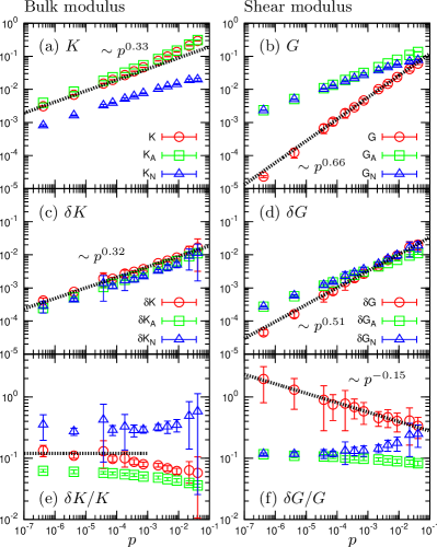
Figure 1: (Color online) Elastic modulus dependence on packing pressure, $p$. The average (global) total, affine ($A$), and non-affine ($N$) values $X,X_{A},X_{N}$, and corresponding standard deviations $\delta X$ of the probability distribution $P(X^{m})$, for $X^{m}=K^{m}$ (left panels) and $G^{m}$ (right panels). The CG domain is cubic of linear size $w\simeq 3$. Lines are power-law scalings with $p$. The presented data were obtained using the $T=0$ protocol with $N=1,000$ and averaging over $10$ different realizations at each value of $p$.

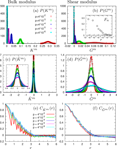
Figure 2: (Color online) Probability distributions of (a) $K^{m}$ and (b) $G^{m}$, and their relative fluctuations, (c) $\hat{K}^{m}=(K^{m}-K)/K$ and (d) $\hat{G}^{m}=(G^{m}-G)/G$, for the range of $p$ indicated in the legend of panel (a). Spatial correlation functions $C_{\hat{X}^{m}}(r)$ (defined in main text) for (e) $\hat{K}^{m}$ and (f) $\hat{G}^{m}$. The inset to (b) shows the fraction of negative $G^{m}$ regions, $F_{n}=\int_{G^{m}<0}P(G^{m})dG^{m}$, as a function of $p$. A close-up of $P(\hat{K}^{m})$ is shown in the inset to (c). In (a)-(d), solid lines indicate Gaussians. In (e),(f), vertical lines indicate the CG length, $r=w_{\alpha}=w\simeq 3$. Data were obtained using the $T=0$ protocol for $N=1,000$.

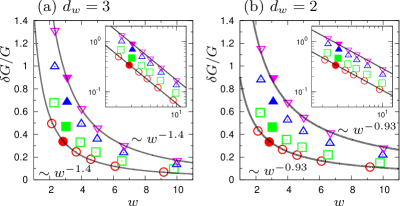
Figure 3: (Color online) Dependence of $\delta G/G$ on the CG length $w$ for (a) $d_{w}=3$ and (b) $d_{w}=2$, as discussed in main text. Same symbols used as key in Fig. 2(a). Closed symbols are data using $w_{\alpha}=w\simeq 3$, i.e. same data as shown in Fig. 1(f). Lines are power-law scalings, (a) $\delta G/G\sim w^{-1.4}$ and (b) $\sim w^{-0.93}$, consistent with $\delta G/G\sim w^{-d_{w}/2}$. Insets: same plots on log-log scales. For $w<6$ data were obtained by the $T=0$ protocol with $N=1,000$, and for $w>6$ the $T>0$ protocol with $N=10,000$.

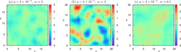
Figure 4: (Color online) Spatial maps of local shear modulus fluctuations, $\hat{G}^{m}=(G^{m}-G)/G$, within a fixed $x$-$y$ layer, for $d_{w}=3$. (a) Large pressure $p=4\times 10^{-2}$ and small CG length $w\simeq 3$, (b) small $p=4\times 10^{-5}$ and small $w\simeq 3$, and (c) small $p=4\times 10^{-5}$ and large $w\simeq 6.5$. Data were obtained using the $T>0$ protocol with $N=10,000$. Additional snapshots shown in Supplemental Material sup .

We now turn to a more explicit view of the spatial distributions of $K^{m}$ and $G^{m}$. Figure 2 presents the probability distributions $P({K}^{m})$ in (a) and $P({G}^{m})$ in (b). We find that all the $P(X^{m})$ are well-characterized as Gaussian over the entire pressure range, even down to the jamming point jno (c). But notice that although all the $K^{m}>0$, $G^{m}$ can contain negative values. The fraction of these negative shear modulus zones, $F_{n}=\int_{G^{m}<0}P(G^{m})dG^{m}$, is shown in the inset to Fig. 2(b). $F_{n}$ grows as $p\to 0$, suggesting that there is a $1:1$ ratio of stable and unstable regions jno (d) as the system becomes fragile Cates et al. (1998). Note the fact that our data appear to level off at the lowest pressure is likely a system size effect Goodrich et al. (2012). In Fig. 2(c), (d), we plot $P(\hat{K}^{m})$ and $P(\hat{G}^{m})$ of the fluctuations relative to global value, $\hat{X}^{m}=(X^{m}-X)/X$. $P(\hat{G}^{m})$ broadens significantly as $p$ decreases, which is quantitatively demonstrated by $\delta G/G$ in Fig. 1(f) jno (e), whereas variations in $P(\hat{K}^{m})$ are rather small and insensitive to $p$, consistent with $\delta K/K$ in Fig. 1(e).

In an effort to directly detect a correlation length associated with these fluctuations, the bottom panels of Fig. 2(e), (f) show the fluctuation spatial correlation function, $C_{\hat{X}^{m}}(r)={\left<\hat{X}^{m}(\mbox{\boldmath$r$})\hat{X}^{m}(\mbox{\boldmath$0$})\right>}/{\left<\hat{X}^{m}(\mbox{\boldmath$0$})\hat{X}^{m}(\mbox{\boldmath$0$})\right>}$, where we explicitly represent $\hat{X}^{m}$ as a function of position $r$, and $\left<\right>$ denotes a spatial average. Both the $C_{\hat{X}^{m}}(r)$ decay with the CG length $r=w\simeq 3$ jno (f), indicating that $K^{m}$ and $G^{m}$ fluctuate randomly in space without any apparent correlation, which persists all the way down to the transition point. Thermal glasses Yoshimoto et al. (2004); Mizuno et al. (2013a); Tsamados et al. (2009); Mizuno et al. (2013b, 2014) and disordered crystals Mizuno et al. (2013b, 2014) similarly exhibit random distributions in their local moduli that are Gaussian.

An alternative view to determining a possible characteristic length is through the dependence of fluctuations, $\delta X/X$, on the size of CG domain, $w_{x}\times w_{y}\times w_{z}$. We considered three different ways to change the CG domain: Vary, (i) $w_{x},w_{y},w_{z}$ equally, so that $w_{x}=w_{y}=w_{z}=w$, (ii) $w_{x},w_{y}$ as $w_{x}=w_{y}=w$, keeping fixed $w_{z}\simeq 3$, (iii) only $w_{x}$ as $w_{x}=w$, keeping fixed $w_{y}=w_{z}\simeq 3$. In (i), the CG domain is always cubic, whereas it becomes rectangular parallelepiped in (ii), (iii). We define the dimension $d_{w}$ of CG domain; $d_{w}=3,\ 2,\ 1$ for (i), (ii), (iii). As we have seen so far, $X^{m}$ is a random variable, following a Gaussian $P(X^{m})$. Thus, within the framework of a sum of random variables jno (g), we obtain the scaling law with respect to CG length $w$:

$${\delta X}/{X}\sim w^{-d_{w}/2}.$$ (4)

Figure 3 shows the $w$-dependence of $\delta G/G$ at several different $p$, for $d_{w}=3$ in (a) and $d_{w}=2$ in (b) (see sup for $d_{w}=1$). For all pressures, $\delta G/G\sim w^{-1.4}$, $\sim w^{-0.93}$, $\sim w^{-0.47}$ for $d_{w}=3$, $2$, $1$, respectively, which all confirm Eq. (4). We obtained the same result in $\delta K/K$. The same power-law dependence on $w$ has been reported for glasses, with exponent $1$ in $d_{w}=2$ Tsamados et al. (2009) and $1.5$ in $d_{w}=3$ Mizuno et al. (2013a).

Combining the scaling results for $\delta G/G$ (Eqs. (3) and (4)), expresses that relative fluctuations in shear modulus are suppressed over sufficiently large $w$. This supports the existence of a characteristic length, $\xi_{G}$, above which fluctuations become negligible. Specifically, we define $\xi_{G}$ as $w$ at which we see a fixed value, $\alpha_{0}$, of $\delta G/G$ for all $p$ or $\Delta\phi$, i.e. we determine $\xi_{G}$ as $\delta G/G=\alpha_{0}(w/\xi_{G})^{-d_{w}/2}$, which gives jno (h, i)

$$\xi_{G}\sim\Delta\phi^{-\nu_{\xi}},\quad\nu_{\xi}=\nu_{G}/(d_{w}/2).$$ (5)

The idea of the length $\xi_{G}$ associated with growing $\delta G/G$ is best visualized in Fig. 4, which shows the local fluctuations of shear modulus (for $d_{w}=3$) as follows: Panels (a) and (b) of Fig. 4 compare modulus maps of $\hat{G}^{m}=(G^{m}-G)/G$ for a slice through two packings at two different $p$, at the same $w\ \simeq 3$. In relation to Fig. 3(a) ($d_{w}=3$), these two points lie at different values of $\delta G/G$ along a vertical line at $w\simeq 3$, that intersect the respective $p$ curves. At this value of $w$, the two systems appear very different. Far from $\phi_{c}$, Fig. 4(a) ($p=4\times 10^{-2}$), the system appears quite uniform, and fluctuations are suppressed. Whereas, close to $\phi_{c}$, Fig. 4(b) ($p=4\times 10^{-5}$), we observe large-scale, spatial fluctuations. For the system closer to $\phi_{c}$ (small $p$), fluctuations become suppressed at the larger $w=6.5$ (Fig. 4(c)), so that the map resembles more compressed system at the smaller value of $w$. This corresponds to drawing a horizontal line across Fig. 3(a) at the same value of $\delta G/G$ connecting the two curves at different $p$.

In conclusion, we found that the differeces between bulk and shear moduli fluctuations, as the jamming point is approached, are caused by the non-affine components. Relative fluctuations in the bulk modulus become insensitive to packing pressure as $\Delta\phi\rightarrow 0$. Whereas, shear modulus fluctuations increase as, $\delta G/G\sim\Delta\phi^{-\nu_{G}}$, which leads to the identification of a lengthscale, $\xi_{G}\sim\Delta\phi^{-\nu_{\xi}}$. For CG dimension, $d_{w}=3$, $\nu_{\xi}\approx 0.16$, a value distinct from any previous study Ellenbroek et al. (2006); Lerner et al. (2014); Karimi and Maloney (2015); Vitelli et al. (2010); Goodrich et al. (2013); Schoenholz et al. (2013); Ikeda et al. (2013). $\xi_{G}$ corresponds to a scale above which the elastic properties coincide with those of the bulk system, while below, the local mechanical properties deviate from macroscopic behavior. It has been proposed that a continuum elastic description breaks down below a scale, $\ell_{c}\sim\Delta\phi^{-1/4}$ in two dimensions Lerner et al. (2014), consistent with our $\xi_{G}$ for $d_{w}=2$, and can derive from the transverse component of elastic response Karimi and Maloney (2015), which are controlled by shear modulus fluctuations.

At the same time, however, we also found that the local elastic moduli randomly fluctuate without any apparent correlations. This feature seems to be general for a wide class of disordered materials, thus further promoting the idea that granular-like particle systems present a model state for examining mechanical properties of disordered materials. Curiously, the randomness in local moduli persists down to the transition point and is different from the distribution of contact forces, which becomes more exponential closer to $\phi_{c}$ Makse et al. (2000) and is therefore more suggestive of spatial correlations. Such random fluctuations in the moduli may come from the coarse-graining procedure and/or the random distribution of particle contacts, which is a topic for future investigation.