Aggregation by Provenance Types: A Technique for Summarising Provenance Graphs

Abstract

As users become confronted with a deluge of provenance data, dedicated techniques are required to make sense of this kind of information. We present Aggregation by Provenance Types, a provenance graph analysis that is capable of generating provenance graph summaries. It proceeds by converting provenance paths up to some length $k$ to attributes, referred to as provenance types, and by grouping nodes that have the same provenance types. The summary also includes numeric values representing the frequency of nodes and edges in the original graph. A quantitative evaluation and a complexity analysis show that this technique is tractable; with small values of $k$, it can produce useful summaries and can help detect outliers. We illustrate how the generated summaries can further be used for conformance checking and visualization.

1 Introduction

In the world of art, the notion of provenance is well understood. A piece of art sold in an auction is typically accompanied by a paper trail, documenting the chain of ownership of this artifact, from its creation by the artist to the auction. This documentation is referred to as the provenance of the artifact. Provenance allows experts to ascertain the authenticity of the artifact, which in turn influences its price. This paper is concerned with an electronic representation of provenance for data, documents, and in general things in the world.

Provenance is a record that describes how entities, activities, and agents have influenced a piece of data [23]. It can help users make trust judgements about data. prov is a set of W3C specifications [13] aiming to facilitate the representation and exchange of provenance on the Web. prov is a graph-based data model that is domain-agnostic and has been applied to a wide range of applications, including climate assessment, legal notices, crowd sourcing [15], and disaster response [9].

As prov gets broader adoption, increasing numbers of applications continuously generate provenance, leaving users with a “provenance data deluge” making it challenging for them to make sense of this information. Users are confronted to questions such as Q1: “What is the essence of the provenance presented to me?”, Q2: “Is today’s behaviour conformant to yesterday’s provenance" or Q3: “Are there anomalies or outliers in an execution that deserve further investigation?". Such questions become very quickly untractable as provenance traces grow, and their graphical representation fills entire screens.

Network analysis techniques can effectively process graphs; for instance, graph clustering seems a particularly relevant approach to address question Q1 [26]. However, these techniques usually rely on statistical measures [27] and result in representations where the meaning of provenance is lost.

Research in semi-structured databases [4, 25, 11] offers partial answers to our problem. Notions of graph schemas that can be extracted from graph data [25, 11] can be used to summarise such data, offering an explanation about their structure, or helping formulate SPARQL queries [5, 16]. Unfortunately, no approach is provenance-specific and capable of generating a summary that exposes the meaning of provenance relations. However, the concept of conformance to a schema [4] is particularly relevant to addressing question Q2.

Visualization techniques use node size and line thickness for quantitative comparisons and for conveying a sense of salience of nodes and edges [29]. While our focus is not on visualization, the idea of a weight to describe the importance of an aspect is relevant. This is a critical element that can help identify outliers in large data sets [3], and can be the basis of a solution to Question Q3.

Meanwhile, there is a general trend of developing reusable and composable provenance graph transformations, for many purposes, including normalization [6], obfuscation [21]. Our aim is to define a summarization functionality as a transformation, which can be used further, e.g., for visualization or conformance check. Specifically, we seek to generate a summary that has the following key characteristics:

1. A summary needs to preserve the meaning of provenance. Humans tend to aggregate historically distant entities, regarding them as “similarly blurred in the past”. But also a summary needs to distinguish entities that were obtained by distinct historical paths, since such paths may affect their trustworthiness.

2. A summary needs to contain numerical information about the frequency of elements of provenance graphs to enable outliers detection.

Thus, we decided that “provenance paths”, i.e. successions of provenance relations, should play a central role in our approach. For instance, an entity derived from an entity attributed to an agent is a path of length 2. The intuition of our solution is to regard a provenance path of length $k$ leading to a node as a “provenance type” for that node. Then, we construct a summary by aggregating all nodes that have the same provenance types, and likewise for edges, and by counting their occurrences. The method, named Aggregation by Provenance Types, $\mbox{\sc apt}(k$), is parametric in the maximum path length. Specifically, the contributions of this paper are the following.

1. A provenance graph analysis and transformation apt that creates a summary of a provenance graph; this summary itself is built using the same provenance vocabulary, but should be seen as a provenance graph “schema” decorated with frequency information.

2. A complexity analysis of this algorithm, followed by a quantitative evaluations of the technique, showing its tractability, and by a discussion further showing its ability to expose salient properties of provenance graphs.

3. An illustration of how apt can be used in two applications such as visualization and conformance checking.

The rest of this paper is structured as follows. First, we identify the requirements that a summarisation technique is expected to meet (Section 2). Then, we define the notion of provenance type and the technique of “aggregation by provenance types” (Section 3). It is followed by a complexity analysis of the approach (Section 4). We then illustrate two different applications of apt (Section 5). This is followed by a quantitative evaluation of the approach (Section 6) and a discussion (Section 7). Related work appears in Section 8 and the paper finishes with concluding remarks (Section 9).

2 User Requirements for Summarisation

The three questions of Section 1 form key user requirements that a provenance summarisation technique should satisfy. The first requirement is inspired by Q1 of Section 1 and some well-known requirements captured by the W3C Incubator group (see http://www.w3.org/2005/Incubator/prov/wiki/User_Requirements#Use) identifying the need to make provenance information understandable. The following two requirements reflect directly Questions 2 and 3 of Section 1.

Requirement 1 (Essence of Provenance)

A provenance summary should capture the essence of the provenance graph that it summarises.

Requirement 2 (Conformance)

It should be possible to decide whether a provenance graph is compatible, or conformant, with a provenance summary.

Requirement 3 (Outliers)

It should be possible to detect anomalies or outliers in a provenance summary.

We satisfy Requirement 1 by adopting the same language for summaries as for provenance graphs. As we aggregate nodes and edges, we keep a count of the nodes and edges that were collapsed; such numerical values can help a user or system detect outliers. Finally, given that summaries are based on the same language as provenance graphs, it becomes easy to check whether one is compatible with the other; for instance, techniques such as simulations from process algebra [14] can be applied to this problem [4].

Every day processes illustrate that we focus on more or less recent past, according to how discriminating we want to be. For instance, a selective graduate school may admit PhD applicants who have a first-class degree from a reputable University. A more selective graduate school will also require good transcripts from secondary school, or extra-curricula activity related to the subject. However, older information, such as performance in primary school, is generally not used as discriminator. In manufacturing or food production, the country of origin is deemed to be the place of last substantial change. However, to avoid misleading food labels, the origin of the primary ingredient should also be considered. These two examples show that individuals are distinguished according to their past — more or less recent. Thus, the distance in the past can abstracted by a parameter $k$, which we use in our aggregation method.

3 Aggregation by Provenance Types

The purpose of this section is to define Aggregation by Provenance Types, abbreviated by apt. To do so, we first introduce the notion of provenance type.

A provenance type is defined as a category of things that have common characteristics from a provenance perspective. Provenance types are parameterised by an integer indicating the length of provenance paths used to characterise things. A level-0 provenance type is one of the core type predefined in prov: prov:Entity, prov:Activity, and prov:Agent, or any user-defined type. A level-$k+1$ provenance type is an expression describing the category of things one prov-relation away from things that have a level-$k$ provenance type.

For instance, in :a0 prov:used :e1, if :e1 is assigned level-$k$ provenance type $\tau_{k}$, then :a0 is assigned level-$k+1$ provenance type $used(\tau_{k})$, meaning that :a0 belongs to the category of things that used something of type $\tau_{k}$. Likewise, in :e2 prov:wasDerivedFrom :e1, if :e1 is assigned level-$k$ provenance type $\tau_{k}$, then :e2 is assigned level-$k+1$ provenance type $\mathit{wdf}(\tau_{k})$, meaning that :e2 belongs to the category of things that were derived from something of type $\tau_{k}$.

Definition 1

A provenance type of level $k$, noted $\tau_{k}$, is defined as follows.

$$\begin{array}[]{rcl}\tau_{0}&::=&Entity\ \ |\ \ Activity\ \ |\ \ Agent\ \ |\ \ \mbox{user-defined type}\\ \tau_{k+1}&::=&label(\tau_{k})\end{array}$$

where ‘$label$’ is a prov property label defined as follows.

$$\begin{array}[]{|l|l||l|l|}\hline\cr\mbox{Label}&\mbox{{\sc prov} property}&\mbox{Label}&\mbox{{\sc prov} property}\\ \hline\cr\hline\cr used&\mbox{\href http://www.w3.org/ns/prov#used}&wsb&\mbox{\href http://www.w3.org/ns/prov#wasStartedBy}\\ wgb&\mbox{\href http://www.w3.org/ns/prov#wasGeneratedBy}&web&\mbox{\href http://www.w3.org/ns/prov#wasEndedBy}\\ \mathit{wdf}&\mbox{\href http://www.w3.org/ns/prov#wasDerivedFrom}&\mathit{wifb}&\mbox{\href http://www.w3.org/ns/prov#wasInformedBy}\\ waw&\mbox{\href http://www.w3.org/ns/prov#wasAssociatedWith}&mem&\mbox{\href http://www.w3.org/ns/prov#hadMember}\\ wat&\mbox{\href http://www.w3.org/ns/prov#wasAttributedTo}&spec&\mbox{\href http://www.w3.org/ns/prov#specializationOf}\\ aobo&\mbox{\href http://www.w3.org/ns/prov#actedOnBehalfOf}&alt&\mbox{\href http://www.w3.org/ns/prov#alternate}\\ wib&\mbox{\href http://www.w3.org/ns/prov#wasInvalidatedBy}&&\\ \hline\cr\end{array}$$

Note that Definition 1 lists forward properties of prov only, but could also consider prov inverse properties [19]. Provenance types with forward properties refer to what led to that node (i.e., the past of the node), whereas provenance types with inverse properties refer to what happened to that node (i.e., its future).

We introduce the properties ann:pType0, ann:pType1, …that associate a resource with its provenance types of level 0, 1, …, respectively. A given resource may be the subject of multiple provenance types properties. Figure 1 displays a template of SPARQL query to compute provenance types.

PREFIX prov: <http://www.w3.org/ns/prov#>
PREFIX ann: <http://provenance.ecs.soton.ac.uk/annotate/ns/#>

CONSTRUCT {  ?y ?pType_kp1 ?provenanceType. }
WHERE {
   {
      ?y prov:wasDerivedFrom ?x.
      ?x ?pType_k ?t.
      BIND (CONCAT("wdf(",?t,")") AS ?provenanceType)
   }
   UNION
   {
      ?y prov:used ?x.
      ?x ?pType_k ?t.
      BIND (CONCAT("used(",?t,")") AS ?provenanceType)
   }
   // .... and similarly for other prov relations
}

Figure 1: Pattern of SPARQL Query to Compute Provenance Types of Level $k+1$. Provenance types are expressed as a string encoding of Definition 1.

PREFIX prov: <http://www.w3.org/ns/prov#>
PREFIX ann: <http://provenance.ecs.soton.ac.uk/annotate/ns/#>

CONSTRUCT {  ?x ann:pType0 ?provenanceType. }
WHERE {
   {
     ?x a prov:Entity.
     ?x rdf:type ?b.
     BIND (CONCAT("",strafter(STR(?b),"#")) AS ?provenanceType)Ψ
   }
   UNION
   // and similarly for prov:Agent and prov:Activity
}

Figure 2: Pattern of SPARQL Query to Compute Provenance Types of Level 0

In the query template, variables ?pType_k and ?pType_kp1 have to be instantiated to the properties reflecting the value $k$ of interest: for instance, ann:pType3 and ann:pType4, respectively, for $k=3$. A provenance type for level $k=0$ is computed by the SPARQL query of Figure 2, which assigns ann:pType0 to each resource of type prov:Entity, prov:Activity, or prov:Agent. We assume that RDFS-reasoning has inferred prov core types.

The graph transformation Level-k Aggregation by Provenance Types, written $\mbox{\sc apt}(k)$, constructs a provenance summary by grouping all the nodes that have the same provenance types $\tau_{i}$ for any $i$ such that $0\leq i\leq k$, and then merging all edges, as specified in Definitions 2 and 3.

Definition 2 (Node Aggregation)

Given a prov document $D$, node aggregation for a value $k$ is a set of types $T=\{t_{0},t_{1},...,\}$ and a type assignment $f:Node\rightarrow T$, such that the following hold:

• If $f(x)=f(y)$ then $\phi(x,k)=\phi(y,k)$, for any node $x,y\in D$.

• If $f(x)\not=f(y)$ then $\phi(x,k)\not=\phi(y,k)$, for any node $x,y\in D$.

where $\phi(x,k)=\{\tau_{i}|\tau_{i}\ \mbox{ is a provenance type of level $i$ for $x$, such that $0\leq i\leq k$}\}$.

Further, $\mbox{\it Nodes}:T\rightarrow N$, the weight of each summary type, is defined as $\mbox{\it Nodes}(t)=|\ \{x\ |\ f(x)=t\}\ |$.

Definition 3 (Edge Aggregation)

Let $D$ be a prov document. Let $T$ be a set of types $\{t_{0},t_{1},...,\}$ and $f:Node\rightarrow T$ be a type assignment obtained by node aggregation for some $k$. Let $\psi(t_{0},t_{1},lab)$ be a set of edges $\{x\rightarrow^{lab}y\in D\ |\ f(x)=t_{0}\mbox{ and }f(y)=t_{1}\}$. Edge aggregation results in a weighted set of labeled edges, defined as follows: $Edges:T\times T\times Label\rightarrow N$, with $Edges(t_{0},t_{1},lab)=|\psi(t_{0},t_{1},lab)|\mbox{ for any }t_{0},$ $t_{1},lab$.

From Definitions 2 and 3, we can now define apt.

Definition 4 (Aggregation by Provenance Types)

Let $D$ be a prov document and level $k\geq 0$ be a natural number. Aggregation by Provenance Type, $\mbox{\sc apt}(k)(D)$ is a summary $S$ such that:

• vertices of $S$ are the set $T=\{t_{0},t_{1},...,\}$ obtained by node aggregation for $k$, with type assignment $f$ mapping nodes of $D$ to $S$, and weight Nodes.

• a weighted set of labeled edges $Edges$ obtained by edge aggregation for type assignment $f$.

As type labels ($t_{0},\ldots$) are generated by apt, summaries that only differ by type labels are regarded as equivalent. Hence, we consider summary equivalence up to type naming.

Provenance summaries are also graphs whose nodes and edges are expressed according to prov. However, summaries in general are not valid [6] provenance graphs: indeed, collapsing nodes that have the same provenance types may introduce cyclic derivations or specializations, which are invalid [6]. For instance, if a summary contains a triple :T prov:wasDerivedFrom :T, it should be understood as: an entity of type :T was derived from another entity of type :T.

Inspired by the notion of conformance of a graph to a schema [4], we can define a notion of conformance to a summary. (We assume that some nodes have been identified as ‘‘root’’, from which all other nodes can be reached.)

Definition 5 (Conformance to a Summary)

A provenance graph instance $G$ conforms to a provenance graph summary $S$, in notation $G\preceq S$, if there exists a simulation from $G$ to $S$, i.e. a binary relation $\preceq$ from the nodes of $G$ to those of $S$ satisfying (1) the root nodes of $G$ and $S$ are in the relation $\preceq$, (2) whenever $u\preceq u^{\prime}$ and $u\rightarrow^{a}v$ is an edge labeled $a$ in $G$, then there exists some edge between $u^{\prime}$ and $v^{\prime}$ for label $a$ in $S$, i.e. $Edges(u^{\prime},v^{\prime},a)>0$, such that $v\preceq v^{\prime}$.

Lemma 1

A provenance graph is conformant to any summary produced by $\mbox{\sc apt}(k)$ for any $k$.

Proof is straightforward since the type assignment $f$ of Definition 2 provides a simulation from the graph to its summary.

4 Complexity Analysis

Following Definition 1, the length of $\tau_{k+1}$ is bounded by the length of $\tau_{k}$ plus a constant. Thus, if $C_{I}$ is the maximum number of incoming edges per node, $N$ the number of nodes, and $c$ a constant, then the cost of computing all annotations for all nodes is:

$$cost(all\ \tau_{k})<N(C_{I})^{k}+c$$

This means that computing provenance types is linear in the size of the graph, but exponential in the analysis’ level-$k$. In the presence of graphs with cycles (even valid graphs [6]) the size of type information may become exponentially large with $k$. Figure 3 illustrates how provenance types grow as $C_{I}$ is $2>1$, while the summary remains homomorphic to the original graph.

:e1 a prov:Entity.
:e2 a prov:Entity.
:a a prov:Activity.
:ag a prov:Agent.
:e1 prov:wasGeneratedBy :a.
:e2 prov:wasGeneratedBy :a.
:a prov:used :e1.
:a prov:used :e2.
:e1 prov:wasAttributedTo :ag.
:e2 prov:wasDerivedFrom :e1.

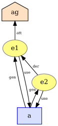
$$\begin{array}[b]{l}\mbox{provenance types for $a$}\\ \tau_{0}=Activity\\ \tau_{1}=\{used(Entity)\}\\ \tau_{2}=\{used(wat(Agent)),\\ \ \ \ \ \ \ \ \ used(\mathit{wdf}(Entity))\}\\ \ \ \ \ \ \ \ \ used(wgb(Activity))\}\\ \ldots\\ \tau_{4}=\{\mathit{wdf}(wgb(used(wat(Agent)))),\\ \ \ \ \ \ \ \ \ \mathit{wdf}(wgb(used(\mathit{wdf}(Entity)))),\\ \ \ \ \ \ \ \ \ \mathit{wdf}(wgb(used(wgb(Activity)))),\\ \ \ \ \ \ \ \ \ wgb(used(\mathit{wdf}(wat(Agent)))),\\ \ \ \ \ \ \ \ \ wgb(used(\mathit{wdf}(wgb(Activity)))),\\ \ \ \ \ \ \ \ \ wgb(used(wgb(used(Entity))))\}\\ \ldots\end{array}$$

Figure 3: A Valid Provenance Graph with a Cycle and its Provenance Types

Note that this kind of complexity is typical of database graph schema techniques (see Section 8). Furthermore, while prov allows for some valid graphs to be cyclic, this case is not so frequent. In addition, in Section 6, we show that apt complexity is practical. First, for a given level $k$, apt is linear in the size of the input graph. Second, summaries produced for $k=1$ and $k=2$ are shown to be very usable. Third, we demonstrate that the size of the summary saturates when $k$ is greater than the longest chain of directed edges in the graph (see Hypothesis 2).

In our proof of concept implementation, computation of provenance types uses the SPARQL queries of Figures 1 and 2. Generation of summaries and SVG representation rely on ProvToolbox (http://lucmoreau.github.io/ProvToolbox/). Ontology generation uses the OWL-API.

5 Applications of APT --- Illustration

In this section, we provide two different applications of apt: interactive visualization and conformance check. We discuss them in turn.

5.1 Visualization for Exploring Provenance

Visualization tools for interactively exploring provenance could leverage summaries. While designing and implementing a summary-based visualization tool is beyond the scope of this paper, one can outline the appearance of a summary, and the modes of interaction that it would support in a visualization tool.

Figure 7 (right) illustrates how a a summary be visualized. There, the thickness of edges is determined by the relative value of their weight as computed in the summary. In a real implementation, the size of nodes would also be indicative of their respective frequencies.

As far as a visualization tool interface is concerned, we envisage two adjacent windows: on the left-hand side, a summary representation, and on the right-hand side, a graph instance. Selection of nodes/edges in the summary would automatically highlight corresponding nodes/edges in instance.

5.2 Conformance Check

We revisit Requirement 2. A provenance-enabled application generates a provenance trace, out of which a summary is generated by apt. The next day, the application continues to run, producing provenance again. An expert user may wonder whether the behaviour on the second say is conformant with the application’s behaviour on the first day. Conformance to a summary is defined in Definition 5.

To provide an illustration of conformance checking, we converted an apt-summary into an OWL2 ontology (discarding all the frequency information). In Figure 4, we find two defined classes ExecutionStep_5 and T_9 from the example of Figure 7 (right). The lines marked with $(\dagger)$ include basic types and definitions of edges, as displayed in Figure 7: for instance, T_9 is the source of a prov:wasGeneratedBy edge to either ExecutionStep_1 or ExecutionStep_5.

Conformance checking is performed under the closed world assumption: we consider here that we have complete knowledge. If a statement cannot be found in a provenance graph, it is considered not to be true. Hence, the defined classes are extended with the clauses $(\star)$ requiring the corresponding edges to be absent (maximum cardinality is zero). Similar clauses need to be generated for instances, to express that there is no other possible instances that can be asserted. Finally, all classes are defined to be mutually disjoint.

Hence, an instance of activity ExecutionStep_5 is expected to have used a Building834.1_2 and a Route2324.0_13, and be associated with User_6. The class ExecutionStep_5 is distinct from ExecutionStep514_12 which has no usage, but a similar association with User_6.

$${ExecutionStep\_5} \equiv \exists~{}used~{}Building834.1\_2\ \ (\dagger)$$

$$\sqcap~{}\exists~{}used~{}Route2324.0\_13~{}\ \ (\dagger)$$

$$\sqcap~{}\exists~{}wasAssociatedWith~{}User\_6\ \ (\dagger)$$

$$\sqcap~{}\leq~{}0~{}used\lnot(Building834.1\_2~{}\sqcup~{}Route2324.0\_13)\ \ (\star)$$

$$\sqcap~{}\leq~{}0~{}wasAssociatedWith~{}\lnot User\_6\ \ (\star)$$

$$T\_9 \equiv ~{}Vote\ \ (\dagger)$$

$$\sqcap~{}\exists~{}wasDerivedFrom~{}Building834.1\_2~{}\ \ (\dagger)$$

$$\sqcap~{}\exists~{}wasGeneratedBy~{}(ExecutionStep\_1~{}\sqcup~{}ExecutionStep\_5)\ \ (\dagger)$$

$$\sqcap~{}\leq~{}0~{}wasDerivedFrom~{}\lnot(Building834.1\_2)\ \ (\star)$$

$$\sqcap~{}\leq~{}0~{}wasGeneratedBy~{}\lnot(ExecutionStep\_1~{}\sqcup~{}ExecutionStep\_5)\ \ (\star)$$

Figure 4: OWL2 Definition for ${ExecutionStep\_5}$ and $T_{9}$ from Figure 7 (right)

6 Evaluation

In this section, we develop several hypotheses that we validate by applying apt to a set of provenance graphs and examining the results. For the purpose of evaluation, we consider provenance graphs generated by the following applications.

1. Atomic Orchid (ato) [?] is a real-time location-based serious game to explore coordination and agile teaming in disaster response scenarios [9]. Provenance in AtomicOrchid includes location and activities of participants, and orders issued by the headquarter.

2. CollabMap (col) [?] is an application that crowd-sources evacuation routes in a geographical area (with a view of simulating evacuations under various conditions) [15]. CollabMap provenance describes how all artifacts, i.e., building, routes, route sets, and votes, have been created.

3. Patina of Notes (pon) [?] is an application for collecting notes about archaeological artifacts, with a view to build, possibly multiple, interpretations of these artifacts [17]. The provenance includes the notes, their structures, and how they evolve over time.

4. The Provenance Challenge 1 (pc1) [?] workflow is representative of FMRI applications building brain atlases. It was the basis of the provenance challenge series and early provenance inter-operability efforts [22].

5. The PROV Primer (pri) [?] describes the activities around the editing of a document [10].

6. Linear Derivation (lin) [?] is a synthetic provenance graph exhibiting a linear sequence of successive derivations.

The apt graph transformation outputs a summary. Our first investigation, captured by Hypothesis 1, is concerned with the size of apt’s output. Intuitively, in the worst case, when no node of the original graph can be aggregated by apt, the output has the same size as the input. In the best case, all nodes can be merged in a single one; compression is then maximum.

Hypothesis 1 (Compression)

Given a provenance graph $G$, apt results in a summary whose number of nodes is smaller than or equal to the number of nodes in the original graph $G$.

Method We apply apt to the selected set of provenance graphs, and compare the number of types produced by apt with the number of input nodes, for types entity, activity, and agent. To be able to compare the relative performance of apt on the different graphs and different types, we plot the ratio ‘‘number of types : number of input nodes’’. Figure 5 plots such a ratio for $\mbox{\sc apt}(2)$.

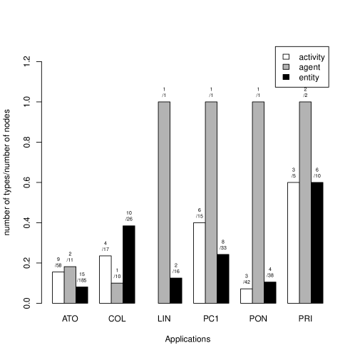
Figure 5: Ratio ‘‘number of output types : number of input nodes’’ for $\mbox{\sc apt}(2)$. The smaller the more compressed. Above each bar, we find the ratio $x/y$, where $x$ denotes the absolute number of output types, whereas $y$ denotes the absolute number of input nodes. Plot can also be found online.

Analysis We see a significant reduction in size (compression ratio between 3 and 10) for applications ato, col, lin, pc1, pon, except for agents (which happen to be in small number for some graphs and cannot be aggregated further). The exception is pri, which describes a fairly unstructured series of human activities related to editing a document: very few nodes can be aggregated together, resulting in a small compression rate.$\Box$

Figure 5 plots one point in the space of possible outputs of apt. As apt level increases, the analysis is better able to discriminate nodes that have a different history: thus, the number of types also increases, until it saturates, as expressed by Hypothesis 2. This hypothesis relies on a graph metrics, Maximum Finite Distance, MFD [8], which is a provenance-specific variant of graph diameter.

Hypothesis 2 (Monotonic)

The number of output types of $\mbox{\sc apt}(k)$ is a monotonically increasing function of $k$ that plateaus once $k$ reaches the graph’s Maximum Finite Distance (MFD).

Method We apply apt to the selected set of provenance graphs, and compare the total number of types produced by $\mbox{\sc apt}(k)$ with the total number of input nodes. Figure 6 plots the ratio ‘‘number of types : number of input nodes’’, for increasing values of $k$.

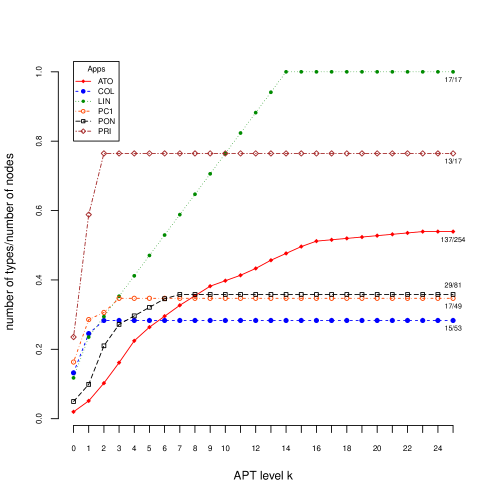
app	plateau for $k$	MFD [8]
ato	24	24
col	2	4
lin	14	15
pc1	4	6
pon	7	8
pri	2	4

Figure 6: Ratio ‘‘number of output types : number of input nodes’’ for $\mbox{\sc apt}(k)$, for increasing values of $k$. We also express the ratio $x/y$ when apt plateaus (where $x$ denotes the number of output types, whereas $y$ denotes the number of input nodes). Plot can also be found online.

Analysis For each application, $\mbox{\sc apt}(k)$ reaches a plateau for a given value of $k$. The table in Figure 6 records this value as well as the MFD measure of the corresponding graph, computed according to [8]. We see that the plateau is reached for a value of $k$ smaller than the graph’s MFD. Intuitively, this can be explained by the fact that no distinct provenance type can be propagated on chains longer than the Maximum Finite Distance.

In some cases, such as lin, the types identified by apt have a direct connection with the nodes of the input graph. In such circumstances, with a value of $k$ that is large enough, apt is capable of distinguishing all nodes, and therefore does not aggregate any. In other cases, such as pc1, no level of apt is able to distinguish some input nodes. Indeed, the workflow operates over a collection of images (3 in this specific instance). Given that their treatment is uniform, no apt analysis can distinguish them, unless they are explicitly assigned some distinct base types.$\Box$

The reason why apt is capable of compressing the input graph (see Hypothesis 1) is that apt can represent repeated graph patterns in a more compact manner in the summary. Hypothesis 3 relates numeric values in the summary to the repeat of patterns in the original graph.

Hypothesis 3 (Repeated Patterns)

Types produced by $\mbox{\sc apt}(k)$ with occurrences $>k$ are likely to be members of graph patterns repeated more than $k$ times.

Method After applying apt to a provenance graph, we plot the number of nodes for each type identified by apt. The types with number of nodes $>k$ are candidate nodes of repeated patterns.

Analysis We note that apt itself does not detect patterns, but instead apt helps identify types that occur in repeated patterns. Due to space shortage, we focus on col only; the analysis could be performed on other graphs with a similar outcome. Figure 7 (left) illustrates a provenance summary produced by $\mbox{\sc apt}(1)$ on col, and the corresponding scatter plot (types vs node occurrences). Figure 7 (right) displays a provenance summary, in which the thickness of edges is proportional to the number of edges in the original graph instance. Figure 8 displays examples of repeated patterns. We see that there are 6 and 7 occurrences for types ExecutionStep_1, ExecutionStep_5 and T_9, respectively, in Figure 7 (left), whereas there are 6 and 10 occurrences for nodes of type T_4 and User_6, respectively.$\Box$

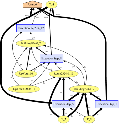
Figure 7: The scatter plot on the left-hand side displays the various types against the number of nodes for each types. The provenance summary on the right-hand side is obtained by application of $\mbox{\sc apt}(1)$ to col. The thicker the edge in the summary, the more edge instances between nodes with corresponding types. Left and right sides are available online here and here, respectively.

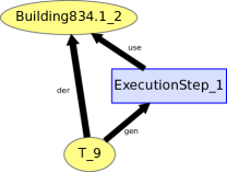
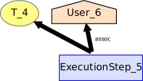
Figure 8: Example of Two Graph Patterns Occurring 6 Times in col

7 Discussion

The apt transformation results in a summary that includes nodes and edges frequencies. Figure 7 (right) illustrates this information in a simple graphical way. We believe that this information could be the basis of a provenance visualization tool, but developing such a tool would require substantial work beyond the scope of this paper. Instead, we had a discussion with the provenance expert behind the generation of col provenance, explaining apt and discussing some graphical illustrations, including the one in Figure 7 (right). This section summarises some highlights of the discussion, which was centered around the need to make provenance understandable (see Section 2).

apt output is helpful to derive a narrative from a provenance graph.

The bold edges are useful to express a narrative. ‘‘A building (Building834.0_7) is identified (ExecutionStep514_12), and voted upon (ExecutionStep_8); a route (Route2324.0_13) drawn and voted upon (ExecutionStep_5); and, a route set (Building834.1_2) defined and voted upon (ExecutionStep_1).’’ A visualization tool leveraging apt but also application types would be able to expose such a narrative in a compelling way. Thus, we conclude that apt provides solid foundations to address the introduction’s Question Q1, reflected in Requirement 1.

apt helps get a good insight in the way provenance is modelled.

As we were discussing the high-level narrative, our attention was drawn to an activity type (ExecutionStep_8) that results in a vote (UpVote_10) and a route (Route2324.0_13). Upon further investigation, it was discovered that this type encompasses two different kinds of activities (voting and drawing route, respectively) of the original provenance graph, but there was nothing to distinguish those activities since they have the same provenance type: namely, they they use a building and are associated with some user, according to some plan. Given that all the plans are aggregated as entities that do not have any ancestor, they all appear as a simple type (T_8). By distinguishing these types of plans, distinct activity types would be produced in place of ExecutionStep_8. Again, this discussion shows that apt helps address Requirement 1.

apt helps detect outliers.

Large edges in the provenance summary are indicative of repeated patterns (Hypothesis 3). Hence, occurrence of a thin edge within a repeated pattern is highlighting the presence of an unusual phenomenon. For instance, in Figure 7 (right), T_9 is suspiciously generated from ExecutionStep_5 with a thin edge. An investigation shows that this edge links a negative vote on a route set to a voting activity on a route: when a route is voted negatively, so is the route set it is contained in. Such phenomenon reveals something special that occurred at execution time, or alternatively it highlights some specific provenance modelling by the implementer. Hence, the weights included in apt summaries are a good mechanism to address the introduction’s Question Q3 (i.e. Requirement 3).

8 Related Work

There are relevant summarization techniques for general graphs, without focus on provenance. A DataGuide [11] consists of a dynamically-generated summary of a graph-structured database. A DataGuide for a source object $s$ is an object $d$ such that every label path of $s$ has exactly one data path instance in $d$ (conciseness), and every label path of $d$ is a label path of $s$ (accuracy). Incremental and non-incremantal algorithms are proposed to compute DataGuides, and their performance is studied. Also, techniques to optimise queries based on DataGuides are investigated. By construction DataGuides never include information that does not exist in the data. On the other hand, apt aggregate nodes that have the same provenance types, hereby potentially creating loops in the output: such loops could correspond to arbitrarily long paths in the original graph, a fundamental difference between the two approaches. Like apt, the construction of DataGuides has an exponential upper bound for cyclic graphs.

DataGuide’s ancestor, Representative Objects (RO) [24], is a form of summary that could be computed for a given graph database. One of its variants is a $k$-representative, which limits the summary to path expressions of length $k+1$. While the definition of RO($k$) is totally different from $\mbox{\sc apt}(k)$, both have in common the focus on paths of length $k$.

In subsequent work, Goldman and Widom [12] consider Approximate DataGuides, by lifting the accuracy constraint in the definition, and hereby not requiring every label path of $d$ to be a label path of $s$. They use a notion of set similarity based on the idea that two similar sets have a proportion of common elements above some threshold. Wang et al. [28] study a variant of Approximate DataGuides by maximising a utility function over a clustering of nodes. Related to our work is their taking into account of incoming and outgoing edge labels, though they focus on the size of label sets, rather than the labels themselves.

To optimise queries for the data web, Jarrar and Dikaiakos [16] introduce two notions of graph signature: the O-Signature (resp. I-Signature) is a summary of a graph such that nodes that have the same outgoing (resp. incoming) paths are grouped together. This notion is similar to a 1-Index [20], a computationally-efficient refinement over a language equivalence relation. The key differentiator is that paths of arbitrary length are considered in [16, 20], whereas apt limits itself to paths of length $k$.

Buneman et al. [4] define the notion of graph schema for a graph database. They further introduce the notion of a database conforming to a schema by a generalization of similarity. Intuitively, the set of label paths in a schema is a superset of label paths in the original graph.

Nestorov et al. [25] introduce the notion of approximate typing, and a measure in terms of defects (number of edges ignored or to be added to be able to check conformance). In that sense, the summary produced by apt is perfect. They also use a clustering technique to reduce the number of types, while keeping the number of defects minimum.

Observing that existing graph summarization methods are mostly statistical (e.g., degree distribution, distance, and clustering coefficients [26]), Tian et al. [27] propose two graph summarization techniques allowing resolutions of summaries to be better controlled. SNAP produces a summary graph by grouping nodes based on user-selected node attributes and relationships. SNAP produces a graph partitioning where all nodes in a grouping are homogeneous in terms of some user-selected attributes and relations; the partitioning is optimal in the sense that it contains a minimal number of nodes. A variant of this operation, $k$-SNAP require most nodes (as opposed to all) of a grouping to be involved in the selected relation, whereas they still all have the same attributes; users can select the number $k$ of groups in the summary. apt proceeds by converting provenance-related relations into provenance-type attributes. The grouping produced by apt is then equivalent to a SNAP operation over provenance-type attributes. The originality of apt is that it considers relation paths of lengh $k$, whereas SNAP focuses on direct relations.

Approximations, such as those described in [27, 25, 12, 28, 20], could be considered if the number of types produced by apt is too large. But all come with non-trivial computational overheads.

In the context of Business Activity Monitoring, process mining consists of extracting information about processes from transaction logs. Transactions logs typically are a strict subset of provenance information. The type of processes that can be extracted can be represented as Petri Nets [2].

Semantic substrates is a technique to group nodes into rectangular regions, and lay them within each region according to user-chose attributes. Node aggregation [3] is used to replace all the nodes in a grid cell with a single metanode. Likewise, PivotGraph [29] is a technique to visualize graph according to attributes selected by users. The techniques [3, 29] are complementary with apt: apt exposes provenance types as attributes, and these techniques empower the user to select which attributes to render, and offer original layouts. Koop et al. [18] propose a method to summarise graph collections: they use domain-specific comparison functions to collapse similar nodes and edges, with the aim §of producing more compact representations of such collections. An interesting study would be to focus on the suitability of all these visualization methods for provenance.

Means of abstracting provenance traces have been considered. ‘‘User views’’, defined as a partition of tasks in a workflow specification [7], provide the means to selectively identify what aspect of a provenance trace should be exposed to users. This approach differs from our work since our summaries are construted automatically without requiring an explicit workflow. Likewise, ‘‘abstract provenance graph’’ [30] are derived by static analysis of workflows. In addition, techniques are proposed to further summarise provenance graphs, based on time information and the structure of the worklow. Provenance graph abstraction by node grouping [21] is a technique by which a set of nodes in a prov-compliant provenance graph is replaced by a new abstract node with a view to obfuscate provenance; privacy policies are used to identify the nodes to group.

9 Concluding Remarks and Future Work

In this paper, we have presented a summarisation technique for provenance graphs. The approach consists of converting provenance paths, up to some length $k$ to node attributes (referred to as provenance types), and grouping nodes that have the same provenance types. The summary also contains numeric values representing the frequency of nodes and edges in the original graph.

A complexity analysis of the algorithm shows that it is linear in the size of the graph, and potentially exponential in the maximum path length $k$. Such a type of complexity is typical of related work. The positive side of our work is that our quantitative evaluation shows that the algorithm is perfectly tractable since useful summary graphs can be obtained with small values of $k$, and it was shown that for $k$ greater than the Maximum Finite Distance, the size of the summary saturates.

We also introduced a notion of conformance to a summary, which captures the idea that the summary includes all possible traversals that can be performed in a graph. We have illustrated how such conformance can be implemented by means of an OWL2 consistency check.

A qualitative discussion of the approach, based on a sample visualization based on the summarization, has shown that the approach has a good potential to detect anomalies and outliers. Overall, we have demonstrated that apt suitably addresses three use cases, formulated as questions in the introduction of the paper and expressed as requirements for summarisation.

With this paper, we have opened up a whole area of research in summarization techniques for provenance graphs, and their application to conformance checking and visualization. Our future work will seek to develop efficient algorithms for conformance checking. In addition, we will seek to investigate the incremental aspect of the approach: being able to adjust summaries and being able to check conformance incrementally as provenance graphs are extended. Furthemore, an issue that is particularly related is to find mechanisms to help users identify base types to construct provenance types. Finally, while the approach is developed in the context of provenance, it could have potential applications for any form of graphs; future research would have to clarify the intuition associated with so-called provenance types.

Acknowledgements

This work is funded in part by the EPSRC SOCIAM (EP/J017728/1) and ORCHID (EP/I011587/1) projects, the FP7 SmartSociety (600854) project, and the ESRC eBook (ES/K007246/1) project. Thanks to Trung Dong Huynh for feedback on a draft of this paper.

References

- [1]
- [2] Wil van der Aalst, Ton Weijters & Laura Maruster (2004): Workflow Mining: Discovering Process Models from Event Logs. IEEE Transactions on Knowledge and Data Engineering 16(9), pp. 1128--1142, 10.1109/TKDE.2004.47.
- [3] A. Aris & Ben Shneiderman (2008): A Node Aggregation Strategy to Reduce Complexity of Network Visualization using Semantic Substrates. Available at http://www.cs.umd.edu/localphp/hcil/tech-reports-search.php?number=2008-10.
- [4] Peter Buneman, Susan B. Davidson, Mary F. Fernandez & Dan Suciu (1997): Adding Structure to Unstructured Data. In: Proceedings of the 6th International Conference on Database Theory, ICDT ’97, Springer-Verlag, London, UK, UK, pp. 336--350, 10.1007/3-540-62222-5_55.
- [5] S. Campinas, T.E. Perry, D. Ceccarelli, R. Delbru & G. Tummarello (2012): Introducing RDF Graph Summary with Application to Assisted SPARQL Formulation. In: Database and Expert Systems Applications (DEXA’12), pp. 261--266, 10.1109/DEXA.2012.38.
- [6] James Cheney, Paolo Missier, Luc Moreau (eds.) & Tom De Nies (2013): Constraints of the PROV Data Model. W3C Recommendation REC-prov-constraints-20130430, World Wide Web Consortium. Available at http://www.w3.org/TR/2013/REC-prov-constraints-20130430/.
- [7] Sarah Cohen-Boulakia, Olivier Biton, Shirley Cohen & Susan Davidson (2008): Addressing the Provenance challenge using ZOOM. Concurrency and Computation: Practice and Experience 20(5), pp. 497--506, 10.1002/cpe.1232.
- [8] Mark Ebden, Trung Dong Huynh, Luc Moreau, Sarvapali Ramchurn & Roberts Stephen (2012): Network Analysis on Provenance Graphs from a Crowdsourcing Application. In: 4th International Provenance and Annotation Workshop (IPAW’12), Springer-Verlag, 10.1007/978-3-642-34222-6_13.
- [9] J. Fischer, W. Jiang & S. Moran (2012): AtomicOrchid: A Mixed Reality Game to Investigate Coordination in Disaster Response. In: Entertainment Computing - ICEC 2012, Lecture Notes in Computer Science 7522, Springer, pp. 572--577, 10.1007/978-3-642-33542-6_75.
- [10] Y. Gil & S. Miles (eds.) (2013): PROV Model Primer. W3C Working Group Note NOTE-prov-primer-20130430, World Wide Web Consortium. Available at http://www.w3.org/TR/prov-primer/.
- [11] R. Goldman & J. Widom (1997): DataGuides: Enabling Query Formulation and Optimization in Semistructured Databases. In: 23rd International Conference on Very Large Data Bases (VLDB 1997). Available at http://ilpubs.stanford.edu:8090/232/.
- [12] R. Goldman & J. Widom (1999): Approximate DataGuides. Technical Report 1999-56, Stanford InfoLab. Available at http://ilpubs.stanford.edu:8090/412/.
- [13] Paul Groth & Luc Moreau (eds.) (2013): PROV-Overview. An Overview of the PROV Family of Documents. Technical Report, World Wide Web Consortium. Available at http://www.w3.org/TR/2013/NOTE-prov-overview-20130430/.
- [14] Monika Rauch Henzinger, Thomas A. Henzinger & Peter W. Kopke (1995): Computing Simulations on Finite and Infinite Graphs. In: 36th Annual Symposium on Foundations of Computer Science, Milwaukee, Wisconsin, 23-25 October 1995, pp. 453--462, 10.1109/SFCS.1995.492576.
- [15] Trung Dong Huynh, Mark Ebden, Matteo Venanzi, Sarvapali Ramchurn, Stephen Roberts & Luc Moreau (2013): Interpretation of Crowdsourced Activities Using Provenance Network Analysis. In: Conference on Human Computation and Crowdsourcing (HCOMP’13). Available at http://www.aaai.org/ocs/index.php/HCOMP/HCOMP13/paper/view/7388.
- [16] Mustafa Jarrar & Marios D. Dikaiakos (2012): A Query Formulation Language for the Data Web. IEEE Transactions on Knowledge and Data Engineering 24(5), pp. 783--798, 10.1109/TKDE.2011.41.
- [17] Michael O. Jewell, Enrico Costanza, Tom Frankland, Graeme Earl & Luc Moreau (2012): The Xeros Data Model: Tracking Interpretations of Archaeological Finds. In: 4th International Provenance and Annotation Workshop (IPAW’12), 10.1007/978-3-642-34222-6_11.
- [18] David Koop, Juliana Freire & Cláudio T. Silva (2013): Visual summaries for graph collections. In: IEEE Pacific Visualization Symposium, PacificVis 2013, February 27 2013-March 1, 2013, Sydney, NSW, Australia, pp. 57--64, 10.1109/PacificVis.2013.6596128.
- [19] Timothy Lebo, Satya Sahoo, Deborah McGuinness (eds.), Khalid Behajjame, James Cheney, David Corsar, Daniel Garijo, Stian Soiland-Reyes, Stephan Zednik & Jun Zhao (2013): PROV-O: The PROV Ontology. W3C Recommendation REC-prov-o-20130430, World Wide Web Consortium. Available at http://www.w3.org/TR/2013/REC-prov-o-20130430/.
- [20] Tova Milo & Dan Suciu (1999): Index Structures for Path Expressions. In: Proceedings of the 7th International Conference on Database Theory, ICDT ’99, Springer-Verlag, London, UK, UK, pp. 277--295, 10.1007/3-540-49257-7_18.
- [21] Paolo Missier, Jeremy Bryans, Carl Gamble, Vasa Curcin & Roxana Danger (2013): Provenance graph abstraction by node grouping. Technical Report CS-TR-1393, University of Newcastle. Available at http://www.ncl.ac.uk/computing/research/publication/194432.
- [22] Luc Moreau & Bertram Ludaescher (2008): The First Provenance Challenge. Concurrency and Computation: Practice and Experience 20(5), pp. 409--418, 10.1002/cpe.1233.
- [23] Luc Moreau & Paolo Missier (eds.) (2013): PROV-DM: The PROV Data Model. W3C Recommendation REC-prov-dm-20130430, World Wide Web Consortium. Available at http://www.w3.org/TR/2013/REC-prov-dm-20130430/.
- [24] S. Nestorov, J. Ullman, J. Wiener & S. Chawathe (1997): Representative Objects: Concise Representations of Semistructured, Hierarchical Data. In: 13th International Conference on Data Engineering (ICDE 1997), 10.1109/ICDE.1997.581741.
- [25] Svetlozar Nestorov, Serge Abiteboul & Rajeev Motwani (1998): Extracting Schema from Semistructured Data. In: Proceedings of the 1998 ACM SIGMOD International Conference on Management of Data, SIGMOD ’98, ACM, New York, NY, USA, pp. 295--306, 10.1145/276304.276331.
- [26] Mark Newman (2010): Networks: An Introduction. Oxford University Press, Inc., New York, NY, USA, 10.1093/acprof:oso/9780199206650.001.0001.
- [27] Yuanyuan Tian, Richard A. Hankins & Jignesh M. Patel (2008): Efficient Aggregation for Graph Summarization. In: Proceedings of the 2008 ACM SIGMOD International Conference on Management of Data, SIGMOD ’08, ACM, New York, NY, USA, pp. 567--580, 10.1145/1376616.1376675.
- [28] Qiu Yue Wang, Jeffrey X. Yu & Kam-Fai Wong (2000): Approximate Graph Schema Extraction for Semi-Structured Data. In: Proceedings of the 7th International Conference on Extending Database Technology, EDBT ’00, Springer-Verlag, London, UK, pp. 302--316, 10.1007/3-540-46439-5_21.
- [29] Martin Wattenberg (2006): Visual Exploration of Multivariate Graphs. In: Proceedings of the SIGCHI Conference on Human Factors in Computing Systems, CHI ’06, ACM, New York, NY, USA, pp. 811--819, 10.1145/1124772.1124891.
- [30] Daniel Zinn & Bertram Ludaescher (2010): Abstract Provenance Graphs: Anticipating and Exploiting Schema-Level Data Provenance. In: Provenance and Annotation of Data and Processes, 6378, Springer, pp. 206--215, 10.1007/978-3-642-17819-1_23.
- [1] \@skiphyperreftrue\H@item[\Hy@raisedlink\hyper@anchorstartdatacite.Primer\hyper@anchorend[Primer] ]\@skiphyperreffalseThe PROV Primer dataset, Yolanda Gil & Simon Miles (2014): Available at https://eprints.soton.ac.uk/364726/12/pri.ttl.
- [2] \@skiphyperreftrue\H@item[\Hy@raisedlink\hyper@anchorstartdatacite.AtomicOrchid\hyper@anchorend[AtomicOrchid] ]\@skiphyperreffalseAtomic Orchid provenance dataset, Trung Dong Huynh (2014): Available at https://eprints.soton.ac.uk/364726/8/ato.ttl.
- [3] \@skiphyperreftrue\H@item[\Hy@raisedlink\hyper@anchorstartdatacite.CollabMap\hyper@anchorend[CollabMap] ]\@skiphyperreffalseCollabMap provenance dataset, Trung Dong Huynh (2014): Available at https://eprints.soton.ac.uk/364726/9/col.ttl.
- [4] \@skiphyperreftrue\H@item[\Hy@raisedlink\hyper@anchorstartdatacite.Patina\hyper@anchorend[Patina] ]\@skiphyperreffalsePatina of Notes provenance dataset, Michael Jewell (2014): Available at https://eprints.soton.ac.uk/364726/10/pon.ttl.
- [5] \@skiphyperreftrue\H@item[\Hy@raisedlink\hyper@anchorstartdatacite.PC1\hyper@anchorend[PC1] ]\@skiphyperreffalseThe First Provenance Challenge dataset, Luc Moreau (2014): Available at https://eprints.soton.ac.uk/364726/11/pc1.ttl.
- [6] \@skiphyperreftrue\H@item[\Hy@raisedlink\hyper@anchorstartdatacite.Linear\hyper@anchorend[Linear] ]\@skiphyperreffalseSynthetic Linear Derivation dataset, Luc Moreau (2014): Available at https://eprints.soton.ac.uk/364726/13/lin.ttl.
- [7]