A Visual Analytics Approach to Compare Propagation Models in Social Networks

Abstract

Numerous propagation models describing social influence in social networks can be found in the literature. This makes the choice of an appropriate model in a given situation difficult. Selecting the most relevant model requires the ability to objectively compare them. This comparison can only be made at the cost of describing models based on a common formalism and yet independent from them. We propose to use graph rewriting to formally describe propagation mechanisms as local transformation rules applied according to a strategy. This approach makes sense when it is supported by a visual analytics framework dedicated to graph rewriting. The paper first presents our methodology to describe some propagation models as a graph rewriting problem. Then, we illustrate how our visual analytics framework allows to interactively manipulate models, and underline their differences based on measures computed on simulation traces.

1 Introduction

Since many years, social networks are subject to an intense research effort [4, 26, 33]. The study and analysis of social networks, used to represent individuals and their relations with one another, raise several questions concerning their possible evolutions. Among these questions, the study of network propagation phenomena has initiated a sustained interest in the research community, offering applications in various domains, ranging from sociology [17, 25] to epidemiology [20, 9, 2] or even viral marketing and product placement [10, 6].

In this paper, we focus on propagation model analysis. The large range of available models and their variations make the choice of a particular one complicated. For instance, in [16] alone, the authors present three models, each with four variations. Moreover, the selection cannot be solely based on simulation results because they depend on various conditions (e.g. starting seed, unique model parameters, probability weights). Thus, choosing an appropriate model implies to effectively compare models and not only the results obtained when applying them.

A solution is given in [23] with a generalization for different types of propagation models. The authors allow to consider the models following a strict mathematical approach, thus transforming each algorithm in a possible solution for a common optimisation problem. On the contrary, we adopt an algorithmic perspective, based on graph rewriting techniques, with the goal to consolidate an exploratory approach, based on simulation. Propagation is usually seen as a phenomenon globally applied on a network, while its emerging behaviour is actually obtained from multiple local events. Thus, most models can be represented as a set of local transformation rules, each rule describing how an entity can influence its neighbours, and a strategy which orders and coordinates rule applications. Even if these transformations are depicted locally, their reiterated application allows to witness the global model behaviour.

In [22], the topological evolution of a social network is explored in a similar fashion. Starting from an existing network, the authors propose a set of rules to modify links between different network individuals, thus supporting link creation or deletion. This work intertwines with our approach as we both use rewriting operations to express network evolution. However, their article mainly focuses on network density and size analysis, along with the probabilistic evolutions of the generated graphs. In the following, the considered models are used on a social network with a fixed topology and the rules describe how the states of nodes evolve.

The advantages of our approach, based on a common model description, come from the possibility to experimentally study and compare different models. Most of the related works concentrate on the goals achieved once the propagation simulation is complete (network coverage, propagation speed, etc.), however we are more interested in determining how such propagation occurs and why those objectives are reached. The use of a common formalism allows us to perform these kinds of investigations.

Furthermore, this methodology makes sense when the model study aims to be visual and interactive. While manipulating the model (by launching simulations, isolating rules, etc.), the user is able to gradually develop a knowledge of the model and thus easily follow and measure its behaviour during the execution. For these reasons, we present a visual analytics framework –based on an extended version of PORGY [27] (see Figure 1)– to simultaneously build the network and the associated rewriting rules, simulate propagations according to different strategies (i.e. the models) and compare their execution traces upon various criteria (metrics, history, …).

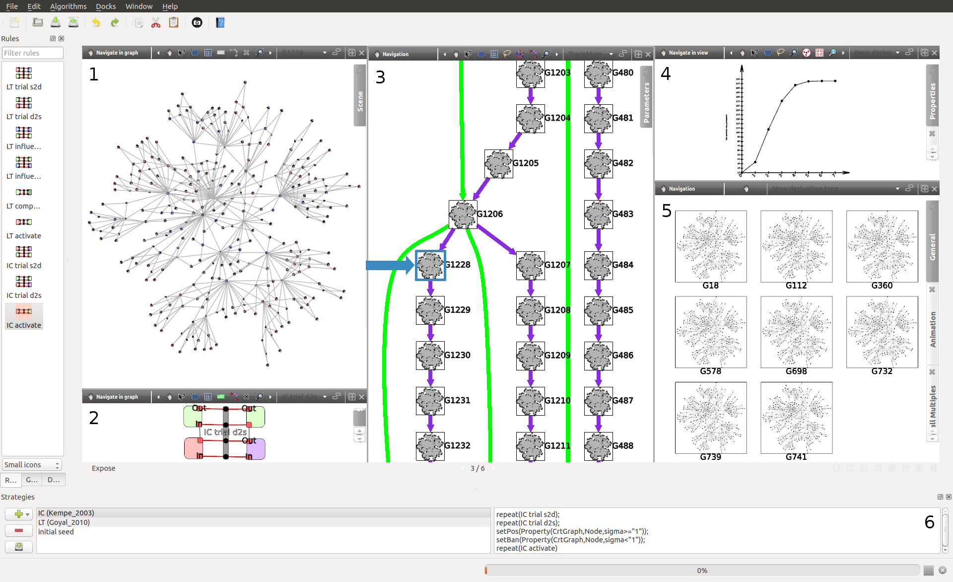
Figure 1: PORGY Interface: (1) the social network on which we apply the propagation; (2) rule edition; (3) part of the derivation tree (DT), used to keep a complete trace of the performed computations (e.g. graph (1) is node $G1228$); (4) curve showing the number of active nodes evolution along a branch of DT; (5) another possible representation of a branch of DT; (6) strategy editor.

This paper is organized as follows. We first present the terminology used to address social network propagation and describe two well-known models (Section 2). Then, after a brief introduction to the graph rewriting technique used, we show how propagation models are translated in our formalism to show the expressiveness and usability of graphs, rules and strategies (Section 3). Finally, we show how the platform PORGY is used to study the propagation models and exhibit some differences (Section 4) and conclude by giving a few perspectives and future work directions.

2 Propagation modelling in social networks

A social network  [3] is a graph $G=(V,E)$ built from a set of individuals (the nodes) $V$ and a set of edges $E\subseteq V\times V$ linking individuals and indicating a mutual recognition. Two individuals, $v,w\in V$, are called neighbours when linked by an edge $e\in E$; we define $N(w)$ the set of neighbours of the node $w$. Propagation in a network can be seen as follows: when an individual performs a specific action (announcing an event, spreading a gossip, sharing a video clip, etc.), she/he becomes active. She/He informs his neighbours of his state change, giving them the possibility to become active if they perform the same action. Such process reiterates as the newly active neighbours share the information with their own neighbours. The activation can thus propagate from peer to peer across the whole network.

This definition is obviously simplified since each existing propagation model has its own specificities to be the most efficient in replicating the phenomena observed in real-world networks. Hence some models opt for entirely probabilistic activations (e.g. [5, 38]) where the presence of only one active neighbour is enough to allow the propagation to occur. Other models use threshold values (e.g. [37, 24, 16]) building up during the propagation. Such measures can be used to gauge the influence of one individual on his neighbours or represent his tolerance towards performing a given action (the more one individual is solicited, the more she/he becomes inclined to activate or not).

Because of the diversity across existing models and due to limited space, we limit the range of this paper to illustrate the feasibility of our approach on two representative models: an independent cascade model IC [23] used as basis in numerous others, and a linear threshold model LT [16] using a non-probabilistic activation principle in opposition to the independent cascade.

The independent cascade model (IC).

We describe a basic form as introduced in [23].

• Let $A_{0}\subset V$ be the subset of nodes initially activated at $t=0$.

• Let $p_{v,w}$ be defined for each pair of adjacent nodes $\{v,w\}$ to characterize the influence probability from $v$ on $w$ ($0\leq p_{v,w}\leq 1$). $p_{v,w}$ is considered as being history independent and non symmetric, that is we usually have $p_{v,w}\not=p_{w,v}$.

• A new set of nodes $A_{t+1}$ is computed from $A_{t}$ such as, for each $v\in A_{t}$, we visit the nodes $w$ adjacent to $v$ but still inactive such as $w\in N(v)\setminus\cup_{i=0}^{t}A_{i}$. A given node $v$ is only offered one chance to influence each of its neighbours, following a probability $p_{v,w}$. When the adjacent node $w$ is successfully activated, it is added to $A_{t+1}$.

• This process continues until $A_{t+k}$ is empty ($\varnothing$) for $k\geq 0$.

The order used to choose the nodes $v$ and their neighbours is arbitrary. This model has several variations (e.g. [15, 37]) to allow for instance to simulate the propagation of diverging opinions in a social network [5].

The linear threshold model (LT).

This model behaves differently, using the neighbours’ combined influence and threshold values to determine whether a node becomes active or stays in the same state. A partial list of publications describing models using thresholds is available in [23]. The model detailed below describes the first static model defined in [16].

• $A_{0}\subset V$ remains the subset of nodes initially activated at $t=0$. We also consider the probabilities $p_{v,w}$ previously introduced and add a threshold value $\theta_{w}$ to define $w$’s resistance to its neighbours’ influence.

• We define $S_{w}$ as the set of nodes currently active and adjacent to $w$. For each inactive node $w$, we compute its neighbours’ joint influence value $p_{w}(S_{w})=1-\prod_{v\in S_{w}}(1-p_{v,w})$.

• $w$ becomes active when its neighbours’ joint influence exceeds the threshold value, $p_{w}(S)\geq\theta_{w}$, and $w$ is then added to $A_{t+1}$.

• Those instructions are repeated until $A_{t+k}$ is empty ($k\geq 0$).

3 Models translation and rewriting rules

This section describes the formalism used to express in a uniform algorithmic language the various models mentioned in the previous section.

Graphical formalisms are useful to easily describe complex structures in an intuitive way, like UML diagrams, proof representation, micro-processors design, work-flows, etc. Extensive work exists on visual representation and information visualization; we refer the reader to [36] for a perception-oriented approach, and [35] for a more technical and applicative direction.

From a theoretical point of view, graph rewriting has solid logic, algebraic and categorical foundations [8, 30], while from a practical perspective, graph transformations have many applications in specification, programming, and simulation tools [11, 12]. Graph rewriting conveniently offers both semantical and operational frameworks for distributed systems and modelling complex systems in general. Several languages and tools are based on this formalism, such as PROGRES [32], GROOVE [29], GrGen [14] or GP [28].

3.1 Graph rewriting using port graphs

Graph rewriting is a graph transformation described by rules, applied in a proper order specified by a strategy. A rewrite rule is given by two graphs $L$ and $R$, respectively called the left-hand side and right-hand side. In a given graph $G$, the left-hand side of the rule –describing a pattern– is used to identify corresponding subgraphs which should be replaced by the right-hand side of the rule. Different techniques can be used to describe the relation between $L$ and $R$, especially how the elements in the right-hand side replace those in the left-hand side and become connected to the rest of the graph. The method chosen in our solution makes use of port graphs, allowing the definition of such informations directly in the rewriting rules.

3.1.1 Port graph with properties

Intuitively, a port graph is a graph where nodes have explicit connection points called ports. A port graph $G$ is defined by a finite set $N$ of nodes $n$, a finite set $P$ of ports $p$ (each depending from a given node of $N$) and a finite set $E$ of undirected edges. They are exclusively attached to ports and two ports may be connected by more than one edge.

Nodes, ports and edges are labelled with a set of properties. For instance, an edge may be associated with a state (e.g. used or marked) and a node may have a colour, a number and a label as properties. Properties may be used to define the behaviour of the modelled system and for visualization purposes (as illustrated in examples later).

Formally, properties are pairs $(a,v)$ of an attribute $a$ and a value $v$ whose types are described in a signature. We write $a=v$ to mean that the attribute $a$ has the value $v$: for example, $active=yes$, $colour=blue$, $resist=3$ and $size=x$ (in the latter example we use the variable $x$ to mean that we do not care what the value of $size$ is, just that the attribute exists). A record $r$ is a set $\{(a_{1},v_{1}),\ldots,(a_{n},v_{n})\}$ of properties, where each $a_{i}$ occurs only once in $r$. All elements in $N$, $P$ and $E$ are labelled by records defining their properties.

In this paper, to represent a social network, we use a port graph whose nodes represent individuals. Among the properties attached to a node are for instance the properties $visited$ and $active$ which both take boolean values. Edges may also have properties. The model described in Section 3.2.1 uses a boolean property, marked, on an edge to know if a pair of adjacent nodes has been visited or not. Other properties of nodes and edges will be introduced later to model propagation effects.

The port graph representation uses undirected edges, however, ports can be used to simulate edge orientation. By defining two ports on each node, named $In$ and $Out$, an edge becomes directed as it leaves a node through an $Out$ port and reaches its destination using an $In$ port. In our case, we limit to one the number of edges connecting any two ports. An edge between the $In$ port of node $A$ and the $Out$ port of node $B$ indicates that $A$ and $B$ are linked and can influence each other, regardless of the edge direction. The edge orientation allows us to use only one edge to store different properties. If $B$ influences $A$ (going from $Out$ to $In$), the corresponding value is quantified in the attribute $p_{o2i}$, expressed as a rational number; while the influence of $A$ applied on $B$ (from $In$ to $Out$) will be stored in $p_{i2o}$.

3.1.2 Port graph rewrite rule

Port graphs are transformed by applying port graph rewrite rules. A port graph rewrite rule, noted $L\Rightarrow R$, is itself a port graph, consisting of two sub-port graphs, $L$ and $R$, connected together through one special port node $\Rightarrow$, called arrow node. This unique node describes how the new subgraph should be linked to the remaining part of the graph to avoid dangling edges [18, 7] during rewriting operations.

Simple rewrite rules used in this paper are given in Figure 2. An arrow node, coloured in grey, has a number of black ports each possessing an attribute type and a set of red arrow edges. These edges, connecting a port of the arrow node to ports in $L$ or $R$, are used to control the rewiring that occurs during a rewriting step. The ports of type bridge, similar to those used in our example, form a bridge between both sides of the rewrite rule, and indicate that the corresponding port in $L$ survives the rule application. Other types of ports correspond to more specific situations (merging, deletion, etc.) but are not relevant in this paper. Altogether, they are meant to manage the edges existing between $L$ and the rest of the graph during rewriting operations.

We need to enrich this port graph structure by allowing an additional feature to rules: each attribute’s value in the properties of nodes, ports and edges of the right-hand side may be a function of attribute’s value in the properties of nodes, ports and edges of the left-hand side. In this way, each transformation applied as a port graph rewrite rule is completed with the application of rule-specific functions $f$ designed to modify the attribute’s values of each element (whether they are nodes, ports or edges). However this remains a local computation since the arguments are taken from the properties of the homomorphic image of the left-hand side. Formally, this amounts to considering values of properties which are no more constants in a finite domain but functions of several arguments. This functionality is demonstrated in Section 3.2.1 where we introduce a node’s attribute $sigma$, whose value in the right-hand side is computed from several properties originating from different elements of the left-hand side.

3.1.3 Rewrite strategy

To perform the appropriate graph transformations, the rules have be to applied in a precise order. It is the purpose of the strategy to specify which rules to apply, in which order and how many times.

A strategy may also be used to depict which elements can be considered for the rewriting operations (matching and replacement) and which ones are forbidden. This is achieved through an additional refinement of port graphs and port graph rewrite rules. A located graph $G_{Pos}^{Ban}$ consists of a port graph $G$ and two distinguished subgraphs $Pos$ and $Ban$ of $G$, called respectively the position subgraph, or simply position, and the banned subgraph.

In a located graph $G_{Pos}^{Ban}$, $Pos$ represents the subgraph of $G$ where rewriting steps may take place (i.e., $Pos$ is the focus of the rewriting) and $Ban$ represents the subgraph of $G$ where rewriting steps are forbidden. The intuition is that subgraphs of $G$ that overlap with $Pos$ may be rewritten only if they are outside $Ban$, thus restricting the application of rules to explicit elements. $Pos$ and $Ban$ are not exclusively sets of nodes but may also contain edges or ports.

For instance, in a social network context, we may consider a rule that makes a node becoming active and limit its application to nodes whose level of incentive is above a given threshold. This is done through a strategy $setPos$ that selects the adequate subgraph.

When applying a port graph rewrite rule, not only the underlying graph $G$ but also the position and banned subgraphs may change. A located rewrite rule specifies two disjoint subgraphs, $J$ and $K$ of the right-hand side $R$, and manipulates these to update the position and banned subgraphs (respectively). If $J$ (resp. $K$) is not specified, $R$ (resp. the empty graph $\emptyset$) is used as default.

More details on the strategy language implemented in the PORGY platform, its general formalisation and properties can be found in [13].

3.2 Translation of propagation models

Our main challenge concerns the translation of a given propagation model into a set of rules and an adequate strategy allowing to reproduce the model behaviour. Graph rewriting techniques offer us to perform virtually any possible transformation with an appropriate rewrite rule, so one can always create a rule corresponding to its need. The real difficulty is to understand whether a finite set of rules and strategies could describe different propagation models and their behaviours.

After a careful study of a wide range of models, we have realized the feasibility of such task, since all considered models are based on either the independent cascade or the linear threshold models. The work developped in [23] which proposes a framework unifying those two models open the way, showing that a proper generalization can bring together the two models, thus reducing the differences to mere variations. As we consider a finite number of differences between the two basic models and any other based on those, if one can express the IC or the LT model using a graph rewriting formalism (under the form of a strategy controlling a finite set of rules), any variation based on these models can also be expressed. Consequently, starting from the basic model translation, any extended model rendering can be accomplished with the introduction of a finite number of additional rules –to describe the differences between the currently studied model and the basic one– and a few adjustments in the strategy to order rule applications.

We present below the translation of the IC and LT models thus providing instructions and showing how one should proceed to obtain similar results with different variations.

3.2.1 Model IC

Using the model definition introduced in Section 2, one can easily notice the two main operations to perform. The first one is the influence trial where a given active node $v$ tries to influence an inactive neighbour $w$. The activation of $w$, once it has been successfully influenced, is the second operation. Following the model description, these two instructions need to be applied one after the other to emulate the propagation process properly.

Rule translation

The corresponding rules are given in Figure 2. Rule 2(a) shows a pair of connected nodes in the left-hand side and their corresponding replacements in the right-hand side. The ports from each side are connected with red edges through the bridge port (as explained in Section 3.1.2). The node $w$, initially inactive (in red), is influenced –successfully or not– in the left-hand side by an active node $v$ (green). In the right-hand side, $w$ becomes purple to indicate visually that it has been visited, while $v$ is not modified. Finally, the edge linking the two port nodes is marked using a boolean attribute. This is to limit the number of influence attempts to one for each pair of active/inactive neighbours. Thus, the inactive node can be visited by different active neighbours and be influenced several times. Rule 2(b) is only applied on a single node. If $w$ has been previously sufficiently influenced by one of its neighbours, its state is changed, going from visited (purple) to active (green).

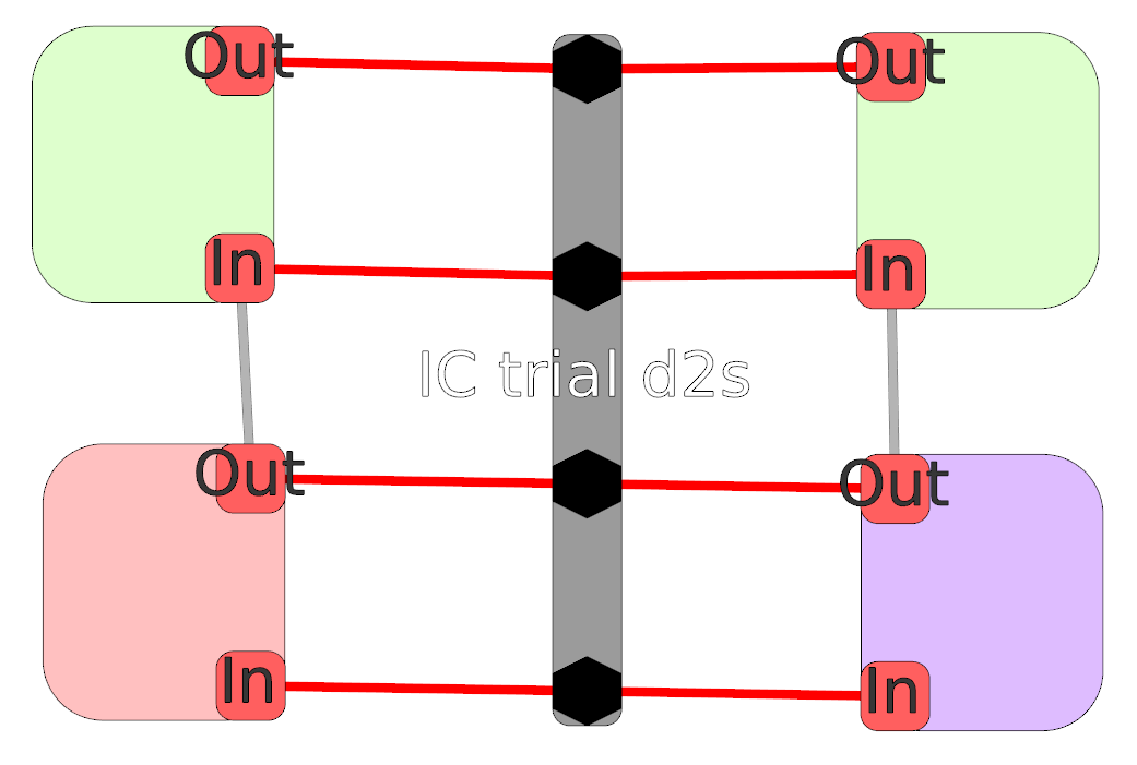
(a) Influence trial from an active neighbour

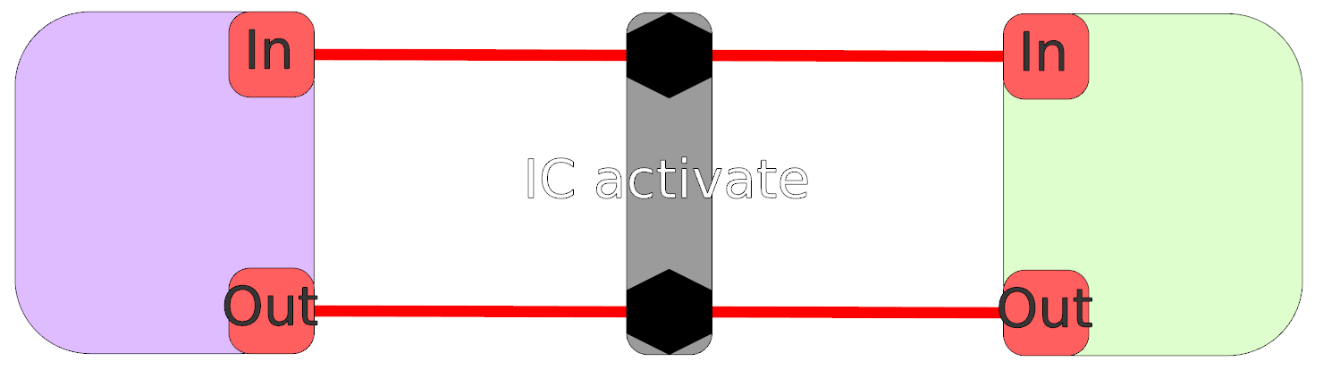
(b) Visited node activation

Figure 2: Rules used to express the IC model. Active nodes are depicted in green and visited nodes in purple. Red nodes are in an inactive state (however, they may have been visited already).

Emulating edge orientation

For any pair of adjacent nodes $a$ and $b$, both influence probabilities $p_{a,b}$ (from $a$ to $b$) and $p_{b,a}$ (from $b$ to $a$) are defined as properties of the edge linking $a$ to $b$. The two influence probabilities being different, we wish to dissociate one individual from another (knowing which node is which) in order to use the appropriate value. As explained in Section 3.1.1, edges in port graphs are not directed, preventing to use edge orientation as a referential to distinguish the influence probabilities (one property for source to destination influence and another one for destination to source influence). Ports In and Out are used to emulate such edge orientation: an edge leaves by the Out port and arrives through the In port. The two properties keeping the influence probabilities, $p_{i2o}$ (In to Out) and $p_{o2i}$ (Out to In), are stored on each edge. In Rule 2(a), an edge leaves an inactive node by its Out port and reaches an active one through its In port. The influence going from an active to an inactive node (in this case, from In to Out), we will hence use the value stored in $p_{i2o}$ (=$p_{v,w}$). To cope with the other possibility (going from the active node to the inactive one in an Out to In direction), the rule is “duplicated” and the ports’ labels are switched. While not presented here, this orientation is similar to the one encountered in the rule in Figure 3(a).

Rule inner function

The sole execution of these rules is insufficient to perform a propagation. The use of the rule inner function $f$, introduced by the end of Section 3.1.2, allows us to perform additional local modifications to the elements concerned by the rule application. For instance, in Rule 2(a), for each pair active($v$)/visited($w$): a) we generate a random number $r\in]0,1]$ ; b) we store in a property $\sigma_{w}$ the maximum influence withstood by $w$ from its active neighbours until now (initialized to $0$) such as $\sigma_{w}=\max\left(\frac{p_{v,w}}{r},\sigma_{w}\right)$ ; and c) through a boolean property, we mark the edge linking $v$ to $w$ to prevent the selection of this peculiar pair configuration in the next pattern matching searches. This means that an active node $v$ will not be able to try to influence the same node $w$ over and over. Those local modifications, expressed through the function $f$, are applied on the resulting elements (from the right-hand side), using the initial element properties. If we define the left-hand side nodes, $v$ and $w$, and their right-hand side equivalents, $v^{\prime}$ and $w^{\prime}$, the $\sigma$ computation is expressed as:

⬇

node(w’).property(”sigma”) =

max(edge(v,w).property(”p_v,w”)/random(1),

node(w).property(”sigma”));

We affect to the property $sigma$ of the right-hand side node $w^{\prime}$ the maximum between the value of the property $sigma$ of the $w$ element and the result of the fraction $\frac{p_{v,w}}{r}$, where $p_{v,w}$ is obtained from the property $p\_v,w$  of the edge $\{v,w\}$ and $random(X)$ returns an arbitrary value between $0$ and $X$. This function is locally applied after each successful application of the rule. Once every active neighbour has been tried, if $w$ is sufficiently influenced ($\sigma_{w}>1$), it becomes itself active with Rule 2(b).

Strategy and rule application

The successive applications of the rules describing the IC model have to be managed by a strategy. As mentioned earlier, the strategy can be for example used to precisely select or exclude elements as possible candidates for a rule application. The rewriting strategy used to represent the IC model is as follows:

⬇

1repeat(IC trial d2s);

2repeat(IC trial s2d);

3setPos(Property(CrtGraph,Node,sigma>=”1”));

4repeat(IC activate)

The first two instructions (line 1-2) are used to call the influence trial rules successively until every pair of active/inactive neighbours has been considered. Then (line 3), the positions in the graph where the activation should take place are selected as the nodes in the current graph whose property “sigma” is greater or equal to 1, according to our translation of the propagation model. Line 4 executes repeatedly the activation rule at these positions. For each rule application, the elements corresponding to the left-hand side are chosen arbitrarily among the matching possibilities. A successful and complete application of this strategy performs a round of propagation: we try to influence every susceptible node, then activate all the appropriately influenced ones at the same time. This process is reiterated to obtain successive waves, similar to ripples. A more progressive behaviour can be observe by simply applying the activation rule after each influence trial. Because the choice of each pair of active/inactive nodes is arbitrary, such activation process can be seen as a “random” propagation. However, due to limited space, this kind of propagation evolution is not addressed in this paper.

3.2.2 Model LT

The second model seems more complicated but the approach is very similar. Here again, two different operations are used to perform the propagation: for each inactive node, we compute the joint influence of its active neighbours, then, if the influence exceeds the threshold value, the node becomes active.

Before presenting the corresponding rules, a few precisions need to be highlighted concerning this model described in [16]. The paper presents, among others, a static propagation model with several variations. We need to define the probability of $v$ influencing $w$ ($p_{v,w}$), however, such probability of influence from one individual to another may change from time to time (additional details are given in [16]). Because the activation of a specific node $w$ is dependent of the probabilities emanating from each of its neighbours, we need to keep their joint influence $p_{w}(S_{w})$ updated.

Such correction can be performed using the two operations $p_{w}(S_{w}\setminus\{u\})$ (Equation 1), suppressing the influence of $u$ on $w$ among its neighbours ($S_{w}$), and $p_{w}(S_{w}\cup\{u^{\prime}\})$ (Equation 2), adding the influence of $u^{\prime}$ among the other adjacent nodes of $w$.

$$p_{w}(S_{w}\setminus\{u\})=\frac{p_{w}(S_{w})-p_{u,w}}{1-p_{u,w}}$$ (1)

$$p_{w}(S_{w}\cup\{u^{\prime}\})=p_{w}(S_{w})+(1-p_{w}(S_{w}))*p_{u^{\prime},w}$$ (2)

An improvement, introduced in [16], gives the opportunity to update the joint influence in a single operation. The two manipulations on the set $S_{w}$ –deleting the previous influence probability value with Equation 1 and adding the new one using Equation 2– can be perform simultaneously: $p^{\prime}_{w}(S_{w})=p_{w}(\{S_{w}\setminus\{u\}\}\cup\{u^{\prime}\})=p_{w}(\{S_{w}\cup\{u^{\prime}\}\}\setminus\{u\})$.

Rules and strategy

The rules created from this model are quite similar to those introduced before. The first one (Figure 3(a)) is applied on a pair of active/inactive nodes (respectively green and red). It comes in two variations depending of the In/Out port used. As we consider the possibility of an updated influence probability from $v$ to $w$ ($p_{v,w}$), when trying to activate, $w$ has to refresh the joint influence ($p_{w}(S)$) of its neighbours. The inner function performed when the rule is applied computes $p^{\prime}_{w}(S)=p_{w}(\{S\setminus\{u\}\}\cup\{u^{\prime}\})$, where $u$ is the neighbour using its previous influence probability and $u^{\prime}$ is the node with the updated value. For each application, a $\sigma_{w}$ value is also calculated as follows: $\sigma_{w}=\frac{p_{w}(S)}{\theta_{w}}$, so it becomes greater or equal to $1$ when $w$ is ready to activate ($\theta_{w}$ –stored in a property– being the threshold value that the joint influence $p_{w}(S)$ must reach for $w$ to activate). The second Rule 3(b) is per se identical to the activate rule shown in Figure 2(b). A successfully influenced node is simply activated; the strategy alone is used to delimit the nodes eligible for activation.

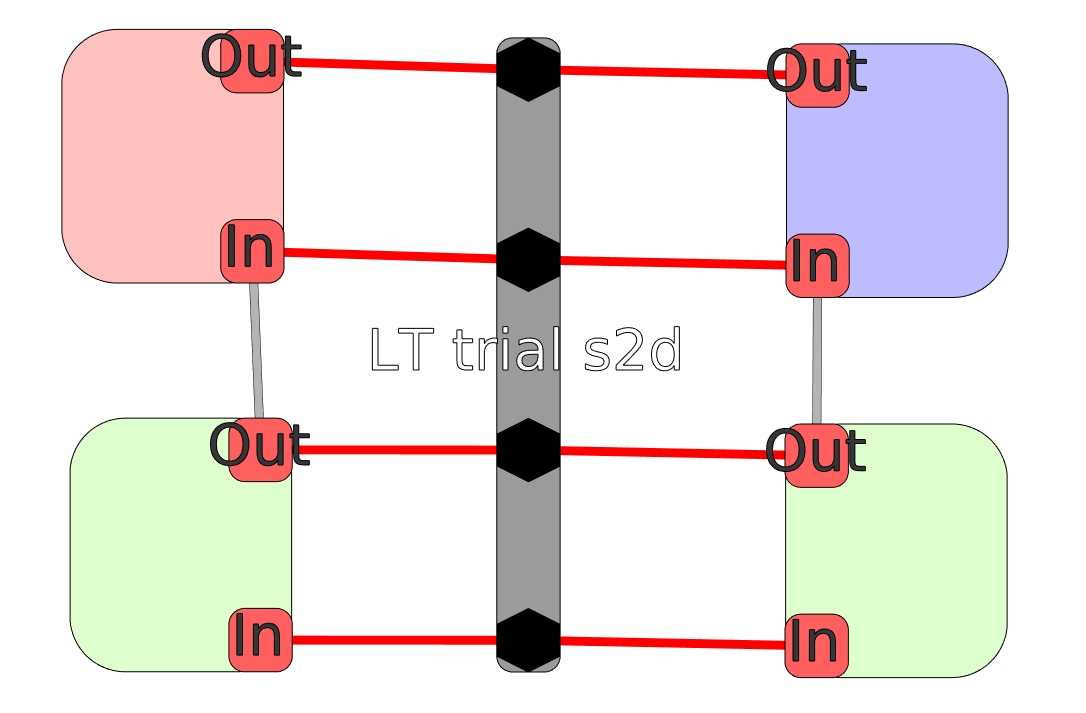
(a) Joint influence computation from an active neighbour

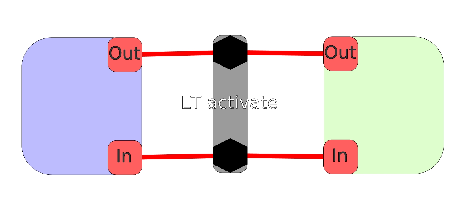
(b) Influenced node activation

Figure 3: Rules used to express the linear threshold model. Colours conserve the same meaning as previously: active nodes are green, visited nodes are purple and red nodes are inactive (but may have been already visited).

Like the IC model, the first two rules are applied successively on the graph to evaluate every active/inactive pair. The “sigma” property is once more used to determine upon which nodes the activation must be performed. Eventually, the activation rule is applied as many times as needed:

⬇

1repeat(LT trial s2d);

2repeat(LT trial d2s);

3setPos(Property(CrtGraph,Node,sigma>=”1”));

4repeat(LT activate)

Alike the previous model, successive applications of the strategy creates rounds of propagations. If one wishes to obtain a more progressive and irregular behaviour, the activation rule must be applied after each influence trial.

4 Visual analytics and model comparison

We detail in this section how the PORGY platform is used to compare two series of propagations from the independent cascade and linear threshold models. To illustrate our method, we create a random social network using the graph generation model introduced in [34]. The resulting graph contains 300 nodes (chosen as a parameter) and 597 edges (defined by the generator). The starting conditions are similar for the two propagation models: same set of initially active nodes and same starting values for the different properties needed by the models (e.g. influence probability distribution, threshold value, …). We do not aim here at showing if a given model is better or more realistic than another one, as such task needs numerous simulations to compute the average results on the probabilistic models and extensive comparisons with real-world cases. Moreover, the considered propagation models have already been validated in that respect. Instead, we want to understand how models evolve and behave.

4.1 Network evolution and history

Upon each rule execution, an intermediate state of the original graph is created and stored in the propagation trace, thus keeping track of the changes applied to each node and edge in the graph, for instance nodes going from unvisited to visited and possibly active. The history of those modifications, or rewriting steps, can be used to study and compare two states of the graph at a given time or to rebuild and follow the path of node activation.

A derivation tree (see Figure 1) is created and maintained to provide these information. To improve readability, several rule applications are grouped together according to the strategy execution and considered as one propagation step. The successive states visualization allows us to witness this progression. Figure 4 presents several representations of the same subgraph, showing node states evolution. The different timestamps $t$ indicate the successive strategy applications (an unvisited node at time $t$ can thus become activated at $t+1$).

The derivation tree allows us to immediately identify the model which needs the less propagation steps (i.e. less strategy application steps) before concluding the propagation, since it corresponds to the shorter branch (Figure 5). We thus obtain a first complexity approximation concerning algorithms execution.

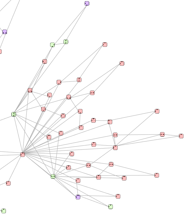
(a) $t=1$

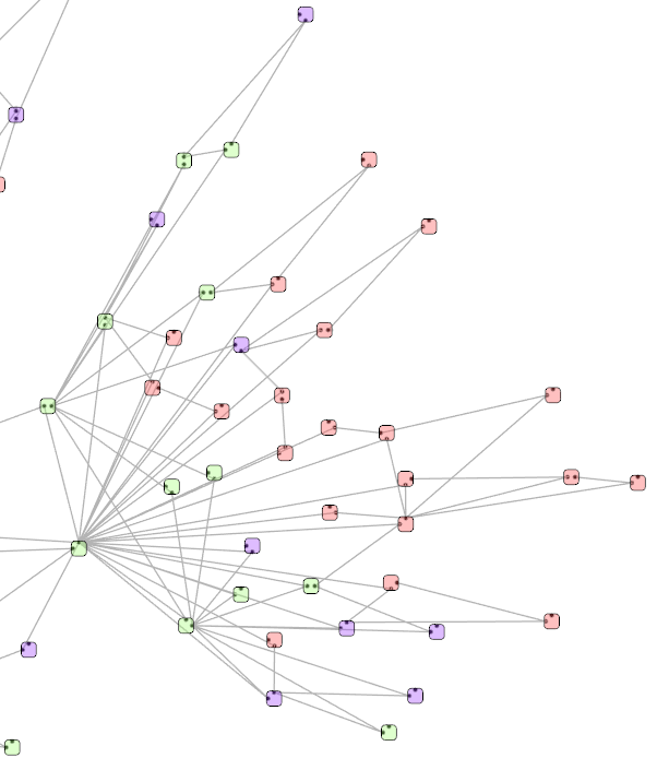
(b) $t=2$

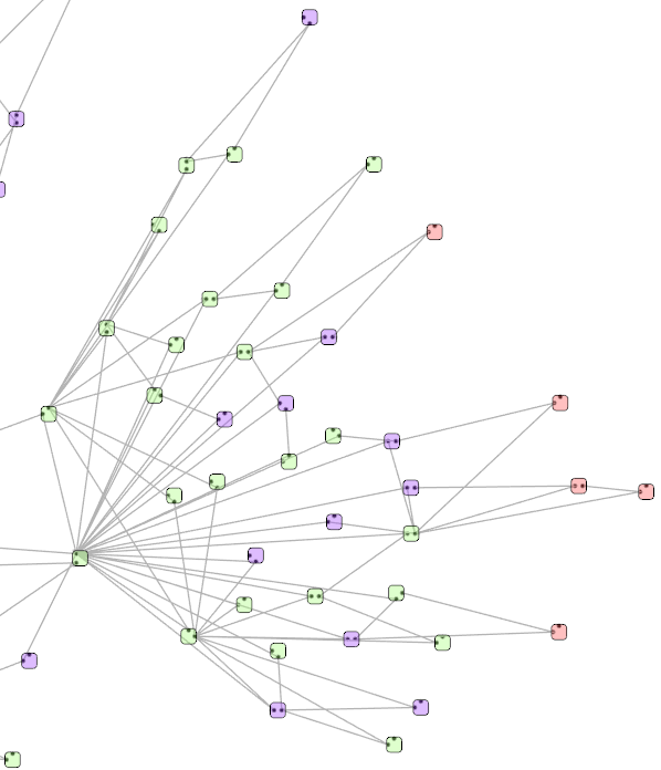
(c) $t=3$

Figure 4: Sub-community extracted from the graph showing the propagation evolution at different time steps. Two nodes are activated at $t=0$ (not showed here) and six are only visited at the end of the propagation (at $t=7$). (Legend: green = active, purple = visited, red = unvisited and inactive)

4.2 Statistics

Linking the derivation tree depth (equivalent to the number of propagation steps along a branch) with other measures allows us to consider the evolution of several parameters all along the propagation. We can, for instance, use the notion of propagation speed, a value obtained by examining the number of active nodes at each step and evaluate their evolution. Figure 5 presents such measures for an independent cascade model ((2), top right panel) and a linear threshold model ((3), bottom right panel) executions. The x-axis displays the depth (maxed out at $7$ for (2) and at $4$ for (3)) and the y-axis the number of active nodes (scaling from $0$ to $300$ in both curves). We can notice that the cascade model has been able to activate approximately $80\%$ of its nodes versus $18\%$ for the threshold model (for a similar number of steps), thus showing the high performance impact on different models when using identical values for the influence probability initialization and the same starting set of active nodes. We have used a magnifying glass (a functionality available in PORGY) on the top of both axes to improve the scale readability. We can also note the number of activated nodes after the first strategy application. The values measured on both scatterplots are initially close, the gap between the two models getting wider with each new application.

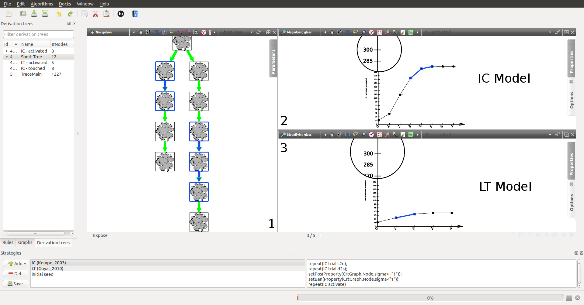
Figure 5: PORGY interface: (1) portion of a simplified derivation tree (filtered to show only the results obtained after a whole strategy application) ; (2) and (3) Propagation speed evolution (number of active nodes) according to the depth in the derivation tree branch for the independent cascade (IC) and linear threshold (LT) models.

Moreover, time-dependent measures can be generalized to other propagation properties. The notion of visited nodes, introduced earlier, can bear some interest when the propagation subject is only a message which needs to be seen and not merely disseminated or spread by willing individuals. Such acknowledgement speed of the propagation content can be determined like the propagation speed. Moreover, considering those two measures, we can introduce a third one defining the propagation efficiency, computed as the ratio of the number of active nodes at time $t$ against those influenced/visited at $t-1$. Several additional metrics can be computed depending of the wished analysis as PORGY offers us to choose any of the existing element property and traces its evolution through the derivation tree.

4.3 Tracing propagation behaviour

One can also be interested in observing the state of the social network when the number of activated nodes reaches a given value. Because the different views in the software are linked together, any operation in one view impacts the other views. A node/edge selection (highlighted in blue in Figure 5) in the derivation tree implies the same in the scatterplot and vice versa. A similar kind of operation in one of the graph states will echo through all the states containing the same elements, thus highlighting the selected nodes/edges everywhere they are. Such behaviour is available thanks to the inner datastructure of PORGY, leaving the nodes unmodified as long as they are not subject to a rule application. Consequently, selecting an element of interest in one of the intermediate graphs allows us to follow and determine in which state this element is altered. Such operation is especially useful when working with the complete derivation tree (showing the details of every rule application).

Using the final propagation state, one can witness whether or not a node has finally been able to perform the action (activated). Identifying the influenced but inactive node and the unvisited elements may also help in finding the nodes responsible for limiting the propagation. Once the wrongdoers have been found, specific treatments can target them in order to improve their condition (i.e. lowering their resistance or rising their neighbours’ influence). A new simulation can then be launch to check if the modifications have been successful.

5 Conclusion and future work

We have presented a graph rewriting based formalism seen as a common language to express network propagation models. When the propagation does not imply topological modifications in the graph, models can be described as a reduced set of transformation rules used to express network state transitions and a strategy to manage their application.

In order to demonstrate the generality of our approach, we plan to use more propagation models and multiply the number of simulations. Simulating propagation using our method may be performed on large networks as well. Nevertheless, this raises additional challenges concerning the scalability of our approach and the possible visual analysis. The search for left-hand side matching (graph-subgraph isomorphism) is a demanding operation in big graphs even when, because of the limited number of elements in the rules left-hand side, the time complexity is polynomial.

Looking for propagation minimization or maximization on large networks by visual means may also be impeded by the combinatorial explosion of possible states thus limiting such operations. In general, visualization of large graphs is a complicated issue. Resorting to node-link views, such as the ones presented in this paper, usually gives poor results when the number of nodes or edges exceeds a few thousands. Alternative solutions, such as matrix-based hybrid [19, 31] or pixel-oriented [21] visualizations may become satisfying substitutes.

We also plan to provide more advanced network evolution models which support topology evolution and realistic information propagation behaviour. In such cases, we need at least an extended strategy language to control the simultaneous or alternate (probabilistic) applications of topological modifications or propagation rules.

Acknowledgement

This work has been partially financed by ANR JCJC EVIDEN (2010-JCJC-0201-01) grant. We would also like to thank the anonymous reviewers for their detailed comments and helpful suggestions.

References

- [1]
- [2] E. Bertuzzo, R. Casagrandi, M. Gatto, I. Rodriguez-Iturbe & A. Rinaldo (2010): On spatially explicit models of cholera epidemics. J. of The Royal Society Interface 7(43), pp. 321–333, 10.1098/rsif.2009.0204.
- [3] U. Brandes & D. Wagner (2004): Analysis and Visualization of Social Networks. In Michael Jünger & Petra Mutzel, editors: Graph Drawing Software, Mathematics and Visualization, Springer Berlin Heidelberg, pp. 321–340, 10.1007/978-3-642-18638-7_15.
- [4] P. J. Carrington, J. Scott & S. Wasserman (2005): Models and Methods in Social Network Analysis. Structural Analysis in the Social Sciences, Cambridge University Press, 10.1017/CBO9780511811395.
- [5] W. Chen, A. Collins, R. Cummings, T. Ke, Z. Liu, D. Rincón, X. Sun, Y. Wang, W. Wei & Y. Yuan (2011): Influence Maximization in Social Networks When Negative Opinions May Emerge and Propagate. In: SIAM Int. Conf. on Data Mining, SDM, pp. 379–390, 10.1137/1.9781611972818.33.
- [6] W. Chen, C. Wang & Y. Wang (2010): Scalable Influence Maximization for Prevalent Viral Marketing in Large-scale Social Networks. In: ACM SIGKDD Int. Conf. on Knowledge Discovery and Data Mining, KDD ’10, pp. 1029–1038, 10.1145/1835804.1835934.
- [7] A. Corradini, U. Montanari, F. Rossi, H. Ehrig, R. Heckel & M. Löwe (1997): Algebraic Approaches to Graph Transformation - Part I: Basic Concepts and Double Pushout Approach. In: Handbook of Graph Grammars and Computing by Graph Transformations, Volume 1: Foundations, World Scientific, pp. 163–246, 10.1142/9789812384720_0003.
- [8] B. Courcelle (1990): Graph Rewriting: An Algebraic and Logic Approach. In J. van Leeuwen, editor: Handbook of Theoretical Computer Science (Vol. B), MIT Press, Cambridge, MA, USA, pp. 193–242. Available at http://dl.acm.org/citation.cfm?id=114891.114896.
- [9] P. S. Dodds & D. J. Watts (2005): A generalized model of social and biological contagion. J. of Theoretical Biology 232(4), pp. 587–604, 10.1016/j.jtbi.2004.09.006.
- [10] P. Domingos & M. Richardson (2001): Mining the Network Value of Customers. In: ACM SIGKDD Int. Conf. on Knowledge Discovery and Data Mining, KDD ’01, pp. 57–66, 10.1145/502512.502525.
- [11] H. Ehrig, G. Engels, H.-J. Kreowski & G. Rozenberg, editors (1997): Handbook of Graph Grammars and Computing by Graph Transformations, Volume 2: Applications, Languages, and Tools. World Scientific.
- [12] H. Ehrig, H.-J. Kreowski, U. Montanari & G. Rozenberg, editors (1997): Handbook of Graph Grammars and Computing by Graph Transformations, Volume 3: Concurrency, Parallelism, and Distribution. World Scientific.
- [13] M. Fernandez, H. Kirchner & B. Pinaud (2014): Strategic Port Graph Rewriting: An Interactive Modelling and Analysis Framework. In Dragan Bošnački, Stefan Edelkamp, Alberto Lluch Lafuente & Anton Wijs, editors: GRAPHITE 2014, EPTCS 159, pp. 15–29, 10.4204/EPTCS.159.3.
- [14] R. Geiß, G. V. Batz, D. Grund, S. Hack & A. Szalkowski (2006): GrGen: A Fast SPO-Based Graph Rewriting Tool. In A. Corradini, H. Ehrig, U. Montanari, L. Ribeiro & G. Rozenberg, editors: Graph Transformations, Lecture Notes in Computer Science 4178, Springer Berlin Heidelberg, pp. 383–397, 10.1007/11841883_27.
- [15] M. Gomez-Rodriguez, J. Leskovec & A. Krause (2010): Inferring Networks of Diffusion and Influence. In: ACM SIGKDD Int. Conf. on Knowledge Discovery and Data Mining, KDD ’10, pp. 1019–1028, 10.1145/1835804.1835933.
- [16] A. Goyal, F. Bonchi & L. V. S. Lakshmanan (2010): Learning Influence Probabilities in Social Networks. In: ACM Int. Conf. on Web Search and Data Mining, WSDM ’10, pp. 241–250, 10.1145/1718487.1718518.
- [17] M. Granovetter (1978): Threshold Models of Collective Behavior. American J. of Sociology 83(6), pp. 14–20, 10.1086/226707.
- [18] A. Habel, J. Müller & D. Plump (2001): Double-pushout graph transformation revisited. Mathematical Structures in Computer Science 11(5), pp. 637–688, 10.1017/S0960129501003425.
- [19] N. Henry, J. D. Fekete & M. J. McGuffin (2007): NodeTrix: a Hybrid Visualization of Social Networks. Transactions on Visualization and Computer Graphics, IEEE 13(6), pp. 1302–1309, 10.1109/TVCG.2007.70582.
- [20] H. Hethcote (2000): The Mathematics of Infectious Diseases. SIAM Review 42(4), pp. 599–653, 10.1137/S0036144500371907.
- [21] D. A. Keim (2000): Designing pixel-oriented visualization techniques: theory and applications. Transactions on Visualization and Computer Graphics, IEEE 6(1), pp. 59–78, 10.1109/2945.841121.
- [22] N. Kejžar, Z. Nikoloski & V. Batagelj (2008): Probabilistic Inductive Classes of Graphs. J. of Mathematical Sociology 32(2), pp. 85–109, 10.1080/00222500801931586.
- [23] D. Kempe, J. Kleinberg & É. Tardos (2003): Maximizing the Spread of Influence Through a Social Network. In: Proc. of the ACM SIGKDD Int. Conf. on Knowledge Discovery and Data Mining, KDD ’03, pp. 137–146, 10.1145/956750.956769.
- [24] D. Kempe, J. Kleinberg & É. Tardos (2005): Influential Nodes in a Diffusion Model for Social Networks. In Luís Caires, GiuseppeF. Italiano, Luís Monteiro, Catuscia Palamidessi & Moti Yung, editors: Automata, Languages and Programming, LNCS 3580, Springer, pp. 1127–1138, 10.1007/11523468_91.
- [25] M. W. Macy (1991): Chains of Cooperation: Threshold Effects in Collective Action. American Sociological Review 56(6), pp. 730–747, 10.2307/2096252. ISSN: 0003-1224.
- [26] M. Newman, A.-L. Barabási & D. J. Watts (2006): The structure and dynamics of networks. Princeton Studies in Complexity, Princeton University Press. Available at http://books.google.fr/books?id=6LvQIIP0TQ8C.
- [27] B. Pinaud, G. Melançon & J. Dubois (2012): PORGY: A Visual Graph Rewriting Environment for Complex Systems. Computer Graphics Forum 31(3), pp. 1265–1274, 10.1111/j.1467-8659.2012.03119.x.
- [28] D. Plump (2009): The Graph Programming Language GP. In Symeon Bozapalidis & George Rahonis, editors: Algebraic Informatics, Lecture Notes in Computer Science 5725, Springer Berlin Heidelberg, pp. 99–122, 10.1007/978-3-642-03564-7_6.
- [29] A. Rensink (2004): The GROOVE Simulator: A Tool for State Space Generation. In JohnL. Pfaltz, Manfred Nagl & Boris Böhlen, editors: Applications of Graph Transformations with Industrial Relevance, Lecture Notes in Computer Science 3062, Springer Berlin Heidelberg, pp. 479–485, 10.1007/978-3-540-25959-6_40.
- [30] G. Rozenberg, editor (1997): Handbook of Grammars and Computing by Graph Transformation, Volume 1: Foundations. World Scientific Publishing Company.
- [31] S. Rufiange, M. J. McGuffin & C. P. Fuhrman (2012): TreeMatrix: A Hybrid Visualization of Compound Graphs. Computer Graphics Forum 31(1), pp. 89–101, 10.1111/j.1467-8659.2011.02087.x.
- [32] A. Schürr, A. J. Winter & A. Zündorf (1999): The PROGRES Approach: Language and Environment. In Hartmut Ehrig, Gregor Engels, Hans-Jörg Kreowski & Grzegorz Rozenberg, editors: Handbook of Graph Grammars and Computing by Graph Transformation, World Scientific Publishing Co., Inc., River Edge, NJ, USA, pp. 487–550, 10.1142/9789812815149_0013.
- [33] J. Scott & P. J. Carrington (2011): The SAGE Handbook of Social Network Analysis. SAGE Publications Ltd. Available at http://books.google.fr/books?id=mWlsKkIuFNgC.
- [34] L. Wang, F. Du, H. P. Dai & Y. X. Sun (2006): Random pseudofractal scale-free networks with small-world effect. The European Physical J. B - Condensed Matter and Complex Systems 53(3), pp. 361–366, 10.1140/epjb/e2006-00389-0.
- [35] M. O. Ward, G. Grinstein & D. A. Keim (2010): Interactive Data Visualization: Foundations, Techniques, and Applications. 360 Degree Business, CRC Press. Available at https://books.google.fr/books?id=Kk7NBQAAQBAJ.
- [36] C. Ware (2013): Information Visualization: Perception for Design. Information Visualization: Perception for Design, Morgan Kaufmann. Available at https://books.google.fr/books?id=qFmS95vf6H8C.
- [37] D. J. Watts (2002): A simple model of global cascades on random networks. Proc. of the National Academy of Sciences 99(9), pp. 5766–5771, 10.1073/pnas.082090499.
- [38] L. Wonyeol, K. Jinha & Y. Hwanjo (2012): CT-IC: Continuously Activated and Time-Restricted Independent Cascade Model for Viral Marketing. In: Proc. of ICDM, pp. 960–965, 10.1109/ICDM.2012.40.