Asymptotic Estimates in Information Theory with Non-Vanishing Error Probabilities

Abstract

This monograph presents a unified treatment of single- and multi-user problems in Shannon’s information theory where we depart from the requirement that the error probability decays asymptotically in the blocklength. Instead, the error probabilities for various problems are bounded above by a non-vanishing constant and the spotlight is shone on achievable coding rates as functions of the growing blocklengths. This represents the study of asymptotic estimates with non-vanishing error probabilities.

In Part I, after reviewing the fundamentals of information theory, we discuss Strassen’s seminal result for binary hypothesis testing where the type-I error probability is non-vanishing and the rate of decay of the type-II error probability with growing number of independent observations is characterized. In Part II, we use this basic hypothesis testing result to develop second- and sometimes, even third-order asymptotic expansions for point-to-point communication. Finally in Part III, we consider network information theory problems for which the second-order asymptotics are known. These problems include some classes of channels with random state, the multiple-encoder distributed lossless source coding (Slepian-Wolf) problem and special cases of the Gaussian interference and multiple-access channels. Finally, we discuss avenues for further research.

Part I Fundamentals

Chapter 1 Introduction

Claude E. Shannon’s epochal “A Mathematical Theory of Communication” [141] marks the dawn of the digital age. In his seminal paper, Shannon laid the theoretical and mathematical foundations for the basis of all communication systems today. It is not an exaggeration to say that his work has had a tremendous impact in communications engineering and beyond, in fields as diverse as statistics, economics, biology and cryptography, just to name a few.

It has been more than 65 years since Shannon’s landmark work was published. Along with impressive research advances in the field of information theory, numerous excellent books on various aspects of the subject have been written. The author’s favorites include Cover and Thomas [33], Gallager [56], Csiszár and Körner [39], Han [67], Yeung [189] and El Gamal and Kim [49]. Is there sufficient motivation to consolidate and present another aspect of information theory systematically? It is the author’s hope that the answer is in the affirmative.

To motivate why this is so, let us recapitulate two of Shannon’s major contributions in his 1948 paper. First, Shannon showed that to reliably compress a discrete memoryless source (DMS) $X^{n}=(X_{1},\ldots,X_{n})$ where each $X_{i}$ has the same distribution as a common random variable $X$, it is sufficient to use $H(X)$ bits per source symbol in the limit of large blocklengths $n$, where $H(X)$ is the Shannon entropy of the source. By reliable, it is meant that the probability of incorrect decoding of the source sequence tends to zero as the blocklength $n$ grows. Second, Shannon showed that it is possible to reliably transmit a message $M\in\{1,\ldots,2^{nR}\}$ over a discrete memoryless channel (DMC) $W$ as long as the message rate $R$ is smaller than the capacity of the channel $C(W)$. Similarly to the source compression scenario, by reliable, one means that the probability of incorrectly decoding $M$ tends to zero as $n$ grows.

There is, however, substantial motivation to revisit the criterion of having error probabilities vanish asymptotically. To state Shannon’s source compression result more formally, let us define $M^{*}(P^{n},\varepsilon)$ to be the minimum code size for which the length-$n$ DMS $P^{n}$ is compressible to within an error probability $\varepsilon\in(0,1)$. Then, Theorem 3 of Shannon’s paper [141], together with the strong converse for lossless source coding [49, Ex. 3.15], states that

$$\lim_{n\to\infty}\frac{1}{n}\log M^{*}(P^{n},\varepsilon)=H(X),\quad\mbox{bits per source symbol}.$$ (1.1)

Similarly, denoting $M^{*}_{\mathrm{ave}}(W^{n},\varepsilon)$ as the maximum code size for which it is possible to communicate over a DMC $W^{n}$ such that the average error probability is no larger than $\varepsilon$, Theorem 11 of Shannon’s paper [141], together with the strong converse for channel coding [180, Thm. 2], states that

$$\lim_{n\to\infty}\frac{1}{n}\log M^{*}_{\mathrm{ave}}(W^{n},\varepsilon)=C(W),\quad\mbox{bits per channel use}.$$ (1.2)

In many practical communication settings, one does not have the luxury of being able to design an arbitrarily long code, so one must settle for a non-vanishing, and hence finite, error probability $\varepsilon$. In this finite blocklength and non-vanishing error probability setting, how close can one hope to get to the asymptotic limits $H(X)$ and $C(W)$? This is, in general a difficult question because exact evaluations of $\log M^{*}(P^{n},\varepsilon)$ and $\log M^{*}_{\mathrm{ave}}(W^{n},\varepsilon)$ are intractable, apart from a few special sources and channels.

In the early years of information theory, Dobrushin [45], Kemperman [91] and, most prominently, Strassen [152] studied approximations to $\log M^{*}(P^{n},\varepsilon)$ and $\log M^{*}_{\mathrm{ave}}(W^{n},\varepsilon)$. These beautiful works were largely forgotten until recently, when interest in so-called Gaussian approximations were revived by Hayashi [75, 76] and Polyanskiy-Poor-Verdú [122, 123]. Strassen showed that the limiting statement in (1.1) may be refined to yield the asymptotic expansion

$$\log M^{*}(P^{n},\varepsilon)=nH(X)-\sqrt{nV(X)}\Phi^{-1}({\varepsilon})-\frac{1}{2}\log n+O(1),$$ (1.3)

where $V(X)$ is known as the source dispersion or the varentropy, terms introduced by Kostina-Verdú [97] and Kontoyiannis-Verdú [95]. In (1.3), $\Phi^{-1}$ is the inverse of the Gaussian cumulative distribution function. Observe that the first-order term in the asymptotic expansion above, namely $H(X)$, coincides with the (first-order) fundamental limit shown by Shannon. From this expansion, one sees that if the error probability is fixed to $\varepsilon<\frac{1}{2}$, the extra rate above the entropy we have to pay for operating at finite blocklength $n$ with admissible error probability $\varepsilon$ is approximately $\sqrt{V(X)/n}\,\Phi^{-1}(1-\varepsilon)$. Thus, the quantity $V(X)$, which is a function of $P$ just like the entropy $H(X)$, quantifies how fast the rates of optimal source codes converge to $H(X)$. Similarly, for well-behaved DMCs, under mild conditions, Strassen showed that the limiting statement in (1.2) may be refined to

$$\log M^{*}_{\mathrm{ave}}(W^{n},\varepsilon)=nC(W)+\sqrt{nV_{\varepsilon}(W)}\Phi^{-1}({\varepsilon})+O(\log n)$$ (1.4)

and $V_{\varepsilon}(W)$ is a channel parameter known as the $\varepsilon$-channel dispersion, a term introduced by Polyanskiy-Poor-Verdú [123]. Thus the backoff from capacity at finite blocklengths $n$ and average error probability $\varepsilon$ is approximately $\sqrt{V_{\varepsilon}(W)/n}\,\Phi^{-1}(1-\varepsilon)$.

1.1 Motivation for this Monograph

It turns out that Gaussian approximations (first two terms of (1.3) and (1.4)) are good proxies to the true non-asymptotic fundamental limits ($\log M^{*}(P^{n},\varepsilon)$ and $\log M^{*}_{\mathrm{ave}}(W^{n},\varepsilon)$) at moderate blocklengths and moderate error probabilities for some channels and sources as shown by Polyanskiy-Poor-Verdú [123] and Kostina-Verdú [97]. For error probabilities that are not too small (e.g., $\varepsilon\in[10^{-6},10^{-3}]$), the Gaussian approximation is often better than that provided by traditional error exponent or reliability function analysis [39, 56], where the code rate is fixed (below the first-order fundamental limit) and the exponential decay of the error probability is analyzed. Recent refinements to error exponent analysis using exact asymptotics [10, 11, 135] or saddlepoint approximations [137] are alternative proxies to the non-asymptotic fundamental limits. The accuracy of the Gaussian approximation in practical regimes of errors and finite blocklengths gives us motivation to study refinements to the first-order fundamental limits of other single- and multi-user problems in Shannon theory.

The study of asymptotic estimates with non-vanishing error probabilities—or more succinctly, fixed error asymptotics—also uncovers several interesting phenomena that are not observable from studies of first-order fundamental limits in single- and multi-user information theory [33, 49]. This analysis may give engineers deeper insight into the design of practical communication systems. A non-exhaustive list includes:

1. Shannon showed that separating the tasks of source and channel coding is optimal rate-wise [141]. As we see in Section 4.5.2 (and similarly to the case of error exponents [35]), this is not the case when the probability of excess distortion of the source is allowed to be non-vanishing.

2. Shannon showed that feedback does not increase the capacity of a DMC [142]. It is known, however, that variable-length feedback [125] and full output feedback [8] improve on the fixed error asymptotics of DMCs.

3. It is known that the entropy can be achieved universally for fixed-to-variable length almost lossless source coding of a DMS [192], i.e., the source statistics do not have to be known. The redundancy has also been studied for prefix-free codes [27]. In the fixed error setting (a setting complementary to [27]), it was shown by Kosut and Sankar [100, 101] that universality imposes a penalty in the third-order term of the asymptotic expansion in (1.3).

4. Han showed that the output from any source encoder at the optimal coding rate with asymptotically vanishing error appears almost completely random [68]. This is the so-called folklore theorem. Hayashi [75] showed that the analogue of the folklore theorem does not hold when we consider the second-order terms in asymptotic expansions (i.e., the second-order asymptotics).

5. Slepian and Wolf showed that separate encoding of two correlated sources incurs no loss rate-wise compared to the situation where side information is also available at all encoders [151]. As we shall see in Chapter 6, the fixed error asymptotics in the vicinity of a corner point of the polygonal Slepian-Wolf region suggests that side-information at the encoders may be beneficial.

None of the aforementioned books [33, 39, 49, 56, 67, 189] focus exclusively on the situation where the error probabilities of various Shannon-theoretic problems are upper bounded by $\varepsilon\in(0,1)$ and asymptotic expansions or second-order terms are sought. This is what this monograph attempts to do.

1.2 Preview of this Monograph

This monograph is organized as follows: In the remaining parts of this chapter, we recap some quantities in information theory and results in the method of types [37, 39, 74], a particularly useful tool for the study of discrete memoryless systems. We also mention some probability bounds that will be used throughout the monograph. Most of these bounds are based on refinements of the central limit theorem, and are collectively known as Berry-Esseen theorems [17, 52]. In Chapter 2, our study of asymptotic expansions of the form (1.3) and (1.4) begins in earnest by revisiting Strassen’s work [152] on binary hypothesis testing where the probability of false alarm is constrained to not exceed a positive constant. We find it useful to revisit the fundamentals of hypothesis testing as many information-theoretic problems such as source and channel coding are intimately related to hypothesis testing.

Part II of this monograph begins our study of information-theoretic problems starting with lossless and lossy compression in Chapter 3. We emphasize, in the first part of this chapter, that (fixed-to-fixed length) lossless source coding and binary hypothesis testing are, in fact, the same problem, and so the asymptotic expansions developed in Chapter 2 may be directly employed for the purpose of lossless source coding. Lossy source coding, however, is more involved. We review the recent works in [86] and [97], where the authors independently derived asymptotic expansions for the logarithm of the minimum size of a source code that reproduces symbols up to a certain distortion, with some admissible probability of excess distortion. Channel coding is discussed in Chapter 4. In particular, we study the approximation in (1.4) for both discrete memoryless and Gaussian channels. We make it a point here to be precise about the third-order $O(\log n)$ term. We state conditions on the channel under which the coefficient of the $O(\log n)$ term can be determined exactly. This leads to some new insights concerning optimum codes for the channel coding problem. Finally, we marry source and channel coding in the study of source-channel transmission where the probability of excess distortion in reproducing the source is non-vanishing.

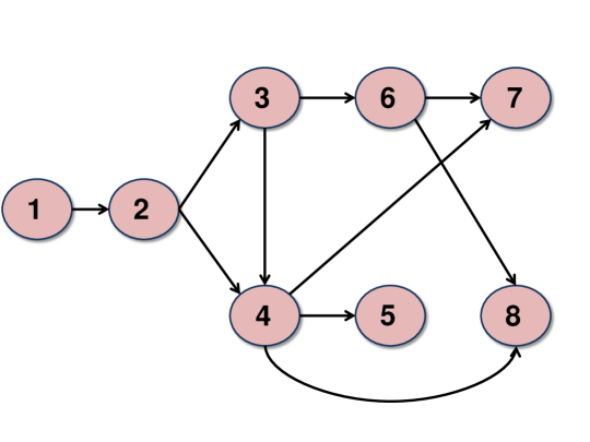
1. Introduction 2. Hypothesis Testing 3. Source Coding 4.  Channel Coding 5.  Channels with State 6.  Slepian-Wolf 7.  Gaussian IC 8.  Gaussian A-MAC

Figure 1.1: Dependence graph of the chapters in this monograph. An arrow from node $s$ to $t$ means that results and techniques in Chapter $s$ are required to understand the material in Chapter $t$.

Part III of this monograph contains a sparse sampling of fixed error asymptotic results in network information theory. The problems we discuss here have conclusive second-order asymptotic characterizations (analogous to the second terms in the asymptotic expansions in (1.3) and (1.4)). They include some channels with random state (Chapter 5), such as Costa’s writing on dirty paper [30], mixed DMCs [67, Sec. 3.3], and quasi-static single-input-multiple-output (SIMO) fading channels [18]. Under the fixed error setup, we also consider the second-order asymptotics of the Slepian-Wolf [151] distributed lossless source coding problem (Chapter 6), the Gaussian interference channel (IC) in the strictly very strong interference regime [22] (Chapter 7), and the Gaussian multiple access channel (MAC) with degraded message sets (Chapter 8). The MAC with degraded message sets is also known as the cognitive [44] or asymmetric [72, 167, 128] MAC (A-MAC). Chapter 9 concludes with a brief summary of other results, together with open problems in this area of research. A dependence graph of the chapters in the monograph is shown in Fig. 1.1.

This area of information theory—fixed error asymptotics—is vast and, at the same time, rapidly expanding. The results described herein are not meant to be exhaustive and were somewhat dependent on the author’s understanding of the subject and his preferences at the time of writing. However, the author has made it a point to ensure that results herein are conclusive in nature. This means that the problem is solved in the information-theoretic sense in that an operational quantity is equated to an information quantity. In terms of asymptotic expansions such as (1.3) and (1.4), by solved, we mean that either the second-order term is known or, better still, both the second- and third-order terms are known. Having articulated this, the author confesses that there are many relevant information-theoretic problems that can be considered solved in the fixed error setting, but have not found their way into this monograph either due to space constraints or because it was difficult to meld them seamlessly with the rest of the story.

1.3 Fundamentals of Information Theory

In this section, we review some basic information-theoretic quantities. As with every article published in the Foundations and Trends in Communications and Information Theory, the reader is expected to have some background in information theory. Nevertheless, the only prerequisite required to appreciate this monograph is information theory at the level of Cover and Thomas [33]. We will also make extensive use of the method of types, for which excellent expositions can be found in [37, 39, 74]. The measure-theoretic foundations of probability will not be needed to keep the exposition accessible to as wide an audience as possible.

1.3.1 Notation

The notation we use is reasonably standard and generally follows the books by Csiszár-Körner [39] and Han [67]. Random variables (e.g., $X$) and their realizations (e.g., $x$) are in upper and lower case respectively. Random variables that take on finitely many values have alphabets (support) that are denoted by calligraphic font (e.g., $\mathcal{X}$). The cardinality of the finite set $\mathcal{X}$ is denoted as $|\mathcal{X}|$. Let the random vector $X^{n}$ be the vector of random variables $(X_{1},\ldots,X_{n})$. We use bold face $\mathbf{x}=(x_{1},\ldots,x_{n})$ to denote a realization of $X^{n}$. The set of all distributions (probability mass functions) supported on alphabet $\mathcal{X}$ is denoted as $\mathscr{P}(\mathcal{X})$. The set of all conditional distributions (i.e., channels) with the input alphabet $\mathcal{X}$ and the output alphabet $\mathcal{Y}$ is denoted by $\mathscr{P}(\mathcal{Y}|\mathcal{X})$. The joint distribution induced by a marginal distribution $P\in\mathscr{P}(\mathcal{X})$ and a channel $V\in\mathscr{P}(\mathcal{Y}|\mathcal{X})$ is denoted as $P\times V$, i.e.,

$$(P\times V)(x,y):=P(x)V(y|x).$$ (1.5)

The marginal output distribution induced by $P$ and $V$ is denoted as $PV$, i.e.,

$$PV(y):=\sum_{x\in\mathcal{X}}P(x)V(y|x).$$ (1.6)

If $X$ has distribution $P$, we sometimes write this as $X\sim P$.

Vectors are indicated in lower case bold face (e.g., $\mathbf{a}$) and matrices in upper case bold face (e.g., $\mathbf{A}$). If we write $\mathbf{a}\geq\mathbf{b}$ for two vectors $\mathbf{a}$ and $\mathbf{b}$ of the same length, we mean that $a_{j}\geq b_{j}$ for every coordinate $j$. The transpose of $\mathbf{A}$ is denoted as $\mathbf{A}^{\prime}$. The vector of all zeros and the identity matrix are denoted as $\mathbf{0}$ and $\mathbf{I}$ respectively. We sometimes make the lengths and sizes explicit. The $\ell_{q}$-norm (for $q\geq 1$) of a vector $\mathbf{v}=(v_{1},\ldots,v_{k})$ is denoted as $\|\mathbf{v}\|_{q}:=(\sum_{i=1}^{k}|v_{i}|^{q})^{1/q}$.

We use standard asymptotic notation [29]: $a_{n}\in O(b_{n})$ if and only if (iff) $\limsup_{n\to\infty}\big{|}a_{n}/b_{n}\big{|}<\infty$; $a_{n}\in\Omega(b_{n})$ iff $b_{n}\in O(a_{n})$; $a_{n}\in\Theta(b_{n})$ iff $a_{n}\in O(b_{n})\cap\Omega(b_{n})$; $a_{n}\in o(b_{n})$ iff $\limsup_{n\to\infty}\big{|}a_{n}/b_{n}\big{|}=0$; and $a_{n}\in\omega(b_{n})$ iff $\liminf_{n\to\infty}\big{|}a_{n}/b_{n}\big{|}=\infty$. Finally, $a_{n}\sim b_{n}$ iff $\lim_{n\to\infty}a_{n}/b_{n}=1$.

1.3.2 Information-Theoretic Quantities

Information-theoretic quantities are denoted in the usual way [39, 49]. All logarithms and exponential functions are to the base $2$. The entropy of a discrete random variable $X$ with probability distribution $P\in\mathscr{P}(\mathcal{X})$ is denoted as

$$H(X)=H(P):=-\sum_{x\in\mathcal{X}}P(x)\log P(x).$$ (1.7)

For the sake of clarity, we will sometimes make the dependence on the distribution $P$ explicit. Similarly given a pair of random variables $(X,Y)$ with joint distribution $P\times V\in\mathscr{P}(\mathcal{X}\times\mathcal{Y})$, the conditional entropy of $Y$ given $X$ is written as

$$H(Y|X)=H(V|P):=-\sum_{x\in\mathcal{X}}P(x)\sum_{y\in\mathcal{Y}}V(y|x)\log V(y|x).$$ (1.8)

The joint entropy is denoted as

$$H(X,Y) :=H(X)+H(Y|X),\quad\mbox{or}$$ (1.9)

$$H(P\times V) :=H(P)+H(V|P).$$ (1.10)

The mutual information is a measure of the correlation or dependence between random variables $X$ and $Y$. It is interchangeably denoted as

$$I(X;Y) :=H(Y)-H(Y|X),\quad\mbox{or}$$ (1.11)

$$I(P,V) :=H(PV)-H(V|P).$$ (1.12)

Given three random variables $(X,Y,Z)$ with joint distribution $P\times V\times W$ where $V\in\mathscr{P}(\mathcal{Y}|\mathcal{X})$ and $W\in\mathscr{P}(\mathcal{Z}|\mathcal{X}\times\mathcal{Y})$, the conditional mutual information is

$$I(Y;Z|X) :=H(Z|X)-H(Z|XY),\quad\mbox{or}$$ (1.13)

$$I(V,W|P) :=\sum_{x\in\mathcal{X}}P(x)I\big{(}V(\cdot|x),W(\cdot|x,\cdot)\big{)}.$$ (1.14)

A particularly important quantity is the relative entropy (or Kullback-Leibler divergence [102]) between $P$ and $Q$ which are distributions on the same finite support set $\mathcal{X}$. It is defined as the expectation with respect to $P$ of the log-likelihood ratio $\log\frac{P(x)}{Q(x)}$, i.e.,

$$D(P\|Q):=\sum_{x\in\mathcal{X}}P(x)\log\frac{P(x)}{Q(x)}.$$ (1.15)

Note that if there exists an $x\in\mathcal{X}$ for which $Q(x)=0$ while $P(x)>0$, then the relative entropy $D(P\|Q)=\infty$. If for every $x\in\mathcal{X}$, if $Q(x)=0$ then $P(x)=0$, we say that $P$ is absolutely continuous with respect to $Q$ and denote this relation by $P\ll Q$. In this case, the relative entropy is finite. It is well known that $D(P\|Q)\geq 0$ and equality holds if and only if $P=Q$. Additionally, the conditional relative entropy between $V,W\in\mathscr{P}(\mathcal{Y}|\mathcal{X})$ given $P\in\mathscr{P}(\mathcal{X})$ is defined as

$$D(V\|W|P):=\sum_{x\in\mathcal{X}}P(x)D\big{(}V(\cdot|x)\|W(\cdot|x)\big{)}.$$ (1.16)

The mutual information is a special case of the relative entropy. In particular, we have

$$I(P,V)=D(P\times V\|P\times PV)=D(V\|PV|P).$$ (1.17)

Furthermore, if $U_{\mathcal{X}}$ is the uniform distribution on $\mathcal{X}$, i.e., $U_{\mathcal{X}}(x)=1/|\mathcal{X}|$ for all $x\in\mathcal{X}$, we have

$$D(P\|U_{\mathcal{X}})=-H(P)+\log|\mathcal{X}|.$$ (1.18)

The definition of relative entropy $D(P\|Q)$ can be extended to the case where $Q$ is not necessarily a probability measure. In this case non-negativity does not hold in general. An important property we exploit is the following: If $\mu$ denotes the counting measure (i.e., $\mu(\mathcal{A})=|\mathcal{A}|$ for $\mathcal{A}\subset\mathcal{X}$), then similarly to (1.18)

$$D(P\|\mu)=-H(P).$$ (1.19)

1.4 The Method of Types

For finite alphabets, a particularly convenient tool in information theory is the method of types [37, 39, 74]. For a sequence $\mathbf{x}=(x_{1},\ldots,x_{n})\in\mathcal{X}^{n}$ in which $|\mathcal{X}|$ is finite, its type or empirical distribution is the probability mass function

$$P_{\mathbf{x}}(x)=\frac{1}{n}\sum_{i=1}^{n}\leavevmode\hbox{\small 1\normalsize\kern-3.30002pt1}\{x_{i}=x\},\qquad\forall\,x\in\mathcal{X}.$$ (1.20)

Throughout, we use the notation $\leavevmode\hbox{\small 1\normalsize\kern-3.30002pt1}\{\mathrm{clause}\}$ to mean the indicator function, i.e., this function equals $1$ if “$\mathrm{clause}$” is true and $0$ otherwise. The set of types formed from $n$-length sequences in $\mathcal{X}$ is denoted as $\mathscr{P}_{n}(\mathcal{X})$. This is clearly a subset of $\mathscr{P}(\mathcal{X})$. The type class of $P$, denoted as $\mathcal{T}_{P}$, is the set of all sequences of length $n$ for which their type is $P$, i.e.,

$$\mathcal{T}_{P}:=\left\{\mathbf{x}\in\mathcal{X}^{n}:P_{\mathbf{x}}=P\right\}.$$ (1.21)

It is customary to indicate the dependence of $\mathcal{T}_{P}$ on the blocklength $n$ but we suppress this dependence for the sake of conciseness throughout. For a sequence $\mathbf{x}\in\mathcal{T}_{P}$, the set of all sequences $\mathbf{y}\in\mathcal{Y}^{n}$ such that $(\mathbf{x},\mathbf{y})$ has joint type $P\times V$ is the $V$-shell, denoted as $\mathcal{T}_{V}(\mathbf{x})$. In other words,

$$\mathcal{T}_{V}(\mathbf{x}):=\left\{\mathbf{y}\in\mathcal{Y}^{n}:P_{\mathbf{x},\mathbf{y}}=P\times V\right\}.$$ (1.22)

The conditional distribution $V$ is also known as the conditional type of $\mathbf{y}$ given $\mathbf{x}$. Let $\mathscr{V}_{n}(\mathcal{Y};P)$ be the set of all $V\in\mathscr{P}(\mathcal{Y}|\mathcal{X})$ for which the $V$-shell of a sequence of type $P$ is non-empty.

We will often times find it useful to consider information-theoretic quantities of empirical distributions. All such quantities are denoted using hats. So for example, the empirical entropy of a sequence $\mathbf{x}\in\mathcal{X}^{n}$ is denoted as

$$\hat{H}(\mathbf{x}):=H(P_{\mathbf{x}}).$$ (1.23)

The empirical conditional entropy of $\mathbf{y}\in\mathcal{Y}^{n}$ given $\mathbf{x}\in\mathcal{X}^{n}$ where $\mathbf{y}\in\mathcal{T}_{V}(\mathbf{x})$ is denoted as

$$\hat{H}(\mathbf{y}|\mathbf{x}):=H(V|P_{\mathbf{x}}).$$ (1.24)

The empirical mutual information of a pair of sequences $(\mathbf{x},\mathbf{y})\in\mathcal{X}^{n}\times\mathcal{Y}^{n}$ with joint type $P_{\mathbf{x},\mathbf{y}}=P_{\mathbf{x}}\times V$ is denoted as

$$\hat{I}(\mathbf{x}\wedge\mathbf{y}):=I(P_{\mathbf{x}},V).$$ (1.25)

The following lemmas form the basis of the method of types. The proofs can be found in [37, 39].

Lemma 1.1 (Type Counting).

The sets $\mathscr{P}_{n}(\mathcal{X})$ and $\mathscr{V}_{n}(\mathcal{Y};P)$ for $P\in\mathscr{P}_{n}(\mathcal{X})$ satisfy

$$|\mathscr{P}_{n}(\mathcal{X})|\leq(n+1)^{|\mathcal{X}|},\quad\mbox{and}\quad|\mathscr{V}_{n}(\mathcal{Y};P)|\leq(n+1)^{|\mathcal{X}||\mathcal{Y}|}.$$ (1.26)

In fact, it is easy to check that $|\mathscr{P}_{n}(\mathcal{X})|=\binom{n+|\mathcal{X}|-1}{|\mathcal{X}|-1}$ but (1.26) or its slightly stronger version

$$|\mathscr{P}_{n}(\mathcal{X})|\leq(n+1)^{|\mathcal{X}|-1}$$ (1.27)

usually suffices for our purposes in this monograph. This key property says that the number of types is polynomial in the blocklength $n$.

Lemma 1.2 (Size of Type Class).

For a type $P\in\mathscr{P}_{n}(\mathcal{X})$, the type class $\mathcal{T}_{P}\subset\mathcal{X}^{n}$ satisfies

$$|\mathscr{P}_{n}(\mathcal{X})|^{-1}\exp\big{(}nH(P)\big{)}\leq|\mathcal{T}_{P}|\leq\exp\big{(}nH(P)\big{)}.$$ (1.28)

For a conditional type $V\in\mathscr{V}_{n}(\mathcal{Y};P)$ and a sequence $\mathbf{x}\in\mathcal{T}_{P}$, the $V$-shell $\mathcal{T}_{V}(\mathbf{x})\subset\mathcal{Y}^{n}$ satisfies

$$|\mathscr{V}_{n}(\mathcal{Y};P)|^{-1}\exp\big{(}nH(V|P)\big{)}\leq|\mathcal{T}_{V}(\mathbf{x})|\leq\exp\big{(}nH(V|P)\big{)}.$$ (1.29)

This lemma says that, on the exponential scale,

$$|\mathcal{T}_{P}|\cong\exp\big{(}nH(P)\big{)},\quad\mbox{and}\quad|\mathcal{T}_{V}(\mathbf{x})|\cong\exp\big{(}nH(V|P)\big{)},$$ (1.30)

where we used the notation $a_{n}\cong b_{n}$ to mean equality up to a polynomial, i.e., there exists polynomials $p_{n}$ and $q_{n}$ such that $a_{n}/p_{n}\leq b_{n}\leq q_{n}a_{n}$. We now consider probabilities of sequences. Throughout, for a distribution $Q\in\mathscr{P}(\mathcal{X})$, we let $Q^{n}(\mathbf{x})$ be the product distribution, i.e.,

$$Q^{n}(\mathbf{x})=\prod_{i=1}^{n}Q(x_{i}),\qquad\forall\,\mathbf{x}\in\mathcal{X}^{n}.$$ (1.31)

Lemma 1.3 (Probability of Sequences).

If $\mathbf{x}\in\mathcal{T}_{P}$ and $\mathbf{y}\in\mathcal{T}_{V}(\mathbf{x})$,

$$Q^{n}(\mathbf{x}) =\exp\big{(}-nD(P\|Q)-nH(P)\big{)}\quad\mbox{and}$$ (1.32)

$$W^{n}(\mathbf{y}|\mathbf{x}) =\exp\big{(}-nD(V\|W|P)-nH(V|P)\big{)}.$$ (1.33)

This, together with Lemma 1.2, leads immediately to the final lemma in this section.

Lemma 1.4 (Probability of Type Classes).

For a type $P\in\mathscr{P}_{n}(\mathcal{X})$,

$$|\mathscr{P}_{n}(\mathcal{X})|^{-1}\exp\big{(}-nD(P\|Q)\big{)}\leq Q^{n}(\mathcal{T}_{P})\leq\exp\big{(}-nD(P\|Q)\big{)}.$$ (1.34)

For a conditional type $V\in\mathscr{V}_{n}(\mathcal{Y};P)$ and a sequence $\mathbf{x}\in\mathcal{T}_{P}$, we have

$$|\mathscr{V}_{n}(\mathcal{Y};P)|^{-1}\exp\big{(}-nD(V\|W|P)\big{)} \leq W^{n}(\mathcal{T}_{V}(\mathbf{x})|\mathbf{x})$$

$$\leq\exp\big{(}-nD(V\|W|P)\big{)}.$$ (1.35)

The interpretation of this lemma is that the probability that a random i.i.d. (independently and identically distributed) sequence $X^{n}$ generated from $Q^{n}$ belongs to the type class $\mathcal{T}_{P}$ is exponentially small with exponent $D(P\|Q)$, i.e.,

$$Q^{n}(\mathcal{T}_{P})\cong\exp\big{(}-nD(P\|Q)\big{)}.$$ (1.36)

The bounds in (1.35) can be interpreted similarly.

1.5 Probability Bounds

In this section, we summarize some bounds on probabilities that we use extensively in the sequel. For a random variable $X$, we let $\mathsf{E}[X]$ and $\operatorname{\mathsf{Var}}(X)$ be its expectation and variance respectively. To emphasize that the expectation is taken with respect to a random variable $X$ with distribution $P$, we sometimes make this explicit by using a subscript, i.e., $\mathsf{E}_{X}$ or $\mathsf{E}_{P}$.

1.5.1 Basic Bounds

We start with the familiar Markov and Chebyshev inequalities.

Proposition 1.1 (Markov’s inequality).

Let $X$ be a real-valued non-negative random variable. Then for any $a>0$, we have

$$\Pr(X\geq a)\leq\frac{\mathsf{E}[X]}{a}.$$ (1.37)

If we let $X$ above be the non-negative random variable $(X-\mathsf{E}[X])^{2}$, we obtain Chebyshev’s inequality.

Proposition 1.2 (Chebyshev’s inequality).

Let $X$ be a real-valued random variable with mean $\mu$ and variance $\sigma^{2}$. Then for any $b>0$, we have

$$\Pr\big{(}|X-\mu|\geq b\sigma\big{)}\leq\frac{1}{b^{2}}.$$ (1.38)

We now consider a collection of real-valued random variables that are i.i.d. In particular, let $X^{n}=(X_{1},\ldots,X_{n})$ be a collection of independent random variables where each $X_{i}$ has distribution $P$ with zero mean and finite variance $\sigma^{2}$.

Proposition 1.3 (Weak Law of Large Numbers).

For every $\epsilon>0$, we have

$$\lim_{n\to\infty}\Pr\left(\bigg{|}\frac{1}{n}\sum_{i=1}^{n}X_{i}\bigg{|}>\epsilon\right)=0.$$ (1.39)

Consequently, the average $\frac{1}{n}\sum_{i=1}^{n}X_{i}$ converges to $0$ in probability.

This follows by applying Chebyshev’s inequality to the random variable $\frac{1}{n}\sum_{i=1}^{n}X_{i}$. In fact, under mild conditions, the convergence to zero in (1.39) occurs exponentially fast. See, for example, Cramer’s theorem in [43, Thm. 2.2.3].

1.5.2 Central Limit-Type Bounds

In preparation for the next result, we denote the probability density function (pdf) of a univariate Gaussian as

$$\mathcal{N}(x;\mu,\sigma^{2})=\frac{1}{\sqrt{2\pi\sigma^{2}}}\mathrm{e}^{-(x-\mu)^{2}/(2\sigma^{2})}.$$ (1.40)

We will also denote this as $\mathcal{N}(\mu,\sigma^{2})$ if the argument $x$ is unnecessary. A standard Gaussian distribution is one in which the mean $\mu=0$ and the standard deviation $\sigma=1$. In the multivariate case, the pdf is

$$\mathcal{N}(\mathbf{x};\bm{\mu},\bm{\Sigma})=\frac{1}{\sqrt{(2\pi)^{k}|\bm{\Sigma}|}}\mathrm{e}^{-\frac{1}{2}(\mathbf{x}-\bm{\mu})^{\prime}\bm{\Sigma}^{-1}(\mathbf{x}-\bm{\mu})}$$ (1.41)

where $\mathbf{x}\in\mathbb{R}^{k}$. A standard multivariate Gaussian distribution is one in which the mean is $\mathbf{0}_{k}$ and the covariance is the identity matrix $\mathbf{I}_{k\times k}$.

For the univariate case, the cumulative distribution function (cdf) of the standard Gaussian is denoted as

$$\Phi(y):=\int_{-\infty}^{y}\mathcal{N}(x;0,1)\,\mathrm{d}x.$$ (1.42)

We also find it convenient to introduce the inverse of $\Phi$ as

$$\Phi^{-1}(\varepsilon):=\sup\big{\{}y\in\mathbb{R}:\Phi(y)\leq\varepsilon\big{\}}$$ (1.43)

which evaluates to the usual inverse for $\varepsilon\in(0,1)$ and extends continuously to take values $\pm\infty$ for $\varepsilon$ outside $(0,1)$. These monotonically increasing functions are shown in Fig. 1.2.

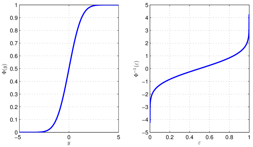
Figure 1.2: Plots of $\Phi(y)$ and $\Phi^{-1}(\varepsilon)$

If the scaling in front of the sum in the statement of the law of large numbers in (1.39) is $\frac{1}{\sqrt{n}}$ instead of $\frac{1}{n}$, the resultant random variable $\frac{1}{\sqrt{n}}\sum_{i=1}^{n}X_{i}$ converges in distribution to a Gaussian random variable. As in Proposition 1.3, let $X^{n}$ be a collection of i.i.d. random variables where each $X_{i}$ has zero mean and finite variance $\sigma^{2}$.

Proposition 1.4 (Central Limit Theorem).

For any $a\in\mathbb{R}$, we have

$$\lim_{n\to\infty}\Pr\left(\frac{1}{\sigma\sqrt{n}}\sum_{i=1}^{n}X_{i}<a\right)=\Phi(a).$$ (1.44)

In other words,

$$\frac{1}{\sigma\sqrt{n}}\sum_{i=1}^{n}X_{i}\stackrel{{\scriptstyle\mathrm{d}}}{{\longrightarrow}}Z$$ (1.45)

where $\stackrel{{\scriptstyle\mathrm{d}}}{{\longrightarrow}}$ means convergence in distribution and $Z$ is the standard Gaussian random variable.

Throughout the monograph, in the evaluation of the non-asymptotic bounds, we will use a more quantitative version of the central limit theorem known as the Berry-Esseen theorem [17, 52]. See Feller [54, Sec. XVI.5] for a proof.

Theorem 1.1 (Berry-Esseen Theorem (i.i.d. Version)).

Assume that the third absolute moment is finite, i.e., $T:=\mathsf{E}\big{[}|X_{1}|^{3}\big{]}<\infty$. For every $n\in\mathbb{N}$, we have

$$\sup_{a\in\mathbb{R}}\left|\Pr\left(\frac{1}{\sigma\sqrt{n}}\sum_{i=1}^{n}X_{i}<a\right)-\Phi(a)\right|\leq\frac{T}{\sigma^{3}\sqrt{n}}.$$ (1.46)

Remarkably, the Berry-Esseen theorem says that the convergence in the central limit theorem in (1.44) is uniform in $a\in\mathbb{R}$. Furthermore, the convergence of the distribution function of $\frac{1}{\sqrt{n}}\sum_{i=1}^{n}X_{i}$ to the Gaussian cdf occurs at a rate of $O(\frac{1}{\sqrt{n}})$. The constant of proportionality in the $O(\cdot)$-notation depends only on the variance and the third absolute moment and not on any other statistics of the random variables.

There are many generalizations of the Berry-Esseen theorem. One which we will need is the relaxation of the assumption that the random variables are identically distributed. Let $X^{n}=(X_{1},\ldots,X_{n})$ be a collection of independent random variables where each random variable has zero mean, variance $\sigma_{i}^{2}:=\mathsf{E}[X_{i}^{2}]>0$ and third absolute moment $T_{i}:=\mathsf{E}\big{[}|X_{i}|^{3}\big{]}<\infty$. We respectively define the average variance and average third absolute moment as

$$\sigma^{2}:=\frac{1}{n}\sum_{i=1}^{n}\sigma_{i}^{2},\quad\mbox{and}\quad T:=\frac{1}{n}\sum_{i=1}^{n}T_{i}.$$ (1.47)

Theorem 1.2 (Berry-Esseen Theorem (General Version)).

For every $n\in\mathbb{N}$, we have

$$\sup_{a\in\mathbb{R}}\left|\Pr\left(\frac{1}{\sigma\sqrt{n}}\sum_{i=1}^{n}X_{i}<a\right)-\Phi(a)\right|\leq\frac{6\,T}{\sigma^{3}\sqrt{n}}.$$ (1.48)

Observe that as with the i.i.d. version of the Berry-Esseen theorem, the remainder term scales as $O(\frac{1}{\sqrt{n}})$.

The proof of the following theorem uses the Berry-Esseen theorem (among other techniques). This theorem is proved in Polyanskiy-Poor-Verdú [123, Lem. 47]. Together with its variants, this theorem is useful for obtaining third-order asymptotics for binary hypothesis testing and other coding problems with non-vanishing error probabilities.

Theorem 1.3.

Assume the same setup as in Theorem 1.2. For any $\gamma\geq 0$, we have

$$\mathsf{E}\left[\exp\bigg{(}-\sum_{i=1}^{n}X_{i}\bigg{)}\leavevmode\hbox{\small 1\normalsize\kern-3.30002pt1}\bigg{\{}\sum_{i=1}^{n}X_{i}>\gamma\bigg{\}}\right]\leq 2\left(\frac{\log 2}{\sqrt{2\pi}}+\frac{12T}{\sigma^{2}}\right)\frac{\exp(-\gamma)}{\sigma\sqrt{n}}.$$ (1.49)

It is trivial to see that the expectation in (1.49) is upper bounded by $\exp(-\gamma)$. The additional factor of $(\sigma\sqrt{n})^{-1}$ is crucial in proving coding theorems with better third-order terms. Readers familiar with strong large deviation theorems or exact asymptotics (see, e.g., [23, Thms. 3.3 and 3.5] or [43, Thm. 3.7.4]) will notice that (1.49) is in the same spirit as the theorem by Bahadur and Ranga-Rao [13]. There are two advantages of (1.49) compared to strong large deviation theorems. First, the bound is purely in terms of $\sigma^{2}$ and $T$, and second, one does not have to differentiate between lattice and non-lattice random variables. The disadvantage of (1.49) is that the constant is worse but this will not concern us as we focus on asymptotic results in this monograph, hence constants do not affect the main results.

For multi-terminal problems that we encounter in the latter parts of this monograph, we will require vector (or multidimensional) versions of the Berry-Esseen theorem. The following is due to Götze [63].

Theorem 1.4 (Vector Berry-Esseen Theorem I).

Let $X_{1}^{k},\ldots,X_{n}^{k}$ be independent $\mathbb{R}^{k}$-valued random vectors with zero mean. Let

$$S_{n}^{k}=\frac{1}{\sqrt{n}}\sum_{i=1}^{n}X_{i}^{k}.$$ (1.50)

Assume that $S_{n}^{k}$ has the following statistics

$$\operatorname{\mathsf{Cov}}(S_{n}^{k})=\mathsf{E}\big{[}S_{n}^{k}(S_{n}^{k})^{\prime}\big{]}=\mathbf{I}_{k\times k},\quad\mbox{and}\quad\xi:=\frac{1}{n}\sum_{i=1}^{n}\mathsf{E}\big{[}\|X_{i}^{k}\|^{3}_{2}\big{]}.$$ (1.51)

Let $Z^{k}$ be a standard Gaussian random vector, i.e., its distribution is $\mathcal{N}(0^{k},\mathbf{I}_{k\times k})$. Then, for all $n\in\mathbb{N}$, we have

$$\sup_{\mathscr{C}\in\mathfrak{C}_{k}}\left|\Pr\big{(}S_{n}^{k}\in\mathscr{C}\big{)}-\Pr\big{(}Z^{k}\in\mathscr{C}\big{)}\right|\leq\frac{c_{k}\,\xi}{\sqrt{n}},$$ (1.52)

where $\mathfrak{C}_{k}$ is the family of all convex subsets of $\mathbb{R}^{k}$, and where $c_{k}$ is a constant that depends only on the dimension $k$.

Theorem 1.4 can be applied for random vectors that are independent but not necessarily identically distributed. The constant $c_{k}$ can be upper bounded by $400\,k^{1/4}$ if the random vectors are i.i.d., a result by Bentkus [15]. However, its precise value will not be of concern to us in this monograph. Observe that the scalar versions of the Berry-Esseen theorems (in Theorems 1.1 and 1.2) are special cases (apart from the constant) of the vector version in which the family of convex subsets is restricted to the family of semi-infinite intervals $(-\infty,a)$.

We will frequently encounter random vectors with non-identity covariance matrices. The following modification of Theorem 1.4 is due to Watanabe-Kuzuoka-Tan [177, Cor. 29].

Corollary 1.1 (Vector Berry-Esseen Theorem II).

Assume the same setup as in Theorem 1.4, except that $\operatorname{\mathsf{Cov}}(S_{n}^{k})=\mathbf{V}$, a positive definite matrix. Then, for all $n\in\mathbb{N}$, we have

$$\sup_{\mathscr{C}\in\mathfrak{C}_{k}}\left|\Pr\big{(}S_{n}^{k}\in\mathscr{C}\big{)}-\Pr\big{(}Z^{k}\in\mathscr{C}\big{)}\right|\leq\frac{c_{k}\,\xi}{\lambda_{\min}(\mathbf{V})^{3/2}\sqrt{n}},$$ (1.53)

where $\lambda_{\min}(\mathbf{V})>0$ is the smallest eigenvalue of $\mathbf{V}$.

The final probability bound is a quantitative version of the so-called multivariate delta method [174, Thm. 5.15]. Numerous similar statements of varying generalities have appeared in the statistics literature (e.g., [24, 175]). The simple version we present was shown by MolavianJazi and Laneman [112] who extended ideas in Hoeffding and Robbins’ paper [81, Thm. 4] to provide rates of convergence to Gaussianity under appropriate technical conditions. This result essentially says that a differentiable function of a normalized sum of independent random vectors also satisfies a Berry-Esseen-type result.

Theorem 1.5 (Berry-Esseen Theorem for Functions of i.i.d. Random Vectors).

Assume that $X_{1}^{k},\ldots,X_{n}^{k}$ are $\mathbb{R}^{k}$-valued, zero-mean, i.i.d. random vectors with positive definite covariance $\operatorname{\mathsf{Cov}}(X_{1}^{k})$ and finite third absolute moment $\xi:=\mathsf{E}[\|X_{1}^{k}\|_{2}^{3}]$. Let $\mathbf{f}(\mathbf{x})$ be a vector-valued function from $\mathbb{R}^{k}$ to $\mathbb{R}^{l}$ that is also twice continuously differentiable in a neighborhood of $\mathbf{x}=\mathbf{0}$. Let $\mathbf{J}\in\mathbb{R}^{l\times k}$ be the Jacobian matrix of $\mathbf{f}(\mathbf{x})$ evaluated at $\mathbf{x}=\mathbf{0}$, i.e., its elements are

$$J_{ij}=\frac{\partial f_{i}(\mathbf{x})}{\partial x_{j}}\bigg{|}_{\mathbf{x}=\mathbf{0}},$$ (1.54)

where $i=1,\ldots,l$ and $j=1,\ldots,k$. Then, for every $n\in\mathbb{N}$, we have

$$\sup_{\mathscr{C}\in\mathfrak{C}_{l}}\left|\Pr\Bigg{(}\mathbf{f}\bigg{(}\frac{1}{n}\sum_{i=1}^{n}X_{i}^{k}\bigg{)}\in\mathscr{C}\Bigg{)}-\Pr\big{(}Z^{l}\in\mathscr{C}\big{)}\right|\leq\frac{c}{\sqrt{n}}$$ (1.55)

where $c>0$ is a finite constant, and $Z^{l}$ is a Gaussian random vector in $\mathbb{R}^{l}$ with mean vector and covariance matrix respectively given as

$$\mathsf{E}[Z^{l}]=\mathbf{f}(\mathbf{0}),\quad\mbox{and}\quad\operatorname{\mathsf{Cov}}(Z^{l})=\frac{\mathbf{J}\operatorname{\mathsf{Cov}}(X^{k}_{1})\mathbf{J}^{\prime}}{n}.$$ (1.56)

In particular, the inequality in (1.55) implies that

$$\sqrt{n}\left(\mathbf{f}\bigg{(}\frac{1}{n}\sum_{i=1}^{n}X_{i}^{k}\bigg{)}-\mathbf{f}(\mathbf{0})\right)\stackrel{{\scriptstyle\mathrm{d}}}{{\longrightarrow}}\mathcal{N}\left(\mathbf{0},\mathbf{J}\operatorname{\mathsf{Cov}}(X^{k}_{1})\mathbf{J}^{\prime}\right),$$ (1.57)

which is a canonical statement in the study of the multivariate delta method [174, Thm. 5.15].

Finally, we remark that Ingber-Wang-Kochman [87] used a result similar to that of Theorem 1.5 to derive second-order asymptotic results for various Shannon-theoretic problems. However, they analyzed the behavior of functions of distributions instead of functions of random vectors as in Theorem 1.5.

Chapter 2 Binary Hypothesis Testing

In this chapter, we review asymptotic expansions in simple (non-composite) binary hypothesis testing when one of the two error probabilities is non-vanishing. We find this useful, as many coding theorems we encounter in subsequent chapters can be stated in terms of quantities related to binary hypothesis testing. For example, as pointed out in Csiszár and Körner [39, Ch. 1], fixed-to-fixed length lossless source coding and binary hypothesis testing are intimately connected through the relation between relative entropy and entropy in (1.18). Another example is in point-to-point channel coding, where a powerful non-asymptotic converse theorem [152, Eq. (4.29)] [123, Sec. III-E] [164, Prop. 6] can be stated in terms of the so-called $\varepsilon$-hypothesis testing divergence and the $\varepsilon$-information spectrum divergence (cf. Proposition 4.4). The properties of these two quantities, as well as the relation between them are discussed. Using various probabilistic limit theorems, we also evaluate these quantities in the asymptotic setting for product distributions. A corollary of the results presented is the familiar Chernoff-Stein lemma [39, Thm. 1.2], which asserts that the exponent with growing number of observations of the type-II error for a non-vanishing type-I error in a binary hypothesis test of $P$ against $Q$ is the relative entropy $D(P\|Q)$.

The material in this chapter is based largely on the seminal work by Strassen [152, Thm. 3.1]. The exposition is based on the more recent works by Polyanskiy-Poor-Verdú [123, App. C], Tomamichel-Tan [164, Sec. III] and Tomamichel-Hayashi [163, Lem. 12].

2.1 Non-Asymptotic Quantities and Their Properties

Consider the simple (non-composite) binary hypothesis test:

$$\mathsf{H}_{0} :Z\sim P$$

$$\mathsf{H}_{1} :Z\sim Q$$ (2.1)

where $P$ and $Q$ are two probability distributions on the same space $\mathcal{Z}$. We assume that the space $\mathcal{Z}$ is finite to keep the subsequent exposition simple. The notation in (2.1) means that under the null hypothesis $\mathsf{H}_{0}$, the random variable $Z$ is distributed as $P\in\mathscr{P}(\mathcal{Z})$ while under the alternative hypothesis $\mathsf{H}_{1}$, it is distributed according to a different distribution $Q\in\mathscr{P}(\mathcal{Z})$. We would like to study the optimal performance of a hypothesis test in terms of the distributions $P$ and $Q$.

There are several ways to measure the performance of a hypothesis test which, in precise terms, is a mapping $\delta$ from the observation space $\mathcal{Z}$ to $[0,1]$. If the observation $z$ is such that $\delta(z)\approx 0$, this means the test favors the null hypothesis $\mathsf{H}_{0}$. Conversely, $\delta(z)\approx 1$ means that the test favors the alternative hypothesis $\mathsf{H}_{1}$ (or alternatively, rejects the null hypothesis $\mathsf{H}_{0}$). If $\delta(z)\in\{0,1\}$, the test is called deterministic, otherwise it is called randomized. Traditionally, there are three quantities that are of interest for a given test $\delta$. The first is the probability of false alarm

$$\mathrm{P}_{\mathrm{FA}}:=\sum_{z\in\mathcal{Z}}\delta(z)P(z)=\mathsf{E}_{P}\big{[}\delta(Z)\big{]}.$$ (2.2)

The second is the probability of missed detection

$$\mathrm{P}_{\mathrm{MD}}:=\sum_{z\in\mathcal{Z}}\big{(}1-\delta(z)\big{)}Q(z)=\mathsf{E}_{Q}\big{[}1-\delta(Z)\big{]}.$$ (2.3)

The third is the probability of detection, which is one minus the probability of missed detection, i.e.,

$$\mathrm{P}_{\mathrm{D}}:=\sum_{z\in\mathcal{Z}}\delta(z)Q(z)=\mathsf{E}_{Q}\big{[}\delta(Z)\big{]}.$$ (2.4)

The probability of false alarm and miss detection are traditionally called the type-I and type-II errors respectively in the statistics literature. The probability of detection and the probability of false alarm are also called the power and the significance level respectively. The “holy grail” is, of course, to design a test such that $\mathrm{P}_{\mathrm{FA}}=0$ while $\mathrm{P}_{\mathrm{D}}=1$ but this is clearly impossible unless $P$ and $Q$ are mutually singular measures.

Since misses are usually more costly than false alarms, let us fix a number $\varepsilon\in(0,1)$ that represents a tolerable probability of false alarm (type-I error). Then define the smallest type-II error in the binary hypothesis test (2.1) with type-I error not exceeding $\varepsilon$, i.e.,

$$\beta_{1-\varepsilon}(P,Q):=\inf_{\delta:\mathcal{Z}\to[0,1]}\Big{\{}\mathsf{E}_{Q}\big{[}1-\delta(Z)\big{]}:\mathsf{E}_{P}\big{[}\delta(Z)\big{]}\leq\varepsilon\Big{\}}.$$ (2.5)

Observe that $\mathsf{E}_{P}\big{[}\delta(Z)\big{]}\leq\varepsilon$ constrains the probability of false alarm to be no greater than $\varepsilon$. Thus, we are searching over all tests $\delta$ satisfying $\mathsf{E}_{P}\big{[}\delta(Z)\big{]}\leq\varepsilon$ such that the probability of missed detection is minimized. Intuitively, $\beta_{1-\varepsilon}(P,Q)$ quantifies, in a non-asymptotic fashion, the performance of an optimal hypothesis test between $P$ and $Q$.

A related quantity is the $\varepsilon$-hypothesis testing divergence

$$D_{\mathrm{h}}^{\varepsilon}(P\|Q):=-\log\frac{\beta_{1-\varepsilon}(P,Q)}{1-\varepsilon}.$$ (2.6)

This is a measure of the distinguishability of $P$ from $Q$. As can be seen from (2.6), $\beta_{1-\varepsilon}(P,Q)$ and $D_{\mathrm{h}}^{\varepsilon}(P\|Q)$ are simple functions of each other. We prefer to express the results in this monograph mostly in terms of $D_{\mathrm{h}}^{\varepsilon}(P\|Q)$ because it shares similar properties with the usual relative entropy $D(P\|Q)$, as is evidenced from the following lemma.

Lemma 2.1 (Properties of $D_{\mathrm{h}}^{\varepsilon}$).

The $\varepsilon$-hypothesis testing divergence satisfies the positive definiteness condition [48, Prop. 3.2], i.e.,

$$D_{\mathrm{h}}^{\varepsilon}(P\|Q)\geq 0.$$ (2.7)

Equality holds if and only if $P=Q$. In addition, it also satisfies the data processing inequality [173, Lem. 1], i.e., for any channel $W$,

$$D_{\mathrm{h}}^{\varepsilon}(PW\|QW)\leq D_{\mathrm{h}}^{\varepsilon}(P\|Q).$$ (2.8)

Figure 2.1: Illustration of the $\varepsilon$-information spectrum divergence $D_{\mathrm{s}}^{\varepsilon}(P\|Q)$ which is the largest point $R^{*}$ for which the probability mass to the left is no larger than $\varepsilon$.

While the $\varepsilon$-hypothesis testing divergence occurs naturally and frequently in coding problems, it is usually hard to analyze directly. Thus, we now introduce an equally important quantity. Define the $\varepsilon$-information spectrum divergence $D_{\mathrm{s}}^{\varepsilon}(P\|Q)$ as

$$D_{\mathrm{s}}^{\varepsilon}(P\|Q):=\sup\bigg{\{}R\in\mathbb{R}:P\bigg{(}\Big{\{}z\in\mathcal{Z}:\log\frac{P(z)}{Q(z)}\leq R\Big{\}}\bigg{)}\leq\varepsilon\bigg{\}}.$$ (2.9)

Just as in information spectrum analysis [67], this quantity places the distribution of the log-likelihood ratio $\log\frac{P(Z)}{Q(Z)}$ (where $Z\sim P$), and not just its expectation, in the most prominent role. See Fig. 2.1 for an interpretation of the definition in (2.9).

As we will see, the $\varepsilon$-information spectrum divergence is intimately related to the $\varepsilon$-hypothesis testing divergence (cf. Lemma 2.4). The former is, however, easier to compute. Note that if $P$ and $Q$ are product measures, then by virtue of the fact that $\log\frac{P(Z)}{Q(Z)}$ is a sum of independent random variables, one can estimate the probability in (2.9) using various probability tail bounds. This we do in the following section.

We now state two useful properties of $D_{\mathrm{s}}^{\varepsilon}(P\|Q)$. The proofs of these lemmas are straightforward and can be found in [164, Sec. III.A].

Lemma 2.2 (Sifting from a convex combination).

Let $P\in\mathscr{P}(\mathcal{Z})$ and $Q=\sum_{k}\alpha_{k}Q_{k}$ be an at most countable convex combination of distributions $Q_{k}\in\mathscr{P}(\mathcal{Z})$ with non-negative weights $\alpha_{k}$ summing to one, i.e., $\sum_{k}\alpha_{k}=1$. Then,

$$D_{\mathrm{s}}^{\varepsilon}(P\|Q)\leq\inf_{k}\bigg{\{}D_{\mathrm{s}}^{\varepsilon}(P\|Q_{k})+\log\frac{1}{\alpha_{k}}\bigg{\}}.$$ (2.10)

In particular, Lemma 2.2 tells us that if there exists some $\gamma>0$ such that $\tilde{Q}(z)\leq\gamma Q(z)$ for all $z\in\mathcal{Z}$ then,

$$D_{\mathrm{s}}^{\varepsilon}(P\|\tilde{Q})\geq D_{\mathrm{s}}^{\varepsilon}(P\|Q)-\log\gamma.$$ (2.11)

Lemma 2.3 (“Symbol-wise” relaxation of $D_{\mathrm{s}}^{\varepsilon}$).

Let $W$ and $V$ be two channels from $\mathcal{X}$ to $\mathcal{Y}$ and let $P\in\mathscr{P}(\mathcal{X})$. Then,

$$D_{\mathrm{s}}^{\varepsilon}(P\times W\|P\times V)\leq\sup_{x\in\mathcal{X}}D_{\mathrm{s}}^{\varepsilon}(W(\cdot|x)\|V(\cdot|x)).$$ (2.12)

One can readily toggle between the $\varepsilon$-hypothesis testing divergence and the $\varepsilon$-information spectrum divergence because they satisfy the bounds in the following lemma. The proof of this lemma mimics that of [163, Lem. 12].

Lemma 2.4 (Relation between divergences).

For every $\varepsilon\in(0,1)$ and every $\eta\in(0,1-\varepsilon)$, we have

$$D_{\mathrm{s}}^{\varepsilon}(P\|Q)-\log\frac{1}{1-\varepsilon} \leq D_{\mathrm{h}}^{\varepsilon}(P\|Q)$$ (2.13)

$$\leq D_{\mathrm{s}}^{\varepsilon+\eta}(P\|Q)+\log\frac{1-\varepsilon}{\eta}.$$ (2.14)

Proof.

The following proof is based on that for [163, Lem. 12]. For the lower bound in (2.13), consider the likelihood ratio test

$$\delta(z):=\leavevmode\hbox{\small 1\normalsize\kern-3.30002pt1}\Big{\{}\log\frac{P(z)}{Q(z)}\leq\gamma\Big{\}},\quad\mbox{where}\quad\gamma:=D_{\mathrm{s}}^{\varepsilon}(P\|Q)-\xi$$ (2.15)

for some small $\xi>0$. This test clearly satisfies $\mathsf{E}_{P}\big{[}\delta(Z)\big{]}\leq\varepsilon$ by the definition of the $\varepsilon$-information spectrum divergence. On the other hand,

$$\mathsf{E}_{Q}\big{[}1-\delta(Z)\big{]}$$

$$=\sum_{z\in\mathcal{Z}}Q(z)\leavevmode\hbox{\small 1\normalsize\kern-3.30002pt1}\Big{\{}\log\frac{P(z)}{Q(z)}>\gamma\Big{\}}$$ (2.16)

$$\leq\sum_{z\in\mathcal{Z}}P(z)\exp(-\gamma)\leavevmode\hbox{\small 1\normalsize\kern-3.30002pt1}\Big{\{}\log\frac{P(z)}{Q(z)}>\gamma\Big{\}}$$ (2.17)

$$\leq\sum_{z\in\mathcal{Z}}P(z)\exp(-\gamma)$$ (2.18)

$$\leq\exp(-\gamma)$$ (2.19)

As a result, by the definition of $D_{\mathrm{h}}^{\varepsilon}(P\|Q)$, we have

$$D_{\mathrm{h}}^{\varepsilon}(P\|Q)\geq\gamma-\log\frac{1}{1-\varepsilon}=D_{\mathrm{s}}^{\varepsilon}(P\|Q)-\xi-\log\frac{1}{1-\varepsilon}.$$ (2.20)

Finally, take $\xi\downarrow 0$ to complete the proof of (2.13).

For the upper bound in (2.14), we may assume $D_{\mathrm{h}}^{\varepsilon}(P\|Q)$ is finite; otherwise there is nothing to prove as $P$ is not absolutely continuous with respect to $Q$ and so $D_{\mathrm{s}}^{\varepsilon+\eta}(P\|Q)$ is infinite. According to the definition of $D_{\mathrm{h}}^{\varepsilon}(P\|Q)$, for any $\gamma\geq 0$, there exists a test $\delta$ satisfying $\mathsf{E}_{P}[\delta(Z)]\leq\varepsilon$ such that

$$(1-\varepsilon)\exp(-D_{\mathrm{h}}^{\varepsilon}(P\|Q))$$

$$\geq\mathsf{E}_{Q}\big{[}1-\delta(Z)\big{]}$$ (2.21)

$$\geq\sum_{z:P(z)\leq\gamma Q(z)}Q(z)\big{(}1-\delta(z)\big{)}$$ (2.22)

$$\geq\frac{1}{\gamma}\sum_{z:P(z)\leq\gamma Q(z)}P(z)\big{(}1-\delta(z)\big{)}$$ (2.23)

$$\geq\frac{1}{\gamma}\bigg{[}\sum_{z}P(z)\big{(}1-\delta(z)\big{)}-\sum_{z:P(z)>\gamma Q(z)}P(z)\bigg{]}$$ (2.24)

$$\geq\frac{1}{\gamma}\bigg{[}1-\varepsilon-P\bigg{(}\Big{\{}z:\frac{P(z)}{Q(z)}>\gamma\Big{\}}\bigg{)}\bigg{]}$$ (2.25)

where (2.25) follows because $\mathsf{E}_{P}\big{[}\delta(Z)\big{]}\leq\varepsilon$. Now fix a small $\xi>0$ and choose

$$\gamma=\exp\big{(}D_{\mathrm{s}}^{\varepsilon+\eta}(P\|Q)+\xi\big{)}.$$ (2.26)

Consequently, from (2.25), we have

$$D_{\mathrm{h}}^{\varepsilon}(P\|Q) \leq D_{\mathrm{s}}^{\varepsilon+\eta}(P\|Q)+\xi$$

$$\quad-\log\bigg{(}1-\frac{P\big{(}\big{\{}z:\log\frac{P(z)}{Q(z)}>D_{\mathrm{s}}^{\varepsilon+\eta}(P\|Q)+\xi\big{\}}\big{)}}{1-\varepsilon}\bigg{)}$$ (2.27)

By the definition of $D_{\mathrm{s}}^{\varepsilon+\eta}(P\|Q)$, the probability within the logarithm is upper bounded by $1-\varepsilon-\eta$. Taking $\xi\downarrow 0$ completes the proof of (2.14) and hence, the lemma. ∎

2.2 Asymptotic Expansions

In this section, we consider the asymptotic expansions of $D_{\mathrm{h}}^{\varepsilon}(P^{(n)}\|Q^{(n)})$ and $D_{\mathrm{s}}^{\varepsilon}(P^{(n)}\|Q^{(n)})$ when $P^{(n)}$ and $Q^{(n)}$ are product distributions, i.e.,

$$P^{(n)}(\mathbf{z}):=\prod_{i=1}^{n}P_{i}(z_{i}),\quad\mbox{and}\quad Q^{(n)}(\mathbf{z})=\prod_{i=1}^{n}Q_{i}(z_{i}),$$ (2.28)

for all $\mathbf{z}=(z_{1},\ldots,z_{n})\in\mathcal{Z}^{n}$. The component distributions $\{(P_{i},Q_{i})\}_{i=1}^{n}$ are not necessarily the same for each $i$. However, we do assume for the sake of simplicity that for each $i$, $P_{i}\ll Q_{i}$ so $D(P_{i}\|Q_{i})<\infty$. Let $V(P\|Q)$ be the variance of the log-likelihood ratio between $P$ and $Q$, i.e.,

$$V(P\|Q):=\sum_{z\in\mathcal{Z}}P(z)\bigg{[}\log\frac{P(z)}{Q(z)}-D(P\|Q)\bigg{]}^{2}.$$ (2.29)

This is also known as the relative entropy variance. Let the third absolute moment of the log-likelihood ratio between $P$ and $Q$ be

$$T(P\|Q):=\sum_{z\in\mathcal{Z}}P(z)\bigg{|}\log\frac{P(z)}{Q(z)}-D(P\|Q)\bigg{|}^{3}.$$ (2.30)

Also define the following quantities:

$$D_{n} :=\frac{1}{n}\sum_{i=1}^{n}D(P_{i}\|Q_{i}),$$ (2.31)

$$V_{n} :=\frac{1}{n}\sum_{i=1}^{n}V(P_{i}\|Q_{i}),\quad\mbox{and}$$ (2.32)

$$T_{n} :=\frac{1}{n}\sum_{i=1}^{n}T(P_{i}\|Q_{i}).$$ (2.33)

The first result in this section is the following:

Proposition 2.1 (Berry-Esseen bounds for $D_{\mathrm{s}}^{\varepsilon}$).

Assume there exists a constant $V_{-}>0$ such that $V_{n}\geq V_{-}$. We have

$$\Phi^{-1}\bigg{(}\varepsilon-\frac{6\,T_{n}}{\sqrt{nV_{-}^{3}}}\bigg{)} \leq\frac{D_{\mathrm{s}}^{\varepsilon}(P^{(n)}\|Q^{(n)})-nD_{n}}{\sqrt{nV_{n}}}\leq\Phi^{-1}\bigg{(}\varepsilon+\frac{6\,T_{n}}{\sqrt{nV_{-}^{3}}}\bigg{)}.$$ (2.34)

Proof.

Let $Z^{n}$ be distributed according to $P^{(n)}$. By using the product structure of $P^{(n)}$ and $Q^{(n)}$ in (2.28),

$$\Pr\bigg{(}\log\frac{P^{(n)}(Z^{n})}{Q^{(n)}(Z^{n})}\leq R\bigg{)}=\Pr\bigg{(}\sum_{i=1}^{n}\log\frac{P_{i}(Z_{i})}{Q_{i}(Z_{i})}\leq R\bigg{)}.$$ (2.35)

By the Berry-Esseen theorem in Theorem 1.2, we have

$$\bigg{|}\Pr\bigg{(}\sum_{i=1}^{n}\log\frac{P_{i}(Z_{i})}{Q_{i}(Z_{i})}\leq R\bigg{)}-\Phi\bigg{(}\frac{R-nD_{n}}{\sqrt{nV_{n}}}\bigg{)}\bigg{|}\leq\frac{6\,T_{n}}{\sqrt{nV_{n}^{3}}}.$$ (2.36)

The result immediately follows by using the bound $V_{n}\geq V_{-}$. ∎

A special case of the bound above occurs when $P_{i}=P$ and $Q_{i}=Q$ for all $i=1,\ldots,n$. In this case, we write $P^{n}$ for $P^{(n)}$ and similarly, $Q^{n}$ for $Q^{(n)}$. One has:

Corollary 2.1 (Asymptotics of $D_{\mathrm{s}}^{\varepsilon}$).

If $V(P\|Q)>0$, then

$$D_{\mathrm{s}}^{\varepsilon}(P^{n}\|Q^{n})=nD(P\|Q)+\sqrt{nV(P\|Q)}\Phi^{-1}(\varepsilon)+O(1).$$ (2.37)

Proof.

Since $V(P\|Q)>0$ and $T(P\|Q)<\infty$ (because $P\ll Q$), the term $6\,T_{n}/\sqrt{nV_{-}^{3}}$ in (2.34) is equal to $\frac{c}{\sqrt{n}}$ for some finite $c>0$. By Taylor expansions,

$$\Phi^{-1}\bigg{(}\varepsilon\pm\frac{c}{\sqrt{n}}\bigg{)}=\Phi^{-1}(\varepsilon)+O\bigg{(}\frac{1}{\sqrt{n}}\bigg{)},$$ (2.38)

which completes the proof. ∎

In some applications, it is not possible to guarantee that $V_{n}$ is uniformly bounded away from zero (per Proposition 2.1). In this case, to obtain an upper bound on $D_{\mathrm{s}}^{\varepsilon}$, we employ Chebyshev’s inequality instead of the Berry-Esseen theorem. In the following proposition, which is usually good enough to establish strong converses, we do not assume that the component distributions are the same.

Proposition 2.2 (Chebyshev bound for $D_{\mathrm{s}}^{\varepsilon}$).

We have

$$D_{\mathrm{s}}^{\varepsilon}(P^{(n)}\|Q^{(n)})\leq nD_{n}+\sqrt{\frac{nV_{n}}{1-\varepsilon}}.$$ (2.39)

Proof.

By the definition of the $\varepsilon$-information spectrum divergence, we have

$$D_{\mathrm{s}}^{\varepsilon}(P^{(n)}\|Q^{(n)})=\max\big{\{}D^{-},D^{+}\big{\}}$$ (2.40)

where $D^{-}$ and $D^{+}$ are defined as

$$D^{-} :=\sup\bigg{\{}R\leq nD_{n}:P\bigg{(}\Big{\{}z\in\mathcal{Z}:\log\frac{P(z)}{Q(z)}\leq R\Big{\}}\bigg{)}\leq\varepsilon\bigg{\}},$$ (2.41)

$$D^{+} :=\sup\bigg{\{}R>nD_{n}:P\bigg{(}\Big{\{}z\in\mathcal{Z}:\log\frac{P(z)}{Q(z)}\leq R\Big{\}}\bigg{)}\leq\varepsilon\bigg{\}}.$$ (2.42)

Clearly, $D^{-}\leq nD_{n}$ so it remains to upper bound $D^{+}$. Let $R>nD_{n}$ be fixed. By Chebyshev’s inequality,

$$\Pr\bigg{(}\sum_{i=1}^{n}\log\frac{P_{i}(Z_{i})}{Q_{i}(Z_{i})}\leq R\bigg{)}\geq 1-\frac{nV_{n}}{(R-nD_{n})^{2}}.$$ (2.43)

Hence, we have

$$D^{+} \leq\sup\left\{R>nD_{n}:1-\frac{nV_{n}}{(R-nD_{n})^{2}}\leq\varepsilon\right\}$$ (2.44)

$$=nD_{n}+\sqrt{\frac{nV_{n}}{1-\varepsilon}}.$$ (2.45)

Thus, we see that the bound on $D^{+}$ dominates. This yields (2.39) as desired. ∎

Now we would like an expansion for $D_{\mathrm{h}}^{\varepsilon}$ similar to that for $D_{\mathrm{s}}^{\varepsilon}$ in Corollary 2.1. The following was shown by Strassen [152, Thm. 3.1].

Proposition 2.3 (Asymptotics of $D_{\mathrm{h}}^{\varepsilon}$).

Assume the conditions in Corollary 2.1. The following holds:

$$D_{\mathrm{h}}^{\varepsilon}(P^{n}\|Q^{n})=nD(P\|Q)+\sqrt{nV(P\|Q)}\Phi^{-1}(\varepsilon)+\frac{1}{2}\log n+O(1).$$ (2.46)

As a result, in the asymptotic setting for identical product distributions, $D_{\mathrm{h}}^{\varepsilon}(P^{n}\|Q^{n})$ exceeds $D_{\mathrm{s}}^{\varepsilon}(P^{n}\|Q^{n})$ by $\frac{1}{2}\log n$ ignoring constant terms, i.e.,

$$D_{\mathrm{h}}^{\varepsilon}(P^{n}\|Q^{n})=D_{\mathrm{s}}^{\varepsilon}(P^{n}\|Q^{n})+\frac{1}{2}\log n+O(1).$$ (2.47)

Proof.

Let us first verify the upper bound. Let $\eta$ in the upper bound of Lemma 2.4 be chosen to be $\frac{1}{\sqrt{n}}$. Now, for $n$ large enough (so $\frac{1}{\sqrt{n}}<1-\varepsilon$), combine this upper bound with Corollary 2.1 to obtain that

$$D_{\mathrm{h}}^{\varepsilon}(P^{n}\|Q^{n})\leq D_{\mathrm{s}}^{\varepsilon+\frac{1}{\sqrt{n}}}(P^{n}\|Q^{n})+\frac{1}{2}\log n+\log(1-\varepsilon)$$ (2.48)

$$=nD(P\|Q)+\sqrt{nV(P\|Q)}\Phi^{-1}\bigg{(}\varepsilon+\frac{1}{\sqrt{n}}\bigg{)}+\frac{1}{2}\log n+O(1)$$ (2.49)

Applying a Taylor expansion to the last step and noting that $V(P\|Q)<\infty$ because $P\ll Q$ yields the upper bound in (2.46).

The proof of the lower bound in (2.46) is slightly more involved. Observe that if we naïvely employed (2.13) to lower bound $D_{\mathrm{h}}^{\varepsilon}(P^{n}\|Q^{n})$ with $D_{\mathrm{s}}^{\varepsilon}(P^{n}\|Q^{n})-\log\frac{1}{1-\varepsilon}$, the third-order term would be $O(1)$ instead of the better $\frac{1}{2}\log n+O(1)$. The idea is to propose an appropriate test for $D_{\mathrm{h}}^{\varepsilon}$ and to use Theorem 1.3. Consider the likelihood ratio test

$$\delta(\mathbf{z}):=\leavevmode\hbox{\small 1\normalsize\kern-3.30002pt1}\bigg{\{}\log\frac{P^{n}(\mathbf{z})}{Q^{n}(\mathbf{z})}\leq\gamma\bigg{\}}$$ (2.50)

Define $\sigma^{2}:=V(P\|Q)$ and $T:=T(P\|Q)$. Also define the i.i.d. random variables $U_{i}:=\log P(Z_{i})-\log Q(Z_{i})$, $1\leq i\leq n$, each having variance $\sigma^{2}$ and third absolute moment $T$. Consider, the expectation of $1-\delta(Z^{n})$ under the distribution $Q^{n}$:

$$\mathsf{E}_{Q^{n}}\big{[}1-\delta(Z^{n})\big{]}$$

$$=\sum_{\mathbf{z}}Q^{n}(\mathbf{z})\leavevmode\hbox{\small 1\normalsize\kern-3.30002pt1}\bigg{\{}\log\frac{P^{n}(\mathbf{z})}{Q^{n}(\mathbf{z})}>\gamma\bigg{\}}$$ (2.51)

$$=\sum_{\mathbf{z}}P^{n}(\mathbf{z})\exp\bigg{(}-\log\frac{P^{n}(\mathbf{z})}{Q^{n}(\mathbf{z})}\bigg{)}\leavevmode\hbox{\small 1\normalsize\kern-3.30002pt1}\bigg{\{}\log\frac{P^{n}(\mathbf{z})}{Q^{n}(\mathbf{z})}>\gamma\bigg{\}}$$ (2.52)

$$=\mathsf{E}_{P^{n}}\bigg{[}\exp\bigg{(}-\sum_{i=1}^{n}U_{i}\bigg{)}\leavevmode\hbox{\small 1\normalsize\kern-3.30002pt1}\bigg{\{}\sum_{i=1}^{n}U_{i}>\gamma\bigg{\}}\bigg{]}$$ (2.53)

$$\leq 2\bigg{(}\frac{\log 2}{\sqrt{2\pi}}+\frac{12\,T}{\sigma^{2}}\bigg{)}\frac{\exp(-\gamma)}{\sigma\sqrt{n}}$$ (2.54)

where (2.54) is an application of Theorem 1.3. Now put

$$\gamma:=nD(P\|Q)+\sqrt{nV(P\|Q)}\Phi^{-1}\bigg{(}\varepsilon-\frac{6\,T(P\|Q)}{\sqrt{nV(P\|Q)^{3}}}\bigg{)}.$$ (2.55)

An application of the Berry-Esseen theorem yields

$$\mathsf{E}_{P}\big{[}\delta(Z^{n})\big{]}=P\bigg{(}\Big{\{}\mathbf{z}:\sum_{i=1}^{n}\log\frac{P(z_{i})}{Q(z_{i})}\leq\gamma\Big{\}}\bigg{)}\leq\varepsilon.$$ (2.56)

From (2.54), (2.56) and the definition of $D_{\mathrm{h}}^{\varepsilon}$, we have

$$D_{\mathrm{h}}^{\varepsilon}(P^{n}\|Q^{n}) \geq\gamma+\log\big{(}\sigma\sqrt{n}\big{)}+O(1)=\gamma+\frac{1}{2}\log n+O(1).$$ (2.57)

The proof is concluded by plugging (2.55) into (2.57) and Taylor expanding $\Phi^{-1}(\cdot)$ around $\varepsilon$. ∎

We remark that the lower bound in Proposition 2.3 can be achieved using deterministic tests, i.e., $\delta$ can be chosen to be an indicator function as in (2.50). Randomization is thus unnecessary. Also, one can relax the assumption that $Q^{n}$ is a product probability measure; it can be an arbitrary product measure. These realizations are important to make the connection between hypothesis testing and lossless source coding which we discuss in the next chapter.

A corollary of Proposition 2.3 is the Chernoff-Stein lemma [25] quantifying the error exponent of the probability of missed detection keeping the probability of false alarm bounded above by $\varepsilon$.

Corollary 2.2 (Chernoff-Stein lemma).

Assume the conditions in Corollary 2.1 and recall the definition of $\beta_{1-\varepsilon}$ in (2.5). For every $\varepsilon\in(0,1)$,

$$\lim_{n\to\infty}\frac{1}{n}\log\frac{1}{\beta_{1-\varepsilon}(P^{n},Q^{n})}=\lim_{n\to\infty}\frac{D_{\mathrm{h}}^{\varepsilon}(P^{n}\|Q^{n})}{n}=D(P\|Q).$$ (2.58)

Part II Point-To-Point Communication

Chapter 3 Source Coding

In this chapter, we revisit the fundamental problem of fixed-to-fixed length lossless and lossy source compression. Shannon, in his original paper [141] that launched the field of information theory, showed that the fundamental limit of compression of a discrete memoryless source (DMS) $P$ is the entropy $H(P)$. For the case of continuous sources, lossless compression is not possible and some distortion must be allowed. Shannon showed in [144] that the corresponding fundamental limit of compression of memoryless source $P$ up to distortion $\Delta\geq 0$, assuming a separable distortion measure $d$, is the rate-distortion function

$$R(P,\Delta):=\min_{W\in\mathscr{P}(\hat{\mathcal{X}}|\mathcal{X}):\mathsf{E}_{P\times W}[d(X,\hat{X})]\leq\Delta}I(P,W).$$ (3.1)

These first-order fundamental limits are attained as the number of realizations of the source (i.e., the blocklength of the source) $P$ tends to infinity. The strong converse for rate-distortion is also known and shown, for example, in [39, Ch. 7]. In the following, we present known non-asymptotic bounds for lossless and lossy source coding. We then fix the permissible error probability in the lossless case and the excess distortion probability in the lossy case at some non-vanishing $\varepsilon\in(0,1)$. The non-asymptotic bounds are evaluated as $n$ becomes large so as to obtain asymptotic expansions of the logarithm of the smallest achievable code size. These refined results provide an approximation of the extra code rate (beyond $H(P)$ or $R(P,\Delta)$) one must incur when operating in the finite blocklength regime. Finally, for both the lossless and lossy compression problems, we provide alternative proof techniques based on the method of types that are partially universal.

The material in this chapter concerning lossless source coding is based on the seminal work by Strassen [152, Thm. 1.1]. The material on lossy source coding is based on more recent work by Ingber-Kochman [86] and Kostina-Verdú [97].

3.1 Lossless Source Coding: Non-Asymptotic Bounds

We now set up the almost lossless source coding problem formally. As mentioned, we only consider fixed-to-fixed length source coding in this monograph. A source is simply a probability mass function $P$ on some finite alphabet $\mathcal{X}$ or the associated random variable $X$ with distribution $P$. See Fig. 3.1 for an illustration of the setup.

Figure 3.1: Illustration of the fixed-to-fixed length source coding problem.

An $(M,\varepsilon)$-code for the source $P\in\mathscr{P}(\mathcal{X})$ consists of a pair of maps that includes an encoder $f:\mathcal{X}\to\{1,\ldots,M\}$ and a decoder $\varphi:\{1,\ldots,M\}\to\mathcal{X}$ such that the error probability

$$P\big{(}\{x\in\mathcal{X}:\varphi(f(x))\neq x\}\big{)}\leq\varepsilon.$$ (3.2)

The number $M$ is called the size of the code $(f,\varphi)$.

Given a source $P$, we define the almost lossless source coding non-asymptotic fundamental limit as

$$M^{*}(P,\varepsilon):=\min\big{\{}M\in\mathbb{N}\,:\,\exists\mbox{ an }(M,\varepsilon)\mbox{-code for }P\big{\}}.$$ (3.3)

Obviously for an arbitrary source, the exact evaluation of the minimum code size $M^{*}(P,\varepsilon)$ is challenging. In the following, we assume that it is a discrete memoryless source (DMS), i.e., the distribution $P^{n}$ consists of $n$ copies of an underlying distribution $P$. With this assumption, we can find an asymptotic expansion of $\log M^{*}(P^{n},\varepsilon)$.

The agenda for this and subsequent chapters will largely be standard. We first establish “good” bounds on non-asymptotic quantities like $M^{*}(P,\varepsilon)$. Subsequently, we replace the source or channel with $n$ independent copies of it. Finally, we use an appropriate limit theorem (e.g., those in Section 1.5) to evaluate the non-asymptotic bounds in the large $n$ limit.

3.1.1 An Achievability Bound

One of the take-home messages that we would like to convey in this section is that fixed-to-fixed length lossless source coding is nothing but binary hypothesis testing where the measures $P$ and $Q$ are chosen appropriately. In fact, a reasonable coding scheme for the lossless source coding would simply be to encode a “typical” set of source symbols $\mathcal{T}\subset\mathcal{X}$, ignore the rest, and declare an error if the realized symbol from the source is not in $\mathcal{T}$. In this way, one sees that

$$M^{*}(P,\varepsilon)\leq\min_{\mathcal{T}\subset\mathcal{X}:P(\mathcal{X}\setminus\mathcal{T})\leq\varepsilon}|\mathcal{T}|$$ (3.4)

This bound can be stated in terms of $\beta_{1-\varepsilon}(P,Q)$ or, equivalently, the $\varepsilon$-hypothesis testing divergence $D_{\mathrm{h}}^{\varepsilon}(P\|Q)$ if we restrict the tests that define these quantities to be deterministic, and also allow $Q$ to be an arbitrary measure (not necessarily a probability measure). Let $\mu$ be the counting measure, i.e.,

$$\mu(\mathcal{A}):=|\mathcal{A}|,\quad\forall\,\mathcal{A}\subset\mathcal{X}.$$ (3.5)

Proposition 3.1 (Source coding as hypothesis testing: Achievability).

Let $\varepsilon\in(0,1)$ and $P$ be any source with countable alphabet $\mathcal{X}$. We have

$$M^{*}(P,\varepsilon)\leq\beta_{1-\varepsilon}(P,\mu),$$ (3.6)

or in terms of the $\varepsilon$-hypothesis testing divergence (cf. (2.6)),

$$\log M^{*}(P,\varepsilon)\leq-D_{\mathrm{h}}^{\varepsilon}(P\|\mu)-\log\frac{1}{1-\varepsilon}.$$ (3.7)

3.1.2 A Converse Bound

The converse bound we evaluate is also intimately connected to a divergence we introduced in the previous chapter, namely the $\varepsilon$-information spectrum divergence where the distribution in the alternate hypothesis $Q$ is chosen to be the counting measure.

Proposition 3.2 (Source coding as hypothesis testing: Converse).

Let $\varepsilon\in(0,1)$ and $P$ be any source with countable alphabet $\mathcal{X}$. For any $\eta\in(0,1-\varepsilon)$, we have

$$\log M^{*}(P,\varepsilon)\geq-D_{\mathrm{s}}^{\varepsilon+\eta}(P\|\mu)-\log\frac{1}{\eta}.$$ (3.8)

This statement is exactly Lemma 1.3.2 in Han’s book [67]. Since the proof is short, we provide it for completeness.

Proof.

By the definition of the $\varepsilon$-information spectrum divergence, it is enough to establish that every $(M,\varepsilon)$-code for $P$ must satisfy

$$\varepsilon+\eta\geq P\bigg{(}\Big{\{}x:P(x)\leq\frac{\eta}{M}\Big{\}}\bigg{)},$$ (3.9)

for any $\eta\in(0,1-\varepsilon)$. Let $\mathcal{T}:=\{x:P(x)\leq\frac{\eta}{M}\}$ and let $\mathcal{S}:=\{x:\varphi(f(x))=x\}$. Clearly, $|\mathcal{S}|\leq M$. We have

$$P(\mathcal{T})\leq P(\mathcal{X}\setminus\mathcal{S})+P(\mathcal{T}\cap\mathcal{S})\leq\varepsilon+P(\mathcal{T}\cap\mathcal{S}).$$ (3.10)

Furthermore,

$$P(\mathcal{T}\cap\mathcal{S})=\sum_{x\in\mathcal{T}\cap\mathcal{S}}P(x)\leq\sum_{x\in\mathcal{T}\cap\mathcal{S}}\frac{\eta}{M}\leq|\mathcal{S}|\frac{\eta}{M}\leq\eta.$$ (3.11)

Uniting (3.10) and (3.11) gives (3.9) as desired. ∎

Observe the similarity of this proof to proof of the upper bound of $D_{\mathrm{h}}^{\varepsilon}$ in terms of $D_{\mathrm{s}}^{\varepsilon}$ in Lemma 2.4.

3.2 Lossless Source Coding: Asymptotic Expansions

Now we assume that the source $P^{n}$ is stationary and memoryless, i.e., a DMS. More precisely,

$$P^{n}(\mathbf{x})=\prod_{i=1}^{n}P(x_{i}),\quad\,\forall\,\mathbf{x}\in\mathcal{X}^{n}.$$ (3.12)

We assume throughout that $P(x)>0$ for all $x\in\mathcal{X}$. Shannon [141] showed that the minimum rate to achieve almost lossless compression of a DMS $P$ is the entropy $H(P)$. In this section as well as the next one, we derive finer evaluations of the fundamental compression limit by considering the asymptotic expansion of $\log M^{*}(P^{n},\varepsilon)$. To do so, we need to define another important quantity related to the source $P$.

Let the source dispersion of $P$ be the variance of the self-information random variable $-\log{P(X)}$, i.e.,

$$V(P):=\operatorname{\mathsf{Var}}\bigg{[}\log\frac{1}{P(X)}\bigg{]}=\sum_{x\in\mathcal{X}}P(x)\bigg{[}\log\frac{1}{P(x)}-H(P)\bigg{]}^{2}.$$ (3.13)

Note that the expectation of the self-information is the entropy $H(P)$. In Kontoyannis-Verdú [95], $V(P)$ is called the varentropy. If $V(P)=0$ this means that the source is either deterministic or uniform.

The two non-asymptotic theorems in the preceding section combine to give the following asymptotic expansion of the minimum code size $M^{*}(P^{n},\varepsilon)$.

Theorem 3.1.

If the source $P\in\mathscr{P}(\mathcal{X})$ satisfies $V(P)>0$, then

$$\log M^{*}(P^{n},\varepsilon)=nH(P)-\sqrt{nV(P)}\Phi^{-1}(\varepsilon)-\frac{1}{2}\log n+O(1).$$ (3.14)

Otherwise, we have

$$\log M^{*}(P^{n},\varepsilon)=nH(P)+O(1).$$ (3.15)

Proof.

For the direct part of (3.14) (upper bound), note that the term $-\log\frac{1}{1-\varepsilon}$ in Proposition 3.1 is a constant, so we simply have to evaluate $D_{\mathrm{h}}^{\varepsilon}(P^{n}\|\mu^{n})$. From Corollary 2.1 and its remark that the lower bound on $D_{\mathrm{h}}^{\varepsilon}(P^{n}\|Q^{n})$ can be achieved using deterministic tests, we have

$$D_{\mathrm{h}}^{\varepsilon}(P^{n}\|\mu^{n})=nD(P\|\mu)+\sqrt{nV(P\|\mu)}\Phi^{-1}(\varepsilon)+\frac{1}{2}\log n+O(1).$$ (3.16)

It can easily be verified (cf. (1.19)) that

$$D(P\|\mu)=-H(P),\quad\mbox{and}\quad V(P\|\mu)=V(P).$$ (3.17)

This concludes the proof of the direct part in light of Proposition 3.1.

For the converse part of (3.14) (lower bound), choose $\eta=\frac{1}{\sqrt{n}}$ so the term $-\log\frac{1}{\eta}$ in Proposition 3.2 gives us the $-\frac{1}{2}\log n$ term. Furthermore, by Proposition 2.1 and the simplifications in (3.17),

$$D_{\mathrm{s}}^{\varepsilon+\frac{1}{\sqrt{n}}}(P^{n}\|\mu^{n})=-nH(P)+\sqrt{nV(P)}\Phi^{-1}\bigg{(}\varepsilon+\frac{1}{\sqrt{n}}\bigg{)}+O(1).$$ (3.18)

A Taylor expansion of $\Phi^{-1}(\cdot)$ completes the proof of (3.14).

For (3.15), note that the self-information $-\log P(X)$ takes on the value $H(P)$ with probability one. In other words,

$$P^{n}\big{(}\log P^{n}(X^{n})\leq R\big{)}=\leavevmode\hbox{\small 1\normalsize\kern-3.30002pt1}\big{\{}R\geq-nH(P)\big{\}}.$$ (3.19)

The bounds on $\log M^{*}(P^{n},\varepsilon)$ in Propositions 3.1 and 3.2 and the relaxation to the $\varepsilon$-information spectrum divergence (Lemma 2.4) yields (3.15). ∎

The expansion in (3.14) in Theorem 3.1 appeared in early works by Yushkevich [190] (with $o(\sqrt{n})$ in place of $-\frac{1}{2}\log n$ but for Markov chains) and Strassen [152, Thm. 1.1] (in the form stated). It has since appeared in various other forms and levels of generality in Kontoyannis [93], Hayashi [75], Kostina-Verdú [97], Nomura-Han [117] and Kontoyannis-Verdú [95] among others.

As can be seen from the non-asymptotic bounds and the asymptotic evaluation, fixed-to-fixed length lossless source coding and binary hypothesis testing are virtually the same problem. Asymptotic expansions for $D_{\mathrm{h}}^{\varepsilon}$ and $D_{\mathrm{s}}^{\varepsilon}$ can be used directly to estimate the minimum code size $M^{*}(P^{n},\varepsilon)$ for an $\varepsilon$-reliable lossless source code.

3.3 Second-Order Asymptotics of Lossless Source Coding via the Method of Types

Clearly, the coding scheme described in (3.4) is non-universal, i.e., the code depends on knowledge of the source distribution. In many applications, the exact source distribution is unknown, and hence has to be estimated a priori, or one has to design a source code that works well for any source distribution. It is a well-known application of the method of types that universal source codes achieve the lossless source coding error exponent [39, Thm. 2.15]. One then wonders whether there is any degradation in the asymptotic expansion of $\log M^{*}(P^{n},\varepsilon)$ if the encoder and decoder know less about the source. It turns out that the source dispersion term can be achieved only with the knowledge of $H(P)$ and $V(P)$. However, one has to work much harder to determine the third-order term. For conclusive results on the third-order term for fixed-to-variable length source coding, the reader is referred to the elegant work by Kosut and Sankar [100, 101]. The technique outlined in this section involves the method of types.

Let $M_{\mathrm{u}}^{*}(P,\varepsilon)$ be the almost lossless source coding non-asymptotic fundamental limit where the source code $(f,\varphi)$ is ignorant of the probability distribution of the source $P$, except for the entropy $H(P)$ and the varentropy $V(P)$.

Theorem 3.2.

If the source $P\in\mathscr{P}(\mathcal{X})$ satisfies $V(P)>0$, then

$$\log M_{\mathrm{u}}^{*}(P^{n},\varepsilon)\leq nH(P)-\sqrt{nV(P)}\Phi^{-1}(\varepsilon)+(|\mathcal{X}|-1)\log n+O(1).$$ (3.20)

The proof we present here results in a third-order term that is likely to be far from optimal but we present this proof to demonstrate the similarity to the classical proof of the fixed-to-fixed length source coding error exponent using the method of types [39, Thm. 2.15].

Proof of Theorem 3.2.

Let $\mathcal{X}=\{a_{1},\ldots,a_{d}\}$ without loss of generality. Set $M$, the size of the code, to be the smallest integer exceeding

$$\exp\bigg{[}nH(P) -\sqrt{nV(P)}\Phi^{-1}\Big{(}\varepsilon-\frac{c}{\sqrt{n}}\Big{)}+(d-1)\log(n+1)\bigg{]},$$ (3.21)

for some finite constant $c>0$ (given in Theorem 1.5). Let $\mathcal{K}$ be the set of sequences in $\mathcal{X}^{n}$ whose empirical entropy is no larger than

$$\gamma:=\frac{1}{n}\log M-\frac{(d-1)\log(n+1)}{n}.$$ (3.22)

In other words,

$$\mathcal{K}:=\bigcup_{Q\in\mathscr{P}_{n}(\mathcal{X}):H(Q)\leq\gamma}\mathcal{T}_{Q}.$$ (3.23)

Encode all sequences in $\mathcal{K}$ in a one-to-one way and sequences not in $\mathcal{K}$ arbitrarily. By the type counting lemma in (1.27) and Lemma 1.2 (size of type class), we have

$$|\mathcal{K}|\!\leq\!\sum_{Q\in\mathscr{P}_{n}(\mathcal{X}):H(Q)\leq\gamma}\!\exp\big{(}nH(Q)\big{)}\leq(n+1)^{d-1}\exp\big{(}n\gamma\big{)}\leq M$$ (3.24)

so the number of sequences that can be reconstructed without error is at most $M$ as required. An error occurs if and only if the source sequence has empirical entropy exceeding $\gamma$, i.e., the error probability is

$$\mathfrak{p}:=\Pr(H(P_{X^{n}})>\gamma)$$ (3.25)

where $P_{X^{n}}\in\mathscr{P}_{n}(\mathcal{X})$ is the random type of $X^{n}\in\mathcal{X}^{n}$. This probability can be written as

$$\mathfrak{p}=\Pr\big{(}f(P_{X^{n}}-P)>\gamma\big{)},$$ (3.26)

where the function $f:\mathbb{R}^{d}\to\mathbb{R}$ is defined as

$$f(\mathbf{v})=H\left({\mathbf{v}}+P\right),$$ (3.27)

In (3.26) and (3.27), we regarded the type $P_{X^{n}}$ and the true distribution $P$ as vectors of length $d=|\mathcal{X}|$, and $H(\mathbf{w})=-\sum_{j}w_{j}\log w_{j}$ is the entropy. Note that the argument of $f(\cdot)$ in (3.26) can be written as

$$P_{X^{n}}-P=\frac{1}{{n}}\sum_{i=1}^{n}\begin{bmatrix}\leavevmode\hbox{\small 1\normalsize\kern-3.30002pt1}\{X_{i}=a_{1}\}-P(a_{1})\\ \vdots\\ \leavevmode\hbox{\small 1\normalsize\kern-3.30002pt1}\{X_{i}=a_{d}\}-P(a_{d})\end{bmatrix}=:\frac{1}{n}\sum_{i=1}^{n}U_{i}^{d}.$$ (3.28)

Since $U_{i}^{d}:=[\leavevmode\hbox{\small 1\normalsize\kern-3.30002pt1}\{X_{i}=a_{1}\}-P(a_{1}),\ldots,\leavevmode\hbox{\small 1\normalsize\kern-3.30002pt1}\{X_{i}=a_{d}\}-P(a_{d})]^{\prime}$ for $i=1,\ldots,n$ are zero-mean, i.i.d. random vectors, we may appeal to the Berry-Esseen theorem for functions of i.i.d. random vectors in Theorem 1.5. Indeed, we note that $f(\mathbf{0})=H(P)$, the Jacobian of $f$ evaluated at $\mathbf{v}=\mathbf{0}$ is

$$\mathbf{J}=\left[\log\bigg{(}\frac{1}{\mathrm{e}\,P(a_{1})}\bigg{)}\,\,\,\ldots\,\,\,\log\bigg{(}\frac{1}{\mathrm{e}\,P(a_{d})}\bigg{)}\right],$$ (3.29)

and the $(s,t)\in\{1,\ldots,d\}^{2}$ element of the covariance matrix of $U_{1}^{d}$ is

$$\left[\operatorname{\mathsf{Cov}}\big{(}U_{1}^{d}\big{)}\right]_{st}=\left\{\begin{array}[]{cc}P(a_{s})\big{(}1-P(a_{s})\big{)}&s=t\\ -P(a_{s})P(a_{t})&s\neq t\end{array}\right..$$ (3.32)

As such, by a routine multiplication of matrices,

$$\mathbf{J}\operatorname{\mathsf{Cov}}\big{(}U_{1}^{d})\mathbf{J}^{\prime}=V(P),$$ (3.33)

the varentropy of the source. We deduce from Theorem 1.5 that

$$\mathfrak{p}\leq\Phi\bigg{(}\frac{H(P)-\gamma}{\sqrt{V(P)/n}}\bigg{)}+\frac{c}{\sqrt{n}}$$ (3.34)

where $c$ is a finite positive constant (depending on $P$). By the choice of $M$ and $\gamma$ in (3.21)–(3.22), we see that $\mathfrak{p}$ is no larger than $\varepsilon$. ∎

This coding scheme is partially universal in the sense that $H(P)$ and $V(P)$ need to be known to be used to determine and the threshold $\gamma$ in (3.22), but otherwise no other characteristic of the source $P$ is required to be known. This achievability proof strategy is rather general and can be applied to rate-distortion (cf. Section 3.6), channel coding, joint source-channel coding [87, 170], as well as multi-terminal problems [157] (cf. Section 6.3).

The point we would like to emphasize in this section is the following: In large deviations (error exponent) analysis of almost lossless source coding, the probability of error in (3.25) is evaluated using, for example, Sanov’s theorem [39, Ex. 2.12], or refined versions of it [39, Ex. 2.7(c)]. In the above proof, the probability of error is instead estimated using the Berry-Esseen theorem (Theorem 1.5) since the deviation of the code rate from the first-order fundamental limit $H(P)$ is of the order $\Theta(\frac{1}{\sqrt{n}})$ instead of a constant. Essentially, the proof of Theorem 3.2 hinges on the fact that for a random vector $X^{n}$ with distribution $P^{n}$, the entropy of the type $P_{X^{n}}$, namely the empirical entropy $\hat{H}(X^{n})$, satisfies the following central limit relation:

$$\sqrt{n}\big{(}\hat{H}(X^{n})-H(P)\big{)}\stackrel{{\scriptstyle\mathrm{d}}}{{\longrightarrow}}\mathcal{N}\big{(}0,V(P)\big{)}.$$ (3.35)

Finally, we note that the technique to bound the probability in (3.26) is similar to that suggested by Kosut and Sankar [101, Lem. 1].

3.4 Lossy Source Coding: Non-Asymptotic Bounds

In the second half of this chapter, we consider the lossy source coding problem where the source $P\in\mathscr{P}(\mathcal{X})$ does not have to be discrete. The setup is as in Fig. 3.1 and the reconstruction alphabet (which need not be the same as $\mathcal{X}$) is denoted as $\hat{\mathcal{X}}$. For the lossy case, one considers a distortion measure $d(x,\hat{x})$ between the source $x\in\mathcal{X}$ and its reconstruction $\hat{x}\in\hat{\mathcal{X}}$. This is simply a mapping from $\mathcal{X}\times\hat{\mathcal{X}}$ to the set of non-negative real numbers.

We make the following simplifying assumptions throughout.

• There exists a $\Delta$ such that $R(P,\Delta)$, defined in (3.1), is finite.

• The distortion measure is such that there exists a finite set $\mathcal{E}\subset\hat{\mathcal{X}}$ such that $\mathsf{E}[\min_{\hat{x}\in\mathcal{E}}d(X,\hat{x})]$ is finite.

• For every $x\in\mathcal{X}$, there exists an $\hat{x}\in\hat{\mathcal{X}}$ such that $d(x,\hat{x})=0$.

• The source $P$ and the distortion $d$ are such that the minimizing test channel $W$ in the rate-distortion function in (3.1) is unique and we denote it as $W^{*}$.

These assumptions are not overly restrictive. Indeed, the most common distortion measures and sources, such as finite alphabet sources with the Hamming distortion $d(x,\hat{x})=\leavevmode\hbox{\small 1\normalsize\kern-3.30002pt1}\{x\neq\hat{x}\}$ and Gaussian sources with quadratic distortion $d(x,\hat{x})=(x-\hat{x})^{2}$, satisfy these assumptions.

An $(M,\Delta,d,\varepsilon)$-code for the source $P\in\mathscr{P}(\mathcal{X})$ consists of an encoder $f:\mathcal{X}\to\{1,\ldots,M\}$ and a decoder $\varphi:\{1,\ldots,M\}\to\mathcal{X}$ such that the probability of excess distortion

$$P\big{(}\{x\in\mathcal{X}:d\big{(}x,\varphi(f(x))\big{)}>\Delta\}\big{)}\leq\varepsilon.$$ (3.36)

The number $M$ is called the size of the code $(f,\varphi)$.

Given a source $P$, define the lossy source coding non-asymptotic fundamental limit as

$$M^{*}(P,\Delta,d,\varepsilon):=\min\big{\{}M\in\mathbb{N}\,:\,\exists\mbox{ an }(M,\Delta,d,\varepsilon)\mbox{-code for }P\big{\}}.$$ (3.37)

In the following subsections, we present a non-asymptotic achievability bound and a corresponding converse bound, both of which we evaluate asymptotically in the next section.

3.4.1 An Achievability Bound

The non-asymptotic achievability bound is based on Shannon’s random coding argument, and is due to Kostina-Verdú [97, Thm. 9]. The encoder is similar to the familiar joint typicality encoder [49, Ch. 2] with typicality defined in terms of the distortion measure. To state the bound compactly, define the $\Delta$-distortion ball around $x$ as

$$\mathcal{B}_{\Delta}(x):=\big{\{}\hat{x}\in\hat{\mathcal{X}}:d(x,\hat{x})\leq\Delta\big{\}}.$$ (3.38)

Proposition 3.3 (Random Coding Bound).

There exists an $(M,\Delta,d,\varepsilon)$-code satisfying

$$\varepsilon\leq\inf_{P_{\hat{X}}}\mathsf{E}_{X}\Big{[}\mathrm{e}^{-MP_{\hat{X}}(\mathcal{B}_{\Delta}(X))}\Big{]}.$$ (3.39)

Proof.

We use a random coding argument. Fix $P_{\hat{X}}\in\mathscr{P}(\hat{\mathcal{X}})$. Generate $M$ codewords $\hat{x}(m),m=1,\ldots,M$ independently according to $P_{\hat{X}}$. The encoder finds an arbitrary $\hat{m}$ satisfying

$$\hat{m}\in\operatorname*{arg\,min}_{m}d\big{(}x,\hat{x}(m)\big{)}.$$ (3.40)

The excess distortion probability can then be bounded as

$$\Pr\big{(}d(X,\hat{X})>\Delta\big{)} =\mathsf{E}_{X}\big{[}\Pr\big{(}d(X,\hat{X})>\Delta\,\big{|}\,X\big{)}\big{]}$$ (3.41)

$$=\mathsf{E}_{X}\bigg{[}\prod_{m=1}^{M}\Pr\big{(}d(X,\hat{X}(m))>\Delta\,\big{|}\,X\big{)}\bigg{]}$$ (3.42)

$$=\mathsf{E}_{X}\bigg{[}\prod_{m=1}^{M}\Big{(}1-P_{\hat{X}}\big{(}\mathcal{B}_{\Delta}(X(m))\big{)}\Big{)}\bigg{]}$$ (3.43)

$$=\mathsf{E}_{X}\bigg{[}\Big{(}1-P_{\hat{X}}\big{(}\mathcal{B}_{\Delta}(X)\big{)}\Big{)}^{M}\bigg{]}$$ (3.44)

Applying the inequality $(1-x)^{k}\leq\mathrm{e}^{-kx}$ and minimizing over all possible choices of $P_{\hat{X}}$ completes the proof. ∎

3.4.2 A Converse Bound

In order to state the converse bound, we need to introduce a quantity that is fundamental to rate-distortion theory. For discrete random variables with the Hamming distortion measure ($d(x,\hat{x})=\leavevmode\hbox{\small 1\normalsize\kern-3.30002pt1}\{x\neq\hat{x}\}$), it coincides with the self-information random variable, which, as we have seen in Section 3.2, plays a key role in the asymptotic expansion of $\log M^{*}(P^{n},\varepsilon)$.

The $\Delta$-tilted information of $x$ [94, 97] for a given distortion measure $d$ (whose dependence is suppressed) is defined as

$$\jmath(x;P,\Delta):=-\log\mathsf{E}_{\hat{X}^{*}}\Big{[}\exp\big{(}\lambda^{*}\Delta-\lambda^{*}d(x,\hat{X}^{*})\big{)}\Big{]}$$ (3.45)

where $\hat{X}^{*}$ is distributed as $PW^{*}$ and

$$\lambda^{*}:=-\frac{\partial R(P,\Delta^{\prime})}{\partial\Delta^{\prime}}\bigg{|}_{\Delta^{\prime}=\Delta}.$$ (3.46)

The differentiability of the rate-distortion function with respect to $\Delta$ is guaranteed by the assumptions in Section 3.4. The term $\Delta$-tilted information was introduced by Kostina and Verdú [97].

Example 3.1.

Consider the Gaussian source $X\sim P(x)=\mathcal{N}(x;0,\sigma^{2})$ with squared-error distortion measure $d(x,\hat{x})=(x-\hat{x})^{2}$. For this problem, simple calculations reveal that

$$\jmath(x;P,\Delta)=\frac{1}{2}\log\frac{\sigma^{2}}{\Delta}-\bigg{(}\frac{x^{2}}{\sigma^{2}}-1\bigg{)}\frac{\log\mathrm{e}}{2}$$ (3.47)

if $\Delta\leq\sigma^{2}$, and $0$ otherwise.

One important property of the $\Delta$-tilted information of $x$ is that the expectation is exactly equal to the rate-distortion function, i.e.,

$$R(P,\Delta)=\mathsf{E}_{X}\big{[}\jmath(X;P,\Delta)\big{]}.$$ (3.48)

For the Gaussian source with quadratic distortion, the equality above is easy to verify from Example 3.1.

In view of the asymptotic expansion of lossless source coding in Theorem 3.1, we may expect that the variance of $\jmath(X;P,\Delta)$ characterizes the second-order asymptotics of rate-distortion. This is indeed so, as we will see in the following. Other properties of the $\Delta$-tilted information are summarized in [34, Lem. 1.4] and [97, Properties 1 & 2].

Equipped with the definition of the $\Delta$-tilted information, we are now ready to state the non-asymptotic converse bound that will turn out to be amenable to asymptotic analyses. This elegant bound was proved by Kostina-Verdú [97, Thm. 7].

Proposition 3.4 (Converse Bound for Lossy Compression).

Fix $\gamma>0$. Every $(M,\Delta,d,\varepsilon)$-code must satisfy

$$\varepsilon\geq\Pr\big{(}\jmath(X;P,\Delta)\geq\log M+\gamma\big{)}-\exp(-\gamma).$$ (3.49)

Observe that this is a generalization of Proposition 3.2 for the lossless case. In particular, it generalizes the bound in (3.9). It is also remarkably similar to the Verdú-Han information spectrum converse bound [169, Lem. 4] for channel coding (reviewed in (4.10) in Section 4.1.2). This is unsurprising, as channel coding and rate-distortion are duals in many ways. We refer the reader to [97, Thm. 7] for the proof of Proposition 3.4.

3.5 Lossy Source Coding: Asymptotic Expansions

As mentioned in the introduction of this chapter, the first-order fundamental limit for lossy source coding of stationary and memoryless sources $P^{n}$ is the rate distortion function $R(P,\Delta)$. We are interested in finer approximations of the non-asymptotic fundamental limit $M^{*}(P^{n},\Delta,d^{(n)},\varepsilon)$ where $P^{n}$ is the distribution of a stationary, memoryless source $X$ and the distortion measure $d^{(n)}:\mathcal{X}^{n}\to\hat{\mathcal{X}}^{n}$ is separable, i.e.,

$$d^{(n)}(\mathbf{x},\hat{\mathbf{x}})=\frac{1}{n}\sum_{i=1}^{n}d(x_{i},\hat{x}_{i}).$$ (3.50)

for any $(\mathbf{x},\hat{\mathbf{x}})\in\mathcal{X}^{n}\times\hat{\mathcal{X}}^{n}$.

Let the variance of the $\Delta$-tilted information of $X$ be termed the rate-dispersion function

$$V(P,\Delta):=\operatorname{\mathsf{Var}}\big{(}\jmath(X;P,\Delta)\big{)}.$$ (3.51)

Example 3.2.

Let us revisit the Gaussian source with quadratic distortion in Example 3.1. It is easy to verify that the variance of $\jmath(X;P,\Delta)$ is

$$V(P,\Delta)=\frac{\log^{2}\mathrm{e}}{2}$$ (3.52)

if $\Delta\leq\sigma^{2}$, and $0$ otherwise. Hence, interestingly, the rate-dispersion function for the Gaussian source with quadratic distortion depends neither on the source variance $\sigma^{2}$ nor the distortion $\Delta$ if $\Delta\leq\sigma^{2}$. This is peculiar to the Gaussian source with quadratic distortion.

Theorem 3.3.

If $P$ and $d$ satisfy the assumptions in Section 3.4 and, in addition, $V(P,\Delta)>0$ and $\mathsf{E}_{P\times PW^{*}}[d(X,\hat{X}^{*})^{9}]<\infty$,

$$\log M^{*}(P^{n},\Delta,d^{(n)},\varepsilon)=nR(P,\Delta)-\sqrt{nV(P,\Delta)}\Phi^{-1}(\varepsilon)+O(\log n).$$ (3.53)

For the case of zero rate-dispersion function $V(P,\Delta)=0$, the reader is referred to [97, Thm. 12]. The condition $\mathsf{E}_{P\times PW^{*}}[d(X,\hat{X}^{*})^{9}]<\infty$ is a technical one, made to ensure that the third absolute moment of $\jmath(X;P,\Delta)$ is finite for the applicability of the Berry-Esseen theorem.

Proof sketch.

For an i.i.d. source $X^{n}$, the $\Delta$-tilted information single-letterizes because the optimum test channel in the rate-distortion formula also has the required product structure. Hence,

$$\jmath(X^{n};P^{n},\Delta)=\sum_{i=1}^{n}\jmath(X_{i};P,\Delta).$$ (3.54)

Using the Berry-Esseen theorem, the probability in (3.49) can be lower bounded as

$$\Pr\big{(}\jmath(X^{n};P^{n},\Delta)\geq\log M+\gamma\big{)}\geq\Phi\bigg{(}\frac{nR(P,\Delta)-\log M-\gamma}{\sqrt{nV(P,\Delta)}}\bigg{)}-\frac{\kappa}{\sqrt{n}}$$ (3.55)

where $\kappa$ is a function of the third absolute moment of $\jmath(X;P,\Delta)$ which is finite by the assumption that $\mathsf{E}_{P\times PW^{*}}[d(X,\hat{X}^{*})^{9}]<\infty$. Now set $\gamma=\frac{1}{2}\log n$ and $M$ to the smallest integer larger than

$$\exp\bigg{(}nR(P,\Delta)-\sqrt{nV(P,\Delta)}\Phi^{-1}\Big{(}\varepsilon^{\prime}-\frac{\kappa+1/2}{\sqrt{n}}\Big{)}-\gamma\bigg{)}.$$ (3.56)

By the non-asymptotic converse bound in Proposition 3.4, we find that $\varepsilon\geq\varepsilon^{\prime}$. This implies that the number of codewords must not be smaller than that stated in (3.56), concluding the converse proof.

For the direct part, we need a technical lemma [97, Lem. 2] relating the $P_{\hat{X}^{*}}^{n}$-probability of a $\Delta$-distortion ball to the $\Delta$-tilted information.

Lemma 3.1.

There exist constants $c,b,k>0$ such that for all sufficiently large $n$,

$$\Pr\left(\log\frac{1}{P_{\hat{X}^{*}}^{n}(\mathcal{B}_{\Delta}(X^{n}))}>\sum_{i=1}^{n}\jmath(X_{i};P,\Delta)+b\log n+c\right)\leq\frac{k}{\sqrt{n}}.$$ (3.57)

This lemma says that we can control the $P_{\hat{X}^{*}}^{n}$-probability of $\Delta$-distortion balls centered at a random source sequence $X^{n}$ in terms of the $\Delta$-tilted information. Now define the random variable

$$G_{n}:=\log M-\sum_{i=1}^{n}\jmath(X_{i};P,\Delta)-b\log n-c.$$ (3.58)

Choose the distribution $P_{\hat{X}}$ in the non-asymptotic achievability bound in Proposition 3.3 to be the product distribution $P_{\hat{X}^{*}}^{n}$. Applying Lemma 3.1, we find that

$$\varepsilon^{\prime} \leq\mathsf{E}\big{[}\mathrm{e}^{-MP_{\hat{X}^{*}}^{n}(\mathcal{B}_{\Delta}(X^{n}))}\big{]}$$ (3.59)

$$\leq\mathsf{E}\big{[}\mathrm{e}^{-\exp(G_{n})}\big{]}+\frac{k}{\sqrt{n}}$$ (3.60)

$$\leq\Pr\left(G_{n}\leq\log\frac{\ln n}{2}\right)+\frac{1}{\sqrt{n}}\Pr\left(G_{n}>\log\frac{\ln n}{2}\right)+\frac{k}{\sqrt{n}}.$$ (3.61)

where in the final step, we split the expectation into two parts depending on whether $G_{n}>\log\frac{\ln n}{2}$ or otherwise. Since $G_{n}$ is a sum of i.i.d. random variables, the first probability can be evaluated using the Berry-Esseen theorem similarly to (3.55), and the second bounded above by $1$.∎

3.6 Second-Order Asymptotics of Lossy Source Coding via the Method of Types

In this final section of the chapter, we briefly comment on how Theorem 3.3 can be obtained by means of a technique that is based on the method of types. Of course, this technique only applies to discrete (finite alphabet) sources so it is more restrictive than the Kostina-Verdú [97] method we presented. However, as with all results proved using the method of types, the analysis technique and the form of the result may be more insightful to some readers. The exposition in this section is due to Ingber and Kochman [86].

We make the simplifying assumption that the rate-distortion function $R(P,\Delta)$ is differentiable with respect to $\Delta$ (guaranteed by the assumption (iv) in Section 3.4) and twice differentiable with respect to the probability mass function $P$. Ingber and Kochman [86] considered the fundamental quantity

$$R^{\prime}(x;P,\Delta):=\frac{\partial R(Q,\Delta)}{\partial Q(x)}\bigg{|}_{Q=P}.$$ (3.62)

It can be shown [96, Thm. 2.2] that $R^{\prime}(x;P,\Delta)$ and the $\Delta$-tilted information are related as follows:

$$R^{\prime}(x;P,\Delta)=\jmath(x;P,\Delta)-\log\mathrm{e}.$$ (3.63)

Hence the expectation of $R^{\prime}(X;P,\Delta)$ is the rate-distortion function $R(P,\Delta)$ up to a constant and its variance is exactly the rate-dispersion function $V(P,\Delta)$ in (3.51).

A codeword $\hat{\mathbf{x}}(m)\in\hat{\mathcal{X}}^{n}$ is simply an output of the decoder $\varphi(m)$. The collection of all $M$ codewords forms the codebook. Given a codebook $\mathcal{C}=\{\hat{\mathbf{x}}(1),\ldots,\hat{\mathbf{x}}(M)\}$, we say that $\mathbf{x}\in\mathcal{X}^{n}$ is $\Delta$-covered by $\mathcal{C}$ if there exists a codeword $\hat{\mathbf{x}}(m)\in\mathcal{C}$ such that $d^{(n)}(\mathbf{x},\hat{\mathbf{x}}(m))\leq\Delta$.

The analysis technique in [86] is based on the following lemma.

Lemma 3.2 (Type Covering).

For every type $Q\in\mathscr{P}_{n}(\mathcal{X})$, there exists a codebook $\mathcal{C}:=\{\hat{\mathbf{x}}(1),\ldots,\hat{\mathbf{x}}(M)\}\subset\hat{\mathcal{X}}^{n}$ of size $M$ and a function $g_{1}(|\mathcal{X}|,|\hat{\mathcal{X}}|)$ such that every $\mathbf{x}\in\mathcal{T}_{P}$ is $\Delta$-covered by $\mathcal{C}$, and

$$\frac{1}{n}\log M\leq R(Q,\Delta)+g_{1}(|\mathcal{X}|,|\hat{\mathcal{X}}|)\frac{\log n}{n}$$ (3.64)

Furthermore, let the code size $M$ and a type $Q\in\mathscr{P}_{n}(\mathcal{X})$ be such that $\log M<nR(Q,\Delta)$. Then for every codebook $\mathcal{C}\subset\hat{\mathcal{X}}^{n}$ of size $M$ the fraction of $\mathcal{T}_{P}$ that is $\Delta$-covered by $\mathcal{C}$ is at most

$$\exp\left(-nR(Q,\Delta)+\log M-g_{2}(|\mathcal{X}|,|\hat{\mathcal{X}}|)\log n\right)$$ (3.65)

for some function $g_{2}(|\mathcal{X}|,|\hat{\mathcal{X}}|)$.

The achievability part of the lemma in (3.64) is a refined version of the type covering lemma by Berger [16, Sec. 6.2.1, Lem. 1]. A slightly weaker version of the lemma is also presented in Csiszár-Körner [39, Ch. 9] and was used by Marton [106] to find the error exponent for lossy source coding. The refinement comes about in the $O(\frac{\log n}{n})$ remainder term which is required for analyzing the setting in which the excess distortion probability is non-vanishing. The converse part in (3.65) is a corollary of Zhang-Yang-Wei [191, Lem. 3].

We now provide an alternative proof of Theorem 3.3 using the type covering lemma. The crux of the achievability argument is to use the type covering lemma to identify a set of sequences of size $M$ such that the sequences in $\mathcal{X}^{n}$ that it manages to $\Delta$-cover has probability approximately $1-\varepsilon$ so the excess distortion probability is roughly $\varepsilon$. The types of sequences in this set is denoted as $\mathcal{K}$ in the proof below. The $P^{n}$-probability of $\mathcal{K}$ can be estimated using the central limit relation similar to the analysis in the proof of Theorem 3.2. The converse argument hinges on the fact that the codebook given the achievability part of the type covering lemma is essentially optimal in terms of its size.

Proof sketch of Theorem 3.3.

Roughly speaking, the idea in the achievability proof is to “encode” all sequences in $\mathcal{X}^{n}$ whose empirical rate distortion function is no larger than some threshold. More specifically, encode (use codes prescribed by Lemma 3.2) sequences belonging to

$$\mathcal{K}:=\bigcup_{Q\in\mathscr{P}_{n}(\mathcal{X}):R(Q,\Delta)\leq\gamma}\mathcal{T}_{Q},$$ (3.66)

where

$$\gamma:=R(P,\Delta)-\sqrt{\frac{V(P,\Delta)}{n}}\Phi^{-1}(\varepsilon).$$ (3.67)

By (3.64) and the type counting lemma, the size of $\mathcal{K}$ satisfies the requirement in Theorem 3.3. The resultant probability of excess distortion is $\Pr\left(R(P_{X^{n}},\Delta)>\gamma\right)$ where $P_{X^{n}}\in\mathscr{P}_{n}(\mathcal{X})$ is the (random) type of $X^{n}\in\mathcal{X}^{n}$. Similarly to (3.35) for the lossless case, the following central limit relation holds:

$$\sqrt{n}\big{(}R(P_{X^{n}},\Delta)-R(P,\Delta)\big{)}\stackrel{{\scriptstyle\mathrm{d}}}{{\longrightarrow}}\mathcal{N}\big{(}0,V(P,\Delta)\big{)}.$$ (3.68)

The above convergence can be verified by using the Berry-Esseen theorem for functions of i.i.d. random vectors (Theorem 1.5) per the proof of Theorem 3.2. Hence, probability of excess distortion is roughly $\varepsilon$ and the achievability proof is complete.

The converse part follows from the fact that that we can lower bound the probability of the excess distortion event $\mathcal{E}_{\Delta}:=\{d^{(n)}(X^{n},\hat{X}^{n})>\Delta\}$ as

$$\Pr\big{(}\mathcal{E}_{\Delta}\big{)}\geq\Pr\big{(}\mathcal{E}_{\Delta}\,\big{|}\,R(P_{X^{n}},\Delta)>R+\psi_{n}\big{)}\Pr\big{(}R(P_{X^{n}},\Delta)>R+\psi_{n}\big{)},$$ (3.69)

where $R=\frac{1}{n}\log M$ is the code rate and $\psi_{n}$ is arbitrary. Now, by (3.65), if the realized type of the source is $Q\in\mathscr{P}_{n}(\mathcal{X})$ where $R(Q,\Delta)>R+\psi_{n}$, then the fraction of the type class $\mathcal{T}_{Q}$ that is $\Delta$-covered is at most

$$\exp\left(-nR(Q,\Delta)+nR-g_{2}\log n\right)\leq\exp\left(-n\psi_{n}-g_{2}\log n\right).$$ (3.70)

Since all sequences in a type class are equally likely (Lemma 1.3), the probability of no excess distortion conditioned on the event $\{R(P_{X^{n}},\Delta)>R+\psi_{n}\}$ is at most $\frac{1}{n}$ if $\psi_{n}:=(-g_{2}+1)\frac{\log n}{n}$. Thus

$$\Pr\big{(}\mathcal{E}_{\Delta}\big{)}\geq\bigg{(}1-\frac{1}{n}\bigg{)}\Pr\big{(}R(P_{X^{n}},\Delta)>R+\psi_{n}\big{)}.$$ (3.71)

For $\log M=nR$ chosen to be as in (3.53) in Theorem 3.3, the probability on the right is at least $\varepsilon-O(\frac{1}{\sqrt{n}})$ by a quantitative version of the convergence in distribution in (3.68). ∎

Chapter 4 Channel Coding

This chapter presents fixed error asymptotic results for point-to-point channel coding, which is perhaps the most fundamental problem in information theory. Shannon [141] showed that the maximum rate of transmission over a memoryless channel is the information capacity

$$C(W)=\max_{P\in\mathscr{P}(\mathcal{X})}I(P,W).$$ (4.1)

This first-order fundamental limit is attained as the number of channel uses (or blocklength) tends to infinity. Wolfowitz [180] showed the strong converse for a large class of memoryless channels, which intuitively means that for codes with rates above $C(W)$, the error probability necessarily tends to one. The contrapositive of this statement is that, even if we allow the error probability to be close to one (a strange requirement in practice), one cannot send more bits per channel use than what is prescribed by the information capacity in (4.1).

In the rest of this chapter, we revisit the problem of channel coding from the viewpoint of the error probability being non-vanishing. First, we define the channel coding problem as well as some important non-asymptotic fundamental limits. Next we derive bounds on these limits. Some of these bounds are intimately linked to ideas in and quantities related to binary hypothesis testing. We then evaluate these bounds for large blocklengths while keeping the error probability (either maximum or average) bounded above by some constant $\varepsilon\in(0,1)$. We only concern ourselves with two classes of channels, namely the discrete memoryless channel (DMC) and the additive white Gaussian noise (AWGN) channel. We present second- and even third-order asymptotic expansions for the logarithm of the non-asymptotic fundamental limits. The chapter is concluded with a discussion of source-channel transmission and the cost of separation.

The material in this chapter on point-to-point channel coding is based primarily on the works by Strassen [152], Hayashi [76], Polyanskiy-Poor-Verdú [123], Altuğ-Wagner [12], Tomamichel-Tan [164] and Tan-Tomamichel [159]. The material on joint source-channel coding is based on the works by Kostina-Verdú [99] and Wang-Ingber-Kochman [170].

4.1 Definitions and Non-Asymptotic Bounds

Figure 4.1: Illustration of the channel coding problem.

We now set up the channel coding problem formally. A channel is simply a stochastic map $W$ from an input alphabet $\mathcal{X}$ to an output alphabet $\mathcal{Y}$. For the majority of the chapter, we assume that there are no cost constraints on the codewords—the necessary changes required for channels with cost constraints (such as the AWGN channel) will be pointed out. See Fig. 4.1 for an illustration of the setup.

An $(M,\varepsilon)_{\mathrm{ave}}$-code for the channel $W\in\mathscr{P}(\mathcal{Y}|\mathcal{X})$ consists of a message set $\mathcal{M}=\{1,\ldots,M\}$ and pair of maps including an encoder $f:\{1,\ldots,M\}\to\mathcal{X}$ and a decoder $\varphi:\mathcal{Y}\to\{1,\ldots,M\}$ such that the average error probability

$$\frac{1}{M}\sum_{m\in\mathcal{M}}W(\mathcal{Y}\setminus\varphi^{-1}(m)|f(m))\leq\varepsilon.$$ (4.2)

An $(M,\varepsilon)_{\max}$-code is the same as an $(M,\varepsilon)_{\mathrm{ave}}$-code except that instead of the condition in (4.2), the maximum error probability

$$\max_{m\in\mathcal{M}}W(\mathcal{Y}\setminus\varphi^{-1}(m)|f(m))\leq\varepsilon.$$ (4.3)

The number $M$ is called the size of the code.

We also define the following non-asymptotic fundamental limits

$$M^{*}_{\mathrm{ave}}(W,\varepsilon) :=\max\big{\{}M\in\mathbb{N}\,:\exists\mbox{ an }(M,\varepsilon)_{\mathrm{ave}}\mbox{-code for }W\big{\}},\,\,\mbox{and}$$ (4.4)

$$M^{*}_{\max}(W,\varepsilon) :=\max\big{\{}M\in\mathbb{N}\,:\exists\mbox{ an }(M,\varepsilon)_{\max}\mbox{-code for }W\big{\}}.$$ (4.5)

In the following, we will evaluate these limits when $W$ assumes some structure, for example memorylessness and stationarity. Note that blocklength plays no role in the above definitions. In the sequel, we study the dependence of the fundamental limits on the blocklength $n$ by inserting a “super-channel” $W^{n}$ indexed by $n$ in place of $W$ in (4.4) and (4.5). Before we perform the evaluations, we state some bounds on $M$ and $\varepsilon$ for arbitrary channels $W$.

4.1.1 Achievability Bounds

In this section, we state three achievability bounds. We evaluate these bounds for memoryless channels in the following sections. The first is Feinstein’s bound [53] stated in terms of the $\varepsilon$-information spectrum divergence.

Proposition 4.1 (Feinstein’s theorem).

Let $\varepsilon\in(0,1)$ and let $W$ be any channel from $\mathcal{X}$ to $\mathcal{Y}$. Then for any $\eta\in(0,\varepsilon)$, we have

$$\log M^{*}_{\max}(W,\varepsilon)\geq\sup_{P\in\mathscr{P}(\mathcal{X})}D_{\mathrm{s}}^{\varepsilon-\eta}(P\times W\|P\times PW)-\log\frac{1}{\eta}.$$ (4.6)

The proof of this bound can be found in Han’s book [67, Lem. 3.4.1] and uses a greedy approach for selecting codewords. The average error probability version of this bound can be proved in a more straightforward manner using threshold decoding; cf. [66, Thm. 1]. The following is a slight strengthening of Feinstein’s theorem.

Proposition 4.2.

There exists an $(M,\varepsilon)_{\max}$-code for $W$ such that for any $\gamma>0$ and any input distribution $P\in\mathscr{P}(\mathcal{X})$,

$$\varepsilon\leq\Pr\bigg{(}\log\frac{W(Y|X)}{PW(Y)}\leq\gamma\bigg{)}+M\sup_{x\in\mathcal{X}}\Pr\bigg{(}\log\frac{W(Y|x)}{PW(Y)}>\gamma\bigg{)},$$ (4.7)

where the distribution of $(X,Y)$ is $P\times W$ in the first probability and the distribution of $Y$ is $PW$ in the second.

The proof of this bound can be found in [123, Thm. 21]. It uses a sequential random coding technique where each codeword is chosen at random based on previous choices. Feinstein’s bound can be derived as a corollary to Proposition 4.2 by upper bounding the final probability in (4.7) by $\exp(-\gamma)$ and using the identification $\gamma\equiv\log\frac{1}{\eta}$.

The previous two bounds are essentially threshold decoding bounds, i.e., we compare the likelihood ratio between the channel and the output distribution to a threshold $\gamma$. For the average probability of error setting, one can compare the likelihood ratios of codewords directly and use maximum likelihood decoding to obtain the following bound.

Proposition 4.3 (Random Coding Union (RCU) Bound).

There exists an $(M,\varepsilon)_{\mathrm{ave}}$-code for $W$ such that for any input distribution $P\in\mathscr{P}(\mathcal{X})$,

$$\varepsilon\leq\mathsf{E}\Bigg{[}\min\bigg{\{}1,M\Pr\bigg{(}\log\frac{W(Y|\bar{X})}{PW(Y)}\geq\log\frac{W(Y|X)}{PW(Y)}\,\bigg{|}\,X,Y\bigg{)}\bigg{\}}\Bigg{]}$$ (4.8)

where $(X,\bar{X},Y)$ is distributed as $P(x)P(\bar{x})W(y|x)$.

The proof of this bound can be found in [123, Thm. 16]. Note that the outer expectation is over $X,Y$ while the inner probability is over $\bar{X}$. Under certain conditions on a DMC and any AWGN channel, one can use the RCU bound to prove the achievability of $\frac{1}{2}\log n+O(1)$ for the third-order term in the asymptotic expansion of $\log M^{*}(W^{n},\varepsilon)$. This is what we do in the subsequent sections.

4.1.2 A Converse Bound

The only converse bound we will evaluate asymptotically appeared in different forms in the works by Verdú-Han [169, Lem. 4], Hayashi-Nagaoka [77, Lem. 4], Polyanskiy-Poor-Verdú [123, Sec. III-E] and Tomamichel-Tan [164, Prop. 6]. This converse bound relates channel coding to binary hypothesis testing. This relation, and its application to asymptotic converse theorems, can be traced back to early works by Shannon-Gallager-Berlekamp [146] and Wolfowitz [181]. The reader is referred to Dalai’s work [42, App. B] for an excellent modern exposition on this topic.

Proposition 4.4 (Symbol-Wise Converse Bound).

Let $\varepsilon\in(0,1)$ and let $W$ be any channel from $\mathcal{X}$ to $\mathcal{Y}$. Then, for any $\eta\in(0,1-\varepsilon)$, we have

$$\log M^{*}_{\mathrm{ave}}(W,\varepsilon)\leq\inf_{Q\in\mathscr{P}(\mathcal{Y})}\,\sup_{x\in\mathcal{X}}\ D_{\mathrm{s}}^{\varepsilon+\eta}(W(\cdot|x)\|Q)+\log\frac{1}{\eta}.$$ (4.9)

If the codewords are constrained to belong to some set $\mathcal{A}\subset\mathcal{X}$ (due to cost contraints, say), the supremum above is to be replaced by $\sup_{x\in\mathcal{A}}$.

The first part of the proof is analogous to the meta-converse in [123, Thm. 27]. See also Wang-Colbeck-Renner [172] and Wang-Renner [173], which inspired the conceptually simpler proof technique presented below. The bound in (4.9) is a “symbol-wise” relaxation of the meta-converse [123, Thms. 28 and 31] and Hayashi-Nagaoka’s converse [77, Lem. 4]. The maximization over symbols allows us to apply our converse bound on non-constant-composition codes for DMCs directly. With an appropriate choice of $Q$, it allows us to prove a $\frac{1}{2}\log n+O(1)$ upper bound for the third-order asymptotics for positive $\varepsilon$-dispersion DMCs (cf. Theorem 4.3).

We remark that, in our notation, the information spectrum converse bound in Verdú-Han [169, Lem. 4] takes the form

$$\log M^{*}_{\mathrm{ave}}(W,\varepsilon)\leq\sup_{P\in\mathscr{P}(\mathcal{X})}\ D_{\mathrm{s}}^{\varepsilon+\eta}(P\times W\|P\times PW)+\log\frac{1}{\eta}$$ (4.10)

so it does not allow one to choose the output distribution $Q$. Observe the beautiful duality of the Verdú-Han converse with Feinstein’s direct theorem. The bound in Hayashi-Nagaoka [77, Lem. 4] (stated for classical-quantum channels in their context) affords this freedom and is stated as

$$\log M^{*}_{\mathrm{ave}}(W,\varepsilon)\leq\inf_{Q\in\mathscr{P}(\mathcal{Y})}\sup_{P\in\mathscr{P}(\mathcal{X})}\ D_{\mathrm{s}}^{\varepsilon+\eta}(P\times W\|P\times Q)+\log\frac{1}{\eta}.$$ (4.11)

Hence, we see that the bound in Proposition 4.4 is essentially a “symbol-wise” relaxation of the Hayashi-Nagaoka converse bound [77, Lem. 4] (applying Lemma 2.3) as well as the meta-converse theorems in [123, Thms. 28 and 31].

Since the proof of Proposition 4.4 is short, we provide the details.

Proof of Proposition 4.4.

Fix an $(|\mathcal{M}|,\varepsilon)_{\mathrm{ave}}$-code for $W$ with message set $\mathcal{M}$ and an arbitrary output distribution $Q\in\mathscr{P}(\mathcal{Y})$. Let $M$ and $\hat{M}$ be the sent message and estimated message respectively. Starting from a uniform distribution $P_{M}$ over $\mathcal{M}$, the Markov chain $M\xrightarrow{\ f\ }X\xrightarrow{\ W\ }Y\xrightarrow{\ \varphi\ }\hat{M}$ induces the joint distribution $P_{MXY\hat{M}}$. Due to the data-processing inequality for $D_{\mathrm{h}}^{\varepsilon}$ (Lemma 2.1),

$$D_{\mathrm{h}}^{\varepsilon}(P\times W\|P\times Q)=D_{\mathrm{h}}^{\varepsilon}(P_{XY}\|P_{X}\times Q_{Y})\geq D_{\mathrm{h}}^{\varepsilon}(P_{M\hat{M}}\|P_{M}\times Q_{\hat{M}})$$ (4.12)

where $P_{X}=P$ and $Q_{\hat{M}}$ is the distribution induced by $\varphi$ applied to $Q_{Y}=Q$. Moreover, using the test $\delta(m,\hat{m}):=\leavevmode\hbox{\small 1\normalsize\kern-3.30002pt1}\{m\neq\hat{m}\}$, we see that

$$\mathsf{E}_{P_{M\hat{M}}}\big{[}\delta(M,\hat{M})\big{]}=\Pr(M\neq\hat{M})\leq\varepsilon$$ (4.13)

where $(M,\hat{M})\sim P_{M\hat{M}}$ above, and

$$\mathsf{E}_{P_{M}\times Q_{\hat{M}}}\big{[}\delta(M,\hat{M})\big{]}$$

$$=\sum_{(m,\hat{m})\in\mathcal{M}\times\mathcal{M}}P_{M}(m)Q_{\hat{M}}(\hat{m})\leavevmode\hbox{\small 1\normalsize\kern-3.30002pt1}\{m\neq\hat{m}\}$$ (4.14)

$$=1-\sum_{\hat{m}\in\mathcal{M}}Q_{\hat{M}}(\hat{m})\sum_{m\in\mathcal{M}}P_{M}(m)\leavevmode\hbox{\small 1\normalsize\kern-3.30002pt1}\{m=\hat{m}\}$$ (4.15)

$$=1-\sum_{\hat{m}\in\mathcal{M}}Q_{\hat{M}}(\hat{m})\frac{1}{|\mathcal{M}|}$$ (4.16)

$$=1-\frac{1}{|\mathcal{M}|}.$$ (4.17)

Hence, $D_{\mathrm{h}}^{\varepsilon}(P_{M\hat{M}}\|P_{M}\times Q_{\hat{M}})\geq\log|\mathcal{M}|+\log(1-\varepsilon)$ per the definition of the $\varepsilon$-hypothesis testing divergence. Finally, applying Lemmas 2.2 and 2.3 yields

$$\sup_{x\in\mathcal{X}}D_{\mathrm{s}}^{\varepsilon+\eta}\big{(}W(\cdot|x)\big{\|}Q\big{)} \geq D_{\mathrm{s}}^{\varepsilon+\eta}\big{(}P\times W\big{\|}P\times Q\big{)}$$ (4.18)

$$\geq D_{\mathrm{h}}^{\varepsilon}\big{(}P\times W\big{\|}P\times Q\big{)}-\log\frac{1-\varepsilon}{\eta}$$ (4.19)

$$\geq\log|\mathcal{M}|-\log\frac{1}{\eta}.$$ (4.20)

This yields the converse bound upon minimizing over $Q\in\mathscr{P}(\mathcal{Y})$. ∎

4.2 Asymptotic Expansions for Discrete Memoryless Channels

In this section, we consider asymptotic expansions for DMCs. Recall that a DMC (without feedback) for blocklength $n$ is a channel $W^{n}\in\mathscr{P}(\mathcal{Y}^{n}|\mathcal{X}^{n})$ where the input and output alphabets are finite and the channel law satisfies

$$W^{n}(\mathbf{y}|\mathbf{x})=\prod_{i=1}^{n}W(y_{i}|x_{i}),\qquad\forall\,(\mathbf{x},\mathbf{y})\in\mathcal{X}^{n}\times\mathcal{Y}^{n}.$$ (4.21)

Thus, the channel behaves in a stationary and memoryless manner. Shannon [141] found the maximum rate of reliable communication over a DMC and termed this rate the capacity $C(W)$ given in (4.1). In this section, we derive refinements of this fundamental limit of communication by characterizing the first three terms in the asymptotic expansions of $\log M^{*}_{\mathrm{ave}}(W^{n},\varepsilon)$ and $\log M^{*}_{\max}(W^{n},\varepsilon)$. Before we do so, we recall some fundamental quantities and define a few new ones.

4.2.1 Definitions for Discrete Memoryless Channels

Recall that the conditional relative entropy for a fixed input and output distribution pair $(P,Q)\in\mathscr{P}(\mathcal{X})\times\mathscr{P}(\mathcal{Y})$ is $D(W\|Q|P):=\sum_{x}P(x)D(W(\cdot|x)\|Q)$. The mutual information is $I(P,W):=D(P\times W\|P\times PW)=D(W\|PW|P)$. Moreover, $C(W)$ is the information capacity defined in (4.1) and

$$\Pi(W):=\{P\in\mathscr{P}(\mathcal{X}):I(P,W)=C(W)\}$$ (4.22)

is the set of capacity-achieving input distributions (CAIDs), respectively. The set of CAIDs is convex and compact in $\mathscr{P}(\mathcal{X})$. The unique [56, Cor. 2 to Thm. 4.5.2] capacity-achieving output distribution (CAOD) is denoted as $Q^{*}$ and $Q^{*}=PW$ for all $P\in\Pi$. Furthermore, it satisfies $Q^{*}(y)>0$ for all $y\in\mathcal{Y}$ [56, Cor. 1 to Thm. 4.5.2], where we assume that all outputs are accessible.

Channel Dispersions

Recall from (2.29) that the variance of the log-likelihood ratio $\log\frac{P}{Q}$ under $P$ is known as the divergence variance, i.e.,

$$V(P\|Q):=\sum_{x\in\mathcal{X}}P(x)\bigg{[}\log\frac{P(x)}{Q(x)}-D(P\|Q)\bigg{]}^{2}.$$ (4.23)

We also define the conditional divergence variance $V(W\|Q|P):=\sum_{x}P(x)V(W(\cdot|x)\|Q)$ and the conditional information variance $V(P,W):=V(W\|PW|P)$. Define the unconditional information variance $U(P,W):=V(P\times W\|P\times PW)$. Note that

$$V(P,W)=U(P,W)$$ (4.24)

for all $P\in\Pi$ [123, Lem. 62]. This is easy to verify because from [56, Thm. 4.5.1], we know that all $P\in\Pi$ (i.e., CAIDs) satisfy

$$\forall\,x:P(x)>0\qquad D\big{(}W(\cdot|x)\|PW\big{)} =C$$ (4.25)

$$\forall\,x:P(x)=0\qquad D\big{(}W(\cdot|x)\|PW\big{)} \leq C.$$ (4.26)

The $\varepsilon$-channel dispersion [123, Def. 2] for $\varepsilon\in(0,1)\setminus\{\frac{1}{2}\}$ is the following operational quantity.

$$V_{\varepsilon}(W):=\liminf_{n\to\infty}\frac{1}{n}\left(\frac{\log M_{\mathrm{ave}}^{*}(W^{n},\varepsilon)-nC(W)}{\Phi^{-1}(\varepsilon)}\right)^{2}.$$ (4.27)

This operational quantity was shown [123, Eq. (223)] to be equal to

$$V_{\varepsilon}(W):=\begin{cases}V_{\min}(W)&\textrm{if }\varepsilon<\frac{1}{2}\\ V_{\max}(W)&\textrm{if }\varepsilon\geq\frac{1}{2}\end{cases},$$ (4.28)

where $V_{\min}(W)\!:=\!\min_{P\in\Pi}V(P,W)$ and $V_{\max}(W)\!:=\!\max_{P\in\Pi}V(P,W)$.

Singularity

The asymptotic expansions stated in Theorems 4.1 and 4.3 depend on the singularity of the channel. We say a DMC $W\in\mathscr{P}(\mathcal{Y}|\mathcal{X})$ is singular if for all $(x,y,z)\in\mathcal{X}\times\mathcal{Y}\times\mathcal{X}$ with $W(y|x)W(y|z)>0$, one has $W(y|x)=W(y|z)$. A DMC that is not singular is called non-singular.

Note that if the DMC is singular, then

$$\log\frac{W(y|x^{\prime})}{W(y|x)}\in\{-\infty,0,\infty\}$$ (4.29)

for all $(x,x^{\prime},y)\in\mathcal{X}\times\mathcal{X}\times\mathcal{Y}$. Intuitively, if a DMC is singular, checking feasibility is, in fact, optimum decoding. That is, given a codebook $\mathcal{C}:=\{\mathbf{x}(1),\ldots,\mathbf{x}(M)\}$, we decide that $m\in\{1,\ldots,M\}$ is sent if, given the channel output $\mathbf{y}$, it uniquely satisfies

$$W^{n}\big{(}\mathbf{y}|\mathbf{x}(m)\big{)}=\prod_{i=1}^{n}W\big{(}y_{i}|x_{i}(m)\big{)}>0.$$ (4.30)

It is known [161] that if $W$ is singular, the capacity of $W$ equals its zero-undetected error capacity.

Example 4.1.

Consider the binary erasure channel $W$ with input alphabet $\mathcal{X}=\{0,1\}$ and output alphabet $\mathcal{Y}=\{0,\mathrm{e},1\}$ where $\mathrm{e}$ is the erasure symbol. The channel transition probabilities of $W$ are given by

$$W(y|0)=\left\{\begin{array}[]{cc}1-\delta_{0}&y=0\\ \delta_{0}&y=\mathrm{e}\\ 0&y=1\end{array}\right.\,\,\mbox{and}\,\,\,W(y|1)=\left\{\begin{array}[]{cc}0&y=0\\ \delta_{1}&y=\mathrm{e}\\ 1-\delta_{1}&y=1\end{array}\right.$$ (4.37)

If $\delta_{0}=\delta_{1}=\delta>0$, then $W(\mathrm{e}|0)W(\mathrm{e}|1)>0$ and $W(\mathrm{e}|0)=W(\mathrm{e}|1)=\delta$, and so the channel is singular. If $\delta_{0}\neq\delta_{1}$, the channel is non-singular.

Symmetry

We say a DMC is symmetric [56, pp. 94] if the channel outputs can be partitioned into subsets such that within each subset, the matrix of transition probabilities satisfies the following: every row (resp. column) is a permutation of every other row (resp. column).

4.2.2 Achievability Bounds: Asymptotic Expansions

In this section, we provide lower bounds to $\log M^{*}_{\mathrm{ave}}(W^{n},\varepsilon)$ and $\log M^{*}_{\max}(W^{n},\varepsilon)$. We focus on the positive $\varepsilon$-dispersion case. For other cases, the reader is referred to [119, Thm. 47].

Independent and Identically Distributed (i.i.d.) Codes

The following bounds are achieved using i.i.d. random codes.

Theorem 4.1.

If the DMC satisfies $V_{\varepsilon}(W)>0$,

$$\log M^{*}_{\max}(W^{n},\varepsilon)\geq nC+\sqrt{nV_{\varepsilon}}\Phi^{-1}(\varepsilon)+O(1).$$ (4.38)

If in addition, the DMC is non-singular,

$$\log M^{*}_{\mathrm{ave}}(W^{n},\varepsilon)\geq nC+\sqrt{nV_{\varepsilon}}\Phi^{-1}(\varepsilon)+\frac{1}{2}\log n+O(1).$$ (4.39)

Bound	Third-Order Term
Feinstein $+$ Const. Compo. (Thm. 4.2)	$-(|\mathcal{X}|\!-\!\frac{1}{2})\log n\!+\!O(1)$
Feinstein $+$ i.i.d. (Rmk. 4.1)	$-\frac{1}{2}\log n+O(1)$
Strengthened Feinstein $\!+\!$ i.i.d. (Thm. 4.1)	$O(1)$
RCU $+$ i.i.d. (Thm. 4.1)	$\frac{1}{2}\log n+O(1)$

Table 4.1: Comparison of the third-order terms achievable by using various achievability bounds (in Section 4.1.1) or requirements on the code (such as constant composition). The $\frac{1}{2}\log n+O(1)$ that is achieved by evaluating the RCU bound holds only for the class of non-singular DMCs.

Theorem 4.1 says that asymptotically, $\log M^{*}_{\max}(W^{n},\varepsilon)$ is lower bounded by the Gaussian approximation $nC+\sqrt{nV_{\varepsilon}}\Phi^{-1}(\varepsilon)$ plus a constant term. In addition, under the non-singularity condition, one can say more, namely that $\log M^{*}_{\mathrm{ave}}(W^{n},\varepsilon)$ is lower bounded by the Gaussian approximation plus $\frac{1}{2}\log n+O(1)$, known as the third-order term. The proof of the former statement in (4.38) uses the strengthened version of Feinstein’s theorem in Proposition 4.2, while the proof of the latter statement in (4.39) requires the use of the RCU bound in Proposition 4.3. For a comparison of the third-order terms achievable by various achievabilty bounds, the reader is referred to Table 4.1.

We will only provide the proof of the former statement, as the proof of latter is similar to the achievability proof for AWGN channels for which we show key steps in Section 4.3. For the proof of the latter statement in (4.39), the reader is referred to [119, Sec. 3.4.5].

Proof of (4.38).

We specialize the strengthened version of Feinstein’s result in Proposition 4.2. Choose $P_{X^{n}}$ to be the $n$-fold product of a CAID $P_{X}^{*}$ that achieves $V_{\varepsilon}$. The first probability in (4.7) can be bounded using the Berry-Esseen theorem as

$$\Pr\bigg{(}\log\frac{W^{n}(Y^{n}|X^{n})}{(P_{X}^{*}W)^{n}(Y^{n})}\leq\gamma\bigg{)} =\Pr\bigg{(}\sum_{i=1}^{n}\log\frac{W(Y_{i}|X_{i})}{P_{X}^{*}W(Y_{i})}\leq\gamma\bigg{)}$$ (4.40)

$$\leq\Phi\bigg{(}\frac{\gamma-nC}{\sqrt{nV_{\varepsilon}}}\bigg{)}+\frac{6\,\tilde{T}}{\sqrt{nV_{\varepsilon}^{3}}}$$ (4.41)

where $\tilde{T}$ is the third absolute moment of $\log W(Y|X)-\log P_{X}^{*}W(Y)$ and the variance is $U(P_{X}^{*},W)$ which is equal to $V_{\varepsilon}$ by (4.24). To bound the second probability in (4.7), we define

$$V_{x} :=V\big{(}W(\cdot|x)\|P_{X}^{*}W\big{)},\quad\mbox{and}$$ (4.42)

$$T_{x} :=\mathsf{E}\left[\bigg{|}\log\frac{W(Y|x)}{P_{X}^{*}W(Y)}-D\big{(}W(\cdot|x)\|P_{X}^{*}W\big{)}\bigg{|}^{3}\right],$$ (4.43)

Since the CAOD $P_{X}^{*}W$ is positive on $\mathcal{Y}$ [56, Cor. 1 to Thm. 4.5.2], $V_{-}:=\min_{x\in\mathcal{X}}V_{x}>0$. It can also be shown similarly to [123, Lem. 46] that $T^{+}:=\max_{x\in\mathcal{X}}T_{x}<\infty$. Now, for all $\mathbf{x}\in\mathcal{X}^{n}$, the second probability in (4.7) can be bounded as

$$\Pr\bigg{(}\log\frac{W^{n}(Y^{n}|\mathbf{x})}{(P_{X}^{*}W)^{n}(Y^{n})}>\gamma\bigg{)}$$

$$=\!\mathsf{E}_{(P_{X}^{*}W)^{n}}\left[\leavevmode\hbox{\small 1\normalsize\kern-3.30002pt1}\bigg{\{}\log\frac{W^{n}(Y^{n}|\mathbf{x})}{(P_{X}^{*}W)^{n}(Y^{n})}>\gamma\bigg{\}}\right]$$ (4.44)

$$=\!\mathsf{E}_{W^{n}(\cdot|\mathbf{x})}\left[\exp\bigg{(}\!\!-\log\frac{W^{n}(Y^{n}|\mathbf{x})}{(P_{X}^{*}W)^{n}(Y^{n})}\bigg{)}\leavevmode\hbox{\small 1\normalsize\kern-3.30002pt1}\bigg{\{}\!\log\frac{W^{n}(Y^{n}|\mathbf{x})}{(P_{X}^{*}W)^{n}(Y^{n})}\!>\!\gamma\bigg{\}}\right]$$ (4.45)

$$\leq\!2\bigg{(}\frac{\log 2}{\sqrt{2\pi}}+\frac{12\,T^{+}}{V_{-}}\bigg{)}\frac{\exp(-\gamma)}{\sqrt{nV_{-}}},$$ (4.46)

where the final inequality is an application of Theorem 1.3. Now choose

$$\gamma :=nC+\sqrt{nV_{\varepsilon}}\Phi^{-1}(\varepsilon^{\prime}),\quad\mbox{with}$$ (4.47)

$$\varepsilon^{\prime} :=\varepsilon-\frac{1}{\sqrt{n}}\left(\frac{2\big{(}\frac{\log 2}{\sqrt{2\pi}}+\frac{12\,T^{+}}{V_{-}}\big{)}}{\sqrt{V_{-}}}+\frac{6\,\tilde{T}}{\sqrt{V_{\varepsilon}^{3}}}\right).$$ (4.48)

Also choose $M=\lfloor\exp(\gamma)\rfloor$. Substituting these choices into the above bounds completes the proof of (4.38). ∎

Remark 4.1.

We remark that if we use Feinstein’s theorem in Proposition 4.1 (instead of its strengthened version in Proposition 4.2), and the codebook is generated in an i.i.d. manner according to $(P_{X}^{*})^{n}$, the third-order term would be $-\frac{1}{2}\log n+O(1)$. Indeed, let $\eta$ in Feinstein’s theorem be $\frac{1}{\sqrt{n}}$. Then, the $(\varepsilon-\eta)$-information spectrum divergence can be expanded as

$$D_{\mathrm{s}}^{\varepsilon-\eta}\big{(}(P_{X}^{*})^{n}\times W^{n}\,\big{\|}\,(P_{X}^{*})^{n}\times(P_{X}^{*}W)^{n}\big{)}=nC+\sqrt{nV_{\varepsilon}}\Phi^{-1}(\varepsilon)+O(1).$$ (4.49)

This follows the asymptotic expansion of $D_{\mathrm{s}}^{\varepsilon-\eta}$ (Corollary 2.1) and the fact that $U(P_{X}^{*},W)=V(P_{X}^{*},W)=V_{\varepsilon}(W)$ similarly to (4.41). Coupled with the fact that $-\log\frac{1}{\eta}=-\frac{1}{2}\log n$, we see that the third-order term is (at least) $-\frac{1}{2}\log n+O(1)$.

Constant Composition Codes and Cost Constraints

In many applications, it may not be desirable to use i.i.d. codes as we did in the above proof. For example for channels with additive costs, each codeword $\mathbf{x}(m),m=1,\ldots,M$, must satisfy

$$\frac{1}{n}\sum_{i=1}^{n}b\big{(}x_{i}(m)\big{)}\leq\Gamma$$ (4.50)

for some cost function $b:\mathcal{X}\to[0,\infty)$ and some cost constraint $\Gamma>0$. In this case, if the type $P\in\mathscr{P}_{n}(\mathcal{X})$ of each codeword $\mathbf{x}(m)$ is the same for all $m$ and it satisfies

$$\mathsf{E}_{P}[b(X)]\leq\Gamma,$$ (4.51)

then the cost constraint in (4.50) is satisfied. This class of codes is called constant composition codes of type $P$. The Gaussian approximation can be achieved using constant composition codes. Constant composition coding was used by Hayashi for the DMC with additive cost constraints [76, Thm. 3]. He then used this result to prove the second-order asymptotics for the AWGN channel [76, Thm. 5] by discretizing the real line increasingly finely as the blocklength grows. It is more difficult to prove conclusive results on the third-order terms using a constant composition ensemble [98], nonetheless it is instructive to understand the technique to demonstrate the achievability of the Gaussian approximation. Let $M^{*}_{\max,\mathrm{cc}}(W^{n},\varepsilon)$ denote the maximum number of codewords transmissible over $W^{n}$ with maximum error probability $\varepsilon$ using constant composition codes.

Theorem 4.2.

If the DMC satisfies $V_{\varepsilon}(W)>0$,

$$\log M^{*}_{\max,\mathrm{cc}}(W^{n},\varepsilon)\geq nC+\sqrt{nV_{\varepsilon}}\Phi^{-1}(\varepsilon)-\bigg{(}|\mathcal{X}|-\frac{1}{2}\bigg{)}\log n+O(1).$$ (4.52)

Proof sketch of Theorem 4.2.

We use Feinstein’s theorem (Proposition 4.1. Choose a type $P\in\mathscr{P}_{n}(\mathcal{X})$ that is the closest in the variational distance sense to $P_{X}^{*}$ achieving $V_{\varepsilon}$. By [43, Lem. 2.1.2], we know that

$$\big{\|}P-P_{X}^{*}\big{\|}_{1}\leq\frac{|\mathcal{X}|}{n}.$$ (4.53)

Then consider the input distribution in Feinstein’s theorem to be $P_{X^{n}}(\mathbf{x})$, the uniform distribution over $\mathcal{T}_{P}$, i.e.,

$$P_{X^{n}}(\mathbf{x})=\frac{\leavevmode\hbox{\small 1\normalsize\kern-3.30002pt1}\{\mathbf{x}\in\mathcal{T}_{P}\}}{|\mathcal{T}_{P}|}.$$ (4.54)

Clearly such a code is constant composition. Now we claim that

$$P_{X^{n}}W^{n}(\mathbf{y})\leq|\mathscr{P}_{n}(\mathcal{X})|(PW)^{n}(\mathbf{y})$$ (4.55)

for all $\mathbf{y}\in\mathcal{Y}^{n}$. To see this note that for $\mathbf{x}\in\mathcal{T}_{P}$,

$$P_{X^{n}}(\mathbf{x})=\frac{1}{|\mathcal{T}_{P}|}\leq|\mathscr{P}_{n}(\mathcal{X})|\exp\big{(}-nH(P)\big{)}=|\mathscr{P}_{n}(\mathcal{X})|P^{n}(\mathbf{x})$$ (4.56)

where the inequality follows from Lemma 1.2 and the final equality from Lemma 1.3. For $\mathbf{x}\notin\mathcal{T}_{P}$, (4.56) also holds as $P_{X^{n}}(\mathbf{x})=0$. Multiplying (4.56) by $W^{n}(\mathbf{y}|\mathbf{x})$ and summing over all $\mathbf{x}$ yields (4.55). Let $\tilde{\mathbf{x}}$ be an arbitrary sequence in $\mathcal{T}_{P}$, i.e., $\tilde{\mathbf{x}}$ is a sequence with type $P$. The $(\varepsilon-\eta)$-information spectrum divergence in Feinstein’s theorem can be bounded as

$$D_{\mathrm{s}}^{\varepsilon-\eta}\big{(}P_{X^{n}}\times W^{n}\,\big{\|}\,P_{X^{n}}\times P_{X^{n}}W^{n}\big{)}$$

$$=D_{\mathrm{s}}^{\varepsilon-\eta}\big{(}W^{n}(\cdot|\tilde{\mathbf{x}})\,\big{\|}\,P_{X^{n}}W^{n}\big{)}$$ (4.57)

$$\geq D_{\mathrm{s}}^{\varepsilon-\eta}\big{(}W^{n}(\cdot|\tilde{\mathbf{x}})\,\big{\|}\,(PW)^{n}\big{)}-\log|\mathscr{P}_{n}(\mathcal{X})|$$ (4.58)

$$\geq nI(P,W)+\sqrt{nV(P,W)}\Phi^{-1}\bigg{(}\varepsilon-\eta-\frac{6\,T(P,W)}{\sqrt{nV(P,W)^{3}}}\bigg{)}$$

$$\qquad\qquad\qquad\qquad-\log|\mathscr{P}_{n}(\mathcal{X})|$$ (4.59)

where (4.57) follows from permutation invariance within a type class, and the change of output measure step in (4.58) uses the bound in (4.55) as well as the consequence of the sifting property of $D_{\mathrm{s}}^{\varepsilon-\eta}$ in (2.11). Inequality (4.59) uses the lower bound in the Berry-Esseen bound on $D_{\mathrm{s}}^{\varepsilon-\eta}$ in Proposition 2.1 with $T(P,W):=\sum_{x}P(x)T(W(\cdot|x)\|PW)$. Choose $\eta$ in Feinstein’s theorem to be $\frac{1}{\sqrt{n}}$. In view of (4.53), the following continuity properties hold for $c_{1},c_{2}>0$:

$$\big{|}I(P,W)-I(P_{X}^{*},W)\big{|} \leq c_{1}n^{-2},\quad\mbox{and}$$ (4.60)

$$\Big{|}\sqrt{V(P,W)}-\sqrt{V(P_{X}^{*},W)}\Big{|} \leq c_{2}n^{-1}.$$ (4.61)

The bound in (4.60) follows because $P\mapsto I(P,W)$ behaves as a quadratic function near $P_{X}^{*}$ while (4.61) follows from the Lipschitz-ness of $P\mapsto\sqrt{V(P,W)}$ near $P_{X}^{*}$ because $V_{\varepsilon}(W)>0$. Combining these bounds with the type counting lemma in (1.27) and Taylor expansion of $\Phi^{-1}(\cdot)$ in (4.59) concludes the proof. ∎

We remark that if there are additive cost constraints on the codewords, the above proof goes through almost unchanged. The leading term in the asymptotic expansion in (4.52) would, of course, be the capacity-cost function [49, Sec. 3.3]. The analogues of $V_{\min}(W)$ and $V_{\max}(W)$ that define the $\varepsilon$-dispersion (cf. (4.28)) would involve the maximum and minimum over the set of input distributions $P$ satisfying $\mathsf{E}_{P}[b(X)]\leq\Gamma$. The third-order term remains unchanged. For more details, the reader is referred to [98].

In fact, the Gaussian approximation can be achieved with constant composition codes that are also partially universal. The only statistics of the DMC we need to know are the capacity and the $\varepsilon$-dispersion. The idea is to compare the empirical mutual information of a codeword and the channel output $\hat{I}(\mathbf{x}(m)\wedge\mathbf{y})$ to a threshold (that depends on capacity and dispersion), similar to maximum mutual information decoding [38, 62]. This technique was delineated in the proof of Theorem 3.2 for lossless source coding. Essentially, in channel coding, it uses the fact that if $X^{n}$ is uniform over the type class $\mathcal{T}_{P}$ and $Y^{n}$ is the corresponding channel output, the empirical mutual information $\hat{I}(X^{n}\wedge Y^{n})$ satisfies the central limit relation

$$\sqrt{n}\big{(}\hat{I}(X^{n}\wedge Y^{n})-I(P,W)\big{)}\stackrel{{\scriptstyle\mathrm{d}}}{{\longrightarrow}}\mathcal{N}\big{(}0,V(P,W)\big{)}.$$ (4.62)

4.2.3 Converse Bounds: Asymptotic Expansions

The following are the strongest known asymptotic converse bounds.

Theorem 4.3.

If the DMC $W$ satisfies $V_{\varepsilon}(W)>0$,

$$\log M^{*}_{\mathrm{ave}}(W^{n},\varepsilon)\leq nC+\sqrt{nV_{\varepsilon}}\Phi^{-1}(\varepsilon)+\frac{1}{2}\log n+O(1).$$ (4.63)

If, in addition, the DMC is symmetric and singular,

$$\log M^{*}_{\mathrm{ave}}(W^{n},\varepsilon)\leq nC+\sqrt{nV_{\varepsilon}}\Phi^{-1}(\varepsilon)+O(1).$$ (4.64)

The claim in (4.63) is due to Tomamichel-Tan [164], and proved concurrently by Moulin [113], while (4.64) is due to Altuğ-Wagner [12]. The case $V_{\varepsilon}(W)=0$ was also treated in Tomamichel-Tan [164] but we focus on channels with $V_{\varepsilon}(W)>0$. See [164, Fig. 1] for a summary of the best known upper bounds on $\log M^{*}_{\mathrm{ave}}(W^{n},\varepsilon)$ for all classes of DMCs (regardless of the positivity of $V_{\varepsilon}(W)$).

Theorem 4.3 implies that $\log M^{*}_{\mathrm{ave}}(W^{n},\varepsilon)$ is upper bounded by the Gaussian approximation $nC+\sqrt{nV_{\varepsilon}}\Phi^{-1}(\varepsilon)$ plus at most $\frac{1}{2}\log n+O(1)$. In general, this cannot be improved without further assumptions on the channel because it can be shown that third-order term is $\frac{1}{2}\log n+O(1)$ for binary symmetric channels [123, Thm. 52]. In fact, for non-singular channels, Theorem 4.1 shows that $\frac{1}{2}\log n+O(1)$ is achievable in the third-order. The inequality in (4.63) improves on the results by Strassen [152, Thm. 1.2] and Polyanskiy-Poor-Verdú [123, Eq. (279)] who showed that the third-order term is upper bounded by $(|\mathcal{X}|-\frac{1}{2})\log n+O(1)$. The upper bound presented in (4.63) is independent of the input alphabet $|\mathcal{X}|$.

Furthermore, under the stronger condition of symmetry and singularity, the third-order term can be tightened to $O(1)$. In view of the first part of Theorem 4.1, the third-order term of these channels is $O(1)$.

As the entire proof of Theorem 4.3 is rather lengthy, we will only provide a proof sketch of (4.63) for $V_{\min}(W)>0$, highlighting the key features, including a novel construction of a net to approximate all output distributions. The following proof sketch is still fairly long, and the reader can skip it without any essential loss of any continuity.

Proof sketch of (4.63).

We assume that $V_{\min}(W)>0$. For DMC, the bound in Proposition 4.4 evaluates to

$$\log M^{*}_{\mathrm{ave}}(W^{n},\varepsilon)\leq\min_{Q^{(n)}}\ \max_{\mathbf{x}\in\mathcal{X}^{n}}D_{\mathrm{s}}^{\varepsilon+\eta}\big{(}W^{n}(\cdot|\mathbf{x})\big{\|}Q^{(n)}\big{)}+\log\frac{1}{\eta}.$$ (4.65)

In the following, we choose $\eta=\frac{1}{\sqrt{n}}$ so the $\log$ term above gives our $\frac{1}{2}\log n$. It is thus important to find a suitable choice of $Q^{(n)}\in\mathscr{P}(\mathcal{Y}^{n})$ to further upper bound the above. Symmetry considerations (see, e.g., [121, Sec. V]) allow us to restrict the search to distributions that are invariant under permutations of the $n$ channel uses.

Let $\zeta:=|\mathcal{Y}|(|\mathcal{Y}|-1)$ and let $\gamma>0$. Consider the following convex combination of product distributions:

$$Q^{(n)}(\mathbf{y}) :=\frac{1}{2}\sum_{\mathbf{k}\in\mathcal{K}}\frac{\exp\big{(}-\gamma\|\mathbf{k}\|_{2}^{2}\big{)}}{F}\,\prod_{i=1}^{n}Q_{\mathbf{k}}(y_{i})$$

$$\qquad+\frac{1}{2}\sum_{P_{\mathbf{x}}\in\mathscr{P}_{n}(\mathcal{X})}\frac{1}{|\mathscr{P}_{n}(\mathcal{X})|}\prod_{i=1}^{n}P_{\mathbf{x}}W(y_{i}),$$ (4.66)

where $F$ is a normalization constant that ensures $\sum_{\mathbf{y}}Q^{(n)}(\mathbf{y})=1$,

$$Q_{\mathbf{k}}(y):=Q^{*}(y)+\frac{k_{y}}{\sqrt{n\zeta}},$$ (4.67)

and the index set $\mathcal{K}$ is defined as

$$\mathcal{K}:=\bigg{\{}\mathbf{k}=\{k_{y}\}_{y\in\mathcal{Y}}\in\mathbb{Z}^{|\mathcal{Y}|}\,:\,\sum_{y\in\mathcal{Y}}k_{y}=0,\,k_{y}\geq-Q^{*}(y)\sqrt{n\zeta}\bigg{\}}.$$ (4.68)

See Fig. 4.2. The convex combination of output distributions induced by input types $(P_{\mathbf{x}}W)^{n}$ and the optimal output distribution $(Q^{*})^{n}$ (corresponding to $\mathbf{k}=\mathbf{0}$) in $Q^{(n)}$ is inspired partly by Hayashi [76, Thm. 2]. What we have done in our choice of $Q_{\mathbf{k}}$ is to uniformly quantize the simplex $\mathscr{P}(\mathcal{Y})$ along axis-parallel directions to form a net. The constraint that each $\mathbf{k}$ belongs to $\mathcal{K}$ ensures that each $Q_{\mathbf{k}}$ is a valid probability mass function. It can be shown that $F<\infty$. Furthermore one can verify that for any $Q\in\mathscr{P}(\mathcal{Y})$, there exists a $\mathbf{k}\in\mathcal{K}$ such that

$$\|Q-Q_{\mathbf{k}}\|_{2}\leq\frac{1}{\sqrt{n}}$$ (4.69)

so the net we have constructed is $\frac{1}{\sqrt{n}}$-dense in the $\ell_{2}$-norm metric.

Figure 4.2: Illustration of the choice of $\{Q_{\mathbf{k}}\}_{\mathbf{k}\in\mathcal{K}}$ for $\mathcal{Y}=\{0,1\}$. Note that all probability distributions lie on the line $Q(0)+Q(1)=1$ and each element of the net is denoted by $Q_{\mathbf{k}}$ where $\mathbf{k}$ denotes some vector with integer elements.

Let us provide some intuition for the choice of $Q^{(n)}$. The first part of the convex combination is used to approximate output distributions induced by input types that are close to the set of CAIDs $\Pi$. We choose a weight for each element of the net that drops exponentially with the distance from the unique CAOD. This ensures that the normalization $F$ does not depend on $n$ even though the number of elements in the net increases with $n$. The smaller weights for types far from the CAIDs will later be compensated by the larger deviation of the corresponding mutual information from the capacity. This is achieved by the second part of the convex combination which we use to match the input types far from the CAIDs. This partition of input types into those that are close and far from $\Pi$ was also used by Strassen [152] in his proof of the second-order asymptotics for DMCs,

Now we just have to evaluate $D_{\mathrm{s}}^{\varepsilon+\eta}\big{(}W^{n}(\cdot|\mathbf{x})\big{\|}Q^{(n)}\big{)}$ for all $\mathbf{x}\in\mathcal{X}^{n}$. The idea is to partition input sequences depending on their distance from the set of CAIDs. For this define

$$\Pi_{\mu}:=\Big{\{}P\in\mathscr{P}(\mathcal{X})\,:\,\min_{P^{*}\in\Pi}\|P-P^{*}\|_{2}\leq\mu\Big{\}}$$ (4.70)

for some small $\mu>0$. The choice of $\mu$ will be made later.

For sequences not in $\Pi_{\mu}$, we pick $(P_{\mathbf{x}}W)^{n}$ from the convex combination (per Lemma 2.2) giving

$$D_{\mathrm{s}}^{\varepsilon+\eta}\big{(}W^{n}(\cdot|\mathbf{x})\big{\|}Q^{(n)}\big{)}\leq D_{\mathrm{s}}^{\varepsilon+\eta}\big{(}W^{n}(\cdot|\mathbf{x})\big{\|}(P_{\mathbf{x}}W)^{n}\big{)}+\log\big{(}2|\mathscr{P}_{n}(\mathcal{X})|\big{)}.$$ (4.71)

Next the Chebyshev type bound in Proposition 2.2 yields

$$D_{\mathrm{s}}^{\varepsilon+\eta}\big{(}W^{n}(\cdot|\mathbf{x})\big{\|}Q^{(n)}\big{)}\leq nI(P_{\mathbf{x}},W)+\sqrt{\frac{nV(P_{\mathbf{x}},W)}{1-\varepsilon-\eta}}+\log\big{(}2|\mathscr{P}_{n}(\mathcal{X})|\big{)}.$$ (4.72)

Since $I(P_{\mathbf{x}},W)\leq C^{\prime}<C$ (i.e., the first-order mutual information term is strictly bounded away from capacity), $V(P_{\mathbf{x}},W)$ is uniformly bounded [67, Rmk. 3.1.1] and the number of types is polynomial, the right-hand-side of the preceding inequality is upper bounded by $nC^{\prime}+O(\sqrt{n})$. This is smaller than the Gaussian approximation for all sufficiently large $n$ as $C^{\prime}<C$.

Now for sequences in $\Pi_{\mu}$, we pick $Q_{\mathbf{k}(\mathbf{x})}$ from the net that is closest to $P_{\mathbf{x}}W$. Per Lemma 2.2, this gives

$$D_{\mathrm{s}}^{\varepsilon+\eta}\big{(}W^{n}(\cdot|\mathbf{x})\big{\|}Q^{(n)}\big{)}\leq D_{\mathrm{s}}^{\varepsilon+\eta}\big{(}W^{n}(\cdot|\mathbf{x})\big{\|}Q_{\mathbf{k}(\mathbf{x})}^{n}\big{)}+\gamma\|\mathbf{k}(\mathbf{x})\|_{2}^{2}+\log\big{(}2F\big{)}.$$ (4.73)

By the Berry-Esseen-type bound in Proposition 2.1, we have

$$D_{\mathrm{s}}^{\varepsilon+\eta}\big{(}W^{n}(\cdot|\mathbf{x})\big{\|}Q^{(n)}\big{)}\leq nD(W\|Q_{\mathbf{k}(\mathbf{x})}|P_{\mathbf{x}})$$

$$+\sqrt{nV(W\|Q_{\mathbf{k}(\mathbf{x})}|P_{\mathbf{x}})}\Phi^{-1}\bigg{(}\varepsilon+\frac{\kappa}{\sqrt{n}}\bigg{)}+\gamma\|\mathbf{k}(\mathbf{x})\|_{2}^{2}+\log\big{(}2F\big{)}$$ (4.74)

for some finite $\kappa>0$. By the $\frac{1}{\sqrt{n}}$-denseness of the net, the positivity of the CAOD, and the bound $D(\tilde{Q}\|Q)\leq\|\tilde{Q}-Q\|_{2}^{2}/\min_{z}Q(z)$ [40, Lem. 6.3] we can show that there exists a constant $q>0$ such that

$$D(W\|Q_{\mathbf{k}(\mathbf{x})}|P_{\mathbf{x}})\leq I(P_{\mathbf{x}},W)+\frac{\|P_{\mathbf{x}}W-Q_{\mathbf{k}(\mathbf{x})}\|_{2}^{2}}{q}\leq I(P_{\mathbf{x}},W)+\frac{1}{nq}.$$ (4.75)

Furthermore by the Lipschitz-ness of $Q\mapsto\sqrt{V(W\|Q|P)}$ which follows from the fact that $Q(y)>0$ for all $y\in\mathcal{Y}$, we have

$$\Big{|}\sqrt{nV(W\|Q_{\mathbf{k}(\mathbf{x})}|P_{\mathbf{x}})}-\sqrt{V(P_{\mathbf{x}},W)}\Big{|}\leq\beta\|P_{\mathbf{x}}W-Q_{\mathbf{k}(\mathbf{x})}\|_{2}\leq\frac{\beta}{\sqrt{n}}.$$ (4.76)

It is known from Strassen’s work [152, Eq. (4.41)] and continuity considerations that for all $P_{\mathbf{x}}\in\Pi_{\mu}$,

$$I(P_{\mathbf{x}},W)\leq C-\alpha\xi^{2}\quad\mbox{and}\quad\Big{|}\sqrt{V(P_{\mathbf{x}},W)}-\sqrt{V(P^{*},W)}\Big{|}\leq\beta\xi,$$ (4.77)

where $P^{*}$ is the closest element in $\Pi$ to $P_{\mathbf{x}}$ and $\xi$ is the corresponding Euclidean distance. Let $\|W\|_{2}$ be the spectral norm of $W$. By the construction of the net,

$$\|\mathbf{k}(\mathbf{x})\|_{2} \leq\sqrt{n\zeta}\|Q_{\mathbf{k}(\mathbf{x})}-Q^{*}\|_{2}$$ (4.78)

$$\leq\sqrt{n\zeta}\big{(}\|Q_{\mathbf{k}(\mathbf{x})}-P_{\mathbf{x}}W\|_{2}+\|P_{\mathbf{x}}W-Q^{*}\|_{2}\big{)}$$ (4.79)

$$\leq\sqrt{n\zeta}\bigg{(}\frac{1}{\sqrt{n}}+\|W\|_{2}\xi\bigg{)}$$ (4.80)

Uniting (4.74), (4.75), (4.76) and (4.80) and using some simple algebra completes the proof. ∎

As can be seen from the above proof, the net serves to approximate all possible output distributions so that, together with standard continuity arguments concerning information quantities, the remainder terms resulting from (4.75), (4.76) and (4.80) are all $O(1)$.

If we had chosen the more “natural” output distribution

$$\tilde{Q}^{(n)}(\mathbf{y})=\sum_{P_{\mathbf{x}}\in\mathscr{P}_{n}(\mathcal{X})}\frac{1}{|\mathscr{P}_{n}(\mathcal{X})|}\prod_{i=1}^{n}P_{\mathbf{x}}W(y_{i})$$ (4.81)

in place of $Q^{(n)}$ in (4.66), an application of Lemma 2.2, the type counting lemma in (1.27), and continuity arguments shows that the third-order term would be $(|\mathcal{X}|-\frac{1}{2})\log n+O(1)$. This upper bound on the third-order term was shown in the works by Strassen [152, Thm. 1.2] and Polyanskiy-Poor-Verdú [123, Eq. (279)]. The choice of output distribution in (4.81) is essentially due to Hayashi [76].

4.3 Asymptotic Expansions for Gaussian Channels

In this section, we consider discrete-time additive white Gaussian noise (AWGN) channels in which

$$Y_{i}=X_{i}+Z_{i},$$ (4.82)

for each time $i=1,\ldots,n$. The noise $\{Z_{i}\}_{i=1}^{n}$ is a memoryless, stationary Gaussian process with zero mean and unit variance so the channel can be expressed as

$$W(y|x)=\mathcal{N}(y;x,1)=\frac{1}{\sqrt{2\pi}}\mathrm{e}^{-(y-x)^{2}/2}.$$ (4.83)

This is perhaps the most important and well-studied channel in communication systems. In the case of Gaussian channels, we must impose a cost constraint on the codewords, namely for every $m$,

$$\|f(m)\|_{2}^{2}=\sum_{i=1}^{n}f_{i}(m)^{2}\leq n\,\mathsf{snr}$$ (4.84)

where $n$ is the blocklength, $\mathsf{snr}$ is the admissible power and $f_{i}(m)$ is the $i$-th coordinate of the $m$-th codeword. The signal-to-noise ratio is thus $\mathsf{snr}$. We use the notation $M^{*}_{\mathrm{ave}}(W^{n},\mathsf{snr},\varepsilon)$ to mean the maximum number of codewords transmissible over $W^{n}$ with average error probability and signal-to-noise ratio not exceeding $\varepsilon\in(0,1)$ and $\mathsf{snr}$ respectively. We define $M^{*}_{\max}(W^{n},\mathsf{snr},\varepsilon)$ in an analogous fashion.

Define the Gaussian capacity and Gaussian dispersion functions as

$$\mathsf{C}(\mathsf{snr}):=\frac{1}{2}\log(1+\mathsf{snr}),\quad\mbox{and}\quad\mathsf{V}(\mathsf{snr}):=\log^{2}\mathrm{e}\cdot\frac{\mathsf{snr}(\mathsf{snr}+2)}{2(\mathsf{snr}+1)^{2}}$$ (4.85)

respectively. The direct part of the following theorem was proved in Tan-Tomamichel [159] and the converse in Polyanskiy-Poor-Verdú [123, Thm. 54]. The second-order asymptotics (ignoring the third-order term) was proved concurrently with [123] by Hayashi [76, Thm. 5]. Hayashi showed the direct part using the second-order asymptotics for DMCs with cost constraints (similar to Theorem 4.2) and a quantization argument (also see [153]). The converse part was shown using the Hayashi-Nagaoka converse bound in (4.11) with the output distribution chosen to be the product CAOD.

Theorem 4.4.

For every $\mathsf{snr}\in(0,\infty)$,

$$\log M^{*}_{\mathrm{ave}}(W^{n},\mathsf{snr},\varepsilon)=n\mathsf{C}(\mathsf{snr})+\sqrt{n\mathsf{V}(\mathsf{snr})}\Phi^{-1}(\varepsilon)+\frac{1}{2}\log n+O(1).$$ (4.86)

For the AWGN channel, we see that the asymptotic expansion is known exactly up to the third order under the average error setting. The converse proof (upper bound of (4.86)) is simple and uses a specialization of Proposition 4.4 with the product CAOD.

The achievability proof is, however, more involved and uses the RCU bound and Laplace’s technique for approximating high-dimensional integrals [150, 162]. The main step establishes that if $X^{n}$ is uniform on the power sphere $\{\mathbf{x}:\|\mathbf{x}\|_{2}^{2}=n\,\mathsf{snr}\}$, one has

$$\Pr\big{(}\langle X^{n},Y^{n}\rangle\in[b,b+\mu]\,\big{|}\,Y^{n}=\mathbf{y}\big{)}\leq\kappa\cdot\frac{\mu}{\sqrt{n}}.$$ (4.87)

where $\kappa$ does not depend on $b\in\mathbb{R}$ and typical $\mathbf{y}$, i.e., $\mathbf{y}$ such that $\|\mathbf{y}\|_{2}^{2}\approx n(\mathsf{snr}+1)$. The estimate in (4.87) is not obvious as the inner product $\langle X^{n},Y^{n}\rangle$ is not a sum of independent random variables and so standard limit theorems (like those in Section 1.5) cannot be employed directly. The division by $\sqrt{n}$ gives us the $\frac{1}{2}\log n$ beyond the Gaussian approximation.

If one is content with just the Gaussian approximation with an $O(1)$ third-order term, one can evaluate the so-called $\kappa\beta$-bound [123, Thm. 25]. See [123, Thm. 54] for the justification. The reader is also referred to MolavianJazi-Laneman [112] for an elegant proof strategy using the central limit theorem for functions (Theorem 1.5) to prove the achievability part of Theorem 4.4 under the average error setting with an $O(1)$ third-order term.

It remains an open question with regard to whether $\frac{1}{2}\log n+O(1)$ is achievable under the maximum error setting, i.e., whether $\log M^{*}_{\max}(W^{n},\mathsf{snr},\varepsilon)$ is lower bounded by the expansion in (4.86).

Proof.

We start with the converse. By appending to a length-$n$ codeword (possibly power strictly less than $\mathsf{snr}$) an extra $(n+1)^{\mathrm{st}}$ coordinate to equalize powers [123, Lem. 39] [145, Sec. X] (known as the $n\to n+1$ argument or the Yaglom map trick [28, Ch. 9, Thm. 6]), we have that

$$M^{*}_{\mathrm{ave}}(W^{n},\mathsf{snr},\varepsilon)\leq M^{*}_{\mathrm{ave},\mathrm{eq}}(W^{n+1},\mathsf{snr},\varepsilon)$$ (4.88)

where $M^{*}_{\mathrm{ave},\mathrm{eq}}(W^{n},\mathsf{snr},\varepsilon)$ is similar to $M^{*}_{\mathrm{ave}}(W^{n},\mathsf{snr},\varepsilon)$, except that the codewords must satisfy the cost constraints with equality, i.e., $\|f(m)\|_{2}^{2}=\|\mathbf{x}(m)\|_{2}^{2}=n\,\mathsf{snr}$. Since increasing the blocklength by $1$ does not affect the asymptotics of $\log M^{*}_{\mathrm{ave}}(W^{n},\mathsf{snr},\varepsilon)$, we may as well assume that all codewords satisfy the cost constraints with equality. By Proposition 4.4 applied to $n$ uses of the AWGN channel, we have

$$\!\log\!M^{*}_{\mathrm{ave}}(W^{n},\mathsf{snr},\varepsilon)\!\leq\!\inf_{Q^{(n)}}\sup_{\|\mathbf{x}\|_{2}^{2}=n\,\mathsf{snr}}D_{\mathrm{s}}^{\varepsilon+\eta}\big{(}W^{n}(\cdot|\mathbf{x})\|Q^{(n)}\big{)}+\log\frac{1}{\eta}.\!\!$$ (4.89)

Take $\eta=\frac{1}{\sqrt{n}}$ so the final $\log$ term gives $\frac{1}{2}\log n$. It remains to show that the $(\varepsilon+\eta)$-information spectrum divergence term is upper bounded by the Gaussian approximation plus at most a constant term.

For this purpose, we have to choose the output distribution $Q^{(n)}\in\mathscr{P}(\mathbb{R}^{n})$. This choice is easy compared to the DMC case. We choose

$$Q^{(n)}(\mathbf{y})=\prod_{i=1}^{n}Q_{Y}^{*}(y_{i}),\quad\mbox{where}\quad Q_{Y}^{*}(y)=\mathcal{N}(y;0,1+\mathsf{snr}).$$ (4.90)

One can then check that for every $\mathbf{x}\in\mathbb{R}^{n}$ such that $\|\mathbf{x}\|_{2}^{2}=n\,\mathsf{snr}$,

$$\mathsf{E}\bigg{[}\frac{1}{n}\sum_{i=1}^{n}\log\frac{W(Y_{i}|x_{i})}{Q_{Y}^{*}(Y_{i})}\bigg{]} =\mathsf{C}(\mathsf{snr}),\,\,\mbox{and}$$ (4.91)

$$\operatorname{\mathsf{Var}}\bigg{[}\frac{1}{n}\sum_{i=1}^{n}\log\frac{W(Y_{i}|x_{i})}{Q_{Y}^{*}(Y_{i})}\bigg{]} =\frac{\mathsf{V}(\mathsf{snr})}{n}.$$ (4.92)

Then, by the Berry-Esseen-type bound in Proposition 2.1, we have

$$D_{\mathrm{s}}^{\varepsilon+\eta}\big{(}W^{n}(\cdot|\mathbf{x})\|Q^{(n)}\big{)}\leq n\mathsf{C}(\mathsf{snr})+\sqrt{n\mathsf{V}(\mathsf{snr})}\Phi^{-1}\bigg{(}\varepsilon+\eta+\frac{6\,T}{\sqrt{n\mathsf{V}(\mathsf{snr})^{3}}}\bigg{)}$$ (4.93)

where $T<\infty$ is related to the third absolute moments of $\log\frac{W(Y|x_{i})}{Q_{Y^{*}}(Y)}$. A Taylor expansion of $\Phi^{-1}(\cdot)$ concludes the proof of the converse.

Since the proof of the direct part is long, we only highlight some key ideas in the following steps. Details can be found in [159].

Step 1: (Random coding distribution) Consider the following input distribution to be applied to the RCU bound:

$$P_{X^{n}}(\mathbf{x})=\frac{\delta\{\|\mathbf{x}\|_{2}^{2}-n\,\mathsf{snr}\}}{A_{n}(\sqrt{n\,\mathsf{snr}})}$$ (4.94)

where $\delta\{\cdot\}$ is the Dirac delta and $A_{n}(r)=\frac{2\pi^{n/2}}{\Gamma(n/2)}r^{n-1}$ is the surface area of a sphere of radius-$r$ in $\mathbb{R}^{n}$. The power constraints are automatically satisfied with probability one. Let

$$q(\mathbf{x},\mathbf{y}):=\log\frac{W^{n}(\mathbf{y}|\mathbf{x})}{P_{X^{n}}W^{n}(\mathbf{y})}$$ (4.95)

be the log-likelihood ratio. We will take advantage of the fact that

$$q(\mathbf{x},\mathbf{y})=\frac{n}{2}\log\frac{1}{2\pi}+\langle\mathbf{x},\mathbf{y}\rangle-n\,\mathsf{snr}-\|\mathbf{y}\|_{2}^{2}-\log P_{X^{n}}W^{n}(\mathbf{y})$$ (4.96)

only depends on the codeword through the inner product $\langle\mathbf{x},\mathbf{y}\rangle=\sum_{i=1}^{n}x_{i}y_{i}$. In fact, $q(\mathbf{x},\mathbf{y})$ is equal to $\langle\mathbf{x},\mathbf{y}\rangle$ up to a shift that only depends on $\|\mathbf{y}\|_{2}^{2}$.

Step 2: (RCU bound) The RCU bound (Proposition 4.3) states that there exists a blocklength-$n$ code with $M$ codewords and average error probability $\varepsilon^{\prime}$ such that

$$\varepsilon^{\prime}\leq\mathsf{E}\Big{[}\min\big{\{}1,M\,\Pr\big{(}q(\bar{X}^{n},Y^{n})\geq q(X^{n},Y^{n})\,\big{|}\,X^{n},Y^{n}\big{)}\big{\}}\Big{]},$$ (4.97)

where $(\bar{X}^{n},X^{n},Y^{n})\sim P_{X^{n}}(\bar{\mathbf{x}})P_{X^{n}}(\mathbf{x})W^{n}(\mathbf{y}|\mathbf{x})$. Let

$$g(t,\mathbf{y}):=\Pr\big{(}q(\bar{X}^{n},Y^{n})\geq t\,\big{|}\,Y^{n}=\mathbf{y}\big{)}$$ (4.98)

so the probability in (4.97) can be written as

$$\Pr\big{(}q(\bar{X}^{n},Y^{n})\geq q(X^{n},Y^{n})\,\big{|}\,X^{n},Y^{n}\big{)}=g(q(X^{n},Y^{n}),Y^{n}).$$ (4.99)

By using Bayes rule, we see that

$$g(t,\mathbf{y})=\mathsf{E}\big{[}\exp(-q(X^{n},Y^{n}))\leavevmode\hbox{\small 1\normalsize\kern-3.30002pt1}\{q(X^{n},Y^{n})>t\}\,\big{|}\,Y^{n}=\mathbf{y}\big{]}.$$ (4.100)

Step 3: (A high-probability set) Now, we define a set of channel outputs with high probability

$$\mathcal{T}:=\Big{\{}\mathbf{y}:\frac{1}{n}\|\mathbf{y}\|_{2}^{2}\in[\mathsf{snr}+1-\delta_{n},\mathsf{snr}+1+\delta_{n}]\Big{\}}$$ (4.101)

With $\delta_{n}=n^{-1/3}$, it is easy to show that $P_{X^{n}}W^{n}(\mathcal{T})\geq 1-\xi_{n}$ where $\xi_{n}=\exp(-\Theta(n^{1/3}))$.

Step 4: (Probability of the log-likelihood ratio belonging to an interval) We would like to upper bound $g(t,\mathbf{y})$ in (4.98) to evaluate the RCU bound. As an intermediate step, we consider estimating

$$\mathfrak{p}(a,\mu\,|\,\mathbf{y}):=\Pr\big{(}q(X^{n},Y^{n})\in[a,a+\mu]\,\big{|}\,Y^{n}=\mathbf{y}\big{)},$$ (4.102)

where $a\in\mathbb{R}$ and $\mu>0$ are some constants. Because $Y^{n}$ is fixed to some constant vector $\mathbf{y}$ and $\|X^{n}\|_{2}^{2}$ is also constant, $\mathfrak{p}(a,\mu\,|\,\mathbf{y})$ can be rewritten using (4.96) as

$$\mathfrak{p}(a,\mu\,|\,\mathbf{y}):=\Pr\big{(}\langle X^{n},Y^{n}\rangle\in[b,b+\mu]\,\big{|}\,Y^{n}=\mathbf{y}\big{)},$$ (4.103)

for some other constant $b$ that depends on $a$. So the crux of the proof boils down to understanding the behavior of the inner product $\langle X^{n},Y^{n}\rangle=\sum_{i=1}^{n}X_{i}Y_{i}$ per the input distribution in (4.94). The following important estimate is shown in [159] using Laplace approximation for integrals [150, 162].

Lemma 4.1.

For all large enough $n$ (depending only on $\mathsf{snr}$), all $\mathbf{y}\in\mathcal{T}$ and all $a\in\mathbb{R}$,

$$\mathfrak{p}(a,\mu\,|\,\mathbf{y})\leq\kappa\cdot\frac{\mu}{\sqrt{n}},$$ (4.104)

where $\kappa>0$ also only depends only on the power $\mathsf{snr}$.

Step 5: (Probability that the decoding metric exceeds $t$ for an incorrect codeword) We now return to bounding $g(t,\mathbf{y})$ in (4.98). Again, we assume $\mathbf{y}\in\mathcal{T}$. The idea here is to consider the second form of $g(t,\mathbf{y})$ in (4.100) and to slice the interval $[t,\infty)$ into non-overlapping segments $\{[t+l\mu,t+(l+1)\mu):l\in\mathbb{N}\cup\{0\}\}$ where $\mu>0$ is a constant. Then we apply Lemma 4.1 to each segment. This is modeled on the proof of Theorem 1.3. Carrying out the calculations, we have

$$g(t,\mathbf{y}) \leq\sum_{l=0}^{\infty}\exp(-t-l\mu)\mathfrak{p}(t+l\mu,\mu\,|\,\mathbf{y})$$ (4.105)

$$\leq\sum_{l=0}^{\infty}\exp(-t-l\mu)\cdot\kappa\cdot\frac{\mu}{\sqrt{n}}$$ (4.106)

$$=\frac{\exp(-t)}{1-\exp(-\mu)}\cdot\frac{\kappa\cdot\mu}{\sqrt{n}}.$$ (4.107)

Since $\mu>0$ is a free parameter, we may choose it to be $\log 2$ yielding

$$g(t,\mathbf{y})\leq(2\log 2)\,\kappa\cdot\frac{\exp(-t)}{\sqrt{n}}=:\gamma\cdot\frac{\exp(-t)}{\sqrt{n}}.$$ (4.108)

Step 6: (Evaluation of RCU) We now have all the necessary ingredients to evaluate the RCU bound in (4.97). Consider,

$$\varepsilon^{\prime} \leq\mathsf{E}\left[\min\big{\{}1,Mg\big{(}q(X^{n},Y^{n}),Y^{n}\big{)}\big{\}}\right]$$ (4.109)

$$\leq\Pr(Y^{n}\in\mathcal{T}^{c})$$

$$\,\,+\mathsf{E}\left[\min\big{\{}1,Mg(q(X^{n},Y^{n}),Y^{n})\big{\}}\,\Big{|}\,Y^{n}\in\mathcal{T}\right]\cdot\Pr(Y^{n}\in\mathcal{T}).$$ (4.110)

The first term is bounded above by $\xi_{n}$ and the second can be bounded above by

$$\mathsf{E}\left[\min\left\{1,\frac{M\gamma\exp(-q(X^{n},Y^{n}))}{\sqrt{n}}\right\}\,\bigg{|}\,Y^{n}\in\mathcal{T}\right]\cdot\Pr(Y^{n}\in\mathcal{T})$$ (4.111)

due to (4.108) with $t=q(X^{n},Y^{n})$. We split the expectation into two parts depending on whether $q(\mathbf{x},\mathbf{y})>\log(M\gamma/\sqrt{n})$ or otherwise, i.e.,

$$\mathsf{E}\left[\min\left\{1,\frac{M\gamma\exp(-q(X^{n},Y^{n}))}{\sqrt{n}}\right\}\,\bigg{|}\,Y^{n}\in\mathcal{T}\right]$$ (4.112)

$$\leq\Pr\left(q(X^{n},Y^{n})\leq\log\frac{M\gamma}{\sqrt{n}}\,\bigg{|}\,Y^{n}\in\mathcal{T}\right)$$

$$+\!\frac{M\gamma}{\sqrt{n}}\mathsf{E}\left[\leavevmode\hbox{\small 1\normalsize\kern-3.30002pt1}\left\{q(X^{n},Y^{n})\!>\!\log\frac{M\gamma}{\sqrt{n}}\right\}\exp(-q(X^{n},Y^{n}))\bigg{|}Y^{n}\!\in\!\mathcal{T}\right].$$ (4.113)

By applying (4.108) with $t=\log(M\gamma/\sqrt{n})$, we know that the second term can be bounded above by $\gamma/\sqrt{n}$.

Now let $Q_{Y}^{*}(y)=\mathcal{N}(y;0,\mathsf{snr}+1)$ be the CAOD and $Q_{Y^{n}}^{*}(\mathbf{y})=\prod_{i=1}^{n}Q_{Y}^{*}(y_{i})$ its $n$-fold memoryless extension. In Step 1 of the proof of Lem. 61 in [123], Polyanskiy-Poor-Verdú showed that there exists a finite constant $\zeta>0$ such that

$$\sup_{\mathbf{y}\in\mathcal{F}}\frac{P_{X^{n}}W^{n}(\mathbf{y})}{Q_{Y^{n}}^{*}(\mathbf{y})}\leq\zeta.$$ (4.114)

Thus, the first probability in (4.113) multiplied by $\Pr(Y^{n}\in\mathcal{T})$ can be upper bounded using the Berry-Esseen theorem and the statistics in (4.91)–(4.92) by

$$\Pr\left(\log\frac{W^{n}(Y^{n}|X^{n})}{Q_{Y^{n}}^{*}(Y^{n})}\leq\log\frac{M\gamma\zeta}{\sqrt{n}}\right)\leq\Phi\left(\frac{\log\frac{M\gamma\zeta}{\sqrt{n}}-n\mathsf{C}(\mathsf{snr})}{\sqrt{n\mathsf{V}(\mathsf{snr})}}\right)+\frac{\beta}{\sqrt{n}},$$ (4.115)

where $\beta$ is a finite positive constant that depends only on $\mathsf{snr}$.

Putting all the bounds together, we obtain

$$\varepsilon^{\prime}\leq\Phi\left(\frac{\log\frac{M\gamma\zeta}{\sqrt{n}}-n\mathsf{C}(\mathsf{snr})}{\sqrt{n\mathsf{V}(\mathsf{snr})}}\right)+\frac{\beta}{\sqrt{n}}+\frac{\gamma}{\sqrt{n}}+\xi_{n}.$$ (4.116)

Now choose $M$ to be the largest integer satisfying

$$\log M\leq n\mathsf{C}(\mathsf{snr})+\sqrt{n\mathsf{V}(\mathsf{snr})} \Phi^{-1}\left(\varepsilon-\frac{\beta+\gamma}{\sqrt{n}}-\xi_{n}\right)+\frac{1}{2}\log n-\log(\gamma\zeta).$$ (4.117)

This choice ensures that $\varepsilon^{\prime}\leq\varepsilon$. By a Taylor expansion of $\Phi^{-1}(\cdot)$, this completes the proof of the lower bound in (4.86). ∎

4.4 A Digression: Third-Order Asymptotics vs Error Exponent Prefactors

We conclude our discussion on fixed error asymptotics for channel coding with a final remark. We have seen from Theorems 4.1 and 4.3 that the third-order term in the normal approximation for DMCs is given by $\frac{1}{2}\log n+O(1)$ (resp. $O(1)$) for non-singular channels (resp. singular, symmetric channels). We have also seen from Theorem 4.4 that the third-order term for AWGN channels is $\frac{1}{2}\log n+O(1)$. These results are summarized in Table 4.2.

Channel	Third-Order Term	Prefactor $\varrho_{n}$
Non-singular, Symm. DMC	$\frac{1}{2}\log n+O(1)$	$\Theta\bigg{(}\displaystyle\frac{1}{n^{(1+|E^{\prime}(R)|)/2}}\bigg{)}$
Singular, Symm.  DMC	$O(1)$	$\Theta\bigg{(}\displaystyle\frac{1}{n^{1/2}}\bigg{)}$
AWGN	$\frac{1}{2}\log n+O(1)$	$\Theta\bigg{(}\displaystyle\frac{1}{n^{(1+|E^{\prime}(R)|)/2}}\bigg{)}$

Table 4.2: Comparison between the third-order term in the normal approximation and prefactors in the error exponents regime $\varrho_{n}$ for various classes of channels. The reliability function [39, 56, 74] is denoted as $E(R)$ and its derivative (if it exists) is $E^{\prime}(R)$. For the first row of the table, symmetry is not required for the third-order term to be equal to $\frac{1}{2}\log n+O(1)$ (cf. (4.39) and (4.63)).

In another line of study, Altuğ-Wagner [10, 11] and Scarlett-Martinez-Guillén i Fàbregas [135] derived prefactors in the error exponents regime for DMCs. In a nutshell, the authors were concerned with finding a sequence $\varrho_{n}$ such that, for high rates (i.e., rates above the critical rate),

$$\varepsilon^{*}\left(W^{n},\lfloor\exp(nR)\rfloor\right)\sim\varrho_{n}\cdot\exp\big{(}-nE(R)\big{)},$$ (4.118)

where $\varepsilon^{*}(W^{n},M)$ is the smallest average error probability of a code for the channel $W^{n}$ with $M$ codewords, and $E(R)$ is the reliability function (or error exponent) of the channel [39, 56, 74]. The results are also summarized in Table 4.2. For the AWGN channel, it can be verified from Shannon’s work on the error exponents for the AWGN channel [145] that the prefactor is the same as that for non-singular, symmetric DMCs. Also see the work by Wiechman and Sason [178]. Table 4.2 suggests that there is a correspondence between third-order terms and prefactors. A precise relation between these two fundamental quantities is an interesting avenue for future research.

4.5 Joint Source-Channel Coding

We conclude our discussion on channel coding by putting together the results and techniques presented in this and the previous chapter on (lossy and lossless) source coding. We consider the fundamental problem of transmitting a memoryless source over a memoryless channel as shown in Fig. 4.3. Shannon showed [141, 144] that as long as

$$\limsup_{n\to\infty}\frac{k_{n}}{n}<\frac{C(W)}{R(P,\Delta)},$$ (4.119)

where $k_{n}$ is the number of independent source symbols from $P$ and $n$ is the number of channel uses, the probability of excess distortion can be arbitrarily small in the limit of large blocklengths. The ratio $k_{n}/n$ is also known as the bandwidth expansion ratio. We summarize known fixed error probability-type results on source-channel transmission in this section.

Figure 4.3: Illustration of the joint source-channel coding problem.

The source-channel transmission problem is formally defined as follows: A $(d,\Delta,\varepsilon)$-code for source $S$ with distribution $P\in\mathscr{P}(\mathcal{S})$ over the channel $W\in\mathscr{P}(\mathcal{Y}|\mathcal{X})$ is a pair of maps including an encoder $f:\mathcal{S}\to\mathcal{X}$ and a decoder $\varphi:\mathcal{Y}\to\mathcal{S}$ such that the probability of excess distortion

$$\sum_{s\in\mathcal{S}}P(s)W\big{(}\{y:d(s,\varphi(y))>\Delta\}\,\big{|}\,f(s)\big{)}\leq\varepsilon.$$ (4.120)

Again we assume there are no cost constraints on the channel inputs to simplify the exposition. If there are cost constraints, a natural coding strategy would involve constant compostion codes as discussed in Theorem 4.2.

In the conventional fixed-to-fixed length setting in which $\mathcal{X}$ and $\mathcal{Y}$ are $n$-fold Cartesian products of the input and output alphabets respectively and $\mathcal{S}$ is the $k$-fold Cartesian product of the source alphabet respectively, we may define the following: A $(k,n,d^{(k)},\Delta,\varepsilon)$-code is simply a $(d^{(k)},\Delta,\varepsilon)$-code for the source $S^{k}$ with distribution $P^{k}\in\mathscr{P}(\mathcal{S}^{k})$ and over the channel $W^{n}\in\mathscr{P}(\mathcal{Y}^{n}|\mathcal{X}^{n})$ such that the probability of excess distortion measure according to $d^{(k)}$ is no greater than $\varepsilon$.

The source-channel non-asymptotic fundamental limit we are interested in is defined as follows:

$$k^{*}(n,d^{(k)},\Delta,\varepsilon)\!:=\!\max\big{\{}k\in\mathbb{N}:\exists\mbox{ a }(k,n,d^{(k)},\Delta,\varepsilon)\mbox{-code for }(P^{k},W^{n})\big{\}}.$$ (4.121)

This represents the maximum number of source symbols transmissible over the channel $W^{n}$ such that the probability of excess distortion (at distortion level $\Delta$) does not exceed $\varepsilon$. One is also interested in the maximum joint source-channel coding rate which is ratio between the number of source symbols and the number of channel uses, i.e.,

$$R^{*}(n,d^{(k)},\Delta,\varepsilon):=\frac{k^{*}(n,d^{(k)},\Delta,\varepsilon)}{n}.$$ (4.122)

4.5.1 Asymptotic Expansion

The main result of this section was proved independently by Kostina-Verdú [99] and Wang-Ingber-Kochman [170] (for the special case of transmitting DMSes over DMCs).

Theorem 4.5.

Assume the regularity conditions on the source and distortion as in Theorem 3.3. Assume that $W$ is a DMC with dispersion $V(W)=V_{\min}(W)=V_{\max}(W)>0$. Then, there exists a sequence of $(k,n,d^{(k)},\Delta,\varepsilon)$-codes for $P^{k}$ and $W^{n}$ if and only if

$$kR(P,\Delta)\!-\!nC(W)\!=\!\sqrt{kV(P,\Delta)\!+\!nV(W)}\Phi^{-1}(\varepsilon)\!+\!O(\log n).$$ (4.123)

Accordingly, by a simple rearrangement, one easily sees that

$$R^{*}(n,d^{(k)},\Delta,\varepsilon)\!=\!\frac{C(W)}{R(P,\Delta)}\!+\!\sqrt{\frac{V(W,P,\Delta)}{n}}\Phi^{-1}(\varepsilon)\!+\!O\bigg{(}\frac{\log n}{n}\bigg{)}$$ (4.124)

where the rate-dispersion function is

$$V(W,P,\Delta):=\frac{R(P,\Delta)V(W)+C(W)V(P,\Delta)}{R(P,\Delta)^{3}}.$$ (4.125)

We will not prove this theorem here, as the main ideas, based on new non-asymptotic bounds, have been detailed in previous asymptotic expansions.

The intuition behind the result in Theorem 4.5 is perhaps more important. The non-asymptotic bounds that are evaluated very roughly say that a joint source-channel coding scheme with probability of excess distortion no larger than $\varepsilon$ exists if and only if

$$\Pr\big{(}I_{n}<J_{k,n}\big{)}\leq\varepsilon$$ (4.126)

where the random variables $I_{n}$ and $J_{k,n}$ are defined as

$$I_{n}:=\frac{1}{n}\log\frac{W^{n}(Y^{n}|\mathbf{x})}{(P_{X}^{*}W)^{n}(Y^{n})},\quad\mbox{and}\quad J_{k,n}:=\frac{1}{n}\jmath(S^{k};P^{k},\Delta)$$ (4.127)

and $\mathbf{x}$ has type $P\in\mathscr{P}_{n}(\mathcal{X})$ close to $\Pi\subset\mathscr{P}(\mathcal{X})$, the set of CAIDs. The bound in (4.126) provides the intuition that erroneous transmission of the source occurs if and only if the information density random variable $I_{n}$ of the channel is not large enough to support the information content of the source, represented by the $\Delta$-tilted information $J_{k,n}$. We can now estimate the probability in (4.126) by using the central limit theorem for $k+n$ independent random variables, and the fact that $I_{n}-J_{k,n}$ has first- and second-order statistics

$$\mathsf{E}[I_{n}-J_{k,n}] =C(W)-\frac{k}{n}R(P,\Delta),\quad\mbox{and}$$ (4.128)

$$\operatorname{\mathsf{Var}}[I_{n}-J_{k,n}] =\frac{1}{n}V(W)+\frac{k}{n^{2}}V(P,\Delta).$$ (4.129)

This essentially explains the asymptotic expansions in Theorem 4.5.

Figure 4.4: Illustration of the separation scheme for source-channel transmission

4.5.2 What is the Cost of Separation?

In showing the seminal result in (4.119), Shannon used a separation scheme. That is, he first considers source compression to distortion level $\Delta$ using a source encoder $f_{\mathrm{s}}$ and subsequently, information transmission over channel $W^{n}$ using a channel encoder $f_{\mathrm{c}}$. To decode, simply reverse the process by using a channel decoder $\varphi_{\mathrm{d}}$ and a source decoder $\varphi_{\mathrm{s}}$. See Fig. 4.4 where $m$ denotes the digital interface. While this idea of separation has guided the design of communication systems for decades and is first-order optimal in the limit of large blocklengths, it turns out that such is scheme is neither optimal from the error exponents perspective [35] nor the fixed error setting. What is the cost of separation in when the error probability is allowed to be non-vanishing? By combining Theorem 3.3 (for rate distorion), Theorems 4.1—4.3 (for channel coding), one sees that there exists a sequence of $(k,n,d^{(k)},\Delta,\varepsilon)$-codes for $P^{k}$ and $W^{n}$ satisfying

$$kR(P,\Delta)-nC(W)+O(\log n)$$

$$\quad\geq\max_{\varepsilon_{\mathrm{s}}+\varepsilon_{\mathrm{c}}\leq\varepsilon}\Big{\{}\sqrt{kV(P,\Delta)}\Phi^{-1}(\varepsilon_{\mathrm{s}})+\sqrt{nV(W)}\Phi^{-1}(\varepsilon_{\mathrm{c}})\Big{\}}.$$ (4.130)

Inequality (4.130) suggests that we first compress the source up to distortion level $\Delta$ with excess distortion probability $\varepsilon_{\mathrm{s}}$, then we transmit the resultant bit string over the channel $W^{n}$ with average error probability $\varepsilon_{\mathrm{c}}$. In order to have the end-to-end excess distortion probability be no larger than $\varepsilon$, one has to design the source and channel codes so that $\varepsilon_{\mathrm{s}}+\varepsilon_{\mathrm{c}}\leq\varepsilon$.

Because the maximum in (4.130) is no larger than the square root term in (4.123), separation is strictly sub-optimal in the second-order asymptotic sense (unless either $V(W)$ or $V(P,\Delta)$ vanishes). This is unsurprising because for the separation scheme, the source and channel error events are treated separately, while the (approximate) non-asymptotic bound in (4.126) suggests that treating the system jointly results in better performances in terms of both error and rate.

Part III Network Information Theory

Chapter 5 Channels with Random State

This chapter departs from a key assumption in usual channel coding (Chapter 4) in which the channel statistics do not change with time. In many practical communication settings, one may encounter situations where there is uncertain knowledge of the medium of transmission, or where the medium is changing over time, such as a wireless channel with fading or memory with stuck-at faults. This situation may be modeled using a channel whose conditional output probability distribution depends on a state process. Other prominent applications include digital watermarking and information hiding [114]. A thorough review of the (first-order) results in channels with state (or side information) is available in the excellent books by Keshet, Steinberg and Merhav [92] and El Gamal and Kim [49, Ch. 7].

The state may be known at the encoder only, the decoder only, or at both the encoder and decoder. The capacity is known in these cases when the state follows an i.i.d. process and the channel is stationary and memoryless given the state. In this chapter, we review known fixed error probability results for channels with random state known only at the decoder, channels with random state known at both the encoder and decoder, Costa’s dirty-paper coding (DPC) problem [30], mixed channels [67, Sec. 3.3] and quasi-static single-input-multiple-output (SIMO) fading channels. Asymptotic expansions of the logarithm of the maximum code size are derived for each problem.

We briefly mention some problems we do not treat in this chapter. The second-order asymptotics for the discrete memoryless Gel’fand-Pinsker [59] problem (where the state is known noncausally at the encoder only) has not been completely solved [177, 188] so we do not discuss this beyond the Gaussian case (the DPC problem). We also do not discuss the case where the state is known causally at the encoder. Second-order asymptotic analysis has also not been performed for this problem first considered by Shannon [143] (i.e., Shannon strategies). We leave out channels with non-memoryless state, for example, the Gilbert-Elliott channel [50, 60, 116] for which the second-order asymptotics (dispersion) are known [124] under various scenarios. Finally, our focus here is on channels with a random state. We do not explore channels that depend on a non-random (but unknown) state. This is also known as the compound channel, and the asymptotic expansion was derived by Polyanskiy [120].

5.1 Random State at the Decoder

We warm up with the simple model shown in Fig. 5.1. Here there is a state distribution $P_{S}\in\mathscr{P}(\mathcal{S})$ on a finite alphabet $\mathcal{S}$ which generates an i.i.d. random state $S$, i.e., a discrete memoryless source (DMS). The channel $W$ is a conditional probability distribution from $\mathcal{X}\times\mathcal{S}$ to $\mathcal{Y}$. If the state process is i.i.d. and the channel is discrete, stationary and memoryless given the state, it is easy to see that the capacity is

$$C_{\mathrm{SI-D}}(W,P_{S})=\max_{P\in\mathscr{P}(\mathcal{X})}I(X;Y|S)=\max_{P\in\mathscr{P}(\mathcal{X})}I(X;YS).$$ (5.1)

The idea is to regard $(Y,S)$ as the output of a new channel $\tilde{W}(y,s|x)=P_{S}(s)W(y|x,s)$, and then to use Shannon’s result for the capacity of a DMC in (4.1). Analogously to the problems we treated previously, we define $M^{*}_{\mathrm{SI-D}}(W^{n},P_{S^{n}},\varepsilon)$ to be the maximum number of messages transmissible over the DMC $W^{n}$ with i.i.d. state $S^{n}\sim P_{S^{n}}$ known at the decoder and with average error probability not exceeding $\varepsilon\in(0,1)$. We also let $W_{s}(y|x):=W(y|x,s)$ denote the channel indexed by $s\in\mathcal{S}$.

Figure 5.1: Illustration of the state at decoder problem

The following is due to Ingber and Feder [85].

Theorem 5.1.

Assume that $V_{\varepsilon}(W_{s})>0$ for all $s\in\mathcal{S}$ and $V_{\varepsilon}(W_{s})$ does not depend on $\varepsilon\in(0,1)$. Then,

$$\log M^{*}_{\mathrm{SI-D}}(W^{n},P_{S^{n}},\varepsilon)$$

$$\quad=nC_{\mathrm{SI-D}}(W,P_{S})+\sqrt{nV_{\mathrm{SI-D}}(W,P_{S})}\Phi^{-1}(\varepsilon)+O(\log n),$$ (5.2)

where the dispersion $V_{\mathrm{SI-D}}(W,P_{S})$ is

$$V_{\mathrm{SI-D}}(W,P_{S})=\mathsf{E}_{S}[V(W_{S})]+\operatorname{\mathsf{Var}}_{S}[C(W_{S})]$$ (5.3)

and where $C(W_{s})$ is the capacity of channel $W_{s}\in\mathscr{P}(\mathcal{Y}|\mathcal{X})$.

The proof is based on the fact that we can define a new channel $\tilde{W}$ from $\mathcal{X}$ to $\mathcal{Y}\times\mathcal{S}$ and so letting $X$ be a random variable whose distribution $P\in\mathscr{P}(\mathcal{X})$ is a CAID, we have

$$V_{\mathrm{SI-D}}(W,P_{S})$$

$$=\operatorname{\mathsf{Var}}\bigg{[}\log\frac{\tilde{W}(Y,S|X)}{P_{X}\tilde{W}(Y,S)}\bigg{]}=\operatorname{\mathsf{Var}}\bigg{[}\log\frac{W(Y|X,S)}{P_{X}W(Y|S)}\bigg{]}$$ (5.4)

$$=\mathsf{E}\bigg{[}\operatorname{\mathsf{Var}}\Big{[}\log\frac{W(Y|X,S)}{P_{X}W(Y|S)}\,\Big{|}\,S\Big{]}\bigg{]}+\operatorname{\mathsf{Var}}\bigg{[}\mathsf{E}\Big{[}\log\frac{W(Y|X,S)}{P_{X}W(Y|S)}\,\Big{|}\,S\Big{]}\bigg{]}$$ (5.5)

$$=\mathsf{E}_{S}[V(W_{S})]+\operatorname{\mathsf{Var}}[C(W_{S})]$$ (5.6)

where (5.5) follows from the law of total variance with the conditional distribution $P_{X}W(y|s):=\sum_{x}P_{X}(x)W(y|x,s)$, and (5.6) follows from the definition of the capacity and dispersion of $W_{s}$.

The dispersion in (5.3) is intuitively pleasing: The term $\mathsf{E}_{S}[V(W_{S})]$ represents the randomness of the channels $\{W_{s}:s\in\mathcal{S}\}$ given the state; the term $\operatorname{\mathsf{Var}}_{S}[C(W_{S})]$ represents the randomness of the state.

5.2 Random State at the Encoder and Decoder

The next model we will study is similar to that in the previous section. However, here the i.i.d. state is known noncausally at both the encoder and the decoder. See Fig. 5.2. Again, let $W\in\mathscr{P}(\mathcal{Y}|\mathcal{X}\times\mathcal{S})$ be a state-dependent discrete memoryless channel, stationary and memoryless given the state and let $P_{S}\in\mathscr{P}(\mathcal{S})$ be a DMS. It is known [49, Sec. 7.4.1] that the capacity of this channel is

$$C_{\mathrm{SI-ED}}(W,P_{S})=\max_{P_{X|S}\in\mathscr{P}(\mathcal{X}|\mathcal{S})}I(X;Y|S).$$ (5.7)

Goldsmith and Varaiya [61] used time sharing of the state sequence to prove the achievability part of (5.7). Essentially, their idea is to divide the message into $|\mathcal{S}|$ sub-messages (rate-splitting). Each of these sub-messages can be sent reliably if and only if its rate is smaller than $I(X;Y|S=s)$ for some $P_{X|S}(\cdot|s)$ assuming that the state sequence $S^{n}$ is strongly typical. Averaging $I(X;Y|S=s)$ over $P_{S}(s)$ proves the direct part of (5.7). Clearly, if there exists an optimizing distribution $P_{X|S}^{*}$ in (5.7) such that $P_{X|S}^{*}(\cdot|s)$ does not depend on $s$, then $C_{\mathrm{SI-ED}}(W,P_{S})=C_{\mathrm{SI-D}}(W,P_{S})$. For example, if the set of channels $\{W_{s}:s\in\mathcal{S}\}$ consists of binary symmetric channels with different crossover probabilities, $P_{X|S}^{*}(\cdot|s)$ is uniform for all $s\in\mathcal{S}$.

Figure 5.2: Illustration of the state at encoder and decoder problem

In the spirit of this monograph, let $M^{*}_{\mathrm{SI-ED}}(W^{n},P_{S^{n}},\varepsilon)$ be the maximum number of messages transmissible over the channel $W^{n}$ with i.i.d. random state $S^{n}\sim P_{S^{n}}$ known at both encoder and decoder and with average error probability not exceeding $\varepsilon\in(0,1)$.

The following is due to Tomamichel and Tan [165].

Theorem 5.2.

Let $W$ satisfy the assumptions in Theorem 5.1. Then,

$$\log M^{*}_{\mathrm{SI-ED}}(W^{n},P_{S^{n}},\varepsilon)$$

$$\quad=nC_{\mathrm{SI-ED}}(W,P_{S})+\sqrt{nV_{\mathrm{SI-ED}}(W,P_{S})}\Phi^{-1}(\varepsilon)+O(\log n),$$ (5.8)

where the dispersion $V_{\mathrm{SI-ED}}(W,P_{S})$ is the expression given in (5.3).

While the appearance of Theorem 5.2 is remarkably similar to that of Theorem 5.1, its justification is significantly more involved. We will not provide the whole proof here as it is long but only highlight the key steps in the sketch below. Before we do so, for a sequence $\mathbf{s}\in\mathcal{S}^{n}$, denote $P_{\mathbf{s}}\in\mathscr{P}_{n}(\mathcal{S})$ as its type and define

$$\chi({\mathbf{s}}) :=\sum_{s\in\mathcal{S}}P_{\mathbf{s}}(s)C(W_{s})=\frac{1}{n}\sum_{i=1}^{n}C(W_{s_{i}}),\quad\mbox{and}$$ (5.9)

$$\nu({\mathbf{s}}) :=\sum_{s\in\mathcal{S}}P_{\mathbf{s}}(s)V(W_{s})=\frac{1}{n}\sum_{i=1}^{n}V(W_{s_{i}})$$ (5.10)

to be the empirical capacity and the empirical dispersion respectively.

Proof sketch of Theorem 5.2.

Suppose first that the state is known to be some deterministic sequence $\mathbf{s}\in\mathcal{S}^{n}$ of type $P_{\mathbf{s}}$. Denote the optimum error probability for a length-$n$ block code with $M$ codewords as $\varepsilon^{*}(W^{n},M,\mathbf{s})$. We know by a slight extension of the channel coding result (Theorems 4.1 and 4.3) to memoryless but non-stationary channels that

$$\varepsilon^{*}(W^{n},M,\mathbf{s})=\Phi\bigg{(}\frac{\log M-n\chi(\mathbf{s})}{\sqrt{n\nu(\mathbf{s})}}\bigg{)}+O\bigg{(}\frac{1}{\sqrt{n}}\bigg{)},$$ (5.11)

where the implied constant in the $O(\cdot)$-notation above is uniform over all strongly typical state types $P_{\mathbf{s}}$. The optimum error probability when the state is random and i.i.d. is denoted as $\varepsilon^{*}(W^{n},M)$ and it can be written as the following expectation:

$$\varepsilon^{*}(W^{n},M)=\mathsf{E}_{S^{n}}\big{[}\varepsilon^{*}(W^{n},M,S^{n})\big{]}.$$ (5.12)

Therefore, the analysis of the following expectation is crucial:

$$\mathsf{E}_{S^{n}}\bigg{[}\Phi\bigg{(}\frac{\log M-n\chi({S^{n}})}{\sqrt{n\nu({S^{n}})}}\bigg{)}\bigg{]}.$$ (5.13)

The analysis of (5.13) is facilitated by following lemmas whose proofs can be found in [165].

Lemma 5.1.

The following holds uniformly in $\alpha\in\mathbb{R}$:

$$\mathsf{E}\left[\Phi\left(\sqrt{n}\cdot\frac{\alpha-\chi({S^{n}})}{\sqrt{\nu({S^{n}})}}\right)\right]-\mathsf{E}\left[\Phi\left(\sqrt{n}\cdot\frac{\alpha-\chi({S^{n}})}{\sqrt{\mathsf{E}_{S}[V(W_{S})]}}\right)\right]=O\left(\frac{\log n}{n}\right).$$ (5.14)

This lemma says that we can essentially replace the random quantity $\nu({S^{n}})$ in (5.13) with the deterministic quantity $\mathsf{E}_{S}[V(W_{S})]$. The next step involves approximating $\chi({S^{n}})$ in (5.13) with the true capacity $C_{\mathrm{SI-ED}}(W,P_{S})$.

Lemma 5.2.

The following holds uniformly in $\alpha\in\mathbb{R}$:

$$\mathsf{E}\left[\Phi\left(\sqrt{n}\cdot\frac{\alpha-\chi({S^{n}})}{\sqrt{\mathsf{E}_{S}[V(W_{S})]}}\right)\right]$$

$$\quad=\Phi\left(\sqrt{n}\cdot\frac{\alpha-C_{\mathrm{SI-ED}}(W,P_{S})}{\sqrt{\mathsf{E}_{S}[V(W_{S})]+\operatorname{\mathsf{Var}}_{S}[C(W_{S})]}}\right)+O\left(\frac{1}{\sqrt{n}}\right).$$ (5.15)

The idea behind the proof of this lemma is as follows: From (5.9), one can write $\chi({S^{n}})$ as an average of i.i.d. random variables $C(W_{S_{i}})$. The expectation in (5.15) can then be written as

$$\mathsf{E}\left[\Phi\left(\sqrt{n}\cdot\frac{\alpha-C_{\mathrm{SI-ED}}(W,P_{S})}{\sqrt{\mathsf{E}_{S}[V(W_{S})]}}+\sqrt{\frac{\operatorname{\mathsf{Var}}_{S}[C(W_{S})]}{\mathsf{E}_{S}[V(W_{S})]}}\cdot J_{n}\right)\right]$$ (5.16)

where

$$J_{n}:=\frac{1}{\sqrt{n}}\sum_{i=1}^{n}E_{i},\,\,\,\,\mbox{and}\,\,\,\,E_{i}:=\frac{C(W_{S_{i}})-C_{\mathrm{SI-ED}}(W,P_{S})}{\sqrt{\operatorname{\mathsf{Var}}_{S}[C(W_{S})]}}$$ (5.17)

Clearly, $E_{i}$ are zero-mean, unit-variance, i.i.d. random variables and thus $J_{n}$ converges in distribution to a standard Gaussian. Now, (5.15) can be established by using the fact that the convolution of two independent Gaussians is a Gaussian, where the mean and variance are the sums of the constituent means and variances. Combining Lemmas 5.1 and 5.2 with (5.11)–(5.13) completes the proof. ∎

Finally, we remark that by appropriate modifications to Lemmas 5.1 and 5.2, Theorem 5.2 can be generalized to the case where the distribution of the state sequence follows a time-homogeneous and ergodic Markov chain [165, Thm. 8].

5.3 Writing on Dirty Paper

Figure 5.3: Illustration of the Gel’fand-Pinsker problem

Costa’s “writing on dirty paper” result is probably one of the most surprising in network information theory. It is a special instance of the Gel’fand-Pinsker problem [59] whose setup is shown in Fig. 5.3. In contrast to the previous two sections, here the state (usually assumed to be i.i.d.) is known noncausally at the encoder. The capacity of the Gel’fand-Pinsker channel is

$$C_{\mathrm{SI-E}}(W,P_{S})=\max_{P_{U|S},f:\mathcal{U}\times\mathcal{S}\to\mathcal{X}}I(U;Y)-I(U;S)$$ (5.18)

where the auxiliary random variable $U$ can be constrained to have cardinality $|\mathcal{U}|\leq\min\{|\mathcal{X}||\mathcal{S}|,|\mathcal{Y}|+|\mathcal{S}|+1\}$. A strong converse was proved by Tyagi and Narayan [166].

The Gaussian version of the problem, studied by Costa [30], and called writing on dirty paper, is as follows. The output of the channel $Y$ is the sum of the channel input $X$, a Gaussian state $S\sim\mathcal{N}(0,\mathsf{inr})$ and independent noise $Z\sim\mathcal{N}(0,1)$, i.e.,

$$Y_{i}=X_{i}+S_{i}+Z_{i},\qquad\forall\,i=1,\ldots,n.$$ (5.19)

As usual, we assume that the codeword power is constrained to not exceed $\mathsf{snr}$, i.e.,

$$\frac{1}{n}\sum_{i=1}^{n}X_{i}^{2}\leq\mathsf{snr}$$ (5.20)

with probability one. If the state is not known at either terminal, then the capacity of the channel is

$$C_{\mathrm{no-SI}}(W,P_{S})=\mathsf{C}\bigg{(}\frac{\mathsf{snr}}{1+\mathsf{inr}}\bigg{)}.$$ (5.21)

If the state is known at both terminals, the decoder can simply subtract it off and the channel behaves like an AWGN channel with signal-to-noise ratio $\mathsf{snr}$. Thus, the capacity is

$$C_{\mathrm{SI-ED}}(W,P_{S})=\mathsf{C}(\mathsf{snr}).$$ (5.22)

Costa’s showed the surprising result [30] that knowledge of the state is not required at the decoder for the capacity to be $\mathsf{C}(\mathsf{snr})$! In other words,

$$C_{\mathrm{SI-E}}(W,P_{S})=\mathsf{C}(\mathsf{snr}).$$ (5.23)

The natural question, in the spirit of this monograph, is whether there is a degradation to higher-order terms in the asymptotic expansion of logarithm of the maximum code size of the channel for a fixed average error probability (cf. the AWGN case in Theorem 4.4). Scarlett [134] and Jiang-Liu [89] showed the surprising result that there is no degradation up to the second-order dispersion term! Furthermore, Scarlett [134] showed that the state sequence only has to satisfy a very mild condition. In particular, it neither has to be Gaussian nor ergodic. The approach by Jiang-Liu [89] is via lattice coding [51]. The proof sketch below follows Scarlett’s approach in [134].

Theorem 5.3.

Assume that there exists some finite $\Gamma>0$ such that

$$\Pr\bigg{(}\frac{1}{n}\|S^{n}\|_{2}^{2}>\Gamma\bigg{)}=O\bigg{(}\frac{\log n}{\sqrt{n}}\bigg{)}.$$ (5.24)

For any $\mathsf{snr}\in(0,\infty)$, the maximum code size for average error probability no larger than $\varepsilon$ satisfies

$$\log M^{*}_{\mathrm{SI-E}}(W^{n},P_{S^{n}},\varepsilon)=n\mathsf{C}(\mathsf{snr})+\sqrt{n\mathsf{V}(\mathsf{snr})}\Phi^{-1}(\varepsilon)+O(\log n).$$ (5.25)

The condition in (5.24) is mild. For example if $S^{n}$ is a zero-mean, i.i.d. process and $\Gamma$ is chosen to be larger than $\mathsf{E}[S_{1}^{2}]$, under the condition that $\mathsf{E}[S_{1}^{4}]<\infty$, the probability decays at least as fast as $O(\frac{1}{n})$ by Chebyshev’s inequality, thus satisfying (5.24).

Before we sketch the proof of Theorem 5.3, let us recap Costa’s proof of the DPC capacity in (5.23). He assumes $S$ is Gaussian with some variance $\mathsf{inr}$ and chooses $U=X+\alpha S$, where $X\sim\mathcal{N}(0,\mathsf{snr})$ and $S$ are independent. He then performs calculations which yield

$$I(U;Y) =\frac{1}{2}\log\bigg{(}\frac{(\mathsf{snr}+\mathsf{inr}+1)(\mathsf{snr}+\alpha^{2}\mathsf{inr})}{\mathsf{snr}\cdot\mathsf{inr}(1-\alpha)^{2}+(\mathsf{snr}+\alpha^{2}\mathsf{inr})}\bigg{)},$$ (5.26)

$$I(U;S) =\frac{1}{2}\log\bigg{(}\frac{\mathsf{snr}+\alpha^{2}\mathsf{inr}}{\mathsf{snr}}\bigg{)},\quad\mbox{and}$$ (5.27)

$$I(U;Y)-I(U;S) =\frac{1}{2}\log\bigg{(}\frac{\mathsf{snr}(\mathsf{snr}+\mathsf{inr}+1)}{\mathsf{snr}\cdot\mathsf{inr}(1-\alpha)^{2}+(\mathsf{snr}+\alpha^{2}\mathsf{inr})}\bigg{)}.$$ (5.28)

Differentiating the final expression (5.28) with respect to $\alpha$ and setting it to zero shows that $\alpha^{*}=\frac{\mathsf{snr}}{\mathsf{snr}+1}$ independent of $\mathsf{inr}$. Furthermore the expression (5.28) evaluated at $\alpha^{*}$ yields $\mathsf{C}(\mathsf{snr})$ which is, of course, also independent of $\mathsf{inr}$. So the important thing to note here is that $I(U;Y)-I(U;S)$ is independent of $\mathsf{inr}$ at the optimum $\alpha$, which is the weight of the minimum mean squared error estimate of $X$ given $X+Z$.

Proof sketch of Theorem 5.3.

The main ideas of the proof are sketched here. The converse follows from Theorem 4.4 so we only have to prove achievability. We start with some preliminary definitions.

The analogue of types of states which take values in Euclidean space and which we find helpful here is the notion of power types [109]. Fix $\xi>0$ and consider the power type class

$$\mathcal{T}_{n}(\tau):=\bigg{\{}\mathbf{s}\in\mathbb{R}^{n}:\tau\leq\frac{1}{n}\|\mathbf{s}\|_{2}^{2}<\tau+\frac{\xi}{n}\bigg{\}}$$ (5.29)

where $\tau=\frac{k\xi}{n}$. Intuitively, what we are doing is partitioning $[0,\infty)$ into small intervals, each of length $\frac{\xi}{n}$. For any sequence $\mathbf{s}\in\mathcal{T}_{n}(\tau)$, we say that its power type is $\tau$, i.e., $n\tau\leq\|\mathbf{s}\|_{2}^{2}\leq n\tau+\xi$. Thus, the normalized square of the $\ell_{2}$-norm, quantized to the left endpoint of the interval $[\tau,\tau+\frac{\xi}{n})$, is the power type of $\mathbf{s}$. The set of all power types is denoted as $\mathcal{P}_{n}\subset[0,\infty)$.

Consider the following typical set of power types (also called typical types)

$$\tilde{\mathcal{P}}_{n}:=\mathcal{P}_{n}\cap[0,\Gamma].$$ (5.30)

Thus, we are simply truncating those power types $\tau$ that are larger than $\Gamma$, the threshold in the statement of the theorem. Clearly, the size of the typical set of power types $|\tilde{\mathcal{P}}_{n}|=\lfloor\Gamma n/\xi\rfloor=\Theta(n)$, which is polynomial in $n$. This is similar to the discrete case [39, Ch. 2]. Furthermore, by the assumption in (5.24),

$$\Pr\big{(}P_{S^{n}}\notin\tilde{\mathcal{P}}_{n}\big{)}=O\bigg{(}\frac{\log n}{\sqrt{n}}\bigg{)}.$$ (5.31)

We use the first $\Theta(\log n)$ symbols to transmit $P_{S^{n}}$, the state type. The rest of the $n-\Theta(\log n)$ symbols are used to transmit the message. By using the theory of error exponents for the Gel’fand-Pinsker problem [115] and the fact that the number of state types is polynomial, one can show that $P_{S^{n}}$ can be decoded with error probability $O(\frac{1}{\sqrt{n}})$. The $\Theta(\log n)$ symbols used to transmit the state type does not affect the dispersion term. In the following, with a slight abuse of notation, $n$ refers to the remaining channel uses.

The decoder uses information density thresholding with respect to the joint distribution

$$P_{SUY}^{(\tau)}(s,u,y):=P_{S}^{(\tau)}(s)P_{U|S}(y|s)P_{Y|SU}(y|s,u)$$ (5.32)

where $\tau$ indexes a power type, the state distribution is $P_{S}^{(\tau)}=\mathcal{N}(0,\tau)$, the conditional distributions $P_{U|S}(\cdot|s)=\mathcal{N}(-\alpha s,\mathsf{snr})$ and $P_{Y|SU}(\cdot|s,u)=\mathcal{N}(u+(1-\alpha)s,1)$. The corresponding mutual informations induced by the joint distribution in (5.32) are denoted as $I^{(\tau)}(U;S)$ and $I^{(\tau)}(U;Y)$. The constant $\alpha>0$ is arbitrary for now.

With these preparations, we are ready to prove Theorem 5.3 and we divide the proof into several steps.

Step 1 (Codebook Generation): The number of auxiliary codewords for each type $\tau\in\tilde{\mathcal{P}}_{n}$ is denoted as $L^{(\tau)}$. For each state type $\tau\in\tilde{\mathcal{P}}_{n}$ and each message $m\in\{1,\ldots,M\}$, generate a type-dependent codebook $\mathcal{C}^{(\tau)}$ consisting of codewords $\{U^{n}(m,l):m\in\{1,\ldots,M\},l\in\{1,\ldots,L^{(\tau)}\}\}$ where each codeword is drawn independently from

$$P_{U^{n}}^{(\tau)}(\mathbf{u}):=\frac{\delta\{\|\mathbf{u}\|_{2}^{2}-n(\mathsf{snr}+\alpha^{2}\tau)\}}{A_{n}\big{(}\sqrt{n(\mathsf{snr}+\alpha^{2}\tau)}\big{)}}.$$ (5.33)

That is, similar to the proof of Theorem 4.4, we uniformly generate codewords $U^{n}(m,l)$ from a sphere in $\mathbb{R}^{n}$ with radius depending on the type, namely $\sqrt{n(\mathsf{snr}+\alpha^{2}\tau)}$.

Step 2 (Encoding): Given the state sequence $S^{n}$ and message $m$, the encoder first calculates the type of $S^{n}$, denoted as $\tau$. If $\tau$ is not typical in the sense of (5.31) declare an error. The contribution to the overall error probability is given in (5.31) which is easily seen to not affect the second-order term in (5.25). If $\tau$ is typical, the encoder then proceeds to find an index $\hat{l}\in\{1,\ldots,L^{(\tau)}\}$ such that $U^{n}(m,\hat{l})$ is typical in the sense that

$$\big{\|}U^{n}(m,\hat{l})-\alpha S^{n}\big{\|}_{2}^{2}\in\big{[}n\,\mathsf{snr}-\eta,n\,\mathsf{snr}\big{]},$$ (5.34)

where $\eta>0$ is chosen to be a small constant. If there are multiple such $\hat{l}$, choose one with the smallest index. If there is none, declare an encoding error. The encoder transmits $X^{n}:=U^{n}(m,\hat{l})-\alpha S^{n}$. Clearly the power constraint on $X^{n}$ in (5.20) is satisfied with probability one.

Step 3 (Decoding): Given the channel output $\mathbf{y}$ and the state type $\tau$, the decoder looks for a codeword $\mathbf{u}(\tilde{m},\tilde{l})\in\mathcal{C}^{(\tau)}$ such that

$$q^{(\tau)}(\mathbf{u}(\tilde{m},\tilde{l}),\mathbf{y}):=\sum_{i=1}^{n}\log\frac{P_{Y|U}^{(\tau)}(y_{i}|u_{i}(\tilde{m},\tilde{l}))}{P_{Y}^{(\tau)}(y_{i})}\geq\gamma^{(\tau)}$$ (5.35)

where $\gamma^{(\tau)}$ is a power type-dependent threshold to be chosen in the following. The distribution $P_{UY}^{(\tau)}$ is defined according to (5.32) and $q^{(\tau)}$ is simply an information density indexed by the power type $\tau$.

Step 4 (Analysis of Error Probability): Assume $m=1$. Let $\tau$ be the power type of the state $S^{n}$. Let $\hat{l}$ be the chosen index in the encoder step. Clearly, the error event is the union of the following two events:

$$\mathcal{E}_{\mathrm{c}} \!:=\!\left\{\forall\,U^{n}(1,l)\in\mathcal{C}^{(\tau)}:\big{\|}U^{n}(1,l)-\alpha S^{n}\big{\|}_{2}^{2}\notin[n\,\mathsf{snr}\!-\!\eta,n\,\mathsf{snr}]\right\}$$ (5.36)

$$\mathcal{E}_{\mathrm{p}} \!:=\!\Big{\{}\mbox{Decoder estimates an }\tilde{m}\neq 1\Big{\}}$$ (5.37)

If we set the number of auxiliary codewords for type class indexed by $\tau$ to be

$$\log L^{(\tau)}:=nI^{(\tau)}(U;S)+\kappa_{1}\log n,$$ (5.38)

for some $\kappa_{1}>0$, then by techniques similar to the covering lemma [49], we can show that

$$\Pr\big{(}\mathcal{E}_{\mathrm{c}}\,\big{|}\,P_{S^{n}}=\tau\big{)}\leq\exp(-\psi n)$$ (5.39)

for some $\psi>0$ and all typical types $\tau\in\tilde{\mathcal{P}}_{n}$. The event $\mathcal{E}_{\mathrm{p}}$ can be analyzed per Feinstein-style [53] threshold decoding as follows:

$$\Pr\big{(}\mathcal{E}_{\mathrm{p}} \,\big{|}\,\mathcal{E}_{1}^{c},P_{S^{n}}=\tau\big{)}\leq\Pr\Big{(}q^{(\tau)}(U^{n},Y^{n})\leq\gamma^{(\tau)}\big{|}\,\mathcal{E}_{1}^{c},P_{S^{n}}=\tau\Big{)}$$

$$+ML^{(\tau)}\Pr\Big{(}q^{(\tau)}(\bar{U}^{n},Y^{n})>\gamma^{(\tau)}\big{|}\,\mathcal{E}_{1}^{c},P_{S^{n}}=\tau\Big{)}$$ (5.40)

where $\bar{U}^{n}\sim P_{U^{n}}^{(\tau)}$ is independent of $Y^{n}$. By a change-of-measure argument similar to (4.114)–(4.115) for the AWGN case, one can show that if $\gamma^{(\tau)}$ is chosen to be

$$\gamma^{(\tau)}=\log M+nI^{(\tau)}(U;S)+\kappa_{2}\log n$$ (5.41)

where $\kappa_{2}:=\kappa_{1}+1$, then the second term in (5.40) decays as $O(\frac{1}{n})$. So it remains to analyze the first-term. We do so using the Berry-Esseen theorem and the fact that with $\alpha^{*}=\frac{\mathsf{snr}}{\mathsf{snr}+1}$, for any $\tau\in\tilde{\mathcal{P}}_{n}$ and any $\mathbf{s}$ and $\mathbf{u}$ in the support of $P_{S^{n},U^{n},Y^{n}}$ conditioned on $\mathcal{E}_{1}^{c}$ and $P_{S^{n}}=\tau$,

$$\mathsf{E}\big{[}q^{(\tau)}(U^{n},Y^{n})\big{|}S^{n}\!=\!\mathbf{s},U^{n}=\mathbf{u}\big{]} =nI^{(\tau)}(U;Y)+O(1),\,\,\mbox{and}$$ (5.42)

$$\operatorname{\mathsf{Var}}\big{[}q^{(\tau)}(U^{n},Y^{n})\big{|}S^{n}\!=\!\mathbf{s},U^{n}=\mathbf{u}\big{]} =n\mathsf{V}(\mathsf{snr})+O(1).$$ (5.43)

The proof is completed by noting that for $\alpha^{*}=\frac{\mathsf{snr}}{\mathsf{snr}+1}$, the difference of mutual informations $I^{(\tau)}(U;Y)-I^{(\tau)}(U;S)$ equals $\mathsf{C}(\mathsf{snr})$ for every power type $\tau$ (in fact every variance) as we discussed prior to the start of this proof. ∎

5.4 Mixed Channels

In this section, we consider state-dependent DMCs $W\in\mathscr{P}(\mathcal{Y}|\mathcal{X}\times\mathcal{S})$ where the state sequence is random but fixed throughout the entire transmission block once it is determined at the start. This class of channels is known as mixed channels [67, Sec. 3.3]. The precise setup is as follows. Let $S$ be a state random variable with a binary alphabet $\mathcal{S}=\{0,1\}$ and let $P_{S}$ be its distribution. We consider two DMCs, each indexed by a state $s\in\mathcal{S}$. These DMCs are denoted as $W_{0}:=W(\cdot|\cdot,0)$ and $W_{1}:=W(\cdot|\cdot,1)$ and have capacities $C(W_{0})$ and $C(W_{1})$ respectively. Without loss of generality, we assume that $C(W_{0})\leq C(W_{1})$. We also assume that each of these channels has a unique CAID and the CAIDs coincide. Their $\varepsilon$-channel dispersions (cf. (4.27)–(4.28)) are denoted by $V(W_{0})$ and $V(W_{1})$ respectively. The $\varepsilon$-dispersions are assumed to be positive and are independent of $\varepsilon$ because the CAIDs are unique.

Before transmission begins, the entire state sequence $S^{n}=(S,\ldots,S)\in\{0,1\}^{n}$ is determined. Note that the probability that the DMC is $W_{s}$ is $\pi_{s}:=P_{S}(s)$. The realization of the state is known to neither the encoder nor the decoder. The probability of observing the sequence $\mathbf{y}\in\mathcal{Y}^{n}$ given an input sequence $\mathbf{x}\in\mathcal{X}^{n}$ is

$$\Pr(Y^{n}=\mathbf{y}|X^{n}=\mathbf{x})=\sum_{s\in\mathcal{S}}\pi_{s}\prod_{i=1}^{n}W_{s}(y_{i}|x_{i})=:W_{\mathrm{mix}}^{(n)}(\mathbf{y}|\mathbf{x}),$$ (5.44)

explaining the term mixed channels. We let $M^{*}_{\mathrm{mix}}(W^{n},P_{S},\varepsilon)$ denote the maximum number of messages that can be transmitted through the channel $W^{n}$ when the state distribution is $P_{S}$ and if the tolerable average error probability is $\varepsilon\in(0,1)$.

The class of mixed channels is the prototypical one in which the strong converse property [67, Sec. 3.5] does not hold in general. This means that the $\varepsilon$-capacity

$$C_{\varepsilon}(W,P_{S}):=\liminf_{n\to\infty}\frac{1}{n}\log M^{*}_{\mathrm{mixed}}(W^{n},P_{S},\varepsilon)$$ (5.45)

depends on $\varepsilon$ in general. To state $C_{\varepsilon}(W,P_{S})$ for binary state distributions, we consider three different cases:
Case (i): $C(W_{0})=C(W_{1})$ and relative magnitudes of $\varepsilon$ and $\pi_{0}$ are arbitrary
Case (ii): $C(W_{0})<C(W_{1})$ and $\varepsilon<\pi_{0}$
Case (iii): $C(W_{0})<C(W_{1})$ and $\varepsilon\geq\pi_{0}$

Figure 5.4: Plot of the $\varepsilon$-capacity against $\varepsilon$ for the case $C(W_{0})<C(W_{1})$. The strong converse property [67, Sec. 3.5] holds iff $C(W_{0})=C(W_{1})$ in which case $C_{\varepsilon}(W,P_{S})$ does not depend on $\varepsilon$.

It is known that [67, Sec. 3.3] that

$$C_{\varepsilon}(W,P_{S})=\left\{\begin{array}[]{cc}C(W_{0})=C(W_{1})&\mbox{Case (i)}\\ C(W_{0})&\mbox{Case (ii)}\\ C(W_{1})&\mbox{Case (iii)}\end{array}\right.$$ (5.46)

A plot of the $\varepsilon$-capacity is provided in Fig. 5.4.

The following theorem was proved for the special case of Gilbert-Elliott channels [50, 60, 116] by Polyanskiy-Poor-Verdú [124, Thm. 7] where $W_{0}$ and $W_{1}$ are binary symmetric channels so their CAIDs are uniform on $\mathcal{X}$. The coefficient $L(\varepsilon;W,P_{S})\in\mathbb{R}$ in the asymptotic expansion

$$\log M^{*}_{\mathrm{mix}}(W^{n},P_{S},\varepsilon)=nC_{\varepsilon}(W,P_{S})+\sqrt{n}L(\varepsilon;W,P_{S})+o(\sqrt{n}),$$ (5.47)

was sought. This coefficient is termed the second-order coding rate. In the following theorem, we state and prove a more general version of the result by Polyanskiy-Poor-Verdú [124, Thm. 7]. For a result imposing even less restrictive assumptions, we refer the reader to the work by Yagi and Nomura [185].

Theorem 5.4.

Assume that each channel $W_{s},s\in\mathcal{S}$ has a unique CAID and the CAIDs coincide. In the various cases above, the second-order coding rate is given as follows:

Case (i): $L(\varepsilon;W,P_{S})$ is the solution $l$ to the following equation:

$$\pi_{0}\,\Phi\bigg{(}\frac{l}{\sqrt{V(W_{0})}}\bigg{)}+\pi_{1}\,\Phi\bigg{(}\frac{l}{\sqrt{V(W_{1})}}\bigg{)}=\varepsilon.$$ (5.48)

Case (ii):

$$L(\varepsilon;W,P_{S})=\sqrt{V(W_{0})}\,\Phi^{-1}\bigg{(}\frac{\varepsilon}{\pi_{0}}\bigg{)}.$$ (5.49)

Case (iii):

$$L(\varepsilon;W,P_{S})=\sqrt{V(W_{1})}\,\Phi^{-1}\bigg{(}\frac{\varepsilon-\pi_{0}}{\pi_{1}}\bigg{)}.$$ (5.50)

If $\varepsilon=\pi_{0}$, then $L(\varepsilon;W,P_{S})=-\infty$.

We observe that in Case (i) where the capacities $C(W_{0})$ and $C(W_{1})$ coincide (but not necessarily the dispersions), the second-order coding rate is a function of both the dispersions $V(W_{0})$ and $V(W_{1})$, together with $\pi_{0}$ and $\varepsilon$. This function also involves two Gaussian cdfs, suggesting, in the proof, that we apply the central limit theorem twice. In the case where one capacity is strictly smaller than another (Cases (ii) and (iii)), there is only one Gaussian cdf, which means that one of the two channels dominates the overall system behavior. Intuitively for Case (ii), the first order term is $C(W_{0})<C(W_{1})$ and $\varepsilon<\pi_{0}$, so the channel with the smaller capacity dominates the asymptotic behavior of the channel, resulting in the second-order term being solely dependent on $V(W_{0})$. In Case (iii), since $\varepsilon\geq\pi_{0}$, we can tolerate a higher error probability so the channel with the larger capacity dominates the asymptotic behavior. Hence, $L(\varepsilon;W,P_{S})$ depends only on $V(W_{1})$.

The corresponding result for source coding, random number generation and Slepian-Wolf coding were derived by Nomura-Han [117, 118]. We only provide a proof sketch of Case (i) in Theorem 5.4 here.

Proof sketch of Case (i) in Theorem 5.4.

For the direct part of Case (i), we specialize Feinstein’s theorem (Proposition 4.1) with the input distribution chosen to be the $n$-fold product of the common CAID of $W_{0}$ and $W_{1}$, denoted as $P\in\mathscr{P}(\mathcal{X})$. Recall the definition of $W_{\mathrm{mix}}^{(n)}(\mathbf{y}|\mathbf{x})$ in (5.44). By the law of total probability, the probability defining the $(\varepsilon-\eta)$-information spectrum divergence simplifies as follows:

$$\mathfrak{p} :=\Pr\left(\log\frac{W_{\mathrm{mix}}^{(n)}(Y^{n}|X^{n})}{P^{n}W_{\mathrm{mix}}^{(n)}(Y^{n})}\leq R\right)$$ (5.51)

$$=\sum_{s\in\mathcal{S}}\pi_{s}\Pr\left(\log\frac{W_{s}^{n}(Y_{s}^{n}|X^{n})}{P^{n}W_{\mathrm{mix}}^{(n)}(Y_{s}^{n})}\leq R\right),$$ (5.52)

where $Y_{s}^{n},s\in\mathcal{S}$ denotes the output of $W_{s}^{n}$ when the input is $X^{n}$. Fix $\gamma>0$. Consider the probability indexed by $s=0$ in (5.52):

$$\mathfrak{p}_{0} :=\Pr\left(\log\frac{W_{0}^{n}(Y_{0}^{n}|X^{n})}{(PW_{0})^{n}(Y_{0}^{n})}+\log\frac{(PW_{0})^{n}(Y_{0}^{n})}{P^{n}W_{\mathrm{mix}}^{(n)}(Y_{0}^{n})}\leq R\right)$$ (5.53)

$$\leq\Pr\left(\log\frac{W_{0}^{n}(Y_{0}^{n}|X^{n})}{(PW_{0})^{n}(Y_{0}^{n})}+\log\frac{(PW_{0})^{n}(Y_{0}^{n})}{P^{n}W_{\mathrm{mix}}^{(n)}(Y_{0}^{n})}\leq R\,\bigg{|}\,Y_{0}^{n}\in\mathcal{A}_{\gamma}\right)$$

$$\hskip 72.26999pt+\Pr\big{(}Y_{0}^{n}\in\mathcal{A}_{\gamma}^{c}\big{)}$$ (5.54)

where the set

$$\mathcal{A}_{\gamma}:=\bigg{\{}\mathbf{y}\in\mathcal{Y}^{n}:\log\frac{(PW_{0})^{n}(\mathbf{y})}{P^{n}W_{\mathrm{mix}}^{(n)}(\mathbf{y})}\geq-\gamma\bigg{\}}.$$ (5.55)

Because $Y_{0}^{n}\sim(PW_{0})^{n}$, we have $\Pr(\mathcal{A}_{\gamma}^{c})\leq\exp(-\gamma)$. This, together with the definition of $\mathcal{A}_{\gamma}$, implies that

$$\mathfrak{p}_{0} \leq\Pr\left(\log\frac{W_{0}^{n}(Y_{0}^{n}|X^{n})}{(PW_{0})^{n}(Y_{0}^{n})}\leq R+\gamma\right)+\exp(-\gamma)$$ (5.56)

$$\leq\Phi\bigg{(}\frac{R+\gamma-nC(W_{0})}{\sqrt{nV(W_{0})}}\bigg{)}+O\bigg{(}\frac{1}{\sqrt{n}}\bigg{)}+\exp(-\gamma),$$ (5.57)

where the final step follows from the i.i.d. version of the Berry-Esseen theorem (Theorem 1.1). The same technique can be used to upper bound the second probability in (5.52). Choosing $\eta=\frac{1}{\sqrt{n}}$ and $\gamma=\frac{1}{2}\log n$ results in

$$\mathfrak{p}\leq\sum_{s\in\mathcal{S}}\pi_{s}\Phi\bigg{(}\frac{R+\frac{1}{2}\log n-nC_{s}}{\sqrt{nV_{s}}}\bigg{)}+O\bigg{(}\frac{1}{\sqrt{n}}\bigg{)}.$$ (5.58)

Now we substitute this bound on $\mathfrak{p}$ into the definition of $(\varepsilon-\eta)$-information spectrum divergence in Feinstein’s theorem. We note that $C(W_{0})=C(W_{1})$ and thus may solve for a lower bound of $R$. This then completes the direct part of Case (i) in (5.48). Notice that for Case (ii), all the derivations up to (5.58) hold verbatim. However, note that since $C_{\varepsilon}(W,P_{S})=C(W_{0})$, we have that $R=nC(W_{0})+l\sqrt{n}+o(\sqrt{n})$ for some $l\in\mathbb{R}$. By virtue of the fact that $C(W_{0})<C(W_{1})$, the second term in (5.58) vanishes asymptotically and we recover (5.49) which involves only one Gaussian cdf.

For the converse part of Case (i), we appeal to the symbol-wise converse bound (Proposition 4.4). For a fixed $\mathbf{x}\in\mathcal{X}^{n}$ and arbitrary output distribution $Q^{(n)}\in\mathscr{P}(\mathcal{Y}^{n})$, the probability that defines the $(\varepsilon+\eta)$-information spectrum divergence can be written as

$$\mathfrak{q} :=\Pr\left(\log\frac{W_{\mathrm{mix}}^{(n)}(Y^{n}|\mathbf{x})}{Q^{(n)}(Y^{n})}\leq R\right)$$ (5.59)

$$=\sum_{s\in\mathcal{S}}\pi_{s}\Pr\left(\log\frac{W_{s}^{n}(Y_{s}^{n}|\mathbf{x})}{Q^{(n)}(Y_{s}^{n})}\leq R\right)$$ (5.60)

where $Y_{s}^{n},s\in\mathcal{S}$ is the output of $W_{s}^{n}$ given input $\mathbf{x}$. Now choose the output distribution to be

$$Q^{(n)}(\mathbf{y}):=\frac{1}{2}\left(Q^{(n)}_{0}(\mathbf{y})+Q^{(n)}_{1}(\mathbf{y})\right)$$ (5.61)

where for each $s\in\mathcal{S}$,

$$Q_{s}^{(n)}(\mathbf{y}):=\sum_{P_{\mathbf{x}}\in\mathscr{P}_{n}(\mathcal{X})}\frac{1}{|\mathscr{P}_{n}(\mathcal{X})|}\prod_{i=1}^{n}P_{\mathbf{x}}W_{s}(y_{i})$$ (5.62)

Now note that

$$Q^{(n)}(\mathbf{y})\geq\frac{1}{2|\mathscr{P}_{n}(\mathcal{X})|}\prod_{i=1}^{n}P_{\mathbf{x}}W_{s}(y_{i})$$ (5.63)

for any $s\in\mathcal{S}$ and type $P_{\mathbf{x}}\in\mathscr{P}(\mathcal{X})$. By sifting out the type corresponding to $\mathbf{x}$ for channel $W_{0}$, the probability in (5.60) corresponding to $s=0$ can be lower bounded as

$$\mathfrak{q}_{0}\geq\Pr\left(\log\frac{W_{0}^{n}(Y_{0}^{n}|\mathbf{x})}{(P_{\mathbf{x}}W_{0})^{n}(Y_{0}^{n})}\leq R-\log(2|\mathscr{P}_{n}(\mathcal{X})|)\right).$$ (5.64)

By separately considering types close to (Berry-Esseen) and far away (Chebyshev) from the CAID similarly to the proof of Theorem 4.3 (or [76, Thm. 3]), we can show that (5.64) simplifies to

$$\mathfrak{q}_{0}\geq\Phi\bigg{(}\frac{R-|\mathcal{X}|\log(2(n+1))-nC(W_{0})}{\sqrt{nV(W_{0})}}\bigg{)}-O\bigg{(}\frac{1}{\sqrt{n}}\bigg{)}$$ (5.65)

uniformly for all $\mathbf{x}\in\mathcal{X}^{n}$. The same calculation holds for the second probability in (5.60). By choosing $\eta=\frac{1}{\sqrt{n}}$, we can upper bound $R$ using Proposition 4.4 and the converse proof of Case (i) can be completed. ∎

We observe that the crux of the above proof is to use the law of total probability to write the probabilities in the information spectrum divergences as convex combination of constituent probabilities involving non-mixed channels. For the direct part, a change-of-output-measure by conditioning on the event $Y_{0}^{n}\in\mathcal{A}_{\gamma}$ in (5.54) is required. For the converse part, the proof proceeds in a manner similar to the converse proof for the second-order asymptotics for DMCs, upon choosing the auxiliary output measure $Q^{(n)}$ appropriately.

5.5 Quasi-Static Fading Channels

The final channel with state we consider in this chapter is the quasi-static single-input-multiple-output (SIMO) channel with $r$ receive antennas. The term quasi-static means that the channel statistics (fading coefficients) remain constant during the transmission of each codeword, similarly to mixed channels. Yang-Durisi-Koch-Polyanskiy [186] derived asymptotic expansions for this channel model which is described precisely as follows: For time $i=1,\ldots,n$, the channel law is given as

$$\begin{bmatrix}Y_{i1}\\ \vdots\\ Y_{ir}\end{bmatrix}=\begin{bmatrix}H_{1}\\ \vdots\\ H_{r}\end{bmatrix}X_{i}+\begin{bmatrix}Z_{i1}\\ \vdots\\ Z_{ir}\end{bmatrix}$$ (5.66)

where $H^{r}:=(H_{1},\ldots,H_{r})^{\prime}$ is the vector of (real-valued) i.i.d. fading coefficients, which are random but remain constant for all channel uses, and $\{Z_{ij}\}$ are i.i.d. noises distributed as $\mathcal{N}(0,1)$. In the theory of fading channels [18], the channel inputs and outputs are usually complex-valued, but to illustrate the key ideas, it is sufficient to consider real-valued channels and fading coefficients. In this section, we restrict our attention to the real-valued SIMO model in (5.66). The channel input $X^{n}$ must satisfy

$$\|X^{n}\|_{2}^{2}=\sum_{i=1}^{n}X_{i}^{2}\leq n\,\mathsf{snr}$$ (5.67)

with probability one for some permissible power $\mathsf{snr}>0$.

Two different setups are considered. First, both the encoder and decoder do not have information about the realization of $H^{r}$. Second, both the encoder and decoder have this information.

For a given distribution on the fading coefficients $P_{H^{r}}$ (this plays the role of the state or side information), define $M^{*}_{\mathrm{no-SI}}(W^{n},P_{H^{r}},\mathsf{snr},\varepsilon)$ and $M^{*}_{\mathrm{SI-ED}}(W^{n},P_{H^{r}},\mathsf{snr},\varepsilon)$ to be the maximum number of codewords transmissible over $n$ independent uses of the channel under constraint (5.67), with fading distribution $P_{H^{r}}$, and with average error probability not exceeding $\varepsilon$ under the no side information and complete knowledge of side information settings respectively. It is known using the theory of general channels [169, Thm. 6] that for every $\varepsilon\in(0,1)$, the following limits exist and are equal

$$\lim_{n\to\infty}\frac{1}{n}\log M^{*}_{\mathrm{no-SI}}(W^{n},P_{H^{r}},\mathsf{snr},\varepsilon)$$

$$=\lim_{n\to\infty}\frac{1}{n}\log M^{*}_{\mathrm{SI-ED}}(W^{n},P_{H^{r}},\mathsf{snr},\varepsilon).$$ (5.68)

Their common value is the $\varepsilon$-capacity [18], defined as

$$C_{\varepsilon}(W,P_{H^{r}}):=\sup\Big{\{}\xi\in\mathbb{R}:F(\xi;\mathsf{snr},P_{H^{r}})\leq\varepsilon\Big{\}},$$ (5.69)

where the outage function is defined as

$$F(\xi;\mathsf{snr},P_{H^{r}}):=\Pr\Big{(}\mathsf{C}\big{(}\mathsf{snr}\|H^{r}\|_{2}^{2}\big{)}\leq\xi\Big{)}$$ (5.70)

Observe that for a fixed value of $H^{r}=\mathbf{h}$ (i.e., the channel state is not random), the expression $\mathsf{C}\big{(}\mathsf{snr}\|\mathbf{h}\|_{2}^{2}\big{)}$ is simply the Shannon capacity of the channel. Beyond the first-order characterization, what are the refined asymptotics of $\log M^{*}_{\mathrm{no-SI}}(W^{n},P_{H^{r}},\mathsf{snr},\varepsilon)$ and $\log M^{*}_{\mathrm{SI-ED}}(W^{n},P_{H^{r}},\mathsf{snr},\varepsilon)$? The following surprising result was proved by Yang-Durisi-Koch-Polyanskiy [186].

Theorem 5.5.

Assume that the random variable $G=\|H^{r}\|_{2}^{2}$ has a pdf that is twice continuously differentiable and that $C_{\varepsilon}(W,P_{H^{r}})$ in (5.69) is a point of growth of the outage function defined in (5.70), i.e., $F^{\prime}(C_{\varepsilon}(W,P_{H^{r}});\mathsf{snr},P_{H^{r}})>0$. Then

$$\log M^{*}_{\mathrm{no-SI}}(W^{n},P_{H^{r}},\mathsf{snr},\varepsilon) =nC_{\varepsilon}(W,P_{H^{r}})+O(\log n),\quad\mbox{and}$$ (5.71)

$$\log M^{*}_{\mathrm{SI-ED}}(W^{n},P_{H^{r}},\mathsf{snr},\varepsilon) =nC_{\varepsilon}(W,P_{H^{r}})+O(\log n).$$ (5.72)

The condition on the channel gain $G$ is satisfied by many fading models of interest, including Rayleigh, Rician and Nakagami.

Theorem 5.5 says interestingly that, in the quasi-static setting, the $\Theta(\sqrt{n})$ dispersion terms that we usually see in asymptotic expansions are absent. This means that the $\varepsilon$-capacity is good benchmark for the finite blocklength fundamental limits $\log M^{*}_{\mathrm{no-SI}}(W^{n},P_{H^{r}},\mathsf{snr},\varepsilon)$ and $\log M^{*}_{\mathrm{SI-ED}}(W^{n},P_{H^{r}},\mathsf{snr},\varepsilon)$ since the backoff from the $\varepsilon$-capacity is of the order $\Theta(\frac{\log n}{n})$ and not the larger $\Theta(\frac{1}{\sqrt{n}})$.

We will not detail the proof of Theorem 5.5 here, as it is rather involved. See [186] for the details. However, we will provide a plausibility argument as to why the $\Theta(\sqrt{n})$ term is absent in the expansions in (5.71)–(5.72). Since the quasi-static fading channel is conditionally ergodic (meaning that given $H^{r}=\mathbf{h}$, it is ergodic), one has that

$$\varepsilon^{*}(W^{n},\mathbf{h},\mathsf{snr},M)\approx\Pr\Big{(}n\mathsf{C}\big{(}\mathsf{snr}\|\mathbf{h}\|_{2}^{2}\big{)}+\sqrt{n\mathsf{V}\big{(}\mathsf{snr}\|\mathbf{h}\|_{2}^{2}\big{)}}\,Z\leq\log M\Big{)}$$ (5.73)

where $\varepsilon^{*}(W^{n},\mathbf{h},\mathsf{snr},M)$ the smallest error probability with $M$ codewords and channel gains $H^{r}=\mathbf{h}$, and $Z$ is the standard normal random variable. Note that $\mathsf{C}\big{(}\mathsf{snr}\|\mathbf{h}\|_{2}^{2}\big{)}$ and $\mathsf{V}\big{(}\mathsf{snr}\|\mathbf{h}\|_{2}^{2}\big{)}$ are respectively the capacity and dispersion of the channels conditioned on $H^{r}=\mathbf{h}$. If $Z$ is independent of $H^{r}$, the above probability is close to one in the “outage case”, i.e., when $n\mathsf{C}\big{(}\mathsf{snr}\|\mathbf{h}\|_{2}^{2}\big{)}<\log M$. Hence, taking the expectation over $H^{r}$,

$$\varepsilon^{*}(W^{n},P_{H^{r}},\mathsf{snr},M)\approx\Pr\left(n\mathsf{C}\big{(}\mathsf{snr}\|H^{r}\|_{2}^{2}\big{)}\leq\log M\right),$$ (5.74)

where $\varepsilon^{*}(W^{n},P_{H^{r}},\mathsf{snr},M)$ the smallest error probability with $M$ codewords and random channel gains. In fact, the above argument can be formalized using the following lemma whose proof can be found in [186].

Lemma 5.3.

Let $A$ be a random variable with zero mean, unit variance and finite third moment. Let $B$ be independent of $A$ with twice continuously differentiable pdf. Then,

$$\Pr\big{(}A\leq\sqrt{n}B\big{)}=\Pr\big{(}B\geq 0\big{)}+O\bigg{(}\frac{1}{n}\bigg{)}.$$ (5.75)

The approximation in (5.74) is then justified by taking

$$A=\sqrt{\mathsf{V}\big{(}\mathsf{snr}\|H^{r}\|_{2}^{2}\big{)}}\,Z,\quad\mbox{and}\quad B=\log M-n\mathsf{C}\big{(}\mathsf{snr}\|H^{r}\|_{2}^{2}\big{)}.$$ (5.76)

Finally, we remark that this quasi-static SIMO model is different from that in Section 5.2 in two significant ways: First, the state here is a continuous random variable and second, according to (5.66), the quasi-static scenario here implies that the state $H^{r}$ is constant throughout transmission and does not vary across time $i=1,\ldots,n$. This explains the difference in second-order behavior vis-à-vis the result in Theorem 5.2. The distinction between this model and that in Section 5.4 on mixed channels with finitely many states is that the fading coefficients contained in $H^{r}$ are continuous random variables.

Chapter 6 Distributed Lossless Source Coding

It is not an exaggeration to say that one of the most surprising results in network information theory is the theorem by Slepian and Wolf [151] concerning distributed lossless source coding. For the lossless source coding problem as discussed extensively in Chapter 3, it can be easily seen that if we would like to losslessly and reliably reconstruct $X^{n}$ from its compressed version and correlated side-information $Y^{n}$ that is available to both encoder and decoder, then the minimum rate of compression is $H(X|Y)$. What happens if the side information is only available to the decoder but not the encoder? Surprisingly, the minimum rate of compression is still $H(X|Y)$! It hints at the encoder being able to perform some form of universal encoding regardless of the nature of whatever side-information is available to the decoder.

A more general version of this problem is shown in Fig. 6.1. Here, two correlated sources are to be losslessly reconstructed in a distributed fashion. That is, encoder $1$ sees $X_{1}$ and not $X_{2}$, and vice versa. Slepian and Wolf showed in [151] that if $X_{1}^{n}$ and $X_{2}^{n}$ are generated from a discrete memoryless multiple source (DMMS) $P_{X_{1}^{n}X_{2}^{n}}$, then the set of achievable rate pairs $(R_{1},R_{2})$ belongs to the set

$$R_{1}\geq H(X_{1}|X_{2}),\quad R_{2}\geq H(X_{2}|X_{1}),\quad R_{1}+R_{2}\geq H(X_{1},X_{2}).$$ (6.1)

In this chapter, we analyze refinements to Slepian and Wolf’s seminal result. Essentially, we fix a point $(R_{1}^{*},R_{2}^{*})$ on the boundary of the region in (6.1). We then find all possible second-order coding rate pairs $(L_{1},L_{2})\in\mathbb{R}^{2}$ such that there exists length-$n$ block codes of sizes $M_{jn},j=1,2$ and error probabilities $\varepsilon_{n}$ such that

$$\log M_{jn}\leq nR_{j}^{*}+\sqrt{n}L_{j}+o\big{(}\sqrt{n}\big{)},\quad\mbox{and}\quad\varepsilon_{n}\leq\varepsilon+o(1).$$ (6.2)

The latter condition means that the sequence of codes is $\varepsilon$-reliable. We will see that if $(R_{1}^{*},R_{2}^{*})$ is a corner point, the set of all such $(L_{1},L_{2})$ is characterized in terms of a multivariate Gaussian cdf. This is the distinguishing feature compared to results in the previous chapters.

The material in this chapter is based on the work by Nomura and Han [118] and Tan and Kosut [157].

Figure 6.1: Illustration of the Slepian-Wolf [151] problem.

6.1 Definitions and Non-Asymptotic Bounds

In this section, we set up the distributed lossless source coding problem formally and mention some known non-asymptotic bounds. Let $P_{X_{1}X_{2}}\in\mathscr{P}(\mathcal{X}_{1}\times\mathcal{X}_{2})$ be a correlated source. See Fig. 6.1.

An $(M_{1},M_{2},\varepsilon)$-code for the correlated source $P_{X_{1}X_{2}}\in\mathscr{P}(\mathcal{X}_{1}\times\mathcal{X}_{2})$ consists of a triplet of maps that includes two encoders $f_{j}:\mathcal{X}_{j}\to\{1,\ldots,M_{j}\}$ for $j=1,2$ and a decoder $\varphi:\{1,\ldots,M_{1}\}\times\{1,\ldots,M_{2}\}\to\mathcal{X}_{1}\times\mathcal{X}_{2}$ such that the error probability

$$P_{X_{1}X_{2}}\big{(}\{(x_{1},x_{2})\in\mathcal{X}_{1}\times\mathcal{X}_{2}:\varphi\big{(}f_{1}(x_{1}),f_{2}(x_{2})\big{)}\neq(x_{1},x_{2})\}\big{)}\leq\varepsilon.$$ (6.3)

The numbers $M_{1}$ and $M_{2}$ are called the sizes of the code.

We now state known achievability and converse bounds due to Miyake and Kanaya [110]. See Theorems 7.2.1 and 7.2.2 in Han’s book [67] for the proofs of these results. The achievability bound is based on Cover’s random binning [32] idea.

Proposition 6.1 (Achievability Bound for Slepian-Wolf problem).

For every $\gamma>0$, there exists an $(M_{1},M_{2},\varepsilon)$-code satisfying

$$\varepsilon\leq\Pr\bigg{(}\log\frac{1}{P_{X_{1}|X_{2}}(X_{1}|X_{2})} \geq\log M_{1}-\gamma\quad\mbox{or}$$

$$\log\frac{1}{P_{X_{2}|X_{1}}(X_{2}|X_{1})} \geq\log M_{2}-\gamma\quad\mbox{or}$$

$$\log\frac{1}{P_{X_{1}X_{2}}(X_{1},X_{2})} \geq\log(M_{1}M_{2})-\gamma\bigg{)}+3\exp(-\gamma).$$ (6.4)

The converse bound is based on standard techniques in information spectrum [67, Ch. 7] analysis.

Proposition 6.2 (Converse Bound for Slepian-Wolf problem).

For any $\gamma>0$, every $(M_{1},M_{2},\varepsilon)$-code must satisfy

$$\varepsilon\geq\Pr\bigg{(}\log\frac{1}{P_{X_{1}|X_{2}}(X_{1}|X_{2})} \geq\log M_{1}+\gamma\quad\mbox{or}$$

$$\log\frac{1}{P_{X_{2}|X_{1}}(X_{2}|X_{1})} \geq\log M_{2}+\gamma\quad\mbox{or}$$

$$\log\frac{1}{P_{X_{1}X_{2}}(X_{1},X_{2})} \geq\log(M_{1}M_{2})+\gamma\bigg{)}-3\exp(-\gamma).$$ (6.5)

Notice that the entropy density vector

$$\mathbf{h}_{X_{1}X_{2}}(x_{1},x_{2}):=\begin{bmatrix}\log\frac{1}{P_{X_{1}|X_{2}}(x_{1}|x_{2})}&\log\frac{1}{P_{X_{2}|X_{1}}(x_{2}|x_{1})}&\log\frac{1}{P_{X_{1}X_{2}}(x_{1},x_{2})}\end{bmatrix}^{\prime}$$ (6.6)

plays a prominent role in both the direct and converse bounds.

6.2 Second-Order Asymptotics

We would like to make concrete statements about performance of optimal codes with asymptotic error probabilities not exceeding $\varepsilon$ and blocklength $n$ tending to infinity. For this purpose, we assume that the source $P_{X_{1}X_{2}}$ is a DMMS, i.e.,

$$P_{X_{1}^{n}X_{2}^{n}}(\mathbf{x}_{1},\mathbf{x}_{2})=\prod_{i=1}^{n}P_{X_{1}X_{2}}(x_{1i},x_{2i}),\quad\forall\,(\mathbf{x}_{1},\mathbf{x}_{2})\in\mathcal{X}_{1}^{n}\times\mathcal{X}_{2}^{n}.$$ (6.7)

As such, the alphabets $\mathcal{X}_{j},j=1,2$ in the definition of an $(M_{1},M_{2},\varepsilon)$-code are replaced by their $n$-fold Cartesian products.

6.2.1 Definition of the Second-Order Rate Region and Remarks

Unlike the point-to-point problems where the first-order fundamental limit is a single number (e.g., capacity for channel coding, rate-distortion function for lossy compression), for multi-terminal problems like the Slepian-Wolf problem there is a continuum of first-order fundamental limits. Hence, to define second-order quantities, we must “center” the analysis at a point $(R_{1}^{*},R_{2}^{*})$ on the boundary of the optimal rate region (in source coding scenarios) or capacity region (in channel coding settings). Subsequently, we can ask what is the local second-order behavior of the system in the vicinity of $(R_{1}^{*},R_{2}^{*})$. This is the essence of second-order asymptotics for multi-terminal problems. Note that for multi-terminal problems, we exclusively study second-order asymptotics, and we do not go beyond this to study third-order asymptotics.

Fix a rate pair $(R_{1}^{*},R_{2}^{*})$ on the boundary of the optimal rate region given by (6.1). Let $(L_{1},L_{2})\in\mathbb{R}^{2}$ be called an achievable $(\varepsilon,R_{1}^{*},R_{2}^{*})$-second-order coding rate pair if there exists a sequence of $(M_{1n},M_{2n},\varepsilon_{n})$-codes for the correlated source $P_{X_{1}^{n}X_{2}^{n}}$ such that the sequence of error probabilities does not exceed $\varepsilon$ asymptotically, i.e.,

$$\limsup_{n\to\infty}\varepsilon_{n}\leq\varepsilon$$ (6.8)

and furthermore, the size of the codes satisfy

$$\limsup_{n\to\infty}\frac{1}{\sqrt{n}}\big{(}\log M_{jn}-nR_{j}^{*}\big{)}\leq L_{j},\quad j=1,2.$$ (6.9)

The set of all achievable $(\varepsilon,R_{1}^{*},R_{2}^{*})$-second-order coding rate pairs is denoted as $\mathcal{L}(\varepsilon;R_{1}^{*},R_{2}^{*})\subset\mathbb{R}^{2}$, the second-order coding rate region. Note that even though we term the elements of $\mathcal{L}(\varepsilon;R_{1}^{*},R_{2}^{*})$ as “rates”, they could be negative. This convention follows that in Hayashi’s works [75, 76]. The number $L_{j}$ has units is bits per square-root source symbols.

Let us pause for a moment to understand the above definition as it is a recurring theme in subsequent chapters on second-order asymptotics in network information theory. Slepian-Wolf [151] showed that there exists a sequence of codes for the (stationary, memoryless) correlated source $(X_{1},X_{2})$ whose error probabilities vanish asymptotically (i.e., $\varepsilon_{n}=o(1)$) and whose sizes $M_{jn}$ satisfy

$$\limsup_{n\to\infty}\frac{1}{n}\log M_{jn}\leq R_{j},\quad j=1,2$$ (6.10)

where the rates $R_{1}$ and $R_{2}$ satisfy the bounds in (6.1). Hence, the definition of a second-order coding rate pair in (6.9) is a refinement of the scaling of the code sizes in Slepian-Wolf’s setting, centering the rate analysis at $(R_{1}^{*},R_{2}^{*})$, and analyzing deviations of order $\Theta(\frac{1}{\sqrt{n}})$ from this first-order fundamental limit. In doing so, we allow the error probability to be non-vanishing per (6.8). This requirement is subtly different from that in the chapters on source and channel coding where we are interested in approximating non-asymptotic fundamental limits like $\log M^{*}(P,\varepsilon)$ or $\log M^{*}_{\mathrm{ave}}(W,\varepsilon)$ and therein, the error probabilities are constrained to be no larger than a non-vanishing $\varepsilon\in(0,1)$ for all blocklengths. Here we allow some slack (i.e., $\varepsilon_{n}\leq\varepsilon+o(1)$). This turns out to be immaterial from the perspective of second-order asymptotics, as we are seeking to characterize a region of second-order rates $\mathcal{L}(\varepsilon;R_{1}^{*},R_{2}^{*})$ and we are not attempting to characterize higher-order (i.e., third-order) terms in an asymptotic expansion. The $o(1)$ slack affects the third-order asymptotics but since we are not interested in this study for network information theory problems, we find it convenient to define $\mathcal{L}(\varepsilon;R_{1}^{*},R_{2}^{*})$ using (6.8)–(6.9), analogous to information spectrum analysis [67].

Figure 6.2: Illustration of the different cases in Theorem 6.1 where $H_{1}=H(X_{1})$ and $H_{2|1}=H(X_{2}|X_{1})$ etc. The curve is a schematic of the boundary of the set of rate pairs $(R_{1},R_{2})$ achievable at blocklength $n$ with error probability no more than $\varepsilon<\frac{1}{2}$. The set is denoted by $\mathscr{R}^{*}_{\mathrm{SW}}(n,\epsilon)$.

Before we state the main result of this chapter, let us consider the following bivariate generalization of the cdf of a Gaussian:

$$\Psi(t_{1},t_{2};\bm{\mu},\bm{\Sigma}):=\int_{-\infty}^{t_{1}}\int_{-\infty}^{t_{2}}\mathcal{N}(\mathbf{x};\bm{\mu};\bm{\Sigma})\,\mathrm{d}\mathbf{x},$$ (6.11)

where $\mathcal{N}(\mathbf{x};\bm{\mu};\bm{\Sigma})$ is the pdf of a bivariate Gaussian, defined in (1.41). Also define the source dispersion matrix

$$\mathbf{V} =\mathbf{V}(P_{X_{1}X_{2}}):=\operatorname{\mathsf{Cov}}\big{[}\mathbf{h}(X_{1},X_{2})\big{]}$$ (6.12)

$$=\begin{bmatrix}V_{1|2}&\rho_{1,2}\sqrt{V_{1|2}V_{2|1}}&\rho_{1,12}\sqrt{V_{1|2}V_{1,2}}\\ \rho_{1,2}\sqrt{V_{1|2}V_{2|1}}&V_{2|1}&\rho_{2,12}\sqrt{V_{2|1}V_{1,2}}\\ \rho_{1,12}\sqrt{V_{1|2}V_{1,2}}&\rho_{2,12}\sqrt{V_{2|1}V_{1,2}}&V_{1,2}\end{bmatrix}.$$ (6.13)

We also denote the diagonal entries as $V(X_{1}|X_{2})=V_{1|2},V(X_{2}|X_{1})=V_{2|1}$ and $V(X_{1},X_{2})=V_{1,2}$. Define $\mathbf{V}_{1,12}$ (resp. $\mathbf{V}_{2,12}$) as the $2\times 2$ submatrix indexed by the $1^{\mathrm{st}}$ (resp. $2^{\mathrm{nd}}$) and $3^{\mathrm{rd}}$ entries of $\mathbf{V}$, i.e.,

$$\mathbf{V}_{1,12} :=\begin{bmatrix}V_{1|2}&\rho_{1,12}\sqrt{V_{1|2}V_{1,2}}\\ \rho_{1,12}\sqrt{V_{1|2}V_{1,2}}&V_{1,2}\end{bmatrix},$$ (6.14)

and $\mathbf{V}_{2,12}$ is defined similarly.

6.2.2 Main Result: Second-Order Coding Rate Region

The set $\mathcal{L}(\varepsilon;R_{1}^{*},R_{2}^{*})$ is characterized in the following result. This result was proved by Nomura and Han [118]. A slightly different form of this result was proved earlier by Tan and Kosut [157].

Theorem 6.1.

Assume $\mathbf{V}$ is positive definite. Depending on $(R_{1}^{*},R_{2}^{*})$ (see Fig. 6.2), there are $5$ cases of which we state $3$ explicitly:
Case (i): $R_{1}^{*}=H(X_{1}|X_{2})$ and $R_{2}^{*}>H(X_{2})$ (vertical boundary)

$$\mathcal{L}(\varepsilon;R_{1}^{*},R_{2}^{*})=\Big{\{}(L_{1},L_{2}):L_{1}\geq\sqrt{V(X_{1}|X_{2})}\Phi^{-1}(1-\varepsilon)\Big{\}}.$$ (6.15)

Case (ii): $R_{1}^{*}+R_{2}^{*}=H(X_{1},X_{2})$ and $H(X_{1}|X_{2})<R_{1}^{*}<H(X_{1})$ (diagonal face)

$$\mathcal{L}(\varepsilon;R_{1}^{*},R_{2}^{*})=\Big{\{}(L_{1},L_{2}):L_{1}+L_{2}\geq\sqrt{V(X_{1},X_{2})}\Phi^{-1}(1-\varepsilon)\Big{\}}.$$ (6.16)

Case (iii): $R_{1}^{*}=H(X_{1}|X_{2})$ and $R_{2}^{*}=H(X_{2})$ (top-left corner point)

$$\mathcal{L}(\varepsilon;R_{1}^{*},R_{2}^{*})=\Big{\{}(L_{1},L_{2}):\Psi(L_{1},L_{1}+L_{2};\mathbf{0},\mathbf{V}_{1,12})\geq 1-\varepsilon\Big{\}}.$$ (6.17)

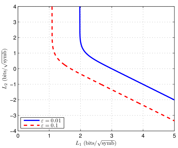
Figure 6.3: Illustration of $\mathcal{L}(\varepsilon;R_{1}^{*},R_{2}^{*})$ in (6.17) for the source $P_{X_{1}X_{2}}$ in (6.18) with $\varepsilon=0.01,0.1$. The regions are to the top right of the boundaries indicated.

The region $\mathcal{L}(\varepsilon;R_{1}^{*},R_{2}^{*})$ for Case (iii) is illustrated in Fig. 6.3 for a binary source $(X_{1},X_{2})$ with distribution

$$P_{X_{1}X_{2}}(x_{1},x_{2})=\begin{bmatrix}0.7&0.1\\ 0.1&0.1\end{bmatrix}.$$ (6.18)

Note that $\mathcal{L}(\varepsilon;R_{1}^{*},R_{2}^{*})$ for other points on the boundary can be found by symmetry. For example for the horizontal boundary, simply interchange the indices $1$ and $2$ in (6.15). The case in which $\mathbf{V}$ is not positive definite was dealt with in detail in [157].

6.2.3 Proof of Main Result and Remarks

Proof.

The proof of the direct part specializes the non-asymptotic bound in Proposition 6.1 with the choice $\gamma=n^{1/4}$. Choose code sizes $M_{1n}$ and $M_{2n}$ to be the smallest integers satisfying

$$\log M_{jn} \geq nR_{j}^{*}+\sqrt{n}L_{j}+2n^{1/4},\quad j=1,2,$$ (6.19)

for some $(L_{1},L_{2})\in\mathbb{R}^{2}$. Substitute these choices into the probability in (6.4), denoted as $\mathfrak{p}$. The complementary probability $1-\mathfrak{p}$ is

$$1\!-\!\mathfrak{p}\!=\!\Pr\left(\mathbf{h}_{X_{1}^{n}X_{2}^{n}}(X_{1}^{n},X_{2}^{n})\!<\!\begin{bmatrix}nR_{1}^{*}+\sqrt{n}L_{1}+n^{1/4}\\ nR_{2}^{*}+\sqrt{n}L_{2}+n^{1/4}\\ n(R_{1}^{*}\!+\!R_{2}^{*})\!+\!\sqrt{n}(L_{1}\!+\!L_{2})\!+\!3n^{1/4}\end{bmatrix}\right).$$ (6.20)

Recall that $\mathbf{h}_{X_{1}^{n}X_{2}^{n}}(\mathbf{x}_{1},\mathbf{x}_{2})$ is the entropy density in (6.6) and that inequalities (like $<$) are applied element-wise. The three events in the probability above are

$$\mathcal{A}_{1} \!:=\!\bigg{\{}\frac{1}{n}\log\frac{1}{P_{X_{1}^{n}|X_{2}^{n}}(X_{1}^{n}|X_{2}^{n})}\!<\!R_{1}^{*}\!+\!\frac{L_{1}}{\sqrt{n}}+n^{-3/4}\bigg{\}},$$ (6.21)

$$\mathcal{A}_{2} \!:=\!\bigg{\{}\frac{1}{n}\log\frac{1}{P_{X_{2}^{n}|X_{1}^{n}}(X_{2}^{n}|X_{1}^{n})}\!<\!R_{2}^{*}\!+\!\frac{L_{2}}{\sqrt{n}}+n^{-3/4}\bigg{\}},\quad\mbox{and}$$ (6.22)

$$\mathcal{A}_{12} \!:=\!\bigg{\{}\frac{1}{n}\log\frac{1}{P_{X_{1}^{n}X_{2}^{n}}(X_{1}^{n},X_{2}^{n})}\!<\!R_{1}^{*}\!+\!R_{2}^{*}\!+\!\frac{L_{1}\!+\!L_{2}}{\sqrt{n}}+3n^{-3/4}\bigg{\}}.$$ (6.23)

As such, the probability in (6.20) is $\Pr(\mathcal{A}_{1}\cap\mathcal{A}_{2}\cap\mathcal{A}_{12})$.

Let us consider Case (i) in Theorem 6.1. In this case, $R_{2}^{*}>H(X_{2})$ and $R_{1}^{*}+R_{2}^{*}>H(X_{1},X_{2})$. By the weak law of large numbers, $\Pr(\mathcal{A}_{2})\to 1$ and $\Pr(\mathcal{A}_{12})\to 1$ as $n$ grows. In fact, these probabilities converge to one exponentially fast. Thus,

$$1-\mathfrak{p}\geq\Pr(\mathcal{A}_{1})+\exp(-n\xi)$$ (6.24)

for some $\xi>0$. Furthermore, because $R_{1}^{*}=H(X_{1}|X_{2})$, $\Pr(\mathcal{A}_{1})$ can be estimated using the Berry-Esseen theorem as

$$\Pr(\mathcal{A}_{1})\geq\Phi\bigg{(}\frac{L_{1}}{\sqrt{V(X_{1}|X_{2})}}\bigg{)}+O(n^{-1/4}).$$ (6.25)

Hence, one has

$$\mathfrak{p}\leq 1-\Phi\bigg{(}\frac{L_{1}}{\sqrt{V(X_{1}|X_{2})}}\bigg{)}+O(n^{-1/4}).$$ (6.26)

Coupled with the fact that $\exp(-\gamma)=\exp(-n^{1/4})$, the proof of the direct part of (6.15) is complete. The converse employs essentially the same technique. Case (ii) is also similar with the exception that now $\Pr(\mathcal{A}_{1})\to 1$ and $\Pr(\mathcal{A}_{2})\to 1$, while $\Pr(\mathcal{A}_{12})$ is estimated using the Berry-Esseen theorem.

We are left with Case (iii). In this case, only $\Pr(\mathcal{A}_{2})\to 1$. Thus, just as in (6.24), (6.20) can be estimated as

$$1-\mathfrak{p}\geq\Pr(\mathcal{A}_{1}\cap\mathcal{A}_{12})+\exp(-n\xi^{\prime})$$ (6.27)

for some $\xi^{\prime}>0$. The probability can now be estimated using the multivariate Berry-Esseen theorem (Corollary 1.1) as

$$\Pr(\mathcal{A}_{1}\cap\mathcal{A}_{12})\geq\Psi\big{(}L_{1},L_{1}+L_{2};\mathbf{0},\mathbf{V}_{1,12}\big{)}+O(n^{-1/4}).$$ (6.28)

We complete the proof of (6.17) similarly to Case (i). The converse is completely analogous. ∎

A couple of take-home messages are in order:

First, consider Case (i). In this case, we are operating “far away” from the constraint concerning the second rate and the sum rate constraint. This corresponds to the events $\mathcal{A}_{2}^{c}$ and $\mathcal{A}_{12}^{c}$. Thus, by the theory of large deviations, $\Pr(\mathcal{A}_{2}^{c})$ and $\Pr(\mathcal{A}_{12}^{c})$ both tend to zero exponentially fast. Essentially for these two error events, we are in the error exponents regime. The same holds true for Case (ii).

Second, consider Case (iii). This is the most interesting case for the second-order asymptotics for the Slepian-Wolf problem. We are operating at a corner point and are far away from the second rate constraint, i.e., in the error exponents regime for $\mathcal{A}_{2}^{c}$. The remaining two events $\mathcal{A}_{1}$ and $\mathcal{A}_{12}$ are, however, still in the central limit regime and hence their joint probability must be estimated using the multivariate Berry-Esseen theorem. Instead of the result being expressible in terms of a univariate Gaussian cdf $\Phi$ (which is the case for single-terminal problems in Part II of this monograph), the multivariate version of the Gaussian cdf $\Psi$, parameterized by the (in general, full) covariance matrix $\mathbf{V}_{1,12}$ in (6.14), must be employed. Compared to the cooperative case where $X_{2}^{n}$ (resp. $X_{1}^{n}$) is available to encoder $1$ (resp. encoder $2$), we see from the result in Case (iii) that Slepian-Wolf coding, in general, incurs a rate-loss over the case where side-information is available to all terminals. Indeed, when side-information is available at all terminals, the matrix $\mathbf{V}_{1,12}$ that characterizes $\mathcal{L}(\varepsilon;R_{1}^{*},R_{2}^{*})$ in Case (iii) would be diagonal [157], since the source coding problems involving $X_{1}$ and $X_{2}$ are now independent of each other. In other words, in this case, there exists a sequence of codes with error probabilities $\varepsilon_{n}$ satisfying (6.8) and sizes $(M_{1n},M_{2n})$ satisfying

$$\log M_{1n} \leq nH(X_{1}|X_{2})-\sqrt{nV(X_{1}|X_{2})}\Phi^{-1}(\varepsilon)+o(\sqrt{n}),$$ (6.29)

$$\log M_{2n} \leq nH(X_{2}|X_{1})-\sqrt{nV(X_{2}|X_{1})}\Phi^{-1}(\varepsilon)+o(\sqrt{n}),$$ (6.30)

$$\log(M_{1n}M_{2n}) \leq nH(X_{1},X_{2})-\sqrt{nV(X_{1},X_{2})}\Phi^{-1}(\varepsilon)+o(\sqrt{n}).$$ (6.31)

Inequality (6.29) corresponds to the problem of source coding $X_{1}$ with $X_{2}$ available as full (non-coded) side information at the decoder. Inequality (6.30) swaps the role of $X_{1}$ and $X_{2}$. Finally, inequality (6.31) corresponds to lossless source coding of the vector source $(X_{1},X_{2})$, similarly to the result on lossless source coding without side information in Section 3.2.

6.3 Second-Order Asymptotics of Slepian-Wolf Coding via the Method of Types

Just as in Section 3.3 (second-order asymptotics of lossless data compression via the method of types), we can show that codes that do not necessarily have to have full knowledge of the source statistics (i.e., partially universal source codes) can achieve the second-order coding rate region $\mathcal{L}(\varepsilon;R_{1}^{*},R_{2}^{*})$. However, the coding scheme does require the knowledge of the entropies together with the pair of second-order rates $(L_{1},L_{2})$ we would like to achieve. We illustrate the achievability proof technique for Case (iii) of Theorem 6.1, in which $R_{1}^{*}=H(X_{1}|X_{2})$ and $R_{2}^{*}=H(X_{2})$.

The code construction is based on Cover’s random binning idea [32] and the decoding strategy is similar to minimum empirical entropy decoding [38, 39]. Fix $(L_{1},L_{2})\in\mathcal{L}(\varepsilon;R_{1}^{*},R_{2}^{*})$ where $\mathcal{L}(\varepsilon;R_{1}^{*},R_{2}^{*})$ is given in (6.17). Also fix code sizes $M_{1n}$ and $M_{2n}$ satisfying (6.19). For each $j=1,2$, uniformly and independently assign each sequence $\mathbf{x}_{j}\in\mathcal{X}_{j}^{n}$ into one of $M_{jn}$ bins labeled as $\mathcal{B}_{j}(m_{j}),m_{j}\in\{1,\ldots,M_{jn}\}$. The bin assignments are revealed to all parties. To send $\mathbf{x}_{j}\in\mathcal{X}_{j}^{n}$, encoder $j$ transmits its bin index $m_{j}$.

The decoder, upon receipt of the bin indices $(m_{1},m_{2})\in\{1,\ldots,M_{1n}\}\times\{1,\ldots,M_{2n}\}$, finds a pair of sequences $(\hat{\mathbf{x}}_{1},\hat{\mathbf{x}}_{2})\in\mathcal{B}_{1}(m_{1})\times\mathcal{B}_{2}(m_{2})$ satisfying

$$\hat{\mathbf{H}}(\mathbf{x}_{1},\mathbf{x}_{2}):=\begin{bmatrix}\hat{H}(\mathbf{x}_{1}|\mathbf{x}_{2})\\ \hat{H}(\mathbf{x}_{2}|\mathbf{x}_{1})\\ \hat{H}(\mathbf{x}_{1},\mathbf{x}_{2})\end{bmatrix}\leq\begin{bmatrix}\gamma_{1}\\ \gamma_{2}\\ \gamma_{12}\end{bmatrix}=:\bm{\gamma}$$ (6.32)

for some thresholds $\gamma_{1},\gamma_{2},\gamma_{12}$ defined as

$$\gamma_{1} :=H(X_{1}|X_{2})+\frac{L_{1}}{\sqrt{n}}+n^{-1/4}$$ (6.33)

$$\gamma_{2} :=H(X_{2})+\frac{L_{2}}{\sqrt{n}}+n^{-1/4}$$ (6.34)

$$\gamma_{12} :=H(X_{1},X_{2})+\frac{L_{1}+L_{2}}{\sqrt{n}}+n^{-1/4}$$ (6.35)

If there is no sequence pair $(\hat{\mathbf{x}}_{1},\hat{\mathbf{x}}_{2})\in\mathcal{B}_{1}(m_{1})\times\mathcal{B}_{2}(m_{2})$ satisfying (6.32) or if there is more than one, declare an error. Note that the thresholds depend on the entropies and $(L_{1},L_{2})$, hence these values need to be known to the decoder.

Let the generated source sequences be $X_{1}^{n}$ and $X_{2}^{n}$ and their associated bin indices be $M_{1}=M_{1}(X_{1}^{n})$ and $M_{2}=M_{2}(X_{2}^{n})$ respectively. By symmetry, we may assume that $M_{1}=M_{2}=1$. The error events are as follows:

$$\mathcal{E}_{0} :=\big{\{}\hat{\mathbf{H}}(X_{1}^{n},X_{2}^{n})\not\leq\bm{\gamma}\big{\}},$$ (6.36)

$$\mathcal{E}_{1} :=\big{\{}\exists\,\tilde{\mathbf{x}}_{1}\in\mathcal{B}_{1}(1):\tilde{\mathbf{x}}_{1}\neq X_{1}^{n},\hat{\mathbf{H}}(\tilde{\mathbf{x}}_{1},X_{2}^{n})\leq\bm{\gamma}\big{\}},$$ (6.37)

$$\mathcal{E}_{2} :=\big{\{}\exists\,\tilde{\mathbf{x}}_{2}\in\mathcal{B}_{2}(1):\tilde{\mathbf{x}}_{2}\neq X_{2}^{n},\hat{\mathbf{H}}(X_{1}^{n},\tilde{\mathbf{x}}_{2})\leq\bm{\gamma}\big{\}},\quad\mbox{and}$$ (6.38)

$$\mathcal{E}_{12} :=\big{\{}\exists\,(\tilde{\mathbf{x}}_{1},\tilde{\mathbf{x}}_{2})\in\mathcal{B}_{1}(1)\times\mathcal{B}_{2}(1):\tilde{\mathbf{x}}_{1}\neq X_{1}^{n},\tilde{\mathbf{x}}_{2}\neq X_{2}^{n},$$

$$\qquad\qquad\hat{\mathbf{H}}(\tilde{\mathbf{x}}_{1},\tilde{\mathbf{x}}_{2})\leq\bm{\gamma}\big{\}}.$$ (6.39)

Let $\mathbf{H}(X_{1},X_{2})=[H(X_{1}|X_{2}),H(X_{2}|X_{1}),H(X_{1},X_{2})]^{\prime}$. It can be verified that the following central limit relation holds [157]:

$$\sqrt{n}\big{(}\hat{\mathbf{H}}(X_{1}^{n},X_{2}^{n})-\mathbf{H}(X_{1},X_{2})\big{)}\stackrel{{\scriptstyle\mathrm{d}}}{{\longrightarrow}}\mathcal{N}\big{(}\mathbf{0},\mathbf{V}\big{)}.$$ (6.40)

This is the multi-dimensional analogue of (3.35) for almost lossless source coding. Thus, by the same argument as that in (6.27)–(6.28) (ignoring the second entry in $\hat{\mathbf{H}}(X_{1}^{n},X_{2}^{n})$ because $R_{2}^{*}=H(X_{2})>H(X_{2}|X_{1})$), one has

$$\Pr(\mathcal{E}_{0})\leq\varepsilon+O(n^{-1/4}).$$ (6.41)

Furthermore, by using the method of types, we may verify that

$$\Pr(\mathcal{E}_{1}) \!\leq\!\sum_{\mathbf{x}_{1},\mathbf{x}_{2}}P_{X_{1}^{n}X_{2}^{n}}(\mathbf{x}_{1},\mathbf{x}_{2})\sum_{\tilde{\mathbf{x}}_{1}\neq\mathbf{x}_{1}:\hat{\mathbf{H}}(\tilde{\mathbf{x}}_{1},\mathbf{x}_{2})\leq\bm{\gamma}}\Pr\big{(}\tilde{\mathbf{x}}_{1}\in\mathcal{B}_{1}(1)\big{)}$$ (6.42)

$$\!\leq\!\sum_{\mathbf{x}_{1},\mathbf{x}_{2}}P_{X_{1}^{n}X_{2}^{n}}(\mathbf{x}_{1},\mathbf{x}_{2})\sum_{\tilde{\mathbf{x}}_{1}\neq\mathbf{x}_{1}:\hat{H}(\tilde{\mathbf{x}}_{1}|\mathbf{x}_{2})\leq\gamma_{1}}\Pr\big{(}\tilde{\mathbf{x}}_{1}\in\mathcal{B}_{1}(1)\big{)}$$ (6.43)

$$\!=\!\sum_{\mathbf{x}_{1},\mathbf{x}_{2}}P_{X_{1}^{n}X_{2}^{n}}(\mathbf{x}_{1},\mathbf{x}_{2})\sum_{\tilde{\mathbf{x}}_{1}\neq\mathbf{x}_{1}:\hat{H}(\tilde{\mathbf{x}}_{1}|\mathbf{x}_{2})\leq\gamma_{1}}\frac{1}{M_{1n}}$$ (6.44)

$$\!\leq\!\sum_{\mathbf{x}_{1},\mathbf{x}_{2}}P_{X_{1}^{n}X_{2}^{n}}(\mathbf{x}_{1},\mathbf{x}_{2})\sum_{\begin{subarray}{c}V\in\mathscr{V}_{n}(\mathcal{X}_{2};P_{\mathbf{x}_{2}}):\\ H(V|P_{\mathbf{x}_{2}})\leq\gamma_{1}\end{subarray}}\sum_{\tilde{\mathbf{x}}_{1}\in\mathcal{T}_{V}(\mathbf{x}_{2})}\frac{1}{M_{1n}}$$ (6.45)

$$\!\leq\!\sum_{\mathbf{x}_{1},\mathbf{x}_{2}}P_{X_{1}^{n}X_{2}^{n}}(\mathbf{x}_{1},\mathbf{x}_{2})\sum_{\begin{subarray}{c}V\in\mathscr{V}_{n}(\mathcal{X}_{2};P_{\mathbf{x}_{2}}):\\ H(V|P_{\mathbf{x}_{2}})\leq\gamma_{1}\end{subarray}}\frac{\exp\big{(}nH(V|P_{\mathbf{x}_{2}})\big{)}}{M_{1n}}$$ (6.46)

$$\!\leq\!\sum_{\mathbf{x}_{1},\mathbf{x}_{2}}P_{X_{1}^{n}X_{2}^{n}}(\mathbf{x}_{1},\mathbf{x}_{2})\sum_{\begin{subarray}{c}V\in\mathscr{V}_{n}(\mathcal{X}_{2};P_{\mathbf{x}_{2}}):\\ H(V|P_{\mathbf{x}_{2}})\leq\gamma_{1}\end{subarray}}\frac{\exp\big{(}n\gamma_{1}\big{)}}{M_{1n}}$$ (6.47)

$$\!\leq\!(n+1)^{|\mathcal{X}_{1}||\mathcal{X}_{2}|}\exp(-n^{1/4}),$$ (6.48)

where in (6.44) we used the uniformity of the binning, in (6.45) we partitioned the set of sequences $\tilde{\mathbf{x}}_{1}$ into conditional types given $\mathbf{x}_{2}$ and in (6.46), we used the fact that $|\mathcal{T}_{V}(\mathbf{x}_{2})|\leq\exp\big{(}nH(V|P_{\mathbf{x}_{2}})\big{)}$ (cf. Lemma 1.2). Finally, the type counting lemma and the choices of $\gamma_{1}$ and $M_{1n}$ were used in (6.48). The same calculation can be performed for $\Pr(\mathcal{E}_{2})$ and $\Pr(\mathcal{E}_{12})$. Thus, asymptotically, the error probability is no larger than $\varepsilon$, as desired.

6.4 Other Fixed Error Asymptotic Notions

In the preceding sections, we were solely concerned with the deviations of order $\Theta(\frac{1}{\sqrt{n}})$ away from the first-order fundamental limit $(R_{1}^{*},R_{2}^{*})$. However, one may also be interested in other metrics that quantify backoffs from particular first-order fundamental limits. Here we mention three other quantities that have appeared in the literature.

6.4.1 Weighted Sum-Rate Dispersion

For constants $\alpha,\beta\geq 0$, the minimum value of $\alpha R_{1}+\beta R_{2}$ for asymptotically achievable $(R_{1},R_{2})$ is called the optimal weighted sum-rate. Of particular interest is the case $\alpha=\beta=1$, corresponding to the standard sum-rate $R_{1}+R_{2}$, but other cases may be important as well, e.g., if transmitting from encoder $1$ is more costly than transmitting from encoder $2$. Because of the polygonal shape of the optimal region described in the Slepian-Wolf region in (6.1), the optimal weighted sum-rate is always achieved at (at least) one of the two corner points, and the optimal rate is given by

$$R_{\mathrm{sum}}^{*}(\alpha,\beta):=\left\{\begin{array}[]{cc}\alpha H(X_{1}|X_{2})+\beta H(X_{2})&\alpha\geq\beta\\ \alpha H(X_{1})+\beta H(X_{2}|X_{1})&\alpha<\beta\end{array}\right..$$ (6.49)

One can then define $J\in\mathbb{R}$ to be an achievable $(\varepsilon,\alpha,\beta)$-weighted second-order coding rate if there exists a sequence of $(M_{1n},M_{2n},\varepsilon_{n})$-codes for the correlated source $P_{X_{1}^{n}X_{2}^{n}}$ such that the error probability condition in (6.8) holds and

$$\limsup_{n\to\infty}\frac{1}{\sqrt{n}}\big{(}\alpha\log M_{1n}+\beta\log M_{2n}-nR_{\mathrm{sum}}^{*}(\alpha,\beta)\big{)}\leq J.$$ (6.50)

In [157], the smallest such $J$, denoted as $J^{*}(\varepsilon;\alpha,\beta)$, was found using a proof technique similar to that for Theorem 6.1.

6.4.2 Dispersion-Angle Pairs

One can also imagine approaching a point on the boundary $(R_{1}^{*},R_{2}^{*})$ fixing an angle of approach $\theta\in[0,2\pi)$. Let $(F,\theta)$ be called an achievable $(\varepsilon,R_{1}^{*},R_{2}^{*})$-dispersion-angle pair if there exists a sequence of $(M_{1n},M_{2n},\varepsilon_{n})$-codes for the correlated source $P_{X_{1}^{n}X_{2}^{n}}$ such that the error probability condition in (6.8) holds and

$$\limsup_{n\to\infty}\frac{1}{\sqrt{n}}\big{(}\log M_{1n}-nR_{1}^{*}\big{)} \leq\sqrt{F}\,\cos\theta,\quad\mbox{and}$$ (6.51)

$$\limsup_{n\to\infty}\frac{1}{\sqrt{n}}\big{(}\log M_{2n}-nR_{2}^{*}\big{)} \leq\sqrt{F}\,\sin\theta.$$ (6.52)

Clearly, dispersion-angle pairs $(F,\theta)$ are in one-to-one correspondence with second-order coding rate pairs $(L_{1},L_{2})$. The minimum such $F$ for a given $\theta$, denoted as $F^{*}(\theta,\varepsilon;R_{1}^{*},R_{2}^{*})$, measures the speed of approach to $(R_{1}^{*},R_{2}^{*})$ at an angle $\theta$. This fundamental quantity $F^{*}(\theta,\varepsilon;R_{1}^{*},R_{2}^{*})$ was also characterized in [157].

6.4.3 Global Approaches

Authors of early works on second-order asymptotics in multi-terminal systems [84, 111, 156] considered global rate regions, meaning that they were concerned with quantifying the sizes $(M_{1n},M_{2n})$ of length-$n$ block codes with error probability not exceeding $\varepsilon$. These sizes are called $(n,\varepsilon)$-achievable. In the Slepian-Wolf context, a result by Tan-Kosut [156] states that $(M_{1n},M_{2n})$ are $(n,\varepsilon)$-achievable iff

$$\begin{bmatrix}\log M_{1n}\\ \log M_{2n}\\ \log(M_{1n}M_{2n})\end{bmatrix}\!\in\!\begin{bmatrix}nH(X_{1}|X_{2})\\ nH(X_{2}|X_{1})\\ nH(X_{1},X_{2})\end{bmatrix}\!-\!\sqrt{n}\Psi^{-1}(\mathbf{V},\varepsilon)\!+\!O\left(\log n\right)\mathbf{1}$$ (6.53)

where ${\Psi^{-1}}(\mathbf{V},\varepsilon)$ is an appropriate generalization of the $\Phi^{-1}$ function and $\mathbf{1}$ is the vector of all ones. The precise definition of $\Psi^{-1}(\mathbf{V},\varepsilon)$, given in (8.24) and illustrated Fig. 8.3, will not be of concern here.

While statements such as (6.53) are mathematically correct and are reminiscent of asymptotic expansions in the point-to-point case (cf. that for lossless source coding in (3.14)), they do not provide the complete picture with regard to the convergence of rate pairs to a fundamental limit, e.g., a corner point of the Slepian-Wolf region. Indeed, an achievability statement similar to (6.53) holds for the DM-MAC for each input distribution [84, 111, 136, 156] and hence the union over all input distributions. However, one of the major deficiencies of such a statement is that the $O(\log n)$ third-order term is not uniform in the input distributions; this poses serious challenges in the interpretation of the result if we consider random coding using a sequence of input distributions that varies with the blocklength (cf. Chapter 8). Thus, as pointed out by Haim-Erez-Kochman [65], for multi-user problems, the value of global expansions such as that in (6.53) is limited, and can only be regarded as stepping stones to obtain local results (if possible). Indeed, we do this for the Gaussian MAC with degraded message sets in Chapter 8.

The main takeaway of this section is that one should adopt the local, weighted sum-rate, or dispersion-angle problem setups to analyze the second-order asymptotics for multi-terminal problems. These setups are information-theoretic in nature. In particular, operational quantities (such as the set $\mathcal{L}(\varepsilon;R_{1}^{*},R_{2}^{*})$ or the number $F^{*}(\theta,\varepsilon;R_{1}^{*},R_{2}^{*})$) are defined then equated to information quantities.

Chapter 7 A Special Class of Gaussian Interference Channels

This chapter presents results on second-order asymptotics for a channel-type network information theory problem. The problem we consider here is a special case of the two-sender, two-receiver interference channel (IC) shown in Fig. 7.1. This model is a basic building block in many modern wireless systems, so theoretical results and insights are of tremendous practical relevance. The IC was first studied by Ahlswede [2] who established basic bounds on the capacity region. However, the capacity region for the discrete memoryless and Gaussian memoryless cases have remained as open problems for over $40$ years except for some very special cases. The best known inner bound is due to Han and Kobayashi [70]. A simplified form of the Han-Kobayashi inner bound was presented by Chong-Motani-Garg-El Gamal [26].

Figure 7.1: Illustration of the interference channel problem.

Since the determination of the capacity region is formidable, the derivation of conclusive results for the second-order asymptotics of general memoryless ICs is also beyond us at this point in time. One very special case in which the capacity region is known is the IC with very strong interference (VSI). In this case, the intuition is that each receiver can reliably decode the non-intended message which then aids in decoding the intended message. The capacity region for the discrete memoryless IC with VSI consists of the set of rate pairs $(R_{1},R_{2})$ satisfying

$$R_{1}\leq I(X_{1};Y_{1}|X_{2},Q),\quad\mbox{and}\quad R_{2}\leq I(X_{2};Y_{2}|X_{1},Q)$$ (7.1)

for some $P_{Q},P_{X_{1}|Q}$ and $P_{X_{2}|Q}$, where $Q$ is known as the time-sharing random variable. In the Gaussian case in which Carleial [22] studied, the above region can be written more explicitly as

$$R_{1}\leq\mathsf{C}(\mathsf{snr}_{1})\quad\mbox{and}\quad R_{2}\leq\mathsf{C}(\mathsf{snr}_{2}),$$ (7.2)

where $\mathsf{snr}_{j}$ is the signal-to-noise ratio of the direct channel from sender $j$ to receiver $j$ and the Gaussian capacity function is defined as $\mathsf{C}(\mathsf{snr}):=\frac{1}{2}\log(1+\mathsf{snr})$. See Fig. 7.2 for an illustration of the capacity region and the monograph by Shang and Chen [140] for further discussions on Gaussian interference channels. Carleial’s result is surprising because it appears that interference does not reduce the capacity of the constituent channels since $\mathsf{C}(\mathsf{snr}_{j})$ is the capacity of the $j^{\mathrm{th}}$ channel. In Carleial’s own words [22],

“Very strong interference is as innocuous as no interference at all.”

Similarly to the discrete case in (7.1), the (first-order optimal) achievability proof strategy for the Gaussian case involves first decoding the interference, subtracting it off from the received channel output, and finally, reliably decoding the intended message. The VSI condition ensures that the rate constraints in (7.2), representing requirement for the second decoding steps to succeed, dominate.

In this chapter, we make a slightly stronger assumption compared to that made by Carleial [22]. We assume that the inequalities that define the VSI condition are strict; we call this the strictly VSI (SVSI) assumption/regime. With this assumption, we are able to derive the second-order asymptotics of this class of Gaussian ICs.

Although the main result in this chapter appears to be similar to the Slepian-Wolf case (in Chapter 6), there are several take-home messages that differ from the simpler Slepian-Wolf problem.

1. First, similar to Carleial’s observation that for Gaussian ICs with VSI the capacity is not reduced, we show that the dispersions are not affected under the SVSI assumption. More precisely, the second-order coding rate region (a set similar to that for the Slepian-Wolf problem in Chapter 6), is characterized entirely in terms of the dispersions $\mathsf{V}(\mathsf{snr}_{j})$ of the two direct AWGN channels from encoder $j$ to decoder $j$;

2. Second, the main result in this chapter suggests that under the SVSI assumption, and in the second-order asymptotic setting, the two error events (of incorrectly decoding messages $1$ and $2$) are almost independent;

3. Third, for the direct part, we demonstrate the utility of an achievability proof technique by MolavianJazi-Laneman [112] that is also applicable to our problem of Gaussian ICs with SVSI. This technique is, in general, applicable to multi-terminal Gaussian channels. In the asymptotic evaluation of the information spectrum bound (Feinstein bound [53]), the problem is “lifted” to higher dimensions to facilitate the application of limit theorems for independent random vectors;

This chapter is based on work by Le, Tan and Motani [103].

7.1 Definitions and Non-Asymptotic Bounds

Let us now state the Gaussian IC problem. The Gaussian IC is defined by the following input-output relation:

$$Y_{1i} =g_{11}X_{1i}+g_{12}X_{2i}+Z_{1i},$$ (7.3)

$$Y_{2i} =g_{21}X_{1i}+g_{22}X_{2i}+Z_{2i},$$ (7.4)

where $i=1,\ldots,n$ and $g_{jk}$ are the channel gains from sender $k$ to receiver $j$ and $Z_{1i}\sim\mathcal{N}(0,1)$ and $Z_{2i}\sim\mathcal{N}(0,1)$ are independent noise components. Thus, the channel from $(x_{1},x_{2})$ to $(y_{1},y_{2})$ is

$$W(y_{1},y_{2}|x_{1},x_{2})=\frac{1}{2\pi}\exp\Bigg{(}-\frac{1}{2}\bigg{\|}\begin{bmatrix}y_{1}\\ y_{2}\end{bmatrix}-\begin{bmatrix}g_{11}&g_{12}\\ g_{21}&g_{22}\end{bmatrix}\begin{bmatrix}x_{1}\\ x_{2}\end{bmatrix}\bigg{\|}_{2}^{2}\Bigg{)}.$$ (7.5)

Let $W_{1}$ and $W_{2}$ denote the marginals of $W$. The channel also acts in a stationary, memoryless way so

$$W^{n}(\mathbf{y}_{1},\mathbf{y}_{2}|\mathbf{x}_{1},\mathbf{x}_{2})=\prod_{i=1}^{n}W(y_{1i},y_{2i}|x_{1i},x_{2i}).$$ (7.6)

It will be convenient to make the dependence of the code on the blocklength explicit right away. We define an $(n,M_{1},M_{2},S_{1},S_{2},\varepsilon)$-code for the Gaussian IC as four maps that consists of two encoders $f_{j}:\{1,\ldots,M_{j}\}\to\mathbb{R}^{n},j=1,2$ and two decoders $\varphi_{j}:\mathbb{R}^{n}\to\{1,\ldots,M_{j}\}$ such that the following power constraints are satisfied

$$\big{\|}f_{j}(m_{j})\big{\|}_{2}^{2}=\sum_{i=1}^{n}f_{ji}(m_{j})^{2}\leq nS_{j}$$ (7.7)

and, denoting $\mathcal{D}_{m_{1},m_{2}}:=\{(\mathbf{y}_{1},\mathbf{y}_{2}):\varphi_{1}(\mathbf{y}_{1})=m_{1}\mbox{ and }\varphi_{2}(\mathbf{y}_{2})=m_{2}\}$ as the decoding region for $(m_{1},m_{2})$, the average error probability

$$\frac{1}{M_{1}M_{2}}\sum_{m_{1}=1}^{M_{1}}\sum_{m_{2}=1}^{M_{2}}W^{n}\big{(}\mathbb{R}^{n}\times\mathbb{R}^{n}\setminus\mathcal{D}_{m_{1},m_{2}}\big{|}f_{1}(m_{1}),f_{2}(m_{2})\big{)}\leq\varepsilon.$$ (7.8)

In (7.7), $S_{1}$ and $S_{2}$ are the admissible powers on the codewords $f_{1}(m_{1})$ and $f_{2}(m_{2})$. The signal-to-noise ratios of the direct channels are

$$\mathsf{snr}_{1}:=g_{11}^{2}S_{1},\quad\mbox{and}\quad\mathsf{snr}_{2}:=g_{22}^{2}S_{2}.$$ (7.9)

The interference-to-noise ratios are

$$\mathsf{inr}_{1}:=g_{12}^{2}S_{2},\quad\mbox{and}\quad\mathsf{inr}_{2}:=g_{21}^{2}S_{1}.$$ (7.10)

We say that the Gaussian IC $W$, together with the transmit powers $(S_{1},S_{2})$, is in the VSI regime if the signal- and interference-to-noise ratios satisfy

$$\mathsf{snr}_{1}\leq\frac{\mathsf{inr}_{2}}{1+\mathsf{snr}_{2}},\quad\mbox{and}\quad\mathsf{snr}_{2}\leq\frac{\mathsf{inr}_{1}}{1+\mathsf{snr}_{1}},$$ (7.11)

or equivalently, in terms of capacities,

$$\mathsf{C}(\mathsf{snr}_{1})+\mathsf{C}(\mathsf{snr}_{2})\leq\min\{\mathsf{C}(\mathsf{snr}_{1}+\mathsf{inr}_{1}),\mathsf{C}(\mathsf{snr}_{2}+\mathsf{inr}_{2})\}.$$ (7.12)

The Gaussian IC is in the SVSI regime if the inequalities in (7.11)–(7.12) are strict. Intuitively, the VSI (or SVSI) assumption means that the cross channel gains $g_{12}$ and $g_{21}$ are much stronger (larger) than the direct gains $g_{11}$ and $g_{22}$ for given transmit powers $S_{1}$ and $S_{2}$.

We now state non-asymptotic bounds that are evaluated asymptotically later. The proofs of these bounds are standard. See [66] or [103].

Proposition 7.1 (Achievability bound for IC).

Fix any input distributions $P_{X_{1}^{n}}$ and $P_{X_{2}^{n}}$ whose support satisfies the power constraints in (7.7), i.e., $\|X_{j}^{n}\|_{2}\leq nS_{j}$ with probability one. For every $n\in\mathbb{N}$, every $\gamma>0$ and for any choice of (conditional) output distributions $Q_{Y_{1}^{n}|X_{2}^{n}}$, $Q_{Y_{2}^{n}|X_{1}^{n}}$, $Q_{Y_{1}^{n}}$ and $Q_{Y_{2}}^{n}$ there exists an $(n,M_{1},M_{2},S_{1},S_{2},\varepsilon)$-code for the IC such that

$$\varepsilon\leq\Pr\bigg{(}\log\frac{W_{1}^{n}(Y_{1}^{n}|X_{1}^{n},X_{2}^{n})}{Q_{Y_{1}^{n}|X_{2}^{n}}(Y_{1}^{n}|X_{2}^{n})} \leq\log M_{1}+n\gamma\quad\mbox{or }$$

$$\log\frac{W_{2}^{n}(Y_{2}^{n}|X_{1}^{n},X_{2}^{n})}{Q_{Y_{2}^{n}|X_{1}^{n}}(Y_{2}^{n}|X_{1}^{n})} \leq\log M_{2}+n\gamma\quad\mbox{or }$$

$$\log\frac{W_{1}^{n}(Y_{1}^{n}|X_{1}^{n},X_{2}^{n})}{Q_{Y_{1}^{n}}(Y_{1}^{n})} \leq\log(M_{1}M_{2})\!+\!n\gamma\quad\mbox{or }$$

$$\log\frac{W_{2}^{n}(Y_{2}^{n}|X_{1}^{n},X_{2}^{n})}{Q_{Y_{2}^{n}}(Y_{2}^{n})} \leq\log(M_{1}M_{2})\!+\!n\gamma\bigg{)}+\zeta\exp(-n\gamma),$$ (7.13)

where $\zeta:=\sum_{k=1}^{2}\sum_{j=1}^{2}\zeta_{jk}$ and

$$\zeta_{11} :=\sup_{\mathbf{x}_{2},\mathbf{y}_{1}}\frac{P_{X_{1}^{n}}W_{1}^{n}(\mathbf{y}_{1}|\mathbf{x}_{2})}{Q_{Y_{1}^{n}|X_{2}^{n}}(\mathbf{y}_{1}|\mathbf{x}_{2})},\quad\zeta_{12}:=\sup_{\mathbf{y}_{1}}\frac{P_{X_{1}^{n}}P_{X_{2}^{n}}W_{1}^{n}(\mathbf{y}_{1})}{Q_{Y_{1}^{n}}(\mathbf{y}_{1})}$$ (7.14)

$$\zeta_{21} :=\sup_{\mathbf{x}_{1},\mathbf{y}_{2}}\frac{P_{X_{2}^{n}}W_{2}^{n}(\mathbf{y}_{2}|\mathbf{x}_{1})}{Q_{Y_{2}^{n}|X_{1}^{n}}(\mathbf{y}_{2}|\mathbf{x}_{1})},\quad\zeta_{22}:=\sup_{\mathbf{y}_{2}}\frac{P_{X_{1}^{n}}P_{X_{2}^{n}}W_{2}^{n}(\mathbf{y}_{2})}{Q_{Y_{2}^{n}}(\mathbf{y}_{2})}$$ (7.15)

This is a generalization of the average error version of Feinstein’s lemma [53] (Proposition 4.1). Notice that we have the freedom to choose the output distributions at the cost of having to control the ratios $\zeta_{jk}$ of the induced output distributions and our choice of output distributions.

Proposition 7.2 (Converse bound for IC).

For every $n\in\mathbb{N}$, every $\gamma>0$ and for any choice of (conditional) output distributions $Q_{Y_{1}^{n}|X_{2}^{n}}$ and $Q_{Y_{2}^{n}|X_{1}^{n}}$, every $(n,M_{1},M_{2},S_{1},S_{2},\varepsilon)$-code for the IC must satisfy

$$\varepsilon\geq\Pr\bigg{(}\log\frac{W_{1}^{n}(Y_{1}^{n}|X_{1}^{n},X_{2}^{n})}{Q_{Y_{1}^{n}|X_{2}^{n}}(Y_{1}^{n}|X_{2}^{n})} \leq\log M_{1}-n\gamma\quad\mbox{or }$$

$$\log\frac{W_{2}^{n}(Y_{2}^{n}|X_{1}^{n},X_{2}^{n})}{Q_{Y_{2}^{n}|X_{1}^{n}}(Y_{2}^{n}|X_{1}^{n})} \leq\log M_{2}-n\gamma\bigg{)}-2\exp(-n\gamma)$$ (7.16)

for some input distributions $P_{X_{1}^{n}}$ and $P_{X_{2}^{n}}$ whose support satisfies the power constraints in (7.7).

Observe the following features of the non-asymptotic converse, which is a generalization of the ideas of Verdú-Han [169, Lem. 4] and Hayashi-Nagaoka [77, Lem. 4]: First, there are only two error events compared to the four in the achievability bound. The SVSI assumption allows us to eliminate two error events in the direct bound so the two bounds match in the second-order sense. Second, we are free to choose output distributions without any penalty (cf. the achievability bound in Proposition 7.1). Third, the intuition behind this bound is in line with the SVSI assumption–namely that decoder $1$ knows the codeword $X_{2}^{n}$ and vice versa. Indeed, the proof of Proposition 7.2 uses this genie-aided idea.

7.2 Second-Order Asymptotics

Similar to the study of the second-order asymptotics for the Slepian-Wolf problem, we are interested in deviations from the boundary of the capacity region of order $O(\frac{1}{\sqrt{n}})$ for the Gaussian IC under the SVSI assumption. This motivates the following definition.

Let $(R_{1}^{*},R_{2}^{*})$ be a point on the boundary of the capacity region in (7.2). Let $(L_{1},L_{2})\in\mathbb{R}^{2}$ be called an achievable $(\varepsilon,R_{1}^{*},R_{2}^{*})$-second-order coding rate pair if there exists a sequence of $(n,M_{1n},M_{2n},S_{1},S_{2},\varepsilon_{n})$-codes for the Gaussian IC such that

$$\limsup_{n\to\infty}\varepsilon_{n}\leq\varepsilon,\quad\mbox{and}\quad\liminf_{n\to\infty}\frac{1}{\sqrt{n}}\big{(}\log M_{jn}-nR_{j}^{*}\big{)}\geq L_{j},$$ (7.17)

for $j=1,2$. The set of all achievable $(\varepsilon,R_{1}^{*},R_{2}^{*})$-second-order coding rate pairs is denoted as $\mathcal{L}(\varepsilon;R_{1}^{*},R_{2}^{*})\subset\mathbb{R}^{2}$. The intuition behind this definition is exactly analogous to the Slepian-Wolf case.

Define $V_{j}:=\mathsf{V}(\mathsf{snr}_{j})$ where, recall from (4.85) that,

$$\mathsf{V}(\mathsf{snr})=\log^{2}\mathrm{e}\cdot\frac{\mathsf{snr}(\mathsf{snr}+2)}{2(\mathsf{snr}+1)^{2}}$$ (7.18)

is the Gaussian dispersion function.

Figure 7.2: Illustration of the different cases in Theorem 7.1. For brevity, we write $C_{j}=\mathsf{C}(\mathsf{snr}_{j})$ for $j=1,2$.

Theorem 7.1.

Let the Gaussian IC $W$, together with the transmit powers $(S_{1},S_{2})$, be in the SVSI regime. Depending on $(R_{1}^{*},R_{2}^{*})$ (see Fig. 7.2), there are $3$ different cases:
Case (i): $R_{1}^{*}=\mathsf{C}(\mathsf{snr}_{1})$ and $R_{2}^{*}<\mathsf{C}(\mathsf{snr}_{2})$ (vertical boundary)

$$\mathcal{L}(\varepsilon;R_{1}^{*},R_{2}^{*})=\Big{\{}(L_{1},L_{2}):L_{1}\leq\sqrt{V_{1}}\Phi^{-1}(\varepsilon)\Big{\}}.$$ (7.19)

Case (ii): $R_{1}^{*}<\mathsf{C}(\mathsf{snr}_{1})$ and $R_{2}^{*}=\mathsf{C}(\mathsf{snr}_{2})$ (horizontal boundary)

$$\mathcal{L}(\varepsilon;R_{1}^{*},R_{2}^{*})=\Big{\{}(L_{1},L_{2}):L_{2}\leq\sqrt{V_{2}}\Phi^{-1}(\varepsilon)\Big{\}}.$$ (7.20)

Case (iii): $R_{1}^{*}=\mathsf{C}(\mathsf{snr}_{1})$ and $R_{2}^{*}=\mathsf{C}(\mathsf{snr}_{2})$ (corner point)

$$\mathcal{L}(\varepsilon;R_{1}^{*},R_{2}^{*})=\bigg{\{}(L_{1},L_{2}):\Phi\Big{(}-\frac{L_{1}}{\sqrt{V_{1}}}\Big{)}\Phi\Big{(}-\frac{L_{2}}{\sqrt{V_{2}}}\Big{)}\geq 1-\varepsilon\bigg{\}}.$$ (7.21)

A proof sketch of this result is provided in Section 7.3. The region $\mathcal{L}(\varepsilon;R_{1}^{*},R_{2}^{*})$ for Case (iii) is sketched in Fig. 7.3 for the symmetric case in which $V_{1}=V_{2}$.

A few remarks are in order: First, for Case (i), $\mathcal{L}(\varepsilon;R_{1}^{*},R_{2}^{*})$ depends only on $\varepsilon$ and $V_{1}$. Note that $\sqrt{V_{1}}\Phi^{-1}(\varepsilon)$ is the optimum (maximum) second-order coding rate of the AWGN channel (Theorem 4.4) from $X_{1}$ to $Y_{1}$ when there is no interference, i.e., $g_{12}=0$ in (7.3). The fact that user $2$’s parameters do not feature in (7.19) is because $R_{2}^{*}<\mathsf{C}(\mathsf{snr}_{2})$. This implies that the channel $2$ operates in large deviations (error exponents) regime so the second constraint in (7.2) does not feature in the second-order analysis, since the error probability of decoding message $2$ is exponentially small. An analogous observation was also made for the Slepian-Wolf problem in Chapter 6.

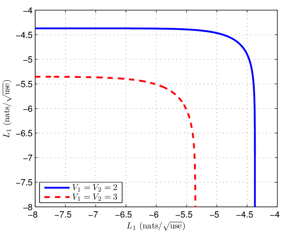
Figure 7.3: Illustration of the region $\mathcal{L}(\varepsilon;R_{1}^{*},R_{2}^{*})$ in Case (iii) with $\varepsilon=10^{-3}$. The regions are to the bottom left of the boundaries indicated.

Second, notice that for Case (iii), $\mathcal{L}(\varepsilon;R_{1}^{*},R_{2}^{*})$ is a function of $\varepsilon$ and both $V_{1}$ and $V_{2}$ as we are operating at rates near the corner point of the capacity region. Both constraints in the capacity region in (7.2) are active. We provide an intuitive reasoning for the result in (7.21). Let $\mathcal{G}_{j}$ denote the event that message $j=1,2$ is decoded correctly. The error probability criterion in (7.8) can be rewritten as

$$\Pr\big{(}\mathcal{G}_{1}\cap\mathcal{G}_{2}\big{)}\geq 1-\varepsilon.$$ (7.22)

Assuming independence of the events $\mathcal{G}_{1}$ and $\mathcal{G}_{2}$, which is generally not true in an IC because of interfering signals,

$$\Pr\big{(}\mathcal{G}_{1}\big{)}\Pr\big{(}\mathcal{G}_{2}\big{)}\geq 1-\varepsilon.$$ (7.23)

Given that the number of messages for codebook $j$ satisfies

$$M_{jn}=\big{\lfloor}\exp\big{(}nR^{*}_{j}+\sqrt{n}L_{j}+o(\sqrt{n})\big{)}\big{\rfloor},$$ (7.24)

the optimum probability of correct detection satisfies (cf. Theorem 4.4)

$$\Pr\big{(}\mathcal{G}_{j}\big{)}=\Phi\bigg{(}-\frac{L_{j}}{\sqrt{V_{j}}}\bigg{)}+o(1)$$ (7.25)

which then (heuristically) justifies (7.21). The proof makes the steps from (7.22)–(7.25) rigorous. Since $V_{1}$ and $V_{2}$ are the dispersions of the Gaussian channels without interference, this is the second-order analogue of Carleial’s result for Gaussian ICs in the VSI regime [22] because the dispersions are not affected. Note that no cross dispersion terms are present in (7.21) unlike the Slepian-Wolf problem, where the correlation of two different entropy densities appears in the characterization of $\mathcal{L}(\varepsilon;R_{1}^{*},R_{2}^{*})$ for corner points $(R_{1}^{*},R_{2}^{*})$.

Finally, it is somewhat surprising that in the converse, even though we must ensure that the codewords $X_{1}^{n}$ and $X_{2}^{n}$ are independent, we do not need to leverage the wringing technique invented by Ahlswede [3], which was used to prove that the discrete memoryless MAC admits a strong converse. This is thanks to Gaussianity which allows us to show that the first- and second-order statistics of a certain set of information densities in (7.29)–(7.30) are independent of $\mathbf{x}_{1}$ and $\mathbf{x}_{2}$ belonging to their respective power spheres.

7.3 Proof Sketch of the Main Result

The proof of Theorem 7.1 is somewhat long and tedious so we only sketch the key steps and refer the reader to [103] for the detailed calculations.

Proof.

We begin with the converse. We may assume, using the same argument as that for the point-to-point AWGN channel (cf. the Yaglom map trick [28, Ch. 9, Thm. 6] in the proof of Theorem 4.4) that all the codewords $\mathbf{x}_{j}(m_{j})$ satisfy $\|\mathbf{x}_{j}(m_{j})\|_{2}^{2}=nS_{j},j=1,2$. Choose the auxiliary output distributions in Proposition 7.2 to be the $n$-fold products of

$$Q_{Y_{1}|X_{2}}(y_{1}|x_{2}) :=\mathcal{N}(y_{1};g_{12}x_{2},g_{11}^{2}S_{1}+1),\quad\mbox{and}$$ (7.26)

$$Q_{Y_{2}|X_{1}}(y_{2}|x_{1}) :=\mathcal{N}(y_{2};g_{21}x_{1},g_{22}^{2}S_{2}+1).$$ (7.27)

These are the output distributions induced if the input distributions $\tilde{P}_{X_{1}^{n}}$ and $\tilde{P}_{X_{2}^{n}}$ are $n$-fold products of $\mathcal{N}(0,S_{1})$ and $\mathcal{N}(0,S_{2})$ respectively. Fix any achievable $(\varepsilon,R_{1}^{*},R_{2}^{*})$-second-order coding rate pair $(L_{1},L_{2})$, i.e., $(L_{1},L_{2})\in\mathcal{L}(\varepsilon;R_{1}^{*},R_{2}^{*})$. Then, for every $\xi>0$, every sequence of $(n,M_{1n},M_{2n},S_{1},S_{2},\varepsilon_{n})$-codes satisfies

$$\log M_{jn}\geq nR_{j}^{*}+\sqrt{n}(L_{j}-\xi),\quad j=1,2,$$ (7.28)

for $n$ large enough. To keep our notation succinct, define the information densities

$$j_{1}(\mathbf{x}_{1},\mathbf{x}_{2},Y_{1}^{n}) \!:=\!\log\frac{W_{1}^{n}(Y_{1}^{n}|\mathbf{x}_{1},\mathbf{x}_{2})}{Q_{Y_{1}^{n}|X_{2}^{n}}(Y_{1}^{n}|\mathbf{x}_{2})}\!=\!\sum_{i=1}^{n}\log\frac{W_{1}(Y_{1i}|x_{1i},x_{2i})}{Q_{Y_{1}|X_{2}}(Y_{1i}|x_{2i})},\quad\mbox{and}$$ (7.29)

$$j_{2}(\mathbf{x}_{1},\mathbf{x}_{2},Y_{2}^{n}) \!:=\!\log\frac{W_{2}^{n}(Y_{2}^{n}|\mathbf{x}_{1},\mathbf{x}_{2})}{Q_{Y_{2}^{n}|X_{1}^{n}}(Y_{2}^{n}|\mathbf{x}_{1})}\!=\!\sum_{i=1}^{n}\log\frac{W_{2}(Y_{2i}|x_{1i},x_{2i})}{Q_{Y_{2}|X_{1}}(Y_{2i}|x_{1i})}.$$ (7.30)

Let $C_{j}:=\mathsf{C}(\mathsf{snr}_{j})$ for $j=1,2$. For any pair of vectors $(\mathbf{x}_{1},\mathbf{x}_{2})$ satisfying $\|\mathbf{x}_{j}\|_{2}^{2}=nS_{j}$,

$$\mathsf{E}\begin{bmatrix}j_{1}(\mathbf{x}_{1},\mathbf{x}_{2},Y_{1}^{n})\\ j_{2}(\mathbf{x}_{1},\mathbf{x}_{2},Y_{2}^{n})\end{bmatrix} =n\begin{bmatrix}C_{1}\\ C_{2}\end{bmatrix},\quad\mbox{and}$$ (7.31)

$$\operatorname{\mathsf{Cov}}\begin{bmatrix}j_{1}(\mathbf{x}_{1},\mathbf{x}_{2},Y_{1}^{n})\\ j_{2}(\mathbf{x}_{1},\mathbf{x}_{2},Y_{2}^{n})\end{bmatrix} =n\begin{bmatrix}V_{1}&0\\ 0&V_{2}\end{bmatrix}.$$ (7.32)

Importantly, notice that the covariance matrix in (7.32) is diagonal. This is due to the independence of the noises $Z_{1i}$ and $Z_{2i}$ and is the crux of the converse proof for the corner point case in (7.21).

Now let $\gamma:=n^{-3/4}$ in the probability in the non-asymptotic converse bound in (7.16). We denote this probability as $\mathfrak{p}$. By the law of total probability, the complementary probability $1-\mathfrak{p}$ can be written as

$$1\!-\!\mathfrak{p}\!=\!\int\!\Pr\Bigg{(}\begin{bmatrix}j_{1}(\mathbf{x}_{1},\mathbf{x}_{2},Y_{1}^{n})\\ j_{2}(\mathbf{x}_{1},\mathbf{x}_{2},Y_{2}^{n})\end{bmatrix}\!>\!\begin{bmatrix}\log M_{1n}\!-\!n^{1/4}\\ \log M_{2n}\!-\!n^{1/4}\end{bmatrix}\Bigg{)}\,\mathrm{d}P_{X_{1}^{n}}(\mathbf{x}_{1})\,\mathrm{d}P_{X_{2}^{n}}(\mathbf{x}_{2}).$$ (7.33)

By (7.28), for large enough $n$, the inner probability evaluates to

$$\Pr\Bigg{(}\begin{bmatrix}j_{1}(\mathbf{x}_{1},\mathbf{x}_{2},Y_{1}^{n})\\ j_{2}(\mathbf{x}_{1},\mathbf{x}_{2},Y_{2}^{n})\end{bmatrix}>\begin{bmatrix}\log M_{1n}-n^{1/4}\\ \log M_{2n}-n^{1/4}\end{bmatrix}\Bigg{)}$$

$$\leq\Pr\Bigg{(}\!\begin{bmatrix}j_{1}(\mathbf{x}_{1},\mathbf{x}_{2},Y_{1}^{n})\\ j_{2}(\mathbf{x}_{1},\mathbf{x}_{2},Y_{2}^{n})\end{bmatrix}>\begin{bmatrix}nR_{1}^{*}-\sqrt{n}(L_{1}-2\xi)\\ nR_{2}^{*}-\sqrt{n}(L_{2}-2\xi)\end{bmatrix}\!\Bigg{)}$$ (7.34)

$$\leq\Psi\Bigg{(}\begin{bmatrix}\sqrt{n}(C_{1}-R_{1}^{*})-L_{1}+2\xi\\ \sqrt{n}(C_{2}-R_{2}^{*})-L_{2}+2\xi\end{bmatrix};\mathbf{0},\begin{bmatrix}V_{1}&0\\ 0&V_{2}\end{bmatrix}\Bigg{)}+\frac{\kappa}{\sqrt{n}}$$ (7.35)

$$=\prod_{j=1}^{2}\Phi\bigg{(}\frac{\sqrt{n}(C_{j}-R_{j}^{*})-L_{j}+2\xi}{\sqrt{V_{j}}}\bigg{)}+\frac{\kappa}{\sqrt{n}},$$ (7.36)

where (7.35) is an application of the multivariate Berry-Esseen theorem (Corollary 1.1) and $\kappa$ is a finite constant. Note that $\Psi$ denotes the bivariate generalization of the Gaussian cdf, defined in (6.11). Equality (7.36) holds because the covariance matrix in (7.35) is diagonal by the calculation in (7.32). Since the bound in (7.36) does not depend on $\mathbf{x}_{1},\mathbf{x}_{2}$ as long as $\|\mathbf{x}_{j}\|_{2}^{2}=nS_{j}$, we have

$$1-\mathfrak{p}\leq\prod_{j=1}^{2}\Phi\bigg{(}\frac{\sqrt{n}(C_{j}-R_{j}^{*})-L_{j}+2\xi}{\sqrt{V_{j}}}\bigg{)}+\frac{\kappa}{\sqrt{n}},$$ (7.37)

In Case (i), $R_{1}^{*}=C_{1}$ and $R_{2}^{*}<C_{2}$ so the term corresponding to $j=2$ in the above product converges to one and we have

$$1-\mathfrak{p}\leq\Phi\bigg{(}\frac{-L_{1}+2\xi}{\sqrt{V_{j}}}\bigg{)}+\delta_{n},$$ (7.38)

where $\delta_{n}\to 0$ as $n\to\infty$. Thus Proposition 7.2 yields

$$\varepsilon_{n}\geq\Phi\bigg{(}\frac{L_{1}-2\xi}{\sqrt{V_{j}}}\bigg{)}+\delta_{n}.$$ (7.39)

Taking $\limsup$ on both sides yields

$$\limsup_{n\to\infty}\varepsilon_{n}\geq\Phi\bigg{(}\frac{L_{1}-2\xi}{\sqrt{V_{j}}}\bigg{)}.$$ (7.40)

Since $\limsup_{n\to\infty}\varepsilon_{n}\leq\varepsilon$, we can write

$$L_{1}\leq\sqrt{V_{1}}\Phi^{-1}(\varepsilon)+2\xi.$$ (7.41)

Since $\xi>0$ is arbitrarily small, we may take $\xi\downarrow 0$ to complete the proof of the converse part for Case (i). For Case (ii), swap the indices $1$ and $2$ in the above calculation. For Case (iii), the analysis until (7.36) applies. However, now $R_{j}^{*}=C_{j}$ for both $j=1,2$ so both $\Phi(\cdot)$ functions in (7.36) are numbers strictly between $0$ and $1$. Consequently, we have

$$1-\mathfrak{p}\leq\Phi\bigg{(}\frac{-L_{1}+2\xi}{\sqrt{V_{j}}}\bigg{)}\Phi\bigg{(}\frac{-L_{2}+2\xi}{\sqrt{V_{2}}}\bigg{)}+\frac{\kappa}{\sqrt{n}}.$$ (7.42)

The rest of the arguments are similar to those for Case (i).

For the direct part, similarly to the single-user case in (4.94), we choose the input distributions

$$P_{X_{j}^{n}}(\mathbf{x}_{j})=\frac{\delta\{\|\mathbf{x}_{j}\|_{2}^{2}-nS_{j}\}}{A_{n}(\sqrt{nS_{j}})},\qquad j=1,2,$$ (7.43)

where $\delta\{\cdot\}$ is the Dirac $\delta$-function and $A_{n}(r)$ is the area of a sphere in $\mathbb{R}^{n}$ with radius $r$. Clearly, the power constraints are satisfied with probability one. We choose the conditional output distributions $Q_{Y_{1}^{n}|X_{2}^{n}}$ and $Q_{Y_{2}^{n}|X_{1}^{n}}$ as in (7.26) and (7.27) and the output distributions $Q_{Y_{1}^{n}}$ and $Q_{Y_{2}^{n}}$ to be the $n$-fold products of

$$Q_{Y_{1}}(y_{1}) :=\mathcal{N}(y_{1};0,g_{11}^{2}S_{1}+g_{12}^{2}S_{2}+1),\quad\mbox{and}$$ (7.44)

$$Q_{Y_{2}}(y_{2}) :=\mathcal{N}(y_{2};0,g_{21}^{2}S_{1}+g_{22}^{2}S_{2}+1).$$ (7.45)

With these choices of auxiliary output distributions, one can show the following technical lemma concerning the ratios of the induced (conditional) output distributions and the chosen (conditional) output distributions in Proposition 7.1. This is the multi-terminal analogue of (4.114) for the point-to-point AWGN channel and it allows us to replace the inconvenient induced output distributions $P_{X_{1}^{n}}W_{1}^{n}$ and $P_{X_{1}^{n}}P_{X_{2}^{n}}W_{1}^{n}$ (which is present in standard Feinstein-type achievability bounds, for example [66]) with the convenient $Q_{Y_{1}^{n}|X_{2}^{n}}$ and $Q_{Y_{1}^{n}}$ without too much degradation in error probability.

Lemma 7.1.

Let $Q_{Y_{1}^{n}},Q_{Y_{2}^{n}},Q_{Y_{1}^{n}|X_{2}^{n}}$ and $Q_{Y_{2}^{n}|X_{1}^{n}}$ be defined as the $n$-fold products of those in (7.44), (7.45), (7.26) and (7.27) respectively. Then, there exists a finite constant $\bar{\zeta}$ such that the ratios $\zeta_{jk}$ in (7.14)–(7.15) are uniformly bounded by $\bar{\zeta}$ as $n$ grows. Hence, their sum $\zeta=\sum_{j,k=1}^{2}\zeta_{jk}$ is also uniformly bounded.

The proof of this lemma can be found in [103] and [112].

Because $X_{1}^{n}$ and $X_{2}^{n}$ are uniform on their respective power spheres, it is not straightforward to analyze the behavior of random vector

$$\mathbf{B}=\begin{bmatrix}B_{11}\\ B_{21}\\ B_{12}\\ B_{22}\end{bmatrix}:=\begin{bmatrix}\log\frac{W_{1}^{n}(Y_{1}^{n}|X_{1}^{n},X_{2}^{n})}{Q_{Y_{1}^{n}|X_{2}^{n}}(Y_{1}^{n}|X_{2}^{n})}\\ \log\frac{W_{2}^{n}(Y_{2}^{n}|X_{1}^{n},X_{2}^{n})}{Q_{Y_{2}^{n}|X_{1}^{n}}(Y_{2}^{n}|X_{1}^{n})}\\ \log\frac{W_{1}^{n}(Y_{1}^{n}|X_{1}^{n},X_{2}^{n})}{Q_{Y_{1}^{n}}(Y_{1}^{n})}\\ \log\frac{W_{2}^{n}(Y_{2}^{n}|X_{1}^{n},X_{2}^{n})}{Q_{Y_{2}^{n}}(Y_{2}^{n})}\end{bmatrix},$$ (7.46)

which is present in (7.13). Note that $\mathbf{B}$ can be written as a sum of dependent random variables due to the product structure of the chosen output distributions. To analyze the probabilistic behavior of $\mathbf{B}$ for large $n$, we leverage a technique by MolavianJazi and Laneman [112]. The basic ideas are as follows: Let $T_{j}^{n}\sim\mathcal{N}(\mathbf{0}_{n},\mathbf{I}_{n\times n})$ for $j=1,2$ be standard Gaussian random vectors that are independent of each other and of the noises $Z^{n}_{j}$. Note that the input distributions in (7.43) allow us to write $X_{ji}$ as

$$X_{ji}=\sqrt{nS_{j}}\frac{T_{ji}}{\|T_{j}^{n}\|_{2}},\qquad i=1,\ldots,n.$$ (7.47)

Indeed, $\|X_{j}^{n}\|_{2}^{2}=nS_{j}$ with probability one from the random code construction and (7.47). Now consider the length-$10$ random vector $\mathbf{U}_{i}:=(\{U_{j1i}\}_{j=1}^{4},\{U_{j2i}\}_{j=1}^{4},U_{9i},U_{10i})$, where

$$U_{11i}:=1-Z_{1i}^{2},\quad U_{21i}:=g_{11}\sqrt{S_{1}}T_{1i}Z_{1i},\,$$ (7.48)

$$U_{31i}:=g_{12}\sqrt{S_{2}}T_{2i}Z_{1i},\quad U_{41i}:=g_{11}g_{12}\sqrt{S_{1}S_{2}}T_{1i}T_{2i},\,$$ (7.49)

$$U_{12i}:=1-Z_{2i}^{2},\quad U_{22i}:=g_{22}\sqrt{S_{2}}T_{2i}Z_{2i},\,$$ (7.50)

$$U_{32i}:=g_{21}\sqrt{S_{1}}T_{1i}Z_{2i},\quad U_{42i}:=g_{21}g_{22}\sqrt{S_{1}S_{2}}T_{1i}T_{2i},\,$$ (7.51)

$$U_{9i}:=T_{1i}^{2}-1,\quad U_{10i}:=T_{2i}^{2}-1.$$ (7.52)

Clearly, $\mathbf{U}_{i}$ is i.i.d. across channel uses. Furthermore, $\mathsf{E}[\mathbf{U}_{1}]=\mathbf{0}$ and $\mathsf{E}[\|\mathbf{U}_{1}\|_{2}^{3}]$ is finite. The covariance matrix of $\mathbf{U}_{1}$ can also be computed. Define the functions $\tau_{11},\tau_{12}:\mathbb{R}^{10}\to\mathbb{R}$

$$\tau_{11}(\mathbf{u}) :=\mathsf{snr}_{1}\,u_{11}+\frac{2u_{21}}{\sqrt{1+u_{9}}},\quad\mbox{and}$$ (7.53)

$$\tau_{12}(\mathbf{u}) :=(\mathsf{snr}_{1}+\mathsf{inr}_{1})u_{11}+\frac{2u_{21}}{\sqrt{1+u_{9}}}+\frac{2u_{31}}{\sqrt{1+u_{10}}}$$

$$\qquad+\frac{2u_{41}}{\sqrt{1+u_{9}}\sqrt{1+u_{10}}},$$ (7.54)

for user $1$, and analogously for user $2$. Then, through some algebra, one sees that $B_{11}$ and $B_{12}$ can be written as

$$B_{11} =n\mathsf{C}(\mathsf{snr}_{1})+\frac{n}{2(1+\mathsf{snr}_{1})}\,\tau_{11}\bigg{(}\frac{1}{n}\sum_{i=1}^{n}\mathbf{U}_{i}\bigg{)},\quad\mbox{and}$$ (7.55)

$$B_{12} =n\mathsf{C}(\mathsf{snr}_{1}+\mathsf{inr}_{1})+\frac{n}{2(1+\mathsf{snr}_{1}+\mathsf{inr}_{1})}\,\tau_{12}\bigg{(}\frac{1}{n}\sum_{i=1}^{n}\mathbf{U}_{i}\bigg{)}.$$ (7.56)

The other random variables in the $\mathbf{B}$ vector can be expressed similarly.

From (7.55)–(7.56), we are able to see the essence of the MolavianJazi-Laneman [112] technique. The information densities $B_{jk},j,k=1,2$ were initially difficult to analyze because the input random vectors $X_{j}^{n}$ in (7.43) are uniform on power spheres. This choice of input distributions results in codewords $X_{j}^{n}$ whose coordinates are dependent so standard limit theorems do not readily apply. By defining higher-dimensional random vectors $\mathbf{U}_{i}$ and appropriate functions $\tau_{jk}$, one then sees that $\mathbf{B}$ can be expressed as a function of a sum of i.i.d. random vectors. Now, one may consider a Taylor expansion of the differentiable functions $\tau_{jk}$ around the mean $\mathbf{0}$ to approximate $\mathbf{B}$ with a sum of i.i.d. random vectors. Through this analysis, one can rigorously show that

$$\frac{1}{\sqrt{n}}\left(\mathbf{B}-n\begin{bmatrix}\mathsf{C}(\mathsf{snr}_{1})\\ \mathsf{C}(\mathsf{snr}_{2})\\ \mathsf{C}(\mathsf{snr}_{1}+\mathsf{inr}_{1})\\ \mathsf{C}(\mathsf{snr}_{2}+\mathsf{inr}_{2})\end{bmatrix}\right)\stackrel{{\scriptstyle\mathrm{d}}}{{\longrightarrow}}\mathcal{N}\left(\mathbf{0},\begin{bmatrix}V_{1}&0&*&*\\ 0&V_{2}&*&*\\ *&*&*&*\\ *&*&*&*\end{bmatrix}\right),$$ (7.57)

where the entries marked as $*$ are finite and inconsequential for the subsequent analyses. Recall also that $V_{j}=\mathsf{V}(\mathsf{snr}_{j})$ for $j=1,2$. In fact, the rate of convergence to Gaussianity in (7.57) can be quantified by means of Theorem 1.5.

With these preparations, we are ready to evaluate the probability in the direct bound in (7.13), which we denote as $\mathfrak{p}$. We consider all three cases in tandem. Fix $(L_{1},L_{2})\in\mathcal{L}(\varepsilon;R_{1}^{*},R_{2}^{*})$. Let the number of codewords in the $j^{\mathrm{th}}$ codebook be

$$M_{jn}=\lfloor\exp\big{(}nR_{j}^{*}+\sqrt{n}L_{j}-2n^{1/4}\big{)}\rfloor$$ (7.58)

for $j=1,2$. It is clear that

$$\liminf_{n\to\infty}\frac{1}{\sqrt{n}}\big{(}\log M_{jn}-nR_{j}^{*}\big{)}\geq L_{j}.$$ (7.59)

Also let $\gamma:=n^{-3/4}$. With these choices, the complementary probability $1-\mathfrak{p}$ can be expressed as

$$1-\mathfrak{p}=\Pr\left(\mathbf{B}>\begin{bmatrix}nR_{1}^{*}+\sqrt{n}L_{1}-n^{1/4}\\ nR_{2}^{*}+\sqrt{n}L_{2}-n^{1/4}\\ n(R_{1}^{*}+R_{2}^{*})+\sqrt{n}(L_{1}+L_{2})-3n^{1/4}\\ n(R_{1}^{*}+R_{2}^{*})+\sqrt{n}(L_{1}+L_{2})-3n^{1/4}\end{bmatrix}\right).$$ (7.60)

Now by the SVSI assumption in (7.11)–(7.12),

$$R_{1}^{*}+R_{2}^{*}\leq\mathsf{C}(\mathsf{snr}_{1})+\mathsf{C}(\mathsf{snr}_{2})<\min\{\mathsf{C}(\mathsf{snr}_{1}+\mathsf{inr}_{1}),\mathsf{C}(\mathsf{snr}_{2}+\mathsf{inr}_{2})\}.$$ (7.61)

The convergence in (7.57) implies that

$$\mathsf{E}[B_{12}]=n\mathsf{C}(\mathsf{snr}_{1}+\mathsf{inr}_{1}),\quad\mbox{and}\quad\mathsf{E}[B_{22}]=n\mathsf{C}(\mathsf{snr}_{2}+\mathsf{inr}_{2}).$$ (7.62)

Since the expectations of $B_{12}$ and $B_{22}$ are strictly larger than $R_{1}^{*}+R_{2}^{*}$ (cf. (7.61)), by standard Chernoff bounding techniques,

$$\Pr\big{(}B_{12}\!\leq\!n(R_{1}^{*}\!+\!R_{2}^{*})\!+\!\sqrt{n}(L_{1}\!+\!L_{2})\!-\!3n^{1/4}\big{)} \!\leq\!\exp(-n\xi),\,\,\mbox{and}$$ (7.63)

$$\Pr\big{(}B_{22}\!\leq\!n(R_{1}^{*}\!+\!R_{2}^{*})\!+\!\sqrt{n}(L_{1}\!+\!L_{2})\!-\!3n^{1/4}\big{)} \!\leq\!\exp(-n\xi),$$ (7.64)

for some $\xi>0$. Consequently, by the union bound, (7.60) reduces to

$$1-\mathfrak{p}\geq\Pr\left(\begin{bmatrix}B_{11}\\ B_{21}\end{bmatrix}>\begin{bmatrix}nR_{1}^{*}+\sqrt{n}L_{1}-n^{1/4}\\ nR_{2}^{*}+\sqrt{n}L_{2}-n^{1/4}\end{bmatrix}\right)-2\exp(-n\xi).$$ (7.65)

Just as in the converse, one can then analyze this probability for the various cases using the convergence to Gaussianity in (7.57). This completes the proof of the direct part. ∎

Chapter 8 A Special Class of Gaussian Multiple Access Channels

The multiple access channel (MAC) is a communication model in which many parties would like to simultaneously send independent messages over a common medium to a sole destination. Together with the broadcast, interference and relay channels, the MAC is a fundamental building block of more complicated communication networks. For example, the MAC is an appropriate model for the uplink of cellular systems where multiple mobile phone users would like to communicate to a distant base station over a wireless medium. The capacity region of the MAC is, by now, well known and goes back to the work by Ahlswede [1] and Liao [105] in the early 1970s. The strong converse was established by Dueck [47] and Ahlswede [3].

A yet simpler model, which we consider in this chapter, is the asymmetric MAC (A-MAC) as shown in Fig. 8.1. This channel model, also known as the MAC with degraded message sets [49, Ex. 5.18(b)] or the cognitive [44] MAC, was first studied by Haroutunian [72], Prelov [128] and van der Meulen [167]. Here, encoder $1$ has knowledge of both messages $m_{1}$ and $m_{2}$, while encoder $2$ only has its own message $m_{2}$. For the Gaussian case, the channel law is $Y=X_{1}+X_{2}+Z$, where $Z$ is standard Gaussian noise. The capacity region [49, Ex. 5.18(b)] is the set of all $(R_{1},R_{2})$ satisfying

$$R_{1}\leq\mathsf{C}\big{(}(1-\rho^{2})S_{1}\big{)},\quad\mbox{and}\quad R_{1}+R_{2}\leq\mathsf{C}\big{(}S_{1}+S_{2}+2\rho\sqrt{S_{1}S_{2}}\big{)}$$ (8.1)

for some $\rho\in[0,1]$ where $S_{1}$ and $S_{2}$ are the admissible transmit powers. Rate pairs in (8.1) are achieved using superposition coding [31]. This region for $S_{1}=S_{2}=1$ is shown in Fig. 8.2. Observe that $\rho\in[0,1]$ parametrizes points on the boundary. Each point on the curved part of the boundary is achieved by a unique bivariate Gaussian distribution.

Figure 8.1: Illustration of the asymmetric MAC or A-MAC

\begin{overpic}[width=314.37714pt]{gauss_mac.pdf} \put(80.0,23.0){\circle*{2.0}} \put(82.0,23.0){(i)} \put(9.0,96.0){(iii)} \put(55.0,66.0){(ii)} \put(55.0,63.0){\circle*{2.0}} \put(10.0,94.0){\circle*{2.0}} \put(40.0,48.0){\vector(1,1){15.0}} \put(65.0,42.5){\vector(-1,2){10.0}} \put(38.0,45.0){\mbox{$\mathbf{v}$}} \put(65.0,39.5){\mbox{$\mathbf{v}^{\prime}$}} \end{overpic}

Figure 8.2: Capacity region of a Gaussian A-MAC where $S_{1}=S_{2}=1$. The three cases of Theorem 8.1 are illustrated. Each $\rho\in(0,1]$ corresponds to a trapezoid of rate pairs achievable by a unique input distribution $\mathcal{N}(\mathbf{0},\bm{\Sigma}(\rho))$. However, coding with a fixed input distribution is insufficient to achieve all angles of approach to a boundary point as there are regions within $\mathcal{C}$ not in the trapezoid parametrized by $\rho$. Suppose $\rho=\frac{2}{3}$, one can approach the corner point in the direction indicated by the vector $\mathbf{v}$ using the fixed input distribution $\mathcal{N}(\mathbf{0},\bm{\Sigma}(\frac{2}{3}))$, but the same is not true of the direction indicated by $\mathbf{v}^{\prime}$, since the approach is from outside the trapezoid.

In this chapter, we show that the assumptions concerning Gaussianity and asymmetry of the messages sets (i.e., partial cooperation) allow us to determine the second-order asymptotics of this model. The main result here is of a somewhat different flavor compared to results in previous chapters on multi-terminal information theory problems because the second-order rate region $\mathcal{L}(\varepsilon;R_{1}^{*},R_{2}^{*})$ is characterized not only in terms of covariances of vectors of information densities or dispersions. Indeed, we will see that there is a subtle interaction between the derivatives of the first-order capacity terms in (8.1) with respect to $\rho$, and the dispersions in the description of $\mathcal{L}(\varepsilon;R_{1}^{*},R_{2}^{*})$. The fact that the derivatives appear in the answer to an information-theoretic question appears to be novel. The difference in the characterization of $\mathcal{L}(\varepsilon;R_{1}^{*},R_{2}^{*})$ compared to second-order regions in previous chapters is because, with the union over $\rho\in[0,1]$, the boundary of the capacity region in (8.1) is curved in contrast to the polygonal capacity regions in previous chapters. We will see that the curvature of the boundary results in the second-order region $\mathcal{L}(\varepsilon;R_{1}^{*},R_{2}^{*})$ being a half-space in $\mathbb{R}^{2}$. This half-space is characterized by a slope and intercept, both of which are expressible in terms of the dispersions, together with the derivatives of the capacities.

Intuitively, the extra derivative term arises because we need to account for all possible angles of approach to a boundary point $(R_{1}^{*},R_{2}^{*})$. Using a sequence of input distributions parametrized by a single correlation parameter $\rho$ not depending on the blocklength turns out to be suboptimal in the second-order sense, as we can only achieve the angles of approach within the specific trapezoid parametrized by $\rho$ (see Fig. 8.2 and its caption). Thus, our coding strategy is to let the sequence of input distributions vary with the blocklength. In particular, they are parametrized by a sequence $\{\rho_{n}\}_{n\in\mathbb{N}}$ that converges to $\rho$ with speed $\Theta(\frac{1}{\sqrt{n}})$. A Taylor expansion of the first-order capacity vector then yields the derivative term.

Similarly to the Gaussian IC with SVSI, the achievability proof uses the coding on spheres strategy in which pairs of codewords are drawn uniformly at random from high-dimensional spheres. However, because the underlying coding strategy involves superposition coding, the analysis is more subtle. In particular, we are required to bound the ratios of certain induced output densities and product output densities. The proof of the converse part involves several new ideas including (i) reduction to almost constant correlation type subcodes; (ii) evaluation of a global outer bound and (iii) specialization of the global outer bound to obtain local second-order asymptotic results.

The material in this chapter is based on work by Scarlett and Tan [138].

8.1 Definitions and Non-Asymptotic Bounds

The model we consider is as follows:

$$Y_{i}=X_{1i}+X_{2i}+Z_{i}$$ (8.2)

where $i=1,\ldots,n$ and $Z_{i}\sim\mathcal{N}(0,1)$ is white Gaussian noise. The channel gains are set to unity without loss of generality. Thus, the channel transition law is

$$W(y|x_{1},x_{2})=\frac{1}{\sqrt{2\pi}}\exp\left(-\frac{1}{2}(y-x_{1}-x_{2})^{2}\right).$$ (8.3)

The channel operates in a stationary and memoryless manner.

We define an $(n,M_{1},M_{2},S_{1},S_{2},\varepsilon)$-code for the Gaussian A-MAC which includes two encoders $f_{1}:\{1,\ldots,M_{1}\}\times\{1,\ldots,M_{2}\}\to\mathbb{R}^{n}$, $f_{2}:\{1,\ldots,M_{2}\}\to\mathbb{R}^{n}$ and a decoder $\varphi:\mathbb{R}^{n}\to\{1,\ldots,M_{1}\}\times\{1,\ldots,M_{2}\}$ such that the following power constraints are satisfied

$$\big{\|}f_{1}(m_{1},m_{2})\big{\|}_{2}^{2}=\sum_{i=1}^{n}f_{1i}(m_{1})^{2} \leq nS_{1},\quad\mbox{and}$$ (8.4)

$$\big{\|}f_{2}(m_{2})\big{\|}_{2}^{2}=\sum_{i=1}^{n}f_{2i}(m_{2})^{2} \leq nS_{2},$$ (8.5)

and the average error probability

$$\frac{1}{M_{1}M_{2}}\sum_{m_{1}=1}^{M_{1}}\sum_{m_{2}=1}^{M_{2}}W^{n}\big{(}\mathbb{R}^{n}\!\times\!\mathbb{R}^{n}\setminus\mathcal{D}_{m_{1},m_{2}}\big{|}f_{1}(m_{1},m_{2}),f_{2}(m_{2})\big{)}\!\leq\!\varepsilon.$$ (8.6)

As with the Gaussian IC discussed in the previous chapter, $\mathcal{D}_{m_{1},m_{2}}$ denotes the decoding region for messages $(m_{1},m_{2})$ and $S_{j}$ represents the admissible power for the $j^{\mathrm{th}}$ user.

The following non-asymptotic bounds are easily derived. They are analogues of the bounds by Feinstein [53] and Verdú-Han [169] (or Hayashi-Nagaoka [77]). See Boucheron-Salamatian [20] for the proofs of similar results.

Proposition 8.1 (Achievability bound for the A-MAC).

Fix any input joint distribution $P_{X_{1}^{n}X_{2}^{n}}$ whose support satisfies the power constraints in (8.4)–(8.5), i.e., $\|X_{j}^{n}\|_{2}\leq nS_{j}$ with probability one. For every $n\in\mathbb{N}$, every $\gamma>0$, any choice of output distributions $Q_{Y^{n}|X_{2}^{n}}$ and $Q_{Y^{n}}$, and any two sets $\mathcal{A}_{1}\subset\mathcal{X}_{2}^{n}\times\mathcal{Y}^{n}$ and $\mathcal{A}_{12}\subset\mathcal{Y}^{n}$, there exists an $(n,M_{1},M_{2},S_{1},S_{2},\varepsilon)$-code for the A-MAC such that

$$\varepsilon \leq\Pr\bigg{(}\log\frac{W^{n}(Y^{n}|X_{1}^{n},X_{2}^{n})}{Q_{Y^{n}|X_{2}^{n}}(Y^{n}|X_{2}^{n})}\!\leq\!\log M_{1}\!+\!n\gamma\quad\mbox{or }$$

$$\hskip 36.135pt\log\frac{W^{n}(Y^{n}|X_{1}^{n},X_{2}^{n})}{Q_{Y^{n}}(Y^{n})}\!\leq\!\log(M_{1}M_{2})\!+\!n\gamma\bigg{)}$$

$$\hskip 36.135pt+\Pr\big{(}(X_{2}^{n},Y^{n})\notin\mathcal{A}_{1}\big{)}+\Pr\big{(}Y^{n}\notin\mathcal{A}_{12}\big{)}+\zeta\exp(-n\gamma),$$ (8.7)

where $\zeta=\zeta_{1}+\zeta_{12}$ and

$$\zeta_{1} :=\sup_{(\mathbf{x}_{2},\mathbf{y})\in\mathcal{A}_{1}}\frac{P_{X_{1}^{n}|X_{2}^{n}}W^{n}(\mathbf{y}|\mathbf{x}_{2})}{Q_{Y^{n}|X_{2}^{n}}(\mathbf{y}|\mathbf{x}_{2})},\quad\zeta_{12}:=\sup_{\mathbf{y}\in\mathcal{A}_{12}}\frac{P_{X_{1}^{n}X_{2}^{n}}W^{n}(\mathbf{y})}{Q_{Y^{n}}(\mathbf{y})}.$$ (8.8)

Again notice that our freedom to choose $Q_{Y^{n}|X_{2}^{n}}$ and $Q_{Y^{n}}$ results in the need to control $\zeta_{1}$ and $\zeta_{12}$, which are the maximum values of the ratios of the densities induced by the code with respect to the chosen output densities. The maximum values are restricted to those typical values of $(\mathbf{x}_{2},\mathbf{y})$ and $\mathbf{y}$ indicated by the chosen sets $\mathcal{A}_{1}$ and $\mathcal{A}_{12}$.

Proposition 8.2 (Converse bound for the A-MAC).

For every $n\in\mathbb{N}$, every $\gamma>0$ and for any choice of output distributions $Q_{Y^{n}|X_{2}^{n}}$ and $Q_{Y^{n}}$, every $(n,M_{1},M_{2},S_{1},S_{2},\varepsilon)$-code for the A-MAC must satisfy

$$\varepsilon\geq\Pr\bigg{(}\log\frac{W^{n}(Y^{n}|X_{1}^{n},X_{2}^{n})}{Q_{Y^{n}|X_{2}^{n}}(Y^{n}|X_{2}^{n})} \!\leq\!\log M_{1}\!-\!n\gamma\quad\mbox{or }$$

$$\log\frac{W^{n}(Y^{n}|X_{1}^{n},X_{2}^{n})}{Q_{Y^{n}}(Y^{n})} \!\leq\!\log(M_{1}M_{2})\!-\!n\gamma\bigg{)}\!-\!2\exp(-n\gamma),$$ (8.9)

for some input joint distribution $P_{X_{1}^{n}X_{2}^{n}}$ whose support satisfies the power constraints in (8.4)–(8.5).

8.2 Second-Order Asymptotics

As in the previous chapters on multi-terminal problems, given a point on the boundary of the capacity region $(R_{1}^{*},R_{2}^{*})$, we are interested in characterizing the set of all $(L_{1},L_{2})$ pairs for which there exists a sequence of $(n,M_{1n},M_{2n},S_{1},S_{2},\varepsilon_{n})$-codes such that

$$\liminf_{n\to\infty}\frac{1}{\sqrt{n}}\big{(}\log M_{jn}-nR_{j}^{*}\big{)}\geq L_{j},\,\,\mbox{and}\,\,\limsup_{n\to\infty}\varepsilon_{n}\leq\varepsilon.$$ (8.10)

We denote this set as $\mathcal{L}(\varepsilon;R_{1}^{*},R_{2}^{*})\subset\mathbb{R}^{2}$.

8.2.1 Preliminary Definitions

Before we can state the main results, we need to define a few more fundamental quantities. For a pair of rates $(R_{1},R_{2})$, the rate vector is

$$\mathbf{R}:=\begin{bmatrix}R_{1}\\ R_{1}+R_{2}\end{bmatrix}.$$ (8.11)

The input distribution to achieve a point on the boundary characterized by some $\rho\in[0,1]$ is a $2$-dimensional Gaussian distribution with zero mean and covariance matrix

$$\bm{\Sigma}(\rho):=\begin{bmatrix}S_{1}&\rho\sqrt{S_{1}S_{2}}\\ \rho\sqrt{S_{1}S_{2}}&S_{2}\end{bmatrix}.$$ (8.12)

The corresponding mutual information vector is given by

$$\mathbf{I}(\rho)=\begin{bmatrix}I_{1}(\rho)\\ I_{12}(\rho)\end{bmatrix}:=\begin{bmatrix}\mathsf{C}\big{(}S_{1}(1-\rho^{2})\big{)}\\ \mathsf{C}\big{(}S_{1}+S_{2}+2\rho\sqrt{S_{1}S_{2}}\big{)}\end{bmatrix}.$$ (8.13)

Let

$$\mathsf{V}(x,y):=\log^{2}\mathrm{e}\cdot\frac{x(y+2)}{2(x+1)(y+1)}$$ (8.14)

be the Gaussian cross-dispersion function and note that $\mathsf{V}(x):=\mathsf{V}(x,x)$ is the Gaussian dispersion function defined previously in (4.85). For fixed $0\leq\rho\leq 1$, define the information-dispersion matrix

$$\mathbf{V}(\rho):=\begin{bmatrix}V_{1}(\rho)&V_{1,12}(\rho)\\ V_{1,12}(\rho)&V_{12}(\rho)\end{bmatrix},$$ (8.15)

where the elements of the matrix are

$$V_{1}(\rho) :=\mathsf{V}\big{(}S_{1}(1-\rho^{2})\big{)},$$ (8.16)

$$V_{1,12}(\rho) :=\mathsf{V}\big{(}S_{1}(1-\rho^{2}),S_{1}+S_{2}+2\rho\sqrt{S_{1}S_{2}}\big{)},$$ (8.17)

$$V_{12}(\rho) :=\mathsf{V}\big{(}S_{1}+S_{2}+2\rho\sqrt{S_{1}S_{2}}\big{)}.$$ (8.18)

Let $(X_{1},X_{2})\sim P_{X_{1}X_{2}}=\mathcal{N}(\mathbf{0},\bm{\Sigma}(\rho))$ and define $Q_{Y|X_{2}}$ and $Q_{Y}$ to be Gaussian distributions induced by $P_{X_{1}X_{2}}$ and $W$, namely

$$Q_{Y|X_{2}}(y|x_{2}) :=\mathcal{N}\big{(}y;x_{2}(1+\rho\sqrt{S_{1}/S_{2}}),1+S_{1}(1-\rho^{2})\big{)},\quad\mbox{and}$$ (8.19)

$$Q_{Y}(y) :=\mathcal{N}\big{(}y;0,1+S_{1}+S_{2}+2\rho\sqrt{S_{1}S_{2}}\big{)}.$$ (8.20)

It should be noted that the random variables $(X_{1},X_{2})$ and the densities $Q_{Y|X_{2}}$ and $Q_{Y}$ all depend on $\rho$; this dependence is suppressed throughout the chapter. The mutual information vector $\mathbf{I}(\rho)$ and information-dispersion matrix $\mathbf{V}(\rho)$ are the mean vector and conditional covariance matrix of the information density vector

$$\mathbf{j}(x_{1},x_{2},y):=\begin{bmatrix}j_{1}(x_{1},x_{2},y)\\ j_{12}(x_{1},x_{2},y)\end{bmatrix}=\begin{bmatrix}\log\frac{W(y|x_{1},x_{2})}{Q_{Y|X_{2}}(y|x_{2})}\\ \log\frac{W(y|x_{1},x_{2})}{Q_{Y}(y)}\end{bmatrix}.$$ (8.21)

That is, we can write $\mathbf{I}(\rho)$ and $\mathbf{V}(\rho)$ as

$$\mathbf{I}(\rho) =\mathsf{E}\big{[}\,\mathbf{j}(X_{1},X_{2},Y)\big{]},\quad\mbox{and}$$ (8.22)

$$\mathbf{V}(\rho) =\mathsf{E}\big{[}\operatorname{\mathsf{Cov}}\big{(}\mathbf{j}(X_{1},X_{2},Y)\,\big{|}\,X_{1},X_{2}\big{)}\big{]},$$ (8.23)

with $(X_{1},X_{2},Y)\sim P_{X_{1}X_{2}}\times W$. We also need a generalization of the $\Phi^{-1}(\cdot)$ function. Define the “inverse image” of $\Psi(z_{1},z_{2};\mathbf{0},\bm{\Sigma})$ as

$$\Psi^{-1}(\bm{\Sigma},\varepsilon):=\big{\{}(t_{1},t_{2})\in\mathbb{R}^{2}:\Psi(-z_{1},-z_{2};\mathbf{0},\bm{\Sigma})\geq 1-\varepsilon\big{\}}.$$ (8.24)

An illustration of this set is provided in Fig. 8.3. Observe that for $\varepsilon<\frac{1}{2}$, the set lies entirely within the third quadrant of the $\mathbb{R}^{2}$ plane. This represents “backoffs” from the first-order fundamental limits.

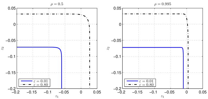
Figure 8.3: Illustration of the set $\Psi^{-1}(\mathbf{V}(\rho),\varepsilon)$ where $\mathbf{V}(\rho)$ is defined in (8.15). The regions are to the bottom left of the boundaries indicated.

8.2.2 Global Second-Order Asymptotics

Here we provide inner and outer bounds on $\mathcal{C}(n,\varepsilon)$, defined to be the set of $(R_{1},R_{2})$ pairs such that there exist codebooks of length $n$ and rates at least $R_{1}$ and $R_{2}$ yielding an average error probability not exceeding $\varepsilon$. Let $\underline{g}(\rho,\varepsilon,n)$ and $\overline{g}(\rho,\varepsilon,n)$ be arbitrary functions of $\rho$, $\varepsilon$ and $n$ for now, and define the inner and outer regions

$$\underline{\mathcal{R}}(n,\varepsilon;\rho) :=\bigg{\{}(R_{1},R_{2}):\mathbf{R}\in\mathbf{I}(\rho)+\frac{\Psi^{-1}(\mathbf{V}(\rho),\varepsilon)}{\sqrt{n}}+\underline{g}(\rho,\varepsilon,n)\mathbf{1}\bigg{\}},$$ (8.25)

$$\overline{\mathcal{R}}(n,\varepsilon;\rho) :=\bigg{\{}(R_{1},R_{2}):\mathbf{R}\in\mathbf{I}(\rho)+\frac{\Psi^{-1}(\mathbf{V}(\rho),\varepsilon)}{\sqrt{n}}+\overline{g}(\rho,\varepsilon,n)\mathbf{1}\bigg{\}}.$$ (8.26)

Lemma 8.1 (Global Bounds on the $(n,\varepsilon)$-Capacity Region).

There exist functions $\underline{g}(\rho,\varepsilon,n)$ and $\overline{g}(\rho,\varepsilon,n)$ such that

$$\bigcup_{0\leq\rho\leq 1}\underline{\mathcal{R}}(n,\varepsilon;\rho)\subset\mathcal{C}(n,\varepsilon)\subset\bigcup_{-1\leq\rho\leq 1}\overline{\mathcal{R}}(n,\varepsilon;\rho),$$ (8.27)

and $\underline{g}$ and $\overline{g}$ satisfy the following properties:
(i) For any sequence $\{\rho_{n}\}_{n\in\mathbb{N}}$ with $\rho_{n}\to\rho\in(-1,1)$, we have

$$\underline{g}(\rho_{n},\varepsilon,n)=O\left(\frac{\log n}{n}\right),\quad\mbox{and}\quad\overline{g}(\rho_{n},\varepsilon,n)=O\left(\frac{\log n}{n}\right).$$ (8.28)

(ii) Else, for any sequence $\{\rho_{n}\}_{n\in\mathbb{N}}$ with $\rho_{n}\to\pm 1$, we have

$$\underline{g}(\rho_{n},\varepsilon,n)=o\left(\frac{1}{\sqrt{n}}\right),\quad\mbox{and}\quad\overline{g}(\rho_{n},\varepsilon,n)=o\left(\frac{1}{\sqrt{n}}\right).$$ (8.29)

Lemma 8.1 serves as a stepping stone to establish the local behavior of first-order optimal codes near a boundary point. A proof sketch of the lemma is provided in Section 8.3.1.

We remark that even though the union for the outer bound in (8.27) is taken over $\rho\in[-1,1]$, only the values $\rho\in[0,1]$ will play a role in establishing the local asymptotics in Section 8.2.3, since negative values of $\rho$ are not even first-order optimal, i.e., they fail to achieve a point on the boundary of the capacity region.

We do not claim that the remainder terms in (8.28)–(8.29) are uniform in the limiting value $\rho$ of $\{\rho_{n}\}_{n\in\mathbb{N}}$; such uniformity will not be required in establishing our main local result below. On the other hand, it is crucial that values of $\rho$ varying with $n$ are handled.

8.2.3 Local Second-Order Asymptotics

To characterize $\mathcal{L}(\varepsilon;R_{1}^{*},R_{2}^{*})$, we need yet another definition, which is a feature we have not encountered thus far in this monograph. Define

$$\mathbf{D}(\rho)=\begin{bmatrix}D_{1}(\rho)\\ D_{12}(\rho)\end{bmatrix}:=\frac{\partial}{\partial\rho}\begin{bmatrix}I_{1}(\rho)\\ I_{12}(\rho)\end{bmatrix},$$ (8.30)

to be the derivative of the mutual information vector with respect to $\rho$ where the individual derivatives are given by

$$\frac{\partial I_{1}(\rho)}{\partial\rho} =\frac{-S_{1}\rho}{1+S_{1}(1-\rho^{2})},\quad\mbox{and}$$ (8.31)

$$\frac{\partial I_{12}(\rho)}{\partial\rho} =\frac{\sqrt{S_{1}S_{2}}}{1+S_{1}+S_{2}+2\rho\sqrt{S_{1}S_{2}}}.$$ (8.32)

Note that $\rho\in(0,1]$ represents the strictly concave part of the boundary (the part of the boundary where $R_{2}>0.2$ in Fig. 8.2), and in this interval we have $D_{1}(\rho)<0$ and $D_{12}(\rho)>0$.

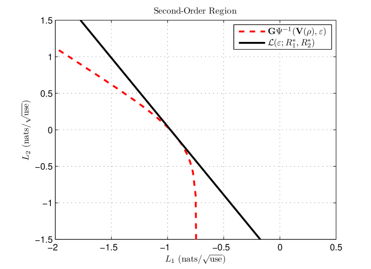
Figure 8.4: Illustration of the set $\mathcal{L}(\varepsilon;R_{1}^{*},R_{2}^{*})$ in (8.35) with $S_{1}=S_{2}=1$, $\rho=\frac{1}{2}$ and $\varepsilon=0.1$. The set corresponding to $\beta=0$ in (8.35) is denoted as $\mathbf{G}\Psi^{-1}(\mathbf{V}(\rho),\varepsilon)$. Regions are to the bottom-left of the boundaries.

Furthermore, for a vector $\mathbf{v}=(v_{1},v_{2})\in\mathbb{R}^{2}$, we define the down-set of $\mathbf{v}$ as

$$\mathbf{v}^{-}:=\{(w_{1},w_{2})\in\mathbb{R}^{2}:w_{1}\leq v_{1},w_{2}\leq v_{2}\}.$$ (8.33)

We are now in a position to state our main result whose proof is sketched in Section 8.3.2.

Theorem 8.1 (Local Second-Order Rates).

Depending on $(R_{1}^{*},R_{2}^{*})$ (see Fig. 8.2), we have the following three cases:
Case (i): $R_{1}^{*}=I_{1}(0)$ and $R_{1}^{*}+R_{2}^{*}\leq I_{12}(0)$ (vertical segment of the boundary corresponding to $\rho=0$),

$$\mathcal{L}(\varepsilon;R_{1}^{*},R_{2}^{*})=\left\{(L_{1},L_{2}):L_{1}\leq\sqrt{V_{1}(0)}\Phi^{-1}(\varepsilon)\right\}.$$ (8.34)

Case (ii): $R_{1}^{*}=I_{1}(\rho)$ and $R_{1}^{*}+R_{2}^{*}=I_{12}(\rho)$ (curved segment of the boundary corresponding to $0<\rho<1$),

$$\mathcal{L}(\varepsilon;R_{1}^{*},R_{2}^{*})\!=\!\Bigg{\{}(L_{1},L_{2}):\begin{bmatrix}L_{1}\\ L_{1}\!+\!L_{2}\end{bmatrix}\!\in\!\bigcup_{\beta\in\mathbb{R}}\Big{\{}\beta\,\mathbf{D}(\rho)\!+\!\Psi^{-1}(\mathbf{V}(\rho),\varepsilon)\Big{\}}\Bigg{\}}.$$ (8.35)

Case (iii): $R_{1}^{*}=0$ and $R_{1}^{*}+R_{2}^{*}=I_{12}(1)$ (point on the vertical axis corresponding to $\rho=1$),

$$\mathcal{L}(\varepsilon;R_{1}^{*},R_{2}^{*})$$

$$=\Bigg{\{}(L_{1},L_{2}):\begin{bmatrix}L_{1}\\ L_{1}+L_{2}\end{bmatrix}\!\in\!\bigcup_{\beta\leq 0}\bigg{\{}\beta\,\mathbf{D}(1)+\begin{bmatrix}0\\ \sqrt{V_{12}(1)}\Phi^{-1}(\varepsilon)\end{bmatrix}^{-}\bigg{\}}\Bigg{\}}.$$ (8.36)

See Fig. 8.4 for an illustration of $\mathcal{L}(\varepsilon;R_{1}^{*},R_{2}^{*})$ in (8.35) and the set of $(L_{1},L_{2})$ such that $(L_{1},L_{1}+L_{2})$ belongs to $\Psi^{-1}(\mathbf{V}(\rho),\varepsilon)$, i.e., $\mathbf{G}\Psi^{-1}(\mathbf{V}(\rho),\varepsilon)$, where $\mathbf{G}=[1,0;-1,1]$ is the invertible matrix that transforms the coordinate system from $[L_{1},L_{1}+L_{2}]^{\prime}$ to $[L_{1},L_{2}]^{\prime}$. In other words, $\mathbf{G}\Psi^{-1}(\mathbf{V}(\rho),\varepsilon)$ is the same set as that in (8.35) neglecting the union and setting $\beta=0$. It can be seen that $\mathbf{G}\Psi^{-1}(\mathbf{V}(\rho),\varepsilon)$ is a strict subset of $\mathcal{L}(\varepsilon;R_{1}^{*},R_{2}^{*})$. In fact, $\mathcal{L}(\varepsilon;R_{1}^{*},R_{2}^{*})$ is a half-space in $\mathbb{R}^{2}$ for any $(R_{1}^{*},R_{2}^{*})$ on the boundary of the capacity region corresponding to $\rho<1$. So $\mathcal{L}(\varepsilon;R_{1}^{*},R_{2}^{*})$ in (8.35) can be alternatively written as

$$\mathcal{L}(\varepsilon;R_{1}^{*},R_{2}^{*})=\big{\{}(L_{1},L_{2}):L_{2}\leq a_{\rho}L_{1}+b_{\rho,\varepsilon}\big{\}}$$ (8.37)

where the slope and intercept are respectively defined as

$$a_{\rho} :=\frac{D_{12}(\rho)-D_{1}(\rho)}{D_{1}(\rho)},\quad\mbox{and}$$ (8.38)

$$b_{\rho,\varepsilon} :=\inf\big{\{}b\in\mathbb{R}:\exists\,L_{1}\in\mathbb{R}\mbox{ s.t. }$$

$$\qquad\qquad(L_{1},(a_{\rho}+1)L_{1}+b)\in\mathbf{G}\Psi^{-1}(\mathbf{V}(\rho),\varepsilon)\big{\}}.$$ (8.39)

8.2.4 Discussion of the Main Result

Observe that in Case (i), the second-order region is simply characterized by a scalar dispersion term $V_{1}(0)$ and the inverse of the Gaussian cdf $\Phi^{-1}$. In this part of the boundary, there is effectively only a single rate constraint in terms of $R_{1}$, since we are operating “far away” from the sum rate constraint. This results in a large deviations-type event for the sum rate constraint which has no bearing on second-order asymptotics. This is similar to observations made in Chapters 6 and 7.

Cases (ii)–(iii) are more interesting, and their proofs do not follow from standard techniques. As in Case (iii) for Theorem 6.1, the second-order asymptotics for Case (ii) depend on the dispersion matrix $\mathbf{V}(\rho)$ and the bivariate Gaussian cdf, since both rate constraints are active at a point on the boundary parametrized by $\rho\in(0,1)$. However, the expression containing $\Psi^{-1}$ alone (i.e., the expression obtained by setting $\beta=0$ in (8.35)) corresponds to only considering the unique input distribution $\mathcal{N}(\mathbf{0},\bm{\Sigma}(\rho))$ achieving the point $(R_{1}^{*},R_{2}^{*})=(I_{1}(\rho),I_{12}(\rho)-I_{1}(\rho))$. From Fig. 8.2, this is not sufficient to achieve all second-order coding rates, since there are non-empty regions within the capacity region that are not contained in the trapezoid of rate pairs achievable using a single Gaussian $\mathcal{N}(\mathbf{0},\bm{\Sigma}(\rho))$.

Thus, to achieve all $(L_{1},L_{2})$ pairs in $\mathcal{L}(\varepsilon;R_{1}^{*},R_{2}^{*})$, we must allow the sequence of input distributions to vary with the blocklength $n$. This is manifested in the $\beta\,\mathbf{D}(\rho)$ term. Roughly speaking, our proof strategy of the direct part involves random coding with a sequence of input distributions that are uniform on two spheres with correlation coefficient $\rho_{n}=\rho+O\big{(}\frac{1}{\sqrt{n}}\big{)}$ between them. By a Taylor expansion, the resulting mutual information vector

$$\mathbf{I}(\rho_{n})\approx\mathbf{I}(\rho)+(\rho_{n}-\rho)\mathbf{D}(\rho).$$ (8.40)

Since $\rho_{n}-\rho=O\big{(}\frac{1}{\sqrt{n}}\big{)}$, the gradient term $(\rho_{n}-\rho)\mathbf{D}(\rho)$ also contributes to the second-order behavior, together with the traditional Gaussian approximation term $\Psi^{-1}(\mathbf{V}(\rho),\varepsilon)$.

For the converse, we consider an arbitrary sequence of codes with rate pairs $\{(R_{1n},R_{2n})\}_{n\in\mathbb{N}}$ converging to $(R_{1}^{*},R_{2}^{*})=(I_{1}(\rho),I_{12}(\rho)-I_{1}(\rho))$ with second-order behavior given by (8.10). From the global result, we know $[R_{1n},R_{1n}+R_{2n}]^{T}\in\overline{\mathcal{R}}(n,\varepsilon;\rho_{n})$ for some sequence $\{\rho_{n}\}_{n\in\mathbb{N}}$. We then establish, using the definition of the second-order coding rates in (8.10), that $\rho_{n}=\rho+O\big{(}\frac{1}{\sqrt{n}}\big{)}$. Finally, by the Bolzano-Weierstrass theorem, we may pass to a subsequence of $\rho_{n}$ (if necessary), thus establishing the converse.

A similar discussion holds true for Case (iii); the main differences are that the covariance matrix is singular, and that the union in (8.36) is taken over $\beta\leq 0$ only, since $\rho_{n}$ can only approach one from below.

8.3 Proof Sketches of the Main Results

8.3.1 Proof Sketch of the Global Bound (Lemma 8.1)

Proof.

Because the proof is rather lengthy, we only focus on the case where $\rho_{n}\to\rho\in(-1,1)$. The main ideas are already present here. The case where $\rho_{n}\to\pm 1$ is omitted, and the reader is referred to [138] for the details.

The converse proof is split into several steps for clarity. In the first three steps, we perform a series of reductions to simplify the problem. We do so to simplify the evaluation of the probability in the non-asymptotic converse bound in Proposition 8.2.

Step 1: (Reduction from Maximal to Equal Power Constraints) As usual, by the Yaglom map trick [28, Ch. 9, Thm. 6], it suffices to consider codes such that the inequalities in (8.10) hold with equality. See the argument for the proof of the converse for the asymptotic expansion of the AWGN channel (Theorem 4.4).

Step 2: (Reduction from Average to Maximal Error Probability) Using similar arguments to [119, Sec. 3.4.4], it suffices to prove the converse for maximal (rather than average) error probability. This is shown by starting with an average-error code, and then constructing a maximal-error code as follows: (i) Keep only the fraction $\frac{1}{\sqrt{n}}$ of user 2’s messages with the smallest error probabilities (averaged over user 1’s message); (ii) For each of user 2’s messages, keep only the fraction $\frac{1}{\sqrt{n}}$ of user 1’s messages with the smallest error probabilities.

Step 3: (Correlation Type Classes) Define $\mathcal{I}_{0}:=\{0\}$ and $\mathcal{I}_{k}:=(\frac{k-1}{n},\frac{k}{n}],k=1,\ldots,n$, and let $\mathcal{I}_{-k}:=-\mathcal{I}_{k}$. Consider the correlation type classes (or simply type classes)

$$\mathcal{T}_{n}(k):=\left\{(\mathbf{x}_{1},\mathbf{x}_{2}):\frac{\langle\mathbf{x}_{1},\mathbf{x}_{2}\rangle}{\|\mathbf{x}_{1}\|_{2}\|\mathbf{x}_{2}\|_{2}}\in\mathcal{I}_{k}\right\}$$ (8.41)

where $k=-n,\ldots,n$. The total number of type classes is $2n+1$, which is polynomial in $n$ analogously to the finite alphabet case (cf. the type counting lemma). Using a similar argument to that for the asymmetric broadcast channel in [39, Lem. 16.2], and the fact that we are considering the maximal error probability so all message pairs $(m_{1},m_{2})$ have error probabilities not exceeding $\varepsilon$ (cf. Step 2), it suffices to consider codes for which all pairs $(\mathbf{x}_{1},\mathbf{x}_{2})$ that are in a single type class, say indexed by $k$. This results in a rate loss of $R_{1}$ and $R_{2}$ of only $O(\frac{\log n}{n})$. We define $\hat{\rho}:=\frac{k}{n}$ according to the type class indexed by $k$ in (8.41).

Step 4: (Approximation of Empirical Moments with True Moments) The value of $\rho$ used in the single-letter information densities in (8.21) is arbitrary, and is chosen to be $\hat{\rho}$.

Using the definition of $\mathcal{T}_{n}(k)$ and the information densities in (8.21), we can show that the first and second moments of $\sum_{i=1}^{n}\mathbf{j}(x_{1i},x_{2i},Y_{i})$ are approximately given by $\mathbf{I}(\hat{\rho})$ and $\mathbf{V}(\hat{\rho})$ respectively, i.e.,

$$\left\|\mathsf{E}\left[\frac{1}{n}\sum_{i=1}^{n}\mathbf{j}(x_{1i},x_{2i},Y_{i})\right]-\mathbf{I}(\hat{\rho})\right\|_{\infty} \leq\frac{\xi_{1}}{n},\quad\mbox{and}$$ (8.42)

$$\left\|\operatorname{\mathsf{Cov}}\left[\frac{1}{\sqrt{n}}\sum_{i=1}^{n}\mathbf{j}(x_{1i},x_{2i},Y_{i})\right]-\mathbf{V}(\hat{\rho})\right\|_{\infty} \leq\frac{\xi_{2}}{n}$$ (8.43)

for some $\xi_{1}>0$ and $\xi_{2}>0$ not depending on $\hat{\rho}$. The expectation and covariance above are taken with respect to $W^{n}(\cdot|\mathbf{x}_{1},\mathbf{x}_{2})$. Roughly speaking, the reason for (8.42) and (8.43) is because all pairs of vectors in $\mathcal{T}_{n}(k)$ have approximately the same empirical correlation coefficient so the expectation and covariance of appropriately normalized information density vectors are also close to a representative mutual information vector and dispersion matrix respectively.

Step 5: (Evaluation of the Non-Asymptotic Converse Bound in Proposition 8.2) Let $\mathbf{R}_{n}:=[R_{1n},R_{1n}+R_{2n}]^{\prime}$ (where $R_{jn}=\frac{1}{n}\log M_{jn}$) be the rate vector consisting of the non-asymptotic rates $(R_{1n},R_{2n})$. Additionally, let

$$\mathcal{F} :=\bigg{\{}\log\frac{W^{n}(Y^{n}|X_{1}^{n},X_{2}^{n})}{Q_{Y^{n}|X_{2}^{n}}(Y^{n}|X_{2}^{n})}\leq\log M_{1n}-n\gamma\bigg{\}}$$ (8.44)

$$\mathcal{G} :=\bigg{\{}\log\frac{W^{n}(Y^{n}|X_{1}^{n},X_{2}^{n})}{Q_{Y^{n}}(Y^{n})}\leq\log(M_{1n}M_{2n})-n\gamma\bigg{\}}$$ (8.45)

be the two “error” events within the probability in (8.9). We then have

$$\Pr(\mathcal{F}\cup\mathcal{G}) =1-\Pr(\mathcal{F}^{c}\cap\mathcal{G}^{c})$$ (8.46)

$$=1-\mathsf{E}_{X_{1}^{n},X_{2}^{n}}\big{[}\Pr(\mathcal{F}^{c}\cap\mathcal{G}^{c}|X_{1}^{n},X_{2}^{n})\big{]}.$$ (8.47)

In particular, using the definition of $\mathbf{j}(x_{1},x_{2},y)$ in (8.21) and the fact that $Q_{Y^{n}|X_{2}^{n}}$ and $Q_{Y^{n}}$ are product distributions, the conditional probability in (8.47) can be bounded as

$$\Pr(\mathcal{F}^{c}\cap\mathcal{G}^{c}|X_{1}^{n}=\mathbf{x}_{1},X_{2}^{n}=\mathbf{x}_{2})$$

$$=\Pr\left(\frac{1}{n}\sum_{i=1}^{n}\mathbf{j}(x_{1i},x_{2i},Y_{i})>\mathbf{R}_{n}-\gamma\mathbf{1}\right)$$ (8.48)

$$\leq\Pr\Bigg{(}\frac{1}{n}\sum_{i=1}^{n}\Big{(}\mathbf{j}(x_{1i},x_{2i},Y_{i})-\mathsf{E}[\mathbf{j}(x_{1i},x_{2i},Y_{i})]\Big{)}$$

$$\hskip 72.26999pt>\mathbf{R}_{n}-\mathbf{I}(\hat{\rho})-\gamma\mathbf{1}-\frac{\xi_{1}}{n}\mathbf{1}\Bigg{)},$$ (8.49)

where (8.49) follows from the approximation of the empirical expectation in (8.42). In the rest of this global converse proof, $\gamma$ is set to $\frac{\log n}{2n}$ so $\exp(-n\gamma)=\frac{1}{\sqrt{n}}$ in the non-asymptotic converse bound in (8.9).

Applying the multivariate Berry-Esseen theorem (Corollary 1.1) to (8.49) yields

$$\Pr(\mathcal{F}^{c}\cap\mathcal{G}^{c}|X_{1}^{n}=\mathbf{x}_{1},X_{2}^{n}=\mathbf{x}_{2})$$

$$\leq\Psi\Bigg{(}\begin{bmatrix}\sqrt{n}\big{(}I_{1}(\hat{\rho})+\gamma+{\xi_{1}}/{n}-R_{1n}\big{)}\\ \sqrt{n}\big{(}I_{12}(\hat{\rho})+\gamma+{\xi_{1}}/{n}-(R_{1n}+R_{2n})\big{)}\end{bmatrix};$$

$$\hskip 72.26999pt\mathbf{0},\operatorname{\mathsf{Cov}}\left[\frac{1}{\sqrt{n}}\sum_{i=1}^{n}\mathbf{j}(x_{1i},x_{2i},Y_{i})\right]\Bigg{)}+\frac{\psi(\hat{\rho})}{\sqrt{n}},$$ (8.50)

where $\psi(\hat{\rho})$ is a constant. By Taylor expanding the continuously differentiable function $(z_{1},z_{2},\mathbf{V})\mapsto\Psi(z_{1},z_{2};\mathbf{0},\mathbf{V})$, and using the approximation of the empirical covariance in (8.43) together with the fact that $\det(\mathbf{V}(\hat{\rho}))>0$ for $\hat{\rho}\in(-1,1)$, we obtain

$$\Pr(\mathcal{F}^{c}\cap\mathcal{G}^{c}|X_{1}^{n}=\mathbf{x}_{1},X_{2}^{n}=\mathbf{x}_{2})$$

$$\leq\Psi\Bigg{(}\begin{bmatrix}\sqrt{n}\big{(}I_{1}(\hat{\rho})+\gamma+{\xi_{1}}/{n}-R_{1n}\big{)}\\ \sqrt{n}\big{(}I_{12}(\hat{\rho})+\gamma+{\xi_{1}}/{n}-(R_{1n}+R_{2n})\big{)}\end{bmatrix};\mathbf{0},\mathbf{V}(\hat{\rho})\Bigg{)}+\frac{\eta(\hat{\rho})\log n}{\sqrt{n}}$$ (8.51)

where $\eta(\hat{\rho})$ is a constant. It should be noted that $\psi(\hat{\rho}),\eta(\hat{\rho})\to\infty$ as $\hat{\rho}\to\pm 1$, since $\mathbf{V}(\hat{\rho})$ becomes singular as $\hat{\rho}\to\pm 1$. Despite this non-uniformity, we conclude from (8.9), (8.47) and (8.51) that any $(n,\varepsilon)$-code with codewords $(\mathbf{x}_{1},\mathbf{x}_{2})$ all belonging to $\mathcal{T}_{n}(k)$ must have rates $(R_{1n},R_{2n})$ that satisfy

$$\begin{bmatrix}R_{1n}\\ R_{1n}+R_{2n}\end{bmatrix} \in\mathbf{I}(\hat{\rho})+\frac{\Psi^{-1}\Big{(}\mathbf{V}(\hat{\rho}),\varepsilon+\frac{2}{\sqrt{n}}\!+\!\frac{\eta(\hat{\rho})\log n}{\sqrt{n}}\Big{)}}{\sqrt{n}}.$$ (8.52)

We immediately obtain the global converse bound on the $(n,\varepsilon)$-capacity region (outer bound in (8.27) of Lemma 8.1) by employing the approximation

$$\Psi^{-1}\bigg{(}\mathbf{V}(\hat{\rho}),\varepsilon+\frac{c\log n}{\sqrt{n}}\bigg{)}\subset\Psi^{-1}\big{(}\mathbf{V}(\hat{\rho}),\varepsilon)+\frac{h(\mathbf{V}(\hat{\rho}),\varepsilon,c)\,\log n}{\sqrt{n}}\,\mathbf{1},$$ (8.53)

where $c>0$ is an arbitrary finite constant and $h(\mathbf{V}(\hat{\rho}),\varepsilon,c)$ is finite for $\hat{\rho}\neq\pm 1$. The details of the approximation in (8.53) are omitted, and can be found in [138].

We now provide a proof sketch of the achievability part of Lemma 8.1 (inner bound in (8.27)). At a high level, we will adopt the strategy of drawing random codewords on appropriate power spheres, similar to the coding strategy for AWGN channels (Section 4.3) and the Gaussian IC with SVSI (Chapter 7). We then analyze the ensemble behavior of this random code.

Step 1: (Random-Coding Ensemble) Let $\rho\in[0,1]$ be a fixed correlation coefficient. The ensemble will be defined in such a way that, with probability one, each codeword pair falls into the set

$$\mathcal{D}_{n}(\rho):=\Big{\{}\big{(}\mathbf{x}_{1},\mathbf{x}_{2}\big{)}:\|\mathbf{x}_{1}\|_{2}^{2}=nS_{1},\|\mathbf{x}_{2}\|_{2}^{2}=nS_{2},\langle\mathbf{x}_{1},\mathbf{x}_{2}\rangle=n\rho\sqrt{S_{1}S_{2}}\Big{\}}.$$ (8.54)

This means that the power constraints in (8.4)–(8.5) are satisfied with equality and the empirical correlation between each codeword pair is also exactly $\rho$. We use superposition coding, in which the codewords are generated according to

$$\bigg{\{}\Big{(}X_{2}^{n}(m_{2}),\{X_{1}^{n}(m_{1},m_{2})\}_{m_{1}=1}^{M_{1}}\Big{)}\bigg{\}}_{m_{2}=1}^{M_{2}}$$

$$\sim\prod_{m_{2}=1}^{M_{2}}\bigg{(}P_{X_{2}^{n}}(\mathbf{x}_{2}(m_{2}))\prod_{m_{1}=1}^{M_{1}}P_{X_{1}^{n}|X_{2}^{n}}(\mathbf{x}_{1}(m_{1},m_{2})|\mathbf{x}_{2}(m_{2}))\bigg{)}$$ (8.55)

for codeword distributions $P_{X_{2}^{n}}$ and $P_{X_{1}^{n}|X_{2}^{n}}$. We choose the codeword distributions to be

$$P_{X_{2}^{n}}(\mathbf{x}_{2}) \propto\delta\big{\{}\|\mathbf{x}_{2}\|_{2}^{2}=nS_{2}\big{\}},\qquad\mbox{and}$$ (8.56)

$$P_{X_{1}^{n}|X_{2}^{n}}(\mathbf{x}_{1}|\mathbf{x}_{2}) \propto\delta\big{\{}\|\mathbf{x}_{1}\|_{2}^{2}=nS_{1},\langle\mathbf{x}_{1},\mathbf{x}_{2}\rangle=n\rho\sqrt{S_{1}S_{2}}\big{\}},$$ (8.57)

where $\delta\{\cdot\}$ is the Dirac $\delta$-function, and $P_{X^{n}}(\mathbf{x})\propto\delta\{\mathbf{x}\in\mathcal{A}\}$ means that $P_{X^{n}}(\mathbf{x})=\frac{\delta\{\mathbf{x}\in\mathcal{A}\}}{c}$, with the normalization constant $c>0$ chosen such that $\int_{\mathcal{A}}P_{X^{n}}(\mathbf{x})\,\mathrm{d}\mathbf{x}=1$. In other words, each $\mathbf{x}_{2}(m_{2})$ is drawn uniformly from an $(n-1)$-sphere with radius $\sqrt{nS_{2}}$ and for each $m_{2}$, each $\mathbf{x}_{1}(m_{1},m_{2})$ is drawn uniformly from the set of all $\mathbf{x}_{1}$ satisfying the power and correlation coefficient constraints with equality. These distributions clearly ensure that the codeword pairs belong to $\mathcal{D}_{n}(\rho)$ with probability one.

Step 2: (Evaluation of the Non-Asymptotic Achievability Bound in Proposition 8.1) We now need to identify typical sets of $(\mathbf{x}_{2},\mathbf{y})$ and $\mathbf{y}$ such that the maximum values of the ratios of the densities $\zeta_{1}$ and $\zeta_{12}$, defined in (8.8), are uniformly bounded on these sets. For this purpose, we leverage the following lemma.

Lemma 8.2.

Consider the setup of Proposition 8.1, where the output distributions are chosen to be $Q_{Y^{n}|X_{2}^{n}}:=(P_{X_{1}|X_{2}}W)^{n}$ and $Q_{Y^{n}}:=(P_{X_{1}X_{2}}W)^{n}$ with $P_{X_{1}X_{2}}:=\mathcal{N}(\mathbf{0},\bm{\Sigma}(\rho))$, and the input joint distribution $P_{X_{1}^{n}X_{2}^{n}}$ is described by (8.56)–(8.57). There exist sets $\mathcal{A}_{1}\subset\mathcal{X}_{2}^{n}\times\mathcal{Y}^{n}$ and $\mathcal{A}_{12}\subset\mathcal{Y}^{n}$ (depending on $n$ and $\rho$) such that the following

$$\max_{\rho\in[0,1]}\max\{\zeta_{1},\zeta_{12}\} \leq\Lambda$$ (8.58)

$$\max_{\rho\in[0,1]}\max\big{\{}\Pr\big{(}(X_{2}^{n},Y^{n})\notin\mathcal{A}_{1}\big{)},\Pr\big{(}Y^{n}\notin\mathcal{A}_{12}\big{)}\big{\}} \leq\exp(-n\xi),$$ (8.59)

hold for all $n>n_{0}$, where where $\Lambda<\infty$, $\xi>0$ and $n_{0}\in\mathbb{N}$ are constants not depending on $\rho$.

The proof of this technical lemma is omitted and can be found in [138]. It extends and refines ideas in Polyanskiy-Poor-Verdú’s proof of the dispersion of AWGN channels [123, Thm. 54 & Lem. 61].

Note that the uniformity of the bounds $\Lambda$ and $\exp(-n\xi)$ in (8.58)–(8.59) in $\rho$ is crucial for handling $\rho$ varying with $n$, as is required in Lemma 8.1.

Equipped with Lemma 8.2, we now apply the multivariate Berry-Esseen theorem (Corollary 1.1) to estimate the probability in the non-asymptotic achievability bound in Proposition 8.1. This computation is similar to that sketched in the converse proof with $\xi_{1}=\xi_{2}=0$. This concludes the achievability proof of Lemma 8.1. ∎

8.3.2 Proof Sketch of the Local Result (Theorem 8.1)

Proof.

We begin with the converse proof. We only prove the result in Case (ii), because Case (i) is standard (follows from the single-user case in Theorem 4.4) and Case (iii) similar to Case (ii).

Step 1: (Passage to a Convergent Subsequence) Fix a correlation coefficient $\rho\in(0,1]$, and consider any sequence of $(n,M_{1n},M_{2n},S_{1},S_{2},\varepsilon_{n})$-codes satisfying (8.10). Let us consider the associated rates $\{(R_{1n},R_{2n})\}_{n\in\mathbb{N}}$. As required by the definition of second-order rate pairs $(L_{1},L_{2})\in\mathcal{L}(\varepsilon;R_{1}^{*},R_{2}^{*})$, these codes must satisfy

$$\liminf_{n\to\infty}R_{jn} \geq R_{j}^{*},$$ (8.60)

$$\liminf_{n\to\infty}{\sqrt{n}}\big{(}R_{jn}-R_{j}^{*}\big{)} \geq L_{j},\quad j=1,2,$$ (8.61)

$$\limsup_{n\to\infty}\varepsilon_{n} \leq\varepsilon$$ (8.62)

for some $(R_{1}^{*},R_{2}^{*})$ on the boundary parametrized by $\rho$, i.e., $R_{1}^{*}=I_{1}(\rho)$ and $R_{1}^{*}+R_{2}^{*}=I_{12}(\rho)$. The first-order optimality condition in (8.60) is not explicitly required by (8.10), but it is implied by (8.61). Letting $\mathbf{R}_{n}:=[R_{1n},R_{1n}+R_{2n}]^{\prime}$ be the non-asymptotic rate vector, we have, from the global converse bound in (8.27), that there exists a (possibly non-unique) sequence $\{\rho_{n}\}_{n\in\mathbb{N}}\subset[-1,1]$ such that

$$\mathbf{R}_{n}\in\mathbf{I}(\rho_{n})+\frac{\Psi^{-1}(\mathbf{V}(\rho_{n}),\varepsilon)}{\sqrt{n}}+\overline{g}(\rho_{n},\varepsilon,n)\mathbf{1}.$$ (8.63)

Since we used the $\liminf$ for the rates and $\limsup$ for the error probability in the conditions in (8.60)–(8.62), we may pass to a convergent (but otherwise arbitrary) subsequence of $\{\rho_{n}\}_{n\in\mathbb{N}}$, say indexed by $\{n_{l}\}_{l\in\mathbb{N}}$. Recalling that the $\liminf$ (resp. $\limsup$) is the infimum (resp. supremum) of all subsequential limits, any converse result associated with this subsequence also applies to the original sequence. Note that at least one convergent subsequence is guaranteed to exist, since $[-1,1]$ is compact.

For the sake of clarity, we avoid explicitly writing the subscript $l$. However, it should be understood that asymptotic notations such as $O(\cdot)$ and $(\cdot)_{n}\to(\cdot)$ are taken with respect to the convergent subsequence.

Step 2: (Establishing The Convergence of $\rho_{n}$ to $\rho$) Although $\overline{g}(\rho_{n},\varepsilon,n)$ in (8.63) depends on $\rho_{n}$, we know from the global bounds on the $(n,\varepsilon)$-capacity region (Lemma 8.1) that it is $o\big{(}\frac{1}{\sqrt{n}}\big{)}$ for both $\rho_{n}\to\pm 1$ and $\rho_{n}\to\rho\in(-1,1)$. Hence,

$$\mathbf{R}_{n}\in\mathbf{I}(\rho_{n})+\frac{\Psi^{-1}(\mathbf{V}(\rho_{n}),\varepsilon)}{\sqrt{n}}+o\left(\frac{1}{\sqrt{n}}\right)\mathbf{1}.$$ (8.64)

We claim that the result in (8.64) allows us to conclude that every sequence $\{\rho_{n}\}_{n\in\mathbb{N}}$ that serves to parametrize an outer bound of the non-asymptotic rates in (8.63) converges to $\rho$. Indeed, since the boundary of the capacity region is curved and uniquely parametrized by $\rho$ for $\rho\in(0,1]$, $\rho_{n}\not\to\rho$ implies for some $\eta>0$ and for all sufficiently large $n$ that either $I_{1}(\rho_{n})\leq I_{1}(\rho)-\eta$ or $I_{12}(\rho_{n})\leq I_{12}(\rho)-\eta$. Combining this with (8.64), we deduce that

$$R_{1n}\leq I_{1}(\rho)-\frac{\eta}{2},\quad\mbox{or}\quad R_{1n}+R_{2n}\leq I_{12}(\rho)-\frac{\eta}{2}$$ (8.65)

for sufficiently large $n$. This, in turn, contradicts the convergence of $(R_{1n},R_{2n})$ to $(R_{1}^{*},R_{2}^{*})$ implied by (8.10).

Step 3: (Establishing The Convergence Rate of $\rho_{n}$ to $\rho$) Because each entry of $\mathbf{I}(\rho)$ is twice continuously differentiable, a Taylor expansion yields

$$\mathbf{I}(\rho_{n})=\mathbf{I}(\rho)+\mathbf{D}(\rho)(\rho_{n}-\rho)+O\big{(}(\rho_{n}-\rho)^{2}\big{)}\mathbf{1}.$$ (8.66)

In the case that $\rho_{n}-\rho=\omega\big{(}\frac{1}{\sqrt{n}}\big{)}$, it is not difficult to show that (8.64) and (8.66) imply

$$\mathbf{R}_{n}\leq\mathbf{I}(\rho)+\mathbf{D}(\rho)(\rho_{n}-\rho)+o(\rho_{n}-\rho)\mathbf{1}.$$ (8.67)

Since the first entry of $\mathbf{D}(\rho)$ is negative and the second entry is positive, (8.67) states that $L_{1}=+\infty$ (i.e., a large addition to $R_{1}^{*}$) only if $L_{1}+L_{2}=-\infty$ (i.e., a large backoff from $R_{1}^{*}+R_{2}^{*}$), and $L_{1}+L_{2}=+\infty$ only if $L_{1}=-\infty$. This is due the fact that we only consider second-order deviations from the boundary of the capacity region of the order $\Theta\big{(}\frac{1}{\sqrt{n}}\big{)}$. Neglecting these degenerate cases as they are already captured by Theorem 8.1 (cf. Fig. 8.4), in the remainder, we focus on case where $\rho_{n}-\rho=O\big{(}\frac{1}{\sqrt{n}}\big{)}$.

Step 4: (Completion of the Proof) Assuming now that $\rho_{n}-\rho=O\big{(}\frac{1}{\sqrt{n}}\big{)}$, we can use the Bolzano-Weierstrass theorem to conclude that there exists a (further) subsequence indexed by $\{n_{k}\}_{k\in\mathbb{N}}$ (say) such that $\sqrt{n_{k}}(\rho_{n_{k}}-\rho)\to\beta$ for some $\beta\in\mathbb{R}$. Then, for the blocklengths indexed by $n_{k}$, by combining (8.64) and (8.66), we have

$$\sqrt{n_{k}}\big{(}\mathbf{R}_{n_{k}}-\mathbf{I}(\rho)\big{)}\in\beta\,\mathbf{D}(\rho)+\Psi^{-1}(\mathbf{V}(\rho),\varepsilon)+o(1)\,\mathbf{1}.$$ (8.68)

Here we have also used the fact that the set-valued function $\rho\mapsto\Psi^{-1}(\mathbf{V}(\rho),\varepsilon)$ is “continuous” to approximate $\Psi^{-1}(\mathbf{V}(\rho_{n}),\varepsilon)$ with $\Psi^{-1}(\mathbf{V}(\rho),\varepsilon)$. The details of this technical step are omitted, and can be found in [138].

By referring to the second-order optimality condition in (8.61), and applying the definition of the limit inferior, we know that every convergent subsequence of $\{R_{jn}\}_{n\in\mathbb{N}}$ has a subsequential limit that satisfies $\lim_{k\to\infty}\sqrt{n_{k}}\big{(}R_{jn_{k}}-R_{j}^{*})\geq L_{j}$ for $j=1,2$. In other words, for all $\gamma>0$, there exists an integer $K_{j}$ such that $\sqrt{n_{k}}\big{(}R_{jn_{k}}-R_{j}^{*})\geq L_{j}-\gamma$ for all $k\geq K_{j}$. Thus, for all $k\geq\max\{K_{1},K_{2}\}$, we may lower bound each component in the vector on the left of (8.68) with $L_{1}-\gamma$ and $L_{1}+L_{2}-2\gamma$. There also exists an integer $K_{3}$ such that the $o(1)$ terms are upper bounded by $\gamma$ for all $k\geq K_{3}$. We conclude that any pair of $(\varepsilon,R_{1}^{*},R_{2}^{*})$-achievable second-order coding rates $(L_{1},L_{2})$ must satisfy

$$\begin{bmatrix}L_{1}-2\gamma\\ L_{1}+L_{2}-3\gamma\end{bmatrix}\in\bigcup_{\beta\in\mathbb{R}}\left\{\beta\,\mathbf{D}(\rho)+\Psi^{-1}(\mathbf{V}(\rho),\varepsilon)\right\}.$$ (8.69)

Finally, since $\gamma>0$ is arbitrary, we can take $\gamma\to 0$, thus completing the converse proof for Case (ii).

The achievability part is similar to the converse part, yet simpler. Specifically, we can simply choose

$$\rho_{n}:=\rho+\frac{\beta}{\sqrt{n}},$$ (8.70)

and apply the above arguments based on Taylor expansions. ∎

8.4 Difficulties in the Fixed Error Analysis for the MAC

We conclude our discussion by discussing the difficulties in performing fixed error probability analysis for the discrete memoryless or Gaussian MACs (with non-degraded message sets).

First, it is known that the capacity region of the MAC depends on whether one is adopting the average or maximal error probability criterion. The capacity regions are, in general, different [46]. In Step 2 of the converse proof, we performed an important reduction from the average to the maximal error probability criterion. This is one obstacle for any (global or local) converse proof for fixed error analysis of the MAC.

Second, in the characterization of the capacity region of the discrete memoryless MAC, one needs to involve an auxiliary time-sharing random variable $Q$ [49, Sec. 4.5]. At the time of writing, there does not appear to be a principled and unified way to introduce such a variable in strong converse proofs (unlike weak converse proofs [49]).

Finally, for the discrete memoryless MAC, one needs to take the convex closure of the union over input distributions $P_{X_{1}|Q},P_{X_{2}|Q}$ for a given time-sharing distribution $P_{Q}$ [49, Sec. 4.5]. In the absence of the degraded message sets (or asymmetry) assumption, one needs to develop a converse technique, possibly related to the wringing technique of Ahlswede [3], to assert that the given codewords pairs are almost independent (or almost orthogonal for the Gaussian case). By leveraging the degraded message sets assumption, we circumvented this requirement in this chapter but for the MAC, it is not clear whether the wringing technique yields a redundancy term that matches the best known inner bound to the second-order region [112, 136].

Chapter 9 Summary, Other Results, Open Problems

9.1 Summary and Other Results

In this monograph, we compiled a list of conclusive fixed error results in information theory. We began our discussion with a review of binary hypothesis testing and used the asymptotic expansions of the $\varepsilon$-information spectrum divergence and $\varepsilon$-hypothesis testing divergence for product measures to derive similar asymptotic expansions for the minimum code size in lossless data compression. Lossy data compression and channel coding were discussed in detail next. These subjects culminated in our derivation of an asymptotic expansion for the source-channel coding rate. We then analyzed various channel models whose behaviors are governed by random states.

In this monograph, we also discussed a small collection of problems in multi-user information theory [49], where we were interested in quantifying the optimum speed of rate pairs converging towards a fixed point on the boundary of the (first-order) capacity region in the channel coding case, or optimal rate region in the source coding case. We saw three examples of problems in network information theory where conclusive results can be obtained in the second-order sense. These included the distributed lossless source coding (Slepian-Wolf) problem, as well as some special classes of Gaussian multiple-access and interference channels.

We conclude our treatment of fixed error asymptotics in information theory by mentioning related works in the literature.

9.1.1 Channel Coding

Early works on fixed error asymptotics in channel coding by Dobrushin [45], Kemperman [91] and Strassen [152] were discussed in Chapter 4. The interest in asymptotic expansions was revived in recent years by the works of Hayashi [76] and Polyanskiy-Poor-Verdú [123]. Before these prominent works came to the fore, Baron-Khojastepour-Baraniuk [14] considered the rate of convergence to channel capacity for simple channel models such as the binary symmetric channel.

In this monograph, we did not discuss channels with feedback or variable-length terminations, both of which are important in practical communication systems. Polyanskiy-Poor-Verdú [125] studied various incremental redundancy schemes and derived several asymptotic expansions. Generally, the $\Theta(\sqrt{n})$ dispersion term is not present, showing that channels with feedback perform much better than without the feedback, an observation that is also corroborated by a more traditional error exponent analysis [21, 73]. Williamson-Chen-Wesel [179] showed that their proposed reliability-based decoding schemes for variable-length coding with feedback can achieve higher rates than [125]. Altuğ-Wagner [8] showed that full output feedback improves the second-order term in the asymptotic expansion for channel coding if $V_{\min}<V_{\max}$. Tan-Moulin [158] considered the second-order asymptotics of erasure and list decoding. This analysis is the fixed error probability analogue of Forney’s analysis of erasure and list decoding from the error exponents perspective [55]. Erasure decoding is intimately connected to decision feedback or automatic retransmission request (ARQ) schemes as the declaration of an erasure event at the decoder can inform the encoder to resend the erased information bits.

Shkel-Tan-Draper [147, 148] considered the unequal error protection of message classes and related the asymptotic expansions for this problem to lossless joint source-channel coding [149]. Moulin [113] studied the asymptotics for the channel coding problem up to the fourth-order term using strong large deviation techniques [43, Thm. 3.7.4]. Matthews [108] made an interesting observation concerning the relation of the non-asymptotic channel coding converse (Proposition 4.4) to so-called non-signaling codes in quantum information. He demonstrated efficient linear programming-based algorithms to evaluate the converse for DMCs.

Other (rather more unconventional) works on fixed error asymptotics for point-to-point communication include Riedl-Coleman-Singer’s analysis of queuing channels [130], Polyanskiy-Poor-Verdú’s analysis of the minimum energy for sending $k$ bits for Gaussian channels with and without feedback [126], and Ingber-Zamir-Feder’s analysis of the infinite constellations problem [88].

9.1.2 Random Number Generation, Intrinsic Randomness and Channel Resolvability

The problem of intrinsic randomness is to approximate an arbitrary source with uniform bits while random number generation is the dual, i.e., that of generating uniform bits from a given source [67, Ch. 2] [71]. These problems were treated from the fixed approximation error (in terms of the variational distance) perspective by Hayashi [75] and Nomura-Han [117]. An interesting observation made by Hayashi in [75] is that the folklore theorem posed by Han [68] does not hold for the variational distance criterion. This is interesting, because the first-order fundamental limit for source coding and intrinsic randomness is the same, i.e., the entropy rate [67, Ch. 2] (at least for sources that satisfy the Shannon-McMillan-Breiman theorem). Thus, the violation of the folklore theorem for variational distance appears to be distillable only from the study of second- and not first-order asymptotics, demonstrating additional insight one can glean from studying higher-order terms in asymptotic expansions.

The channel resolvability problem consists in approximating the output statistics of an arbitrary channel given uniform bits at the input [67, Ch. 6] [71]. It is particularly useful for the strong converse of the identification problem [5]. Watanabe and Hayashi [176] considered the channel resolvability problem, proving a second-order coding theorem under an “information radius” condition not dissimilar to what is known for channel coding [56, Thm. 4.5.1].

9.1.3 Channels with State

For channels with random state, Watanabe-Kuzuoka-Tan [177] and Yassaee-Aref-Gohari [188] derived the best non-asymptotic bounds for the Gel’fand-Pinsker problem, improving on those by Verdú [168]. With these bounds, one can easily derive achievable second-order coding rates by appealing to various Berry-Esseen theorems. The technique in [177] is based on channel resolvability [71] and channel simulation [41] while that in [188] is based on an elegant coding scheme known as the stochastic likelihood decoder (also known as the “pretty good measurement” in quantum information), which is also applicable to other multi-terminal problems such as multiple-description coding and the Berger-Tung problem [49]. Scarlett [134] also considered the second-order asymptotics for the discrete memoryless Gel’fand-Pinsker problem and used ideas in Section 5.2 to evaluate the best known achievable second-order coding rates based on constant composition codes.

Polyanskiy [120] derived the second-order asymptotics for the compound channel where the channel state is non-random in contrast to the models studied in Chapter 5. Similar to the Gaussian MAC with degraded message sets, the second-order term depends on the variance of the channel information density and the derivatives of the mutual informations. Finally, Hoydis et al. [82, 83] considered block-fading MIMO channels. In contrast to Section 5.5, here the channel matrix is not quasi-static and so the analysis is somewhat more involved and requires the use of random matrix theory.

9.1.4 Multi-Terminal Information Theory

The advances in the second-order asymptotics for multi-terminal problems have been modest. Early works include those by Sarvotham-Baron-Baranuik [131, 132] and He et al. [80] for the single-encoder Slepian-Wolf problem. However, unlike our treatment in Chapter 6, there is only one source to be compressed, and full side-information is available at the decoder.

Other authors [84, 111, 112, 136] also considered inner bounds to the $(n,\varepsilon$)-rate regions (also called global achievability regions) for the discrete memoryless and Gaussian MACs, but it appears that conclusive results are much harder to derive without any further assumptions on the channel model. These are multi-terminal channel coding analogues of the corresponding discussion for Slepian-Wolf coding in Section 6.4.3. See further discussions in Section 9.2.3.

9.1.5 Moderate Deviations, Exact Asymptotics and Saddlepoint Approximations

The study of second-order coding rates is intimately related to moderate deviations analysis. In the former, the error probability is bounded above by a non-zero constant and optimal rates converge to the first-order fundamental limit with speed $\Theta(\frac{1}{\sqrt{n}})$. In the latter, the error probability decays to zero sub-exponentially and the optimal rates converge to the first-order fundamental limit slower than $\Theta(\frac{1}{\sqrt{n}})$. The dispersion also appears in the solution of the moderate deviations analysis because the second derivative of the error exponent (reliability function) is inversely proportional to the dispersion. The study of moderate deviations in information theory started with the work by Altuğ-Wagner [9] and Polyanskiy-Verdú [127] on channel coding. Sason [133], Tan [154] and Tan-Watanabe-Hayashi [160] considered the binary hypothesis testing, rate-distortion and lossless joint source-channel coding counterparts respectively.

In Section 4.4, we mentioned efforts from Altuğ-Wagner [10, 11] and Scarlett-Martinez-Guillén i Fàbregas [135] in deriving the exact asymptotics for channel coding. The authors were motivated to find the prefactors in the error exponents regime for various classes of DMCs. Scarlett-Martinez-Guillén i Fàbregas [137] recently demonstrated that results concerning second-order coding rates, moderate deviations, large deviations, and even exact asymptotics may be unified through the use of so-called saddlepoint approximations.

9.2 Open Problems and Challenges Ahead

Clearly, there are many avenues of further research, some of which we mention here. We also highlight some challenges we foresee.

9.2.1 Universal Codes

In Section 3.3, we analyzed a partially universal source code that achieves the source dispersion (varentropy). The source code only requires the knowledge of the entropy and the varentropy. The channel dispersion can also be achieved using partially universal channel codes as discussed in the paragraph above (4.62). However, the third-order terms are much more difficult to quantify. It would be interesting to pursue research in the third-order asymptotics of source and channel coding for fully universal codes to understand the loss of performance due to universality. Work along these lines for fixed-to-variable length lossless source coding has been carried out by Kosut and Sankar [100, 101].

9.2.2 Side-Information Problems

Watanabe-Kuzuoka-Tan [177] and Yassaee-Aref-Gohari [188] derived the best known achievability bounds for side-information problems including the Wyner-Ahlswede-Körner (WAK) problem [7, 182] and the Wyner-Ziv [184] problem. However, non-asymptotic converses are difficult to derive for such problems which involve auxiliary random variables. Even when they can be derived, the evaluation of such converses asymptotically appears to be formidable.

Because a second-order converse implies the strong converse, it is useful to first understand the techniques involved in obtaining a strong converse. To the best of the author’s knowledge, there are only three approaches that may be used to obtain strong converses for network problems whose first-order (capacity) characterization involves auxiliary random variables. The first is the information spectrum method [67]. For example, Boucheron and Salamatian [20, Lem. 2] provide a non-asymptotic converse bound for the asymmetric broadcast channel. However, the bound is neither computable nor amenable to good approximations for large or even moderate blocklengths $n$ as one has to perform an exhaustive search over the space of all $n$-letter auxiliary random variables. The second is the entropy and image size characterization technique [6] based on the blowing-up lemma [6, 107]. (Also see the monograph [129] for a thorough description of this technique.) This has been used to prove the strong converse for the WAK problem [6], the asymmetric broadcast channel [6], the Gel’fand-Pinsker problem [166] and the Gray-Wyner problem [64]. However, the use of the blowing-up approach to obtain second-order converse bounds is not straightforward. The third method involves a change-of-measure argument, and was used in the work of Kelly and Wagner [90, Thm. 2] to prove an upper bound on the error exponent for WAK coding. Again, it does not appear, at first glance, that this argument is amenable to second-order analysis.

A problem similar to side-information problems such as Gel’fand-Pinsker, Wyner-Ziv and WAK is the multi-terminal statistical inference problem studied by Han and Amari [69] among others. Asymptotic expansions with non-vanishing type-II error probability may be derivable under some settings (using established techniques), if the first-order characterization is conclusively known, and there are no auxiliary random variables, e.g., the problem of multiterminal detection with zero-rate compression [139].

9.2.3 Multi-Terminal Information Theory

The study of second-order asymptotics for multi-terminal problems is at its infancy and the problems described in this monograph form only the tip of a large iceberg. The primary difficulty is our inability to deal, in a systematic and principled way, with auxiliary random variables for the (strong) converse part. Thus, genuinely new non-asymptotic converses need to be developed, and these converses have to be amenable to asymptotic evaluations in the presence of auxiliary random variables. As an example, for the degraded broadcast channel, the usual non-intuitive identification of the auxiliary random variable by Gallager [57] (see [49, Thm. 5.2]) for proving the weak converse does not suffice as the strong converse is implied by a second-order converse. Other possible techniques, such as information spectrum analysis [20] or the blowing-up lemma [6], were highlighted in the previous section. Their limitations were also discussed. For the discrete memoryless MAC, a strong converse was proved by Ahlswede [3] but his wringing technique does not seem to be amenable to second-order refinements as discusseed in Section 8.4.

In contrast to the single-user setting, constant composition codes may be beneficial even in the absence of cost constraints for discrete memoryless multi-user problems. This is because there does not exist an analogue of the relation in (4.24), where the unconditional information is equal to the conditional information variance for all CAIDs. Scarlett-Martinez-Guillén i Fàbregas [136] provided the best known inner bounds to the $(n,\varepsilon)$-rate region for the discrete memoryless MAC. Tan-Kosut [157] also showed that conditionally constant composition codes also outperforms i.i.d. codes for the asymmetric broadcast channel when the error probability is non-vanishing. It would be fruitful to continue pursuing research in the direction of constant composition codes for multi-user problems (e.g., the interference channel) to exploit their full potential.

9.2.4 Information-Theoretic Security

Finally, we mention that within the realm of information-theoretic security [19, 104], there are several partial results in the fixed error and leakage setting. Yassaee-Aref-Gohari [187, Thm. 4] used a general random binning procedure, called output statistics of random binning, to derive a second-order achievability bound for the wiretap channel [183], improving on earlier work by Tan [153]. The constraints pertain to the error probability of the legitimate receiver in decoding the message and the leakage rate to the eavesdropper measured in terms of the variational distance. However, in [187], there were no converse results even for the less noisy (or even degraded) case where there are no auxiliary random variables.

The most conclusive work in thus far in information-theoretic security pertains to the secret key agreement model [4], where the second-order asymptotics were derived by Hayashi-Tyagi-Watanabe [78]. Interestingly, the non-asymptotic converse bound relates the size of the key to the $\varepsilon$-hypothesis testing divergence, similar to some point-to-point problems as discussed in this monograph. The non-asymptotic direct bound is derived based on the information spectrum slicing technique (e.g., [67, Thm. 1.9.1]). The author believes that the fixed error and fixed leakage analysis for the wiretap channel, leveraging the secret key result, may lead to new insights into the design of secure communication systems at the physical layer. For converse theorems, the development of novel strong converse techniques for the wiretap channel appears to be necessary; there are recent results on this for degraded wiretap channels using the information spectrum method [155] and active hypothesis testing [79].

Acknowledgements

Even though this monograph bears only my name, many parts of it are works of other information theorists and the remaining parts germinated from my collaborations with my co-authors. I sincerely thank my co-authors for educating me on information theory, ensuring I was productive and, most importantly, making research fun. My first work on fixed error asymptotics was in collaboration with Oliver Kosut while we were both at MIT. We had a wonderful collaboration on the second-order asymptotics of the Slepian-Wolf problem, discussed in Chapter 6. Upon my return to Singapore, I had the tremendous pleasure of working with Marco Tomamichel on several projects that led to some of the key results in Chapters 4 and 5. I thank Sy-Quoc Le and Mehul Motani for the collaboration that led to results concerning Gaussian interference channels in Chapter 7. Jonathan Scarlett and I had numerous discussions on various topics in information theory, including a thread that led to the results on Gaussian MAC with degraded message sets in Chapter 8. I have also had the distinguished honor of collaborating on the topic of fixed error asymptotics with Stark Draper, Masahito Hayashi, Shigeaki Kuzuoka, Pierre Moulin, Yanina Shkel, and Shun Watanabe.

In addition to my collaborators, I have had many interactions with other colleagues on this exciting topic, including Yücel Altuğ, Yuval Kochman, Shaowei Lin, Alfonso Martinez, Ebrahim MolavianJazi, Lalitha Sankar, and Da Wang. I thank them tremendously for sharing their insights on various problems.

I would like to express my deepest gratitude to Jonathan Scarlett for reading through the first draft of this monograph, providing me with constructive comments, spotting typos, and helping to fix egregious errors. Special thanks also goes out to Stark Draper, Silas Fong, Ebrahim MolavianJazi, Mehul Motani, Mark Wilde and Lav Varshney for proofreading parts of later versions of the monograph.

I am deeply indebted to my academic mentors Professor Alan Willsky, Professor Stark Draper and Dr. Cédric Févotte for teaching me how to write in a clear, concise and yet precise manner. Any parts of this monograph that violate these ideals are, of course, down to my personal inadequacies.

I am especially grateful to the National University of Singapore (NUS) for providing me with the ideal environment to pursue my academic dreams. This work is supported by NUS startup grants R-263-000-A98-750 (FoE) and R-263-000-A98-133 (ODPRT).

I am very grateful to Editor Professor Yury Polyanskiy as well as the two anonymous reviewers for their extensive and constructive suggestions during the revision process. One reviewer, in particular, suggested the unambiguous and succinct title of this monograph.

Finally, this monograph, and my research that led to it, would not have been possible without the constant love and support of my family, especially my wife Huili, and my son Oliver.

Bibliography

- [1] R. Ahlswede. Multiway communication channels. In Proceedings of the International Symposium on Information Theory, pages 23–51, Tsahkadsor, Armenia, Sep 1971.
- [2] R. Ahlswede. The capacity of a channel with two senders and two receivers. Annals of Probability, 2(5):805–814, 1974.
- [3] R. Ahlswede. An elementary proof of the strong converse theorem for the multiple access channel. Journal of Combinatorics, Information & System Sciences, 7(3):216–230, 1982.
- [4] R. Ahlswede and I. Csiszár. Common randomness in information theory and cryptography–I: Secret sharing. IEEE Transactions on Information Theory, 39(4):1221–1132, 1993.
- [5] R. Ahlswede and G. Dueck. Identification via channels. IEEE Transactions on Information Theory, 35(1):15–29, 1989.
- [6] R. Ahlswede, P. Gács, and J. Körner. Bounds on conditional probabilities with applications in multi-user communication. Z. Wahrscheinlichkeitstheorie verw. Gebiete, 34(3):157–177, 1976.
- [7] R. Ahlswede and J. Körner. Source coding with side information and a converse for the degraded broadcast channel. IEEE Transactions on Information Theory, 21(6):629–637, 1975.
- [8] Y. Altuğ and A. B. Wagner. Feedback can improve the second-order coding performance in discrete memoryless channels. In Proceedings of the International Symposium on Information Theory, pages 2361–2365, Honolulu, HI, Jul 2014.
- [9] Y. Altuğ and A. B. Wagner. Moderate deviations in channel coding. IEEE Transactions on Information Theory, 60(8):4417–4426, 2014.
- [10] Y. Altuğ and A. B. Wagner. Refinement of the random coding bound. IEEE Transactions on Information Theory, 60(10):6005–6023, Oct 2014.
- [11] Y. Altuğ and A. B. Wagner. Refinement of the sphere-packing bound: Asymmetric channels. IEEE Transactions on Information Theory, 60(3):1592–1614, 2014.
- [12] Y. Altuğ and A. B. Wagner. The third-order term in the normal approximation for singular channels. In Proceedings of the International Symposium on Information Theory, pages 1897–1901, Honolulu, HI, Jul 2014. arXiv:1309.5126 [cs.IT].
- [13] R. R. Bahadur and R. Ranga Rao. On deviations of the sample mean. Annals of Mathematical Statistics, 31(4):1015–1027, 1980.
- [14] D. Baron, M. A. Khojastepour, and R. G. Baraniuk. How quickly can we approach channel capacity? In Proceedings of Asilomar Conference on Signals, Systems and Computers, pages 1096–1100, Monterey, CA, Nov 2004.
- [15] V. Bentkus. On the dependence of the Berry-Esseen bound on dimension. Journal of Statistical Planning and Inference, 113:385–402, 2003.
- [16] T. Berger. Rate-Distortion Theory: A Mathematical Basis for Data Compression. Englewood Cliffs, N.J.: Prentice-Hall, 1971.
- [17] A. C. Berry. The accuracy of the Gaussian approximation to the sum of independent variates. Transactions of the American Mathematical Society, 49(1):122–136, 1941.
- [18] E. Biglieri, J. Proakis, and S. Shamai (Shitz). Fading channels: information-theoretic and communications aspects. IEEE Transactions on Information Theory, 44(6):2619–2692, 1998.
- [19] M. Bloch and J. Barros. Physical-Layer Security: From Information Theory to Security Engineering. Cambridge University Press, 2011.
- [20] S. Boucheron and M. R. Salamatian. About priority encoding transmission. IEEE Transactions on Information Theory, 46(2):699–705, 2000.
- [21] M. V. Burnashev. Information transmission over a discrete channel with feedback. Problems of Information Transmission, 12(4):10–30, 1976.
- [22] A. B. Carleial. A case where interference does not reduce capacity. IEEE Transactions on Information Theory, 21:569–570, 1975.
- [23] N. R. Chaganty and J. Sethuraman. Strong large deviation and local limit theorems. Annals of Probability, 21(3):1671–1690, 1993.
- [24] L. H. Y. Chen and Q.-M. Shao. Normal approximation for nonlinear statistics using a concentration inequality approach. Bernoulli, 13(2):581–599, 2007.
- [25] H. Chernoff. Measure of asymptotic effiency tests of a hypothesis based on the sum of observations. Annals of Mathematical Statistics, 23:493–507, 1952.
- [26] H.-F. Chong, M. Motani, H. K. Garg, and H. El Gamal. On the Han-Kobayashi region for the interference channel. IEEE Transactions on Information Theory, 54(7):3188–3195, 2008.
- [27] B. S. Clarke and A. R. Barron. Information-theoretic asymptotics of bayes methods. IEEE Transactions on Information Theory, 36(3):453–471, 1990.
- [28] J. H. Conway and N. J. A. Sloane. Sphere packings, lattices and groups. Springer Verlag, 2003.
- [29] T. Cormen, C. Leiserson, R. Rivest, and C. Stein. Introduction to Algorithms. McGraw-Hill Science/Engineering/Math, 2nd edition, 2003.
- [30] M. Costa. Writing on dirty paper. IEEE Transactions on Information Theory, 29(3):439–441, 1983.
- [31] T. Cover. Broadcast channels. IEEE Transactions on Information Theory, 18(1):2–14, 1972.
- [32] T. M. Cover. A proof of the data compression theorem of Slepian and Wolf for ergodic sources. IEEE Transactions on Information Theory, 21(3):226–228, 1975.
- [33] T. M. Cover and J. A. Thomas. Elements of Information Theory. Wiley-Interscience, 2nd edition, 2006.
- [34] I. Csiszár. On an extremum problem of information theory. Studia Sci. Math. Hungarica, 9(1):57–71, 1974.
- [35] I. Csiszár. Joint source-channel error exponent. Problems of Control and Information Theory, 9:315–328, 1980.
- [36] I. Csiszár. Linear codes for sources and source networks: Error exponents, universal coding. IEEE Transactions on Information Theory, 28(4), 1982.
- [37] I. Csiszár. The method of types. IEEE Transactions on Information Theory, 44(6):2505–23, 1998.
- [38] I. Csiszár and J. Körner. Graph decomposition: A new key to coding theorems. IEEE Transactions on Information Theory, 27:5–11, 1981.
- [39] I. Csiszár and J. Körner. Information Theory: Coding Theorems for Discrete Memoryless Systems. Cambridge University Press, 2011.
- [40] I. Csiszár and Z. Talata. Context tree estimation for not necessarily finite memory processes, via BIC and MDL. IEEE Transactions on Information Theory, 52(3):1007–1016, 2006.
- [41] P. Cuff. Distributed channel synthesis. IEEE Transactions on Information Theory, 59(11):7071–7096, 2012.
- [42] M. Dalai. Lower bounds on the probability of error for classical and classical-quantum channels. IEEE Transactions on Information Theory, 59(12):8027–8056, 2013.
- [43] A. Dembo and O. Zeitouni. Large Deviations Techniques and Applications. Springer, 2nd edition, 1998.
- [44] N. Devroye, P. Mitran, and V. Takokh. Achievable rates in cognitive radio channels. IEEE Transactions on Information Theory, 52(5):1813–1827, 2006.
- [45] R. L. Dobrushin. Mathematical problems in the Shannon theory of optimal coding of information. In Proc. 4th Berkeley Symp. Math., Statist., Probabil.,, pages 211–252, 1961.
- [46] G. Dueck. Maximal error capacity regions are smaller than average error capacity regions for multi-user channels. Problems of Control and Information Theory, 7(1):11–19, 1978.
- [47] G. Dueck. The strong converse coding theorem for the multiple-access channel. Journal of Combinatorics, Information & System Sciences, 6(3):187–196, 1981.
- [48] F. Dupuis, L. Kraemer, P. Faist, J. M. Renes, and R. Renner. Generalized entropies. In Proceedings of the XVIIth International Congress on Mathematical Physics, 2012.
- [49] A. El Gamal and Y.-H. Kim. Network Information Theory. Cambridge University Press, Cambridge, U.K., 2012.
- [50] E. O. Elliott. Estimates of error rates for codes on burst-noise channels. The Bell Systems Technical Journal, 42:1977–97, Sep 1963.
- [51] U. Erez, S. Litsyn, and R. Zamir. Lattices which are good for (almost) everything. IEEE Transactions on Information Theory, 51(10):3401–3416, 2005.
- [52] C.-G. Esseen. On the Liapunoff limit of error in the theory of probability. Arkiv för matematik, astronomi och fysik, A28(1):1–19, 1942.
- [53] A Feinstein. A new basic theorem of information theory. IEEE Transactions on Information Theory, 4(4):2–22, 1954.
- [54] W. Feller. An Introduction to Probability Theory and Its Applications. John Wiley and Sons, 2nd edition, 1971.
- [55] G. D. Forney. Exponential error bounds for erasure, list, and decision feedback schemes. IEEE Transactions on Information Theory, 14:206–220, 1968.
- [56] R. G. Gallager. Information Theory and Reliable Communication. Wiley, New York, 1968.
- [57] R. G. Gallager. Capacity and coding for degraded broadcast channels. Problems of Information Transmission, 10(3):3–14, 1974.
- [58] R. G. Gallager. Source coding with side information and universal coding. Technical report, MIT LIDS, 1976.
- [59] S. Gelfand and M. Pinsker. Coding for channel with random parameters. Problems of Control and Information Theory, 9(1):19–31, 1980.
- [60] E. N. Gilbert. Capacity of burst-noise channels. The Bell Systems Technical Journal, 39:1253–1265, Sep 1960.
- [61] A. J. Goldsmith and P. P. Varaiya. Capacity of fading channels with channel side information. IEEE Transactions on Information Theory, 43(6):1986–1992, 1997.
- [62] V. D. Goppa. Nonprobabilistic mutual information without memory. Problems of Control and Information Theory, 4:97–102, 1975.
- [63] F. Götze. On the rate of convergence in the multivariate CLT. Annals of Probability, 19(2):721–739, 1991.
- [64] W. Gu and M. Effros. A strong converse for a collection of network source coding problems. In Proceedings of the International Symposium on Information Theory, pages 2316–2320, Seoul, S. Korea, Jun–Jul 2009.
- [65] E. Haim, Y. Kochman, and U. Erez. A note on the dispersion of network problems. In Convention of Electrical and Electronics Engineers in Israel, pages 1–9, Eilat, Nov 2012.
- [66] T. S. Han. An information-spectrum approach to capacity theorems for the general multiple-access channel. IEEE Transactions on Information Theory, 44(7):2773–2795, 1998.
- [67] T. S. Han. Information-Spectrum Methods in Information Theory. Springer Berlin Heidelberg, Feb 2003.
- [68] T. S. Han. Folklore in source coding: Information-spectrum approach. IEEE Transactions on Information Theory, 51(2):747–753, 2005.
- [69] T. S. Han and S.-I. Amari. Statistical inference under multiterminal data compression. IEEE Transactions on Information Theory, 44(6):2300–2324, 1998.
- [70] T. S. Han and K. Kobayashi. A new achievable rate region for the interference channel. IEEE Transactions on Information Theory, 27(1):49–60, 1981.
- [71] T. S. Han and S. Verdú. Approximation theory of output statistics. IEEE Transactions on Information Theory, 39(3):752–772, 1993.
- [72] E. A. Haroutunian. Error probability lower bound for the multiple-access communication channels. Problems of Information Transmission, 11(2):22–36, 1975.
- [73] E. A. Haroutunian. A lower bound on the probability of error for channels with feedback. Problems of Information Transmission, 3(2):37–48, 1977.
- [74] E. A. Haroutunian, M. E. Haroutunian, and A. N. Harutyunyan. Reliability criteria in information theory and statistical hypothesis testing. Foundations and Trends ® in Communications and Information Theory, 4(2–3):97–263, 2007.
- [75] M. Hayashi. Second-order asymptotics in fixed-length source coding and intrinsic randomness. IEEE Transactions on Information Theory, 54(10):4619–4637, 2008.
- [76] M. Hayashi. Information spectrum approach to second-order coding rate in channel coding. IEEE Transactions on Information Theory, 55(11):4947–4966, 2009.
- [77] M. Hayashi and H. Nagaoka. General formulas for capacity of classical-quantum channels. IEEE Transactions on Information Theory, 49(7):1753–68, 2003.
- [78] M. Hayashi, H. Tyagi, and S. Watanabe. Secret key agreement: General capacity and second-order asymptotics. In Proceedings of the International Symposium on Information Theory, pages 1136–1140, Honolulu, HI, Jul 2014.
- [79] M. Hayashi, H. Tyagi, and S. Watanabe. Strong converse for degraded wiretap channel via active hypothesis testing. In Proceedings of Allerton Conference on Communication, Control, and Computing, Monticello, IL, Oct 2014.
- [80] D.-K. He, L. A. Lastras-Montaño, E.-H. Yang, A. Jagmohan, and J. Chen. On the redundancy of Slepian-Wolf coding. IEEE Transactions on Information Theory, 55(12):5607–5627, 2009.
- [81] W. Hoeffding and H. Robbins. The central limit theorem for dependent random variables. Duke Mathematical Journal, 15(3):773–780, 1948.
- [82] J. Hoydis, R. Couillet, and P. Piantanida. Bounds on the second-order coding rate of the MIMO Rayleigh block-fading channel. In Proceedings of the International Symposium on Information Theory, pages 1526–1530, Istanbul, Turkey, Jul 2013. arXiv:1303.3400 [cs.IT].
- [83] J. Hoydis, R. Couillet, P. Piantanida, and M. Debbah. A random matrix approach to the finite blocklength regime of MIMO fading channels. In Proceedings of the International Symposium on Information Theory, pages 2181–2185, Cambridge, MA, Jul 2012.
- [84] Y.-W. Huang and P. Moulin. Finite blocklength coding for multiple access channels. In Proceedings of the International Symposium on Information Theory, pages 831–835, Cambridge, MA, Jul 2012.
- [85] A. Ingber and M. Feder. Finite blocklength coding for channels with side information at the receiver. In Proceedings of the Convention of Electrical and Electronics Engineers in Israel, pages 798–802, Eilat, Nov 2010.
- [86] A. Ingber and Y. Kochman. The dispersion of lossy source coding. In Proceedings of the Data Compression Conference (DCC), pages 53–62, Snowbird, UT, Mar 2011. arXiv:1102.2598 [cs.IT].
- [87] A. Ingber, D. Wang, and Y. Kochman. Dispersion theorems via second order analysis of functions of distributions. In Proceedings of Conference on Information Sciences and Systems, pages 1–6, Princeton, NJ, Mar 2012.
- [88] A. Ingber, R. Zamir, and M. Feder. Finite dimensional infinite constellations. IEEE Transactions on Information Theory, 59(3):1630–1656, 2013.
- [89] J. Jiang and T. Liu. On dispersion of modulo lattice additive noise channels. In Proceedings of the International Symposium on Wireless Communication Systems, pages 241–245, Aachen, Germany, Nov 2011.
- [90] B. Kelly and A. Wagner. Reliability in source coding with side information. IEEE Transactions on Information Theory, 58(8):5086–5111, 2012.
- [91] J. H. B. Kemperman. Studies in Coding Theory I. Technical report, University of Rochester, NY, 1962.
- [92] G. Keshet, Y. Steinberg, and N. Merhav. Channel coding in the presence of side information. Foundations and Trends ® in Communications and Information Theory, 4(6):445–486, 2007.
- [93] I. Kontoyiannis. Second-order noiseless source coding theorems. IEEE Transactions on Information Theory, 43(4):1339–1341, 1997.
- [94] I. Kontoyiannis. Pointwise redundancy in lossy data compression and universal lossy data compression. IEEE Transactions on Information Theory, 46:136–152, 2000.
- [95] I. Kontoyiannis and S. Verdú. Optimal lossless data compression: Non-asymptotics and asymptotics. IEEE Transactions on Information Theory, 60(2):777–795, 2014.
- [96] V. Kostina. Lossy Data Compression: Non-asymptotic fundamental limits. PhD thesis, Princeton University, 2013.
- [97] V. Kostina and S. Verdú. Fixed-length lossy compression in the finite blocklength regime. IEEE Transactions on Information Theory, 58(6):3309–3338, 2012.
- [98] V. Kostina and S. Verdú. Channels with cost constraints: strong converse and dispersion. In Proceedings of the International Symposium on Information Theory, pages 1734–1738, Istanbul, Turkey, Jul 2013. arXiv:1401.5124 [cs.IT].
- [99] V. Kostina and S. Verdú. Lossy joint source-channel coding in the finite blocklength regime. IEEE Transactions on Information Theory, 59(5):2545–2575, 2013.
- [100] O. Kosut and L. Sankar. Universal fixed-to-variable source coding in the finite blocklength regime. In Proceedings of the International Symposium on Information Theory, pages 649–653, Istanbul, Turkey, Jul 2013.
- [101] O. Kosut and L. Sankar. New results on third-order coding rate for universal fixed-to-variable source coding. In Proceedings of the International Symposium on Information Theory, pages 2689–2693, Honolulu, HI, Jul 2014.
- [102] S. Kullback and R. A. Leibler. On information and sufficiency. Annals of Mathematical Statistics, 22:79–86, 1951.
- [103] S.-Q. Le, V. Y. F. Tan, and M. Motani. A case where interference does not affect the channel dispersion. IEEE Transactions on Information Theory, 61(5), May 2015.
- [104] Y. Liang, H. V. Poor, and S. Shamai (Shitz). Information-theoretic security. Foundations and Trends ® in Communications and Information Theory, 5(4–5):355–580, 2008.
- [105] H. H. J. Liao. Multiple access channels. PhD thesis, University of Hawaii, Honolulu, 1972.
- [106] K. Marton. Error exponent for source coding with a fidelity criterion. IEEE Transactions on Information Theory, 20(2):197–199, 1974.
- [107] K. Marton. A simple proof of the blowing-up lemma. IEEE Transactions on Information Theory, 32(3):445–446, 1986.
- [108] W. Matthews. A linear program for the finite block length converse of Polyanskiy-Poor-Verdú via nonsignaling codes. IEEE Transactions on Information Theory, 58(2):7036–7044, 2012.
- [109] N. Merhav. Universal decoding for memoryless Gaussian channels with a deterministic interference. IEEE Transactions on Information Theory, 39(4):1261–1269, 1993.
- [110] S. Miyake and F. Kanaya. Coding theorems on correlated general sources. IEICE Transactions on Fundamentals of Electronics, Communications and Computer Sciences, E78-A(9):1063–1070, 1995.
- [111] E. MolavianJazi and J. N. Laneman. Simpler achievable rate regions for multiaccess with finite blocklength. In Proceedings of the International Symposium on Information Theory, pages 36–40, Cambridge, MA, Jul 2012.
- [112] E. MolavianJazi and J. N. Laneman. A finite-blocklength perspective on Gaussian multi-access channels. Submitted to the IEEE Transactions on Information Theory, 2014. arXiv:1309.2343 [cs.IT].
- [113] P. Moulin. The log-volume of optimal codes for memoryless channels, within a few nats. Submitted to the IEEE Transactions on Information Theory, Nov 2013. arXiv:1311.0181 [cs.IT].
- [114] P. Moulin and J. A. O’Sullivan. Information-theoretic analysis of information hiding. IEEE Transactions on Information Theory, 49(3):563–593, 2003.
- [115] P. Moulin and Y. Wang. Capacity and random-coding exponents for channel coding with side information. IEEE Transactions on Information Theory, 53(4):1326–1347, 2007.
- [116] M. Mushkin and I. Bar-David. Capacity and coding for the Gilbert-Elliott channels. IEEE Transactions on Information Theory, 35(6):1277–1290, 1989.
- [117] R. Nomura and T. S. Han. Second-order resolvability, intrinsic randomness, and fixed-length source coding for mixed sources: Information spectrum approach. IEEE Transactions on Information Theory, 59(1):1–16, 2013.
- [118] R. Nomura and T. S. Han. Second-order Slepian-Wolf coding theorems for non-mixed and mixed sources. IEEE Transactions on Information Theory, 60(9):5553–5572, 2014.
- [119] Y. Polyanskiy. Channel coding: Non-asymptotic fundamental limits. PhD thesis, Princeton University, 2010.
- [120] Y. Polyanskiy. On dispersion of compound dmcs. In Proceedings of Allerton Conference on Communication, Control, and Computing, pages 26–32, Monticello, IL, Oct 2013.
- [121] Y. Polyanskiy. Saddle point in the minimax converse for channel coding. IEEE Transactions on Information Theory, 59(5):2576–2595, 2013.
- [122] Y. Polyanskiy, H. V. Poor, and S. Verdú. New channel coding achievability bounds. In Proceedings of the International Symposium on Information Theory, pages 1763–1767, Toronto, ON, Jul 2008.
- [123] Y. Polyanskiy, H. V. Poor, and S. Verdú. Channel coding rate in the finite blocklength regime. IEEE Transactions on Information Theory, 56(5):2307–2359, 2010.
- [124] Y. Polyanskiy, H. V. Poor, and S. Verdú. Dispersion of the Gilbert-Elliott channel. IEEE Transactions on Information Theory, 57(4):1829–48, 2011.
- [125] Y. Polyanskiy, H. V. Poor, and S. Verdú. Feedback in the non-asymptotic regime. IEEE Transactions on Information Theory, 57(8):4903–4925, 2011.
- [126] Y. Polyanskiy, H. V. Poor, and S. Verdú. Minimum energy to send bits through the Gaussian channel with and without feedback. IEEE Transactions on Information Theory, 57(8):4880–4902, 2011.
- [127] Y. Polyanskiy and S. Verdú. Channel dispersion and moderate deviations limits for memoryless channels. In Proceedings of Allerton Conference on Communication, Control, and Computing, pages 1334–1339, Monticello, IL, Oct 2010.
- [128] V. V. Prelov. Transmission over a multiple-access channel with a special source hierarchy. Problems of Information Transmission, 20(4):3–10, 1984.
- [129] M. Raginsky and I. Sason. Concentration of measure inequalities in information theory, communications and coding. Foundations and Trends ® in Communications and Information Theory, 10(1–2):1–247, 2013.
- [130] T. J. Riedl, T. P. Coleman, and A. C. Singer. Finite block-length achievable rates for queuing timing channels. In Proceedings of the IEEE Information Theory Workshop, pages 200–204, Paraty, Brazil, Oct 2011.
- [131] S. Sarvotham, D. Baron, and R. G. Baraniuk. Non-asymptotic performance of symmetric Slepian-Wolf coding. In Proceedings of Conference on Information Sciences and Systems, Baltimore, MD, Mar 2005.
- [132] S. Sarvotham, D. Baron, and R. G. Baraniuk. Variable-rate universal Slepian-Wolf coding with feedback. In Proceedings of Asilomar Conference on Signals, Systems and Computers, pages 8–12, Pacific Grove, CA, Nov 2005.
- [133] I. Sason. Moderate deviations analysis of binary hypothesis testing. In Proceedings of the International Symposium on Information Theory, pages 821–825, Cambridge, MA, Jul 2012.
- [134] J. Scarlett. On the dispersion of dirty paper coding. In Proceedings of the International Symposium on Information Theory, pages 2282–2286, Honolulu, HI, Jul 2014. arXiv:1309.6200 [cs.IT].
- [135] J. Scarlett, A. Martinez, and A. Guillén i Fàbregas. A derivation of the asymptotic random-coding prefactor. In Proceedings of Allerton Conference on Communication, Control, and Computing, pages 956–961, Monticello, IL, Oct 2013. arXiv:1306.6203 [cs.IT].
- [136] J. Scarlett, A. Martinez, and A. Guillén i Fàbregas. Second-order rate region of constant-composition codes for the multiple-access channel. In Proceedings of Allerton Conference on Communication, Control, and Computing, pages 588–593, Monticello, IL, Oct 2013. arXiv:1303.6167 [cs.IT].
- [137] J. Scarlett, A. Martinez, and A. Guillén i Fàbregas. The saddlepoint approximation: Unified random coding asymptotics for fixed and varying rates. In Proceedings of the International Symposium on Information Theory, pages 1892–1896, Honolulu, HI, Jul 2014. arXiv:1402.3941 [cs.IT].
- [138] J. Scarlett and V. Y. F. Tan. Second-order asymptotics for the Gaussian MAC with degraded message sets. IEEE Transactions on Information Theory, 2014.
- [139] H. M. H. Shalaby and A. Papamarcou. Multiterminal detection with zero-rate data compression. IEEE Transactions on Information Theory, 38(2):254 –267, 1992.
- [140] X. Shang and B. Chen. Two-user Gaussian interference channels: An information theoretic point of view. Foundations and Trends ® in Communications and Information Theory, 10(3):247–378, 2013.
- [141] C. E. Shannon. A mathematical theory of communication. The Bell Systems Technical Journal, 27:379–423, 1948.
- [142] C. E. Shannon. The zero error capacity of a noisy channel. IRE Transactions on Information Theory, 2(3):8–19, 1956.
- [143] C. E. Shannon. Channels with side information at the transmitter. IBM J. Res. Develop., 2:289–293, 1958.
- [144] C. E. Shannon. Coding theorems for a discrete source with a fidelity criterion. IRE Nat. Conv. Rec., pages 142–163, 1959.
- [145] C. E. Shannon. Probability of error for optimal codes in a Gaussian channel. The Bell Systems Technical Journal, 38:611–656, 1959.
- [146] C. E. Shannon, R. G. Gallager, and E. R. Berlekamp. Lower bounds to error probability for coding in discrete memoryless channels I-II. Information and Control, 10:65–103,522–552, 1967.
- [147] Y. Y. Shkel, V. Y. F. Tan, and S. C. Draper. Converse bounds for assorted codes in the finite blocklength regime. In Proceedings of the International Symposium on Information Theory, pages 1720–1724, Istanbul, Turkey, Jul 2013.
- [148] Y. Y. Shkel, V. Y. F. Tan, and S. C. Draper. Achievability bounds for unequal message protection at finite block lengths. In Proceedings of the International Symposium on Information Theory, pages 2519–2523, Honolulu, HI, Jul 2014. arXiv:1405.0891 [cs.IT].
- [149] Y. Y. Shkel, V. Y. F. Tan, and S. C. Draper. On mismatched unequal error protection for finite blocklength joint source-channel coding. In Proceedings of the International Symposium on Information Theory, pages 1692–1696, Honolulu, HI, Jul 2014.
- [150] Z. Shun and P. McCullagh. Laplace approximation of high dimensional integrals. Journal of the Royal Statistical Society, Series B (Methodology), 57(4):749–760, 1995.
- [151] D. Slepian and J. K. Wolf. Noiseless coding of correlated information sources. IEEE Transactions on Information Theory, 19(4):471–80, 1973.
- [152] V. Strassen. Asymptotische Abschätzungen in Shannons Informationstheorie. In Trans. Third Prague Conf. Inf. Theory, pages 689–723, Prague, 1962. http://www.math.cornell.edu/pmlut/strassen.pdf.
- [153] V. Y. F. Tan. Achievable second-order coding rates for the wiretap channel. In IEEE International Conference on Communication Systems, pages 65–69, Singapore, Nov 2012.
- [154] V. Y. F. Tan. Moderate-deviations of lossy source coding for discrete and Gaussian sources. In Proceedings of the International Symposium on Information Theory, pages 920–924, Cambridge, MA, Jul 2012. arXiv:1111.2217 [cs.IT].
- [155] V. Y. F. Tan and M. Bloch. Information spectrum approach to strong converse theorems for degraded wiretap channels. In Proceedings of Allerton Conference on Communication, Control, and Computing, Monticello, IL, Oct 2014. arXiv:1406.6758 [cs.IT].
- [156] V. Y. F. Tan and O. Kosut. The dispersion of Slepian-Wolf coding. In Proceedings of the International Symposium on Information Theory, pages 915–919, Cambridge, MA, Jul 2012.
- [157] V. Y. F. Tan and O. Kosut. On the dispersions of three network information theory problems. IEEE Transactions on Information Theory, 60(2):881–903, 2014.
- [158] V. Y. F. Tan and P. Moulin. Second-order capacities for erasure and list decoding. In Proceedings of the International Symposium on Information Theory, pages 1887–1891, Honolulu, HI, Jul 2014. arXiv:1402.4881 [cs.IT].
- [159] V. Y. F. Tan and M. Tomamichel. The third-order term in the normal approximation for the AWGN channel. IEEE Transactions on Information Theory, 60(5), May 2015.
- [160] V. Y. F. Tan, S. Watanabe, and M. Hayashi. Moderate deviations for joint source-channel coding of systems with Markovian memory. In Proceedings of the International Symposium on Information Theory, pages 1687–1691, Honolulu, HI, Jul 2014.
- [161] İ. E. Telatar. Multi-access communications with decision feedback. PhD thesis, Massachusetts Institute of Technology, 1992.
- [162] L. Tierney and J. B. Kadane. Accurate approximations for posterior moments and marginal densities. Journal of the American Statistical Association, 81(393):82–86, Mar 1986.
- [163] M. Tomamichel and M. Hayashi. A hierarchy of information quantities for finite block length analysis of quantum tasks. IEEE Transactions on Information Theory, 59(11):7693–7710, 2013.
- [164] M. Tomamichel and V. Y. F. Tan. A tight upper bound for the third-order asymptotics of most discrete memoryless channels. IEEE Transactions on Information Theory, 59(11):7041–7051, 2013.
- [165] M. Tomamichel and V. Y. F. Tan. Second-order coding rates for channels with state. IEEE Transactions on Information Theory, 60(8):4427–4448, 2014.
- [166] H. Tyagi and P. Narayan. The Gelfand-Pinsker channel: Strong converse and upper bound for the reliability function. In Proceedings of the International Symposium on Information Theory, pages 1954–1957, Seoul, S. Korea, Jul 2009. arXiv:0910.0653 [cs.IT].
- [167] E. C. van der Meulen. Some recent results on the asymmetric multiple-access channel. In Proceedings of the 2nd joint Swedish-Soviet International Workshop on Information Theory, 1985.
- [168] S. Verdú. Non-asymptotic achievability bounds in multiuser information theory. In Proceedings of Allerton Conference on Communication, Control, and Computing, pages 1–8, Monticello, IL, Oct 2012.
- [169] S. Verdú and T. S. Han. A general formula for channel capacity. IEEE Transactions on Information Theory, 40(4):1147–1157, 1994.
- [170] D. Wang, A. Ingber, and Y. Kochman. The dispersion of joint source-channel coding. In Proceedings of Allerton Conference on Communication, Control, and Computing, pages 180–187, Monticello, IL, Oct 2011. arXiv::1109.6310 [cs.IT].
- [171] D. Wang, A. Ingber, and Y. Kochman. A strong converse for joint source-channel coding. In Proceedings of the International Symposium on Information Theory, pages 2117–2121, Cambridge, MA, Jul 2012.
- [172] L. Wang, R. Colbeck, and R. Renner. Simple channel coding bounds. In Proceedings of the International Symposium on Information Theory, pages 1804–1808, Seoul, S. Korea, July 2009. arXiv::0901.0834 [cs.IT].
- [173] L. Wang and R. Renner. One-shot classical-quantum capacity and hypothesis testing. Physical Review Letters, 108:200501, May 2012.
- [174] L. Wasserman. All of Statistics: A Concise Course in Statistical Inference. Springer, 2004.
- [175] L. Wasserman, M. Kolar, and A. Rinaldo. Berry-Esseen bounds for estimating undirected graphs. Electronic Journal of Statistics, 8:1188–1224, 2014.
- [176] S. Watanabe and M. Hayashi. Strong converse and second-order asymptotics of channel resolvability. In Proceedings of the International Symposium on Information Theory, pages 1882–1886, Honolulu, HI, Jul 2014.
- [177] S. Watanabe, S. Kuzuoka, and V. Y. F. Tan. Non-asymptotic and second-order achievability bounds for coding with side-information. IEEE Transactions on Information Theory, 61(4):1574–1605, Apr 2015.
- [178] G. Wiechman and I. Sason. An improved sphere-packing bound for finite-length codes over symmetric memoryless channels. IEEE Transactions on Information Theory, 54(5):1962–1990, 2009.
- [179] A. R. Williamson, T.-Y. Chen, and R. D. Wesel. Reliability-based error detection for feedback communication with low latency. In Proceedings of the International Symposium on Information Theory, pages 2552–2556, Istanbul, Turkey, Jul 2013. arXiv::1305.4560 [cs.IT].
- [180] J. Wolfowitz. The coding of messages subject to chance errors. Illinois Journal of Mathematics, 1(4):591–606, 1957.
- [181] J. Wolfowitz. Coding Theorems of Information Theory. Springer-Verlag, New York, 3rd edition, 1978.
- [182] A. D. Wyner. On source coding with side information at the decoder. IEEE Transactions on Information Theory, 21(3):294–300, 1975.
- [183] A. D. Wyner. The wire-tap channel. The Bell Systems Technical Journal, 54:1355–1387, 1975.
- [184] A. D. Wyner and J. Ziv. The rate-distortion function for source coding with side information at the decoder. IEEE Transactions on Information Theory, 22(1):1–10, 1976.
- [185] H. Yagi and R. Nomura. Channel dispersion for well-ordered mixed channels decomposed into memoryless channels. In Proceedings of the International Symposium on Information Theory and Its Applications, Melbourne, Australia, Oct 2014.
- [186] W. Yang, G. Durisi, T. Koch, and Y. Polyanskiy. Quasi-static MIMO fading channels at finite blocklength. IEEE Transactions on Information Theory, 60(7):4232–4265, 2014.
- [187] M. H. Yassaee, M. R. Aref, and A. Gohari. Non-asymptotic output statistics of random binning and its applications. In Proceedings of the International Symposium on Information Theory, pages 1849–1853, Istanbul, Turkey, Jul 2013. arXiv:1303.0695 [cs.IT].
- [188] M. H. Yassaee, M. R. Aref, and A. Gohari. A technique for deriving one-shot achievability results in network information theory. In Proceedings of the International Symposium on Information Theory, pages 1287–1291, Istanbul, Turkey, Jul 2013. arXiv:1303.0696 [cs.IT].
- [189] R. Yeung. A First Course on Information Theory. Springer, 2002.
- [190] A. A. Yushkevich. On limit theorems connected with the concept of entropy of Markov chains. Uspekhi Matematicheskikh Nauk, 5(57):177–180, 1953.
- [191] Z. Zhang, E.-H. Yang, and V. K. Wei. The redundancy of source coding with a fidelity criterion: Known statistics. IEEE Transactions on Information Theory, 43(1):71–91, 1997.
- [192] J. Ziv and A. Lempel. Compression of individual sequences via variable-rate coding. IEEE Transactions on Information Theory, 24(5):530–536, 1978.