Panther: Fast Top-k Similarity Search in Large Networks

Abstract

Estimating similarity between vertices is a fundamental issue in network analysis across various domains, such as social networks and biological networks. Methods based on common neighbors and structural contexts have received much attention. However, both categories of methods are difficult to scale up to handle large networks (with billions of nodes). In this paper, we propose a sampling method that provably and accurately estimates the similarity between vertices. The algorithm is based on a novel idea of random path, and an extended method is also presented, to enhance the structural similarity when two vertices are completely disconnected. We provide theoretical proofs for the error-bound and confidence of the proposed algorithm.

We perform extensive empirical study and show that our algorithm can obtain top-$k$ similar vertices for any vertex in a network approximately 300$\times$ faster than state-of-the-art methods. We also use identity resolution and structural hole spanner finding, two important applications in social networks, to evaluate the accuracy of the estimated similarities. Our experimental results demonstrate that the proposed algorithm achieves clearly better performance than several alternative methods.

1 Introduction

Estimating vertex similarity is a fundamental issue in network analysis and also the cornerstone of many data mining algorithms such as clustering, graph matching, and object retrieval. The problem is also referred to as structural equivalence in previous work [25], and has been extensively studied in physics, mathematics, and computer science. In general, there are two basic principles to quantify similarity between vertices. The first principle is that two vertices are considered structurally equivalent if they have many common neighbors in a network. The second principle is that two vertices are considered structurally equivalent if they play the same structural role—this can be further quantified by degree, closeness centrality, betweenness, and other network centrality metrics [9]. Quite a few similarity metrics have been developed based on the first principle, e.g., the Jaccard index [17] and Cosine similarity [2]. However, they estimate the similarity in a local fashion. Though some work such as SimRank [18], VertexSim [24], and RoleSim [19], use the entire network to compute similarity, they are essentially based on the transitivity of similarity in the network. There are also a few studies that follow the second principle. For example, Henderson et al. [14] proposed a feature-based method, named ReFeX, to calculate vertex similarity by defining a vector of features for each vertex.

Despite much research on this topic, the problem remains largely unsolved. The first challenge is how to design a unified method to accommodate both principles. This is important, as in many applications, we do not know which principle to follow. The other challenge is the efficiency issue. Most existing methods have a high computation cost. SimRank results in a complexity of $O(I|V|^{2}\bar{d}^{2})$, where $|V|$ is the number of vertices in a network; $\bar{d}$ is the average degree of all vertices; $I$ is the number of iterations to perform the SimRank algorithm. It is clearly infeasible to apply SimRank to large-scale networks. For example, in our experiments, when dealing with a network with 500,000 edges, even the fast (top-$k$) version of SimRank [23] requires more than five days to complete the computation for all vertices (as shown in Figure 1(b)).

Thus, our goal in this work is to design a similarity method that is flexible enough to incorporate different structural patterns (features) into the similarity estimation and to quickly estimate vertex similarity in very large networks.

       

(a) Top-$k$ similarity search

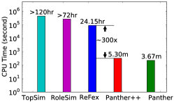
(b) Efficiency Performance

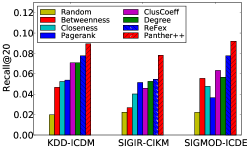
(c) Application: Identity Resolution

Figure 1: Example of top-$k$ similarity search across networks and performance comparison. (a) Top-$k$ similarity search across two disconnected networks; (b) Efficiency comparison of Panther and several comparison methods on a Tencent subnetwork of 443,070 vertices and 5,000,000 edges; and (c) Accuracy performance when applying Panther++ to identity resolution [11], an important application in social network. Please refer to § 4 for definitions of all the comparison methods in (b) and (c).

We propose a sampling-based method, referred to as Panther, that provably and quickly estimates the similarity between vertices. The algorithm is based on a novel idea of random path. Specifically, given a network, we perform $R$ random walks, each starting from a randomly picked vertex and walking $T$ steps. The idea behind this is that two vertices have a high similarity if they frequently appear on the same paths. We provide theoretical proofs for the error-bound and confidence of the proposed algorithm. Theoretically, we obtain that the sample size, $R=\frac{c}{\varepsilon^{2}}(\log_{2}\binom{T}{2}+1+\ln\frac{1}{\delta})$, only depends on the path length $T$ of each random walk, for a given error-bound $\varepsilon$ and confidence level $1-\delta$. To capture the information of structural patterns, we extend the proposed algorithm by augmenting each vertex with a vector of structure-based features. The resultant algorithm is referred to as Panther++. Panther++ is not only able to estimate similarity between vertices in a connected network, but also capable of estimating similarity between vertices from disconnected networks. Figure 1(a) shows an example of top-$k$ similarity search across two disconnected networks, where $v_{4}$, $v_{6}$ and $v_{5}$ are top-3 similar vertices to $v_{0}$.

We evaluate the efficiency of the methods on a microblogging network from Tencent. Figure 1(b) shows the efficiency comparison of Panther, Panther++, and several other methods. Clearly, our methods are much faster than the comparison methods.

Panther++ achieves a 300$\times$ speed-up over the fastest comparison method on a Tencent subnetwork of 443,070 vertices and 5,000,000 edges. Our methods are also scalable. Panther is able to return top-$k$ similar vertices for all vertices in a network with 51,640,620 vertices and 1,000,000,000 edges. On average, it only need 0.0001 second to perform top-$k$ search for each vertex.

We also evaluate the estimation capability of Panther++. Specifically, we use identity resolution and top-$k$ structural hole spanner finding, two important applications in social networks, to evaluate the accuracy of the estimated similarities. Figure 1(c) shows the accuracy performance of Panther++ and several alternative methods for identity resolution. Panther++ achieves clearly better performance than several alternative methods. All codes and datasets used in this paper are publicly available.

Organization Section 2 formulates the problem. In Section 3, we detail the proposed methods for top-$k$ similarity search, and provide theoretical analysis. Section 4 presents experimental results to validate the efficiency and effectiveness of our methods. Section 5 reviews the related work. Finally, Section 6 concludes the paper.

2 Problem Formulation

We first provide necessary definitions and then formally formulate the problem.

Definition 1.

Undirected Weighted Network. Let $G=(V,E,W)$ denotes a network, where $V$ is a set of $|V|$ vertices and $E\subset V\times V$ is a set of $|E|$ edges between vertices. We use $v_{i}\in V$ to represent a vertex and $e_{ij}\in E$ to represent an edge between vertices $v_{i}$ and $v_{j}$. Let $W$ be a weight matrix, with each element $w_{ij}\in W$ representing the weight associated with edge $e_{ij}$.

We use $\mathcal{N}(v_{i})$ to indicate the set of neighboring vertices of vertex $v_{i}$. We leave the study of directed networks to future work. Our purpose here is to estimate similarity between two vertices, e.g., $v_{i}$ and $v_{j}$. We focus on finding top-$k$ similar vertices. Precisely, the problem can be defined as, given a network $G=(V,E,W)$ and a query vertex $v\in V$, how to find a set $X_{v,k}$ of $k$ vertices that have the highest similarities to vertex $v$, where $k$ is a positive integer.

A straightforward method to address the top-$k$ similarity search problem is to first calculate the similarity $s(v_{i},v_{j})$ between vertices $v_{i}$ and $v_{j}$ using metrics such as the Jaccard index and SimRank, and then select a set $X_{v,k}$ of $k$ vertices that have the highest similarities to each vertex $v$. However it is in general difficult to scale up to large networks. One important idea is to obtain an approximate set $X^{*}_{v,k}$ for each vertex. From the accuracy perspective, we aim to minimize the difference between $X^{*}_{v,k}$ and $X_{v,k}$. Formally, we can define the problem studied in this work as follows.

Problem 1.

Top-$k$ similarity search. Given an undirected weighted network $G=(V,E,W)$, a similarity metric $s(.)$, and a positive integer $k$, any vertex $v\in V$, how to quickly and approximately retrieve the top-$k$ similar vertices of $v$? How to guarantee that the difference between the two sets $X^{*}_{v,k}$ and $X_{v,k}$ is less than a threshold $\varepsilon\in(0,1)$, i.e.,

$$\text{Diff}(X^{*}_{v,k},X_{v,k})\leq\varepsilon$$

with a probability of at least $1-\delta$.

The difference between $X^{*}_{v,k}$ and $X_{v,k}$ can be also viewed as the error-bound of the approximation. In the following section, we will propose a sampling-based method to approximate the top-$k$ vertex similarity. We will explain in details how the method can guarantee the error-bound and how it is able to efficiently achieve the goal.

3 Panther: Fast Top-k Similarity Search Using Path Sampling

We begin with considering some baseline solutions and then propose our path sampling approach. A simple approach to the problem is to consider the number of common neighbors of $v_{i}$ and $v_{j}$. If we use the Jaccard index [17], the similarity can be defined as

$$S_{JA}(v_{i},v_{j})=\frac{|\mathcal{N}(v_{i})\cap\mathcal{N}(v_{j})|}{|\mathcal{N}(v_{i})\cup\mathcal{N}(v_{j})|}.$$

This method only considers local information and does not allow vertices to be similar if they do not share neighbors.

To leverage the structural information, one can consider algorithms like SimRank [18]. SimRank estimates vertex similarity by iteratively propagating vertex similarity to neighbors until convergence (no vertex similarity changes), i.e.,

$$S_{SR}(v_{i},v_{j})=\frac{C}{|\mathcal{N}(v_{i})||\mathcal{N}(v_{j})|}\sum_{v_{l}\in\mathcal{N}(v_{i})}\sum_{v_{m}\in\mathcal{N}(v_{j})}s(v_{l},v_{m}),$$

where $C$ is a constant between 0 and 1.

SimRank similarity depends on the whole network and allows vertices to be similar without sharing neighbors. The problem with SimRank is its high computational complexity: $O(I|V|^{2}\bar{d}^{2})$, which makes it infeasible to scale up to large networks. Though quite a few studies have been conducted recently [12, 23], the problem is still largely unsolved.

We propose a sampling-based method to estimate the top-$k$ similar vertices. In statistics, sampling is a widely used technique to estimate a target distribution [36]. Unlike traditional sampling methods, we propose a random path sampling method, named Panther. Given a network $G=(V,E,W)$, Panther randomly generates $R$ paths with length $T$. Then the similarity estimation between two vertices is cast as estimating how likely it is that two vertices appear on a same path. Theoretically we prove that given an error-bound, $\varepsilon$, and a confidence level, $1-\delta$, the sample size $R$ is independent of the network size. Experimentally, we demonstrate that the error-bound is dependent on the number of edges of the network.

3.1 Random Path Sampling

The basic idea of the method is that two vertices are similar if they frequently appear on the same paths. The principle is similar to that in Katz [20].

Path Similarity. To begin with, we introduce how to estimate vertex similarity based on $T$-paths. A $T$-path is defined as a sequence of vertices $p=(v_{1},\cdots,v_{T+1})$, which consists of $T+1$ vertices and $T$ edges. Let $\Pi$ denotes all the $T$-paths in $G$. Let $w(p)$ be the weight of a path $p$. The weight can be defined in different ways. Given this, the path similarity between $v_{i}$ and $v_{j}$ is defined as:

$$S_{RP}(v_{i},v_{j})=\frac{\sum_{p\in P_{v_{i},v_{j}}}w(p)}{\sum_{p\in\Pi}w(p)},$$ (1)

where $P_{v_{i},v_{j}}$ is a subset of $\Pi$ that contain both $v_{i}$ and $v_{j}$.

Estimating Path Similarity with Random Sampling. To calculate the denominator in Eq (1), we need to enumerate all $T$-paths in $G$. However, the time complexity is exponentially proportional to the path length $T$, and thus is inefficient when $T$ increases. Therefore, we propose a sampling-based method to estimate the path similarity. The key idea is that we randomly sample $R$ paths from the network and recalculate Eq (1) based on the sampled paths.

$$S_{RP}(v_{i},v_{j})=\frac{\sum_{p\in P_{v_{i},v_{j}}}w(p)}{\sum_{p\in P}w(p)},$$ (2)

where $P$ is the set of sampled paths.

To generate a path, we randomly select a vertex in $G$ as the starting point, and then conduct random walks of $T$ steps from $v$ using $t_{ij}$ as the transition probability from vertex $v_{i}$ to $v_{j}$.

$$t_{ij}=\frac{w_{ij}}{\sum_{v_{k}\in\mathcal{N}(v_{i})}w_{ik}},$$ (3)

where $w_{ij}$ is the weight between $v_{i}$ and $v_{j}$. In a unweighted network, the transition probability can be simplified as $1/|\mathcal{N}(v_{i})|$.

Based on the random walk theory [7], we define $w(p)$ as

$$w(p)=\prod_{i=1,j=i+1}^{T}t_{ij}.$$

The path weight also represents the probability that a path $p$ is sampled from $\Pi$; thus, $w(p)$ in Eq. (2) is absorbed, and we can rewrite the equation as follows:

$$S_{RP}(v_{i},v_{j})=\frac{|{P}_{v_{i},v_{j}}|}{R}.$$ (4)

Algorithm 3 summarizes the process for generating the $R$ random paths. To calculate Eq. (4), the time complexity is $O(RT)$, because it has to enumerate all $R$ paths. To improve the efficiency, we build an inverted index of vertex-to-path [2]. Using the index, we can retrieve all paths that contain a specific vertex $v$ with a complexity of $O(1)$. Then Eq. (4) can be calculated with a complexity of $O(\bar{R}T)$, where $\bar{R}$ is the average number of paths that contain a vertex and $\bar{R}$ is proportional to the average degree $\bar{d}$. Figure 2 illustrates the process of random path sampling. Details of the algorithm are presented in Algorithm 1.

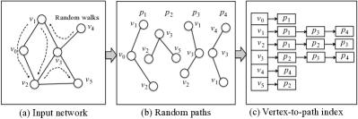
Figure 2: Illustration of random path sampling.

3.2 Theoretical Analysis

We give theoretical analysis for the random path sampling algorithm. In general, the path similarity can be viewed as a probability measure defined over all paths $\Pi$. Thus we can adopt the results from Vapnik-Chernovenkis (VC) learning theory [36] to analyze the proposed sampling-based algorithm. To begin with, we will introduce some basic definitions and fundamental results from Vapnik-Chernovenkis theory, and then demonstrate how to utilize these concepts and results to analyze our method.

Preliminaries. Let $(\mathcal{D},\mathcal{R})$ be a range space, where $\mathcal{D}$ denotes a domain, and $\mathcal{R}$ is a range set on $\mathcal{D}$. For any set $B\subseteq\mathcal{D}$, $P_{\mathcal{R}}(B)=\{B\cap A:A\in\mathcal{R}\}$ is the projection of $\mathcal{R}$ on $B$. If $P_{\mathcal{R}}(B)=2^{B}$, where $2^{B}$ is the powerset of $B$, we say that the set $B$ is shattered by $\mathcal{R}$. The following definitions and theorem derive from [29].

Definition 2.

The Vapnik-Chervonenkis (VC) dimension of $\mathcal{R}$, denoted as $VC(\mathcal{R})$, is the maximum cardinality of a subset of $\mathcal{D}$ that can be shattered by $\mathcal{R}$.

Let $S=\{x_{1},\cdots,x_{n}\}$ be a set of i.i.d. random variables sampled according to a distribution $\phi$ over the domain $\mathcal{D}$. For a set $A\subseteq\mathcal{D}$, let $\phi(A)$ be the probability that an element sampled from $\phi$ belongs to $A$, and let the empirical estimation of $\phi(A)$ on $S$ be

$$\phi_{S}(A)=\frac{1}{n}\sum_{i=1}^{n}\mathds{1}_{A}(x_{i}),$$

where $\mathds{1}_{A}$ is the indicator function with the value of $\mathds{1}_{A}(x)$ equals 1 if $X\in A$, and 0 otherwise.

The question of interest is that how well we can estimate $\phi(A)$ using its unbiased estimator, the empirical estimation $\phi_{S}(A)$. We first give the goodness of approximation in the following definition.

Definition 3.

Let $\mathcal{R}$ be a range set on $\mathcal{D}$, and $\phi$ be a probability distribution defined on $\mathcal{D}$. For $\varepsilon\in(0,1)$, an $\varepsilon$-approximation to $(\mathcal{R},\phi)$ is a set $S$ of elements in $\mathcal{D}$ such that

$$sup_{A\in\mathcal{R}}|\phi(A)-\phi_{S}(A)|\leq\varepsilon.$$

One important result of VC theory is that if we can bound the $VC$-dimension of $\mathcal{R}$, it is possible to build an $\varepsilon$-approximation by randomly sampling points from the domain according to the distribution $\phi$. This is summarized in the following theorem.

Theorem 1.

Let $\mathcal{R}$ be a range set on a domain $\mathcal{D}$, with $VC(\mathcal{R})\leq d$, and let $\phi$ be a distribution on $\mathcal{D}$. Given $\varepsilon,\delta\in(0,1)$ , let $S$ be a set of $|S|$ points sampled from $\mathcal{D}$ according to $\phi$, with

$$|S|=\frac{c}{\varepsilon^{2}}(d+\ln\frac{1}{\delta}),$$

where $c$ is a universal positive constant. Then $S$ is a $\varepsilon$-approximation to $(\mathcal{R},\phi)$ with probability of at least $1-\delta$.

Range Set of Path. In our setting, we set the domain to be $\Pi$—the set of all paths with length $T$ in the graph $G$. Accordingly, we define the range set $\mathcal{R}_{G}$ on domain $\Pi$ to be

$$\mathcal{R}_{G}=\{P_{v_{i},v_{j}}:v_{i},v_{j}\in V\}.$$

It is a valid range set, since it is the collection of subsets $P_{v_{i},v_{j}}$ of domain $\Pi$. We first show an upper bound of the VC dimension of $\mathcal{R}_{G}$ in Lemma 1. The proof is inspired by  [29].

Lemma 1.

$VC(\mathcal{R}_{G})\leq\log_{2}\binom{T}{2}+1$

Proof.

We prove the lemma by contradiction. Assume $VC(\mathcal{R}_{G})=l$ and $l>\log_{2}\binom{T}{2}+1$. By the definition of VC-dimension, there is a set $Q\subseteq\Pi$ of size $l$ that can be shattered by $\mathcal{R}_{G}$. That is, we have the following statement:

$$\forall S_{i}\subseteq Q\text{ , }\exists P_{i}\in\mathcal{R}_{G}\text{, ~{}~{}~{}~{}s.t. }P_{i}\cap Q=S_{i},$$

where $P_{i}$ is the $i$-th range. Since each subset $S_{i}\in Q$ is different from the other subsets, the corresponding range $P_{i}$ that making $P_{i}\cap Q=S_{i}$ is also different from the other ranges. Moreover, the set $Q$ is shattered by $\mathcal{R}_{G}$ if and only if $\{P_{i}\cap Q:P_{i}\in\mathcal{R}\}=2^{Q}$. Thus $\forall p\in Q$, there are $2^{l-1}$ non-empty distinct subsets $S_{1},\cdots,S_{2^{l-1}}$ of $Q$ containing the path $p$. So there are also $2^{l-1}$ distinct ranges in $\mathcal{R}_{G}$ that contain the path $p$, i.e.

$$|\{P_{i}|p\in P_{i}\text{ and }P_{i}\in\mathcal{R}_{G}\}|=2^{l-1}.$$

In addition, according to the definition of range set, $\mathcal{R}_{G}=\{P_{v_{i},v_{j}}:v_{i},v_{j}\in V\}$, we know that a path belongs only to the ranges corresponding to any pair of vertices in path $p$, i.e., to the pairwise combinations of the vertices in $p$. This means the number of ranges in $\mathcal{R}_{G}$ that $p$ belongs to is equal to the combinatorial number $\binom{T}{2}$, i.e.,

$$|\{P_{i}|p\in P_{i}\text{ and }P_{i}\in\mathcal{R}_{G}\}|=\binom{T}{2}.$$

On the other hand, from our preliminary assumption, we have $l>\log_{2}\binom{T}{2}+1$, which is equivalent to $\binom{T}{2}<2^{l-1}$. Thus,

$$|\{P_{i}|p\in P_{i}\text{ and }P_{i}\in\mathcal{R}_{G}\}|=\binom{T}{2}<2^{l-1}.$$

Hence, we reach a contradiction: it is impossible to have $2^{l-1}$ distinct ranges $P_{i}\in\mathcal{R}_{G}$ containing $p$. Since there is a one-to-one correspondence between $S_{i}$ and $P_{i}$, we get that it is also impossible to have $2^{l-1}$ distinct subset $S_{i}\in Q$ containing $p$. Therefore, we prove that $Q$ cannot be shattered by $\mathcal{R}_{G}$ and $VC(\mathcal{R}_{G})\leq\log_{2}\binom{T}{2}+1.$ ∎

Sample Size Guarantee. We now provide theoretical guarantee for the number of sampled paths. How many random paths do we need to achieve an error-bound $\varepsilon$ with probability $1-\delta$? We define a probability distribution on the domain $\Pi$. $\forall p\in\Pi$, we define

$$\phi(p)=\text{prob}(p)=\frac{w(p)}{\sum_{p\in\Pi}w(p)}.$$

We can see that the definition of $S_{RP}(v_{i},v_{j})$ in Eq.(1) is equivalent to $\phi(P_{v_{i},v_{j}})$. This observation enables us to use a sampling-based method (empirical average) to estimate the original path similarity (true probability measure).

Plugging the result of Lemma (1) into Theorem (1), we obtain:

$$R=\frac{c}{\varepsilon^{2}}(\log_{2}\binom{T}{2}+1+\ln\frac{1}{\delta}).$$

That is, with at least $R$ random paths, we can estimate the path similarity between any two vertices with the desired error-bound and confidence level. The above equation also implies that the sample size $R$ only depends on the path length $T$, given an error-bound $\varepsilon$, and a confidence level $1-\delta$.

Input: A network $G=(V,E,W)$, path length $T$, parameters $\varepsilon$, $c$, $\delta$, a vertex $v$, and $k$.

Output: top-$k$ similar vertices with regard to $v$.

Calculate sample size $R=\frac{c}{\varepsilon^{2}}(\log_{2}\binom{T}{2}+1+\ln\frac{1}{\delta})$ ;

GenerateRandomPath($G$, $R$);

foreach $p_{n}\in P_{v}$ do  foreach Unique $v_{j}\in p_{n}$ do  $S_{RP}(v,v_{j})+=\frac{1}{R}$ ;

    Retrieve top-$k$ similar vertices according to $S_{RP}(v,v_{j})$;

Algorithm 1 Panther

5

5

5

5

5

Input: A network $G=(V,E,W)$, path length $T$, parameters $\varepsilon$, $c$, $\delta$, vector dimension $D$, a vertex $v$, and $k$.

Output: top-$k$ similar vertices with regard to $v$.

Calculate sample size $R=\frac{c}{\varepsilon^{2}}(\log_{2}\binom{T}{2}+1+\ln\frac{1}{\delta})$ ;

GenerateRandomPath($G$, $R$);

foreach $v_{i}\in V$ do  foreach $p_{n}\in P_{v_{i}}$ do  foreach Unique $v_{j}\in p_{n}$ do  $S_{RP}(v_{i},v_{j})+=\frac{1}{R}$ ;

    Construct a vector $\theta(v_{i})$ by taking the largest $D$ values from $\{S_{RP}(v_{i},v_{j}):v_{j}\in p_{n}\text{ and }p_{n}\in P_{v_{i}}\}$;

  Build a kd-tree index based on the Euclidean distance between any vectors $\theta(v_{i})$ and $\theta(v_{j})$ ;

Query the top-$k$ similar vertices from the index for $v$;

Algorithm 2 Panther++

7

7

7

7

7

7

7

Input: A network $G=(V,E,W)$ and sample size $R$.

Output: Paths $\{p_{r}\}_{r=1}^{R}$ and vertex-to-path index $\{P_{v_{i}}\}_{i=1}^{N}$.

Calculate transition probabilities between every pair of vertices according to Eq. (3) ;

Initialize $r=1$;

repeat  Sample current vertex $v=v_{i}$ uniformly at random ;

Add $v$ into $p_{r}$ and add $p_{r}$ into the path set of $v$, i.e., $P_{v}$ ;

repeat  Randomly sample a neighbor $v_{j}$ according to transition probabilities from $v$ to its neighbors;

Set current vertex $v=v_{j}$;

Add $v$ into $p_{r}$ and add $p_{r}$ into $P_{v}$ ;

until $|p_{r}|<T+1$;

$r+=1$;

until $r<R$;

Algorithm 3 GenerateRandomPath

12

12

12

12

12

12

12

12

12

12

12

12

3.3 Panther++

One limitation of Panther is that the similarities obtained by the algorithm have a bias to close neighbors, though in principle it considers the structural information. We therefore present an extension of the Panther algorithm. The idea is to augment each vertex with a feature vector. To construct the feature vector, we follow the intuition that the probability of a vertex linking to all other vertices is similar if their topology structures are similar [15]. We select the top-$D$ similarities calculated by Panther to represent the probability distribution. Specifically, for vertex $v_{i}$ in the network, we first calculate the similarity between $v_{i}$ and all the other vertices using Panther. Then we construct a feature vector for $v_{i}$ by taking the largest $D$ similarity scores as feature values, i.e.,

$$\theta(v_{i})=(S_{RP}(v_{i},v_{(1)}),S_{RP}(v_{i},v_{(2)}),\ldots,S_{RP}(v_{i},v_{(D)})),$$

where $S_{RP}(v_{i},v_{(d)})$ denotes the $d$-th largest path similarity between $v_{i}$ and another vertex $v_{(d)}$.

Finally, the similarity between $v_{i}$ and $v_{j}$ is re-calculated as the reciprocal Euclidean distance between their feature vectors:

$$S_{RP^{++}}(v_{i},v_{j})=\frac{1}{\lVert\theta(v_{i})-\theta(v_{j})\rVert}.$$

The idea of using vertex features to estimate vertex similarity was also used for graph mining [14].

Index of Feature Vectors Again, we use the indexing techniques to improve the algorithm efficiency. We build a memory based kd-tree [37] index for feature vectors of all vertices. Then given a vertex, we can retrieve top-$k$ vertices in the kd-tree with the least Euclidean distance to the query vertex efficiently. At a high level, a kd-tree is a generalization of a binary search tree that stores points in $D$-dimensional space. In level $h$ of a kd-tree, given a node $v$, the $h\%D$-th element in the vector of each node in its left subtree is less than the $h\%D$-th element in the vector of $v$, while the $h\%D$-th element of every node in the right subtree is no less than the $h\%D$-th element of $v$. Figure 3 shows the data structure of the index built in Panther++. Based on the index, we can query whether a given point is stored in the index very fast. Specifically, given a vertex $v$, if the root node is $v$, return the root node. If the first element of $v$ is strictly less than the first element of the root node, look for $v$ in the left subtree, then compare it to the second element of $v$. Otherwise, check the right subtree. It is worth noting that we can easily replace kd-tree with any other index methods, such as r-tree. The algorithms for calculating feature vectors of all vertices and the similarity between vertices are shown in Algorithm 2.

Figure 3: Data structure of the index built in Panther++.

Implementation Notes. In our experiments, we empirically set the parameters as follows: $c=0.5$, $\delta=0.1$, $T=5$, $D=50$ and $\varepsilon=\sqrt{1/|E|}$. The optimal values of $T$, $D$ and $\varepsilon$ are discussed in section 4. We build the kd-tree using the toolkit ANN.

Table 1: Time and space complexity for calculating top-$k$ similar vertices for all vertices in a network. $I$— number of iterations, $\bar{d}$—average degree, $f$—feature number, $D$ — vector dimension, and $T$ — path length.

Method	Time Complexity	Space Complexity
SimRank [18]	$O(I|V|^{2}\bar{d}^{2})$	$O(|V|^{2})$
TopSim [23]	$O(|V|T\bar{d}^{T})$	$O(|V|+|E|)$
RWR [28]	$O(I|V|^{2}\bar{d})$	$O(|V|^{2})$
RoleSim [19]	$O(I|V|^{2}\bar{d}^{2})$	$O(|V|^{2})$
ReFex [14]	$O(|V|+I(f|E|+|V|f^{2}))$	$O(|V|+|E|f)$
Panther	$O(RTc+|V|\bar{d}T)$	$O(RT+|V|\bar{d})$
Panther++	$O(RTc+|V|\bar{d}T+|V|c)$	$O(RT+|V|\bar{d}+|V|D)$

3.4 Complexity Analysis

In general, existing methods result in high complexities. For example, the time complexity of SimRank [18], TopSim [23], Random walk with restart (RWR) [28], RoleSim [19], and ReFex [14] is $O(I|V|^{2}\bar{d}^{2})$, $O(|V|T\bar{d}^{T})$, $O(I|V|^{2}\bar{d})$, $O(I|V|^{2}\bar{d}^{2})$, and $O(|V|+I(f|E|+|V|f^{2}))$, respectively. Table 1 summarizes the time and space complexities of the different methods. For Panther, its time complexity includes two parts:

• Random path sampling: The time complexity of generating random paths is $O(RT\log\bar{d})$, where $\log\bar{d}$ is very small and can be simplified as a small constant $c$. Hence, the time complexity is $O(RTc)$.

• Top-$k$ similarity search: The time complexity of calculating top-$k$ similar vertices for all vertices is $O(|V|\bar{R}T+|V|\bar{M})$. The first part $O(|V|\bar{R}T)$ is the time complexity of calculating Eq. (4) for all pairs of vertices, where $\bar{R}$ is the average number of paths that contain a vertex and is proportional to the average degree $\bar{d}$. The second part $O(|V|\bar{M})$ is the time complexity of searching top-$k$ similar vertices based on a heap structure, where $\bar{M}$ represents the average number of co-occurred vertices with a vertex and is proportional to $\bar{d}$. Hence, the time complexity is $O(|V|\bar{d}T)$.

The space complexity for storing paths and vertex-to-path index is $O(RT)$ and $O(|V|\bar{d})$, respectively.

Panther++ requires additional computation to build the kd-tree. The time complexity of building a kd-tree is $O(|V|\log|V|)$ and querying top-$k$ similar vertices for any vertex is $O(|V|\log|V|)$, where $\log|V|$ is small and can be viewed as a small constant $c$. Additional space (with a complexity of $O(|V|D)$) is required to store $|V|$ vectors with $D$-dimension.

4 Experiments

4.1 Experimental Setup

In this section, we conduct various experiments to evaluate the proposed methods for top-$k$ similarity search.

Datasets. We evaluate the proposed method on four different networks: Tencent, Twitter, Mobile, and co-author.

Tencent [38]: The dataset is from Tencent Weibo, a popular Twitter-like microblogging service in China, and consists of over 355,591,065 users and 5,958,853,072 “following” relationships. The weight associated with each edge is set as 1.0 uniformly. This is the largest network in our experiments. We mainly use it to evaluate the efficiency performance of our methods.

Twitter [16]: The dataset was crawled in the following way. We first selected the most popular user on Twitter, i.e., “Lady Gaga”, and randomly selected 10,000 of her followers. We then collected all followers of these users. In the end, we obtained 113,044 users and 468,238 “following” relationships in total. The weight associated with each edge is also set as 1.0 uniformly. We use this dataset to evaluate the accuracy of Panther and Panther++.

Mobile [6]: The dataset is from a mobile communication company, and consists of millions of call records. Each call record contains information about the sender, the receiver, the starting time, and the ending time. We build a network using call records within two weeks by treating each user as a vertex, and communication between users as an edge. The resultant network consists of 194,526 vertices and 206,934 edges. The weight associated with each edge is defined as the number of calls. We also use this dataset to evaluate the accuracy of the proposed methods.

Co-author [34]: The dataset is from AMiner.org, and contains 2,092,356 papers. From the original citation data, we extracted a weighted co-author graph from each of the following conferences from 2005 to 2013: KDD, ICDM, SIGIR, CIKM, SIGMOD, ICDE, and ICML. The weight associated with each edge is the number of papers collaborated on by the two connected authors. We also use the dataset to evaluate the accuracy of the proposed methods.

Evaluation Aspects. To quantitatively evaluate the proposed methods, we consider the following performance measurements:

Efficiency Performance: We apply our methods to the Tencent network to evaluate the computational time.

Accuracy Performance: We apply the proposed methods to recognize identical authors on different co-author networks. We also apply our methods to the Coauthor, Twitter and Mobile networks to evaluate how they estimate the top-$k$ similarity search results.

Parameter Sensitivity Analysis: We analyze the sensitivity of different parameters in our methods: path length $T$, vector dimension $D$, and error-bound $\varepsilon$.

Finally, we also use several case studies as anecdotal evidence to further demonstrate the effectiveness of the proposed method. All codes are implemented in C++ and compiled using GCC 4.8.2 with -O3 flag. The experiments were conducted on a Ubuntu server with four Intel Xeon(R) CPU E5-4650 (2.70GHz) and 1T RAM.

Comparison methods. We compare with the following methods:

RWR [28]: Starts from $v_{i}$, iteratively walks to its neighbors with the probability proportional to their edge weights. At each step, it also has some probability to walk back to $v_{i}$ (set as 0.1). The similarity between $v_{i}$ and $v_{j}$ is defined as the steady-state probability that $v_{i}$ will finally reach at $v_{j}$. We calculate RWR scores between all pairs and then search the top-$k$ similar vertices for each vertex.

TopSim [23]: Extends SimRank [18] on one graph $G$ to finding top-$k$ authoritative vertices on the product graph $G\times G$ efficiently.

RoleSim [19]: Refines SimRank [18] by changing the average similarity of all neighbor pairs to all matched neighbor pairs. We calculate RoleSim scores between all pairs and then search the top-$k$ similar vertices for each vertex.

ReFeX [14]: Defines local, egonet, and recursive features to capture the structural characteristic. Local feature is the vertex degree. Egonet features include the number of within-egonet edges and the number of out-egonet edges. For weighted networks, they contain weighted versions of each feature. Recursive features are defined as the mean and sum value of each local or egonet feature among all neighbors of a vertex. In our experiments, we only extract recursive features once and construct a vector for each vertex by a total of 18 features. For fair comparison, to search top-$k$ similar vertices, we also build the same kd-tree as that in our method.

The codes of TopSim, RoleSim, and ReFex are provided by the authors of the original papers. We tried to use the fast versions of TopSim and RoleSim mentioned in their paper.

Table 2: Efficiency performance (CPU time) of comparison methods on different sizes of the Tencent sub-networks. The time includes all computational cost for processing and top-$k$ similarity search for all vertices. The time before “+” denotes the time used for processing and the time after “+” denotes that used for top-$k$ similarity search. “—” indicates that the corresponding algorithm cannot finish the computation within a reasonable time.

Sub-network	|V|	|E|	RWR	TopSim	RoleSim	ReFeX	Panther	Panther++
Tencent1	6,523	10,000	+7.79hr	+28.58m	+37.26s	3.85s+0.07s	0.07s+0.26s	0.99s+0.21s
Tencent2	25,844	50,000	+>150hr	+11.20hr	+12.98m	26.09s+0.40s	0.28s+1.53s	2.45s+4.21s
Tencent3	48,837	100,000	—	+30.94hr	+1.06hr	2.02m+0.57s	0.58s+ 3.48s	5.30s+5.96s
Tencent4	169,209	500,000	—	+>120hr	+>72 hr	17.18m+2.51s	8.19s+16.08s	27.94s+24.17s
Tencent5	230,103	1,000,000	—	—	—	31.50m+3.29s	15.31s+30.63s	49.83s+22.86s
Tencent6	443,070	5,000,000	—	—	—	24.15hr+8.55s	50.91s+2.82m	4.01m+1.29m
Tencent7	702,049	10,000,000	—	—	—	>48hr	2.21m+6.24m	8.60m+6.58m
Tencent8	2,767,344	50,000,000	—	—	—	—	15.78m+1.36hr	1.60hr+2.17hr
Tencent9	5,355,507	100,000,000	—	—	—	—	44.09m +4.50hr	5.61hr +6.47hr
Tencent10	26,033,969	500,000,000	—	—	—	—	4.82hr +25.01hr	32.90hr +47.34hr
Tencent11	51,640,620	1,000,000,000	—	—	—	—	13.32hr +80.38hr	98.15hr +120.01hr

4.2 Efficiency and Scalability Performance

In this subsection, we first fix $k=5$, and evaluate the efficiency and scalability performance of different comparison methods using the Tencent dataset. We evaluate the performance by randomly extracting different (large and small) versions of the Tencent networks. For TopSim and RoleSim, we only show the computational time for similarity search. For ReFex, Panther, and Panther++, we also show the computational time used for preprocessing.

Table 2 lists statistics of the different Tencent sub-networks and the efficiency performance of the comparison methods. Clearly, our methods (both Panther and Panther++) are much faster than the comparison methods. For example, on the Tencent6 sub-network, which consists of 443,070 vertices and 5,000,000 edges, Panther achieves a $390\times$ speed-up , compared to the fastest (ReFeX) of all the comparative methods.

Figure 4(a) shows the speed-up of Panther++ compared to ReFeX on different scales of sub-networks. The speed-up is moderate when the size of the network is small ($|E|\leq 1,000,000$); when continuing to increase the size of the network, the obtained speed-up is even superlinear. We conducted a result comparison between ReFeX and Panther++. The results of Panther++ are very similar to those of ReFex, though they decrease slightly when the size of the network is small. Figure 4(b) shows the efficiency performance of Panther and Panther++ by varying the values of $k$ from 5 to 100. We can see that the time costs of Panther and Panther++ are not very sensitive to $k$. The growth of time cost is slow when $k$ gets larger. This is because $k$ is only related to the time complexity of top-$k$ similarity search based on a heap structure. When $k$ gets larger, the time complexity approximates to $O(\bar{M}\log\bar{M})$ from $O(\bar{M})$, where $\bar{M}$ is the average number of co-occurred vertices on the same paths. We can also see that the time cost is not very stable when $k$ gets larger, because the paths are randomly generated, which results in different values of $\bar{M}$ each time.

From Table 2, we can also see that RWR, TopSim and RoleSim cannot complete top-$k$ similarity search for all vertices within a reasonable time when the number of edges increases to 500,000. ReFeX can deal with larger networks, but also fails when the edge number increases to 10,000,000. Our methods can scale up to handle very large networks with more than 10,000,000 edges. On average, Panther only needs 0.0001 second to perform top-$k$ similarity search for each vertex in a large network.

(a) Speed-up

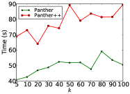
(b) Effect of $k$

Figure 4: (a) Performance ratio is calculated by $\frac{\text{Score(ReFex)}}{\text{Score(Panther++)}}$, where score is evaluated by the application of structural hole spanner finding (see § 4.3 for details.); Speed-up is calculated by $\frac{\text{Time(ReFex)}}{\text{Time(Panther++)}}$; (b) Effect of $k$ on the efficiency performance of Panther and Panther++.

4.3 Accuracy Performance with Applications

Identity Resolution. It is difficult to find a ground truth to evaluate the accuracy for similarity search. To quantitatively evaluate the accuracy of the proposed methods and compare with the other methods, we consider an application of identity resolution on the co-author network. The idea is that we first use the authorship at different conferences to generate multiple co-author networks. An author may have a corresponding vertex in each of the generated networks. We assume that the same authors in different networks of the same domain are similar to each other. We anonymize author names in all the networks. Thus given any two co-author networks, for example KDD-ICDM, we perform a top-$k$ search to find similar vertices from ICDM for each vertex in KDD by different methods. If the returned $k$ similar vertices from ICDM by a method consists of the corresponding author of the query vertex from KDD, we say that the method hits a correct instance. A similar idea was also employed to evaluate similarity search in [11]. Please note that the search is performed across two disconnected networks. Thus, RWR, TopSim and RoleSim cannot be directly used for solving the task. ReFex calculates a vector for each vertex, and can be used here. Additionally, we also compare with several other methods including Degree, Clustering Coefficient, Closeness, Betweenness and Pagerank. In our methods, Panther is not applicable to this situation. We only evaluate Panther++ here. Additionally, we also show the performance of random guess.

Figure 5 presents the performance of Panther++ on the task of identity resolution across co-author networks. We see that Panther++ performs the best on all three datasets. ReFex performs comparably well; however, it is not very stable. In the SIGMOD-ICDE case, it performs the same as Panther++, while in the KDD-ICDM and SIGIR-CIKM cases, it performs worse than Panther++, when $k\leq 60$.

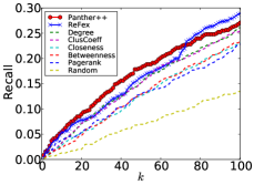
(a) KDD-ICDM

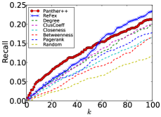
(b) SIGIR-CIKM

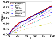
(c) SIGMOD-ICDE

Figure 5: Performance of identity resolution across two networks with different comparison methods.

Approximating Common Neighbors. We evaluate how Panther can approximate the similarity based on common neighbors. The evaluation procedure is described as follows:

1. For each vertex $u$ in the seed set $S$, generate top $k$ vertices $\text{Top}_{A,k}(u)$ that are the most similar to $u$ by the algorithm $A$.

2. For each vertex $v\in\text{Top}_{A,k}(u)$, calculate $g(u,v)$, where $g$ is a coarse similarity measure defined as the ground truth. Define $f_{A,k}=\sum_{u}\sum_{v}g(u,v)$.

3. Similarly, let $f_{R,k}$ denotes the result of a random algorithm.

4. Finally, we define the score for algorithm $A$ as $\text{score}(A,k)=\frac{f_{A,k}-f_{R,k}}{|S|\times k}$, which represents the improvement of algorithm $A$ over a random-based method.

Specifically, we define $g(u,v)$ to be the number of common neighbors between $u$ and $v$ on each dataset.

Figure 6 shows the performance of Panther evaluated on the ground truth of common neighbors in different networks. Some baselines such as RWR and RoleSim are ignored on different datasets, because they cannot complete top-$k$ similarity search for all vertices within a reasonable time. It can be seen that Panther performs better than any other methods on most datasets. Panther++, ReFex and Rolesim perform worst since they are not devised to address the similarity between near vertices. Our method Panther performs as good as TopSim, the top-$k$ version of SimRank, because they both based on the principle that two vertices are considered structuraly equivalent if they have many common neighbors in a network. However, according to our previous analysis, TopSim performs much slower than Panther.

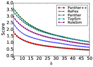
(a) KDD

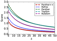
(b) SIGIR

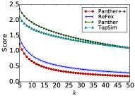
(c) Twitter

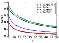
(d) Mobile

Figure 6: Performance of Panther evaluated on the ground truth of common neighbors.

Top-$k$ Structural Hole Spanner Finding. The other application we consider in this work is top-$k$ structural hole spanner finding. The theory of structural holes [5] suggests that, in social networks, individuals would benefit from filling the “holes” between people or groups that are otherwise disconnected. The problem of finding top-$k$ structural hole spanners was proposed in [26], which also shows that 1% of users who span structural holes control 25% of the information diffusion (retweeting) in Twitter.

Structural hole spanners are not necessarily connected, but they share the same structural patterns such as local clustering coefficient and centrality. Thus, the idea here is to feed a few seed users to the proposed Panther++, and use it to find other structural hole spanners. For evaluation, we use network constraint [5] to obtain the structural hole spanners in Twitter and Mobile, and use this as the ground truth. Then we apply different methods—Panther++, ReFex, Panther, and SimRank—to retrieve top-$k$ similar users for each structural hole spanner. If an algorithm can find another structural hole spanner in the top-$k$ returned results, then it makes a correct search. We define $g(u,v)=1$, if both $u$ and $v$ are structural hole spanners, and $g(u,v)=0$ otherwise.

Figure 7 shows the performance of comparison methods for finding structural hole spanners in different networks. Panther++ achieves a consistently better performance than the comparison methods by varying the value of $k$. TopSim, the top-$k$ version of SimRank seems inapplicable to this task. This is reasonable, as the underlying principle of SimRank is to find vertices with more connections to the query vertex.

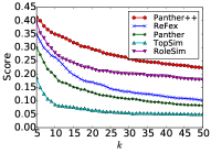
(a) KDD

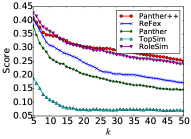
(b) SIGIR

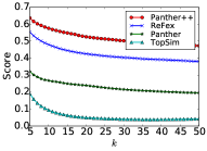
(c) Twitter

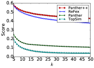
(d) Mobile

Figure 7: Performance of mining structural hole spanners on the Twitter and Mobile networks with different methods.

4.4 Parameter Sensitivity Analysis

We now discuss how different parameters influence the performance of our methods.

Effect of Path Length $T$. Figure 8 shows the accuracy performance of Panther++ for mining structural holes by varying the path length $T$ as 2, 5, 10, 20 , 50 and 100. A too small $T(<5)$ would result in inferior performance. On Twitter, when increasing its value up to 5, it almost becomes stable. On Mobile, the situation is a bit complex, but in general $T=5$ seems to be a good choice.

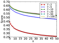
(a) Twitter

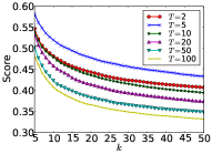
(b) Mobile

Figure 8: Effect of path length $T$ on the accuracy performance of Panther++.

Effect of Vector Dimension $D$. Figure 9 shows the accuracy performance of Panther++ for mining structural hole spanners by varying vector dimension $D$ as 2, 5, 10, 20, 50 and 100. Generally speaking, the performance gets better when $D$ increases and it remains the same after $D$ gets larger than 50. This is reasonable, as Panther estimates the distribution of a vertex linking to the other vertices. Thus, the higher the vector dimension, the better the approximation. Once the dimension exceeds a threshold, the performance gets stable.

Effect of Error Bound $\varepsilon$. Figure 10 shows the accuracy performance of Panther and Panther++ on the Tencent networks with different scales by varying error-bound $\varepsilon$ from 0.06 to 0.0001. We evaluate how Panther can estimate the similarity based on common neighbors. Specifically, we use the same evaluation methods as structural hole spanner finding and define $g(u,v)$ to be the number of common neighbors between $u$ and $v$ on each dataset. We see that when the ratio $\frac{|E|}{(1/\varepsilon)^{2}}$ ranges from 5 to 20, scores of Panther are almost convergent on all the datasets. And when the ratio $\frac{|E|}{(1/\varepsilon)^{2}}$ ranges from 0.2 to 5, the scores of Panther++ are almost convergent on all the datasets. Thus we can reach the conclusion that the value of $(1/\varepsilon)^{2}$ is almost linearly positively correlated with the number of edges in a network. Therefore we can empirically estimate $\varepsilon=\sqrt{1/|E|}$ in our experiments.

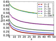
(a) Twitter

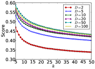
(b) Mobile

Figure 9: Effect of vector dimension $D$ on the accuracy performance of Panther++.

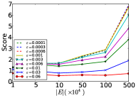
(a) Panther

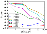
(b) Panther++

Figure 10: Effect of error-bound $\varepsilon$ on the performance of Panther and Panther++ on different sizes of Tencent networks.

4.5 Qualitative Case study

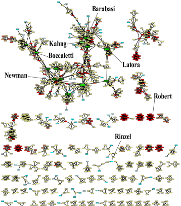
Figure 11: Case study in a scientific co-author network [27]. The authors in similar positions to that of Barabási are denoted in green, similar to that of Robert are in red, and similar to that of Rinzel are in blue. Others are in yellow.

Now we present two case studies to demonstrate the effectiveness of the proposed methods.

“Similar Researchers” Table 3 shows an example of top-5 similar authors to Jiawei Han, Michael I. Jordan, and W. Bruce Croft, found by Panther and Panther++. The two methods present very different results. Those authors found by Panther have closer connections with the query author. While those authors found by Panther++ have a similar “social status” (essentially similar structural patterns) to the query author. For example, Philip S. Yu and Christos Faloutsos are two researchers as famous as Jiawei Han in the data mining field (KDD). Andrew Y. Ng and Bernhard Scholkopft are influential researchers similar to Michael I. Jordan in the machine learning field (ICML).

Table 3: Case study of top-5 similar authors in KDD, ICML and SIGIR networks.

Jiawei Han		Michael I. Jordan		W. Bruce Croft
Panther	Panther++	Panther	Panther++	Panther	Panther++
Chi Wang	Philip S. Yu	Eric p. Xing	Andrew Y. Ng	Michael Bendersky	Leif Azzopardi
Jing Gao	Christos Faloutsos	Percy Liang	Bernhard Scholkopf	Trevor Strohman	Maarten de Rijke
Xifeng Yan	Jeping Ye	Lester W. Mackey	Zoubin Ghahramani	Jangwon Seo	Zheng Chen
YiZhou Sun	Naren Ramakrishnan	Gert R. G. Lanckriet	Michael l. Littman	Donald Metzler	Ryen w. White
Philip S. Yu	Ravi Kumar	Purnamrita Sarkar	Thomas G. Dietterich	Jiwoon Jeon	Chengxiang Zhai

“Who is similar to Barabási?” Albert-László Barabási is a famous Hungarian-American physicist, who proposed the Barabási–Albert (BA) model for generating random scale-free networks using a preferential attachment mechanism. We apply Panther++ to a scientific network [13, 27] to find researchers who have similar structural positions to that of Dr. Barabási. It is interesting that different researchers play different roles in the network. Mark Newman and Vito Latora have similar structural patterns to that of Dr. Barabási. Some other researchers like Robert form a tight-knit group with him. Panther++ successfully recognizes those researchers with similar structural positions.

5 Related Work

Early similarity measures, including bibliographical coupling [21] and co-citation [32] are based on the assumption that two vertices are similar if they have many common neighbors. This category of methods cannot estimate similarity between vertices without common neighbors. Several measures have been proposed to address this problem. For example, Katz [20] counts two vertices as similar if there are more and shorter paths between them. Tsourakakis et al. [35] learn a low-dimension vector for each vertex from the adjacent matrix and calculate similarities between the vectors. Jeh and Widom [18] propose a new algorithm, SimRank. The algorithm follows a basic recursive intuition that two nodes are similar if they are referenced by similar nodes. VertexSim [27] is an extension of SimRank. However, all the SimRank-based methods share a common drawback: their computational complexities are too high. Further studies have been done to reduce the computational complexity of SimRank [12, 22, 23]. Fast-random-walk-based graph similarity, such as in [10, 31], has also been studied recently. Sun et al. [33] measure similarities between vertices based on their inter-paths instantiated from different schemes defined in a heterogeneous information network. The setting is different from ours and the algorithm is not efficient.

Most aforementioned methods cannot handle similarity estimation across different networks. Blondel et al. [3] provide a HITS-based recursive method to measure similarity between vertices across two different graphs. RoleSim [19] can also calculate the similarity between disconnected vertices. Similar to SimRank, the computational complexity of the two methods is very high. Feature-based methods can match vertices with similar structures. For example, Burt [4] counts the 36 kinds of triangles in one’s ego network to represent a vertex’s structural characteristic. In the same way, vertex centrality, closeness centrality, and betweenness centrality [8] of two different vertices can be compared, to produce a structural similarity measure. Aoyama et al. [1] present a fast method to estimate similarity search between objects, instead of vertices in networks. ReFex [14, 13] defines basic features such as degree, the number of within/out-egonet edges, and define the aggregated values of these features over neighbors as recursive features. The computational complexity of ReFex depends on the recursive times. More references about feature-based similarity search in networks can be found in the survey [30].

6 Conclusion

In this paper, we propose a sampling method to quickly estimate top-$k$ similarity search in large networks. The algorithm is based on the idea of random path and an extended method is also presented to enhance the structural similarity when two vertices are completely disconnected. We provide theoretical proofs for the error-bound and confidence of the proposed algorithm. We perform an extensive empirical study and show that our algorithm can obtain top-$k$ similar vertices for any vertex in a network approximately 300$\times$ faster than state-of-the-art methods. We also use identity resolution and structural hole spanner finding, two important applications in social networks, to evaluate the accuracy of the estimated similarities. Our experimental results demonstrate that the proposed algorithm achieves clearly better performance than several alternative methods.

Acknowledgements. The authors thank Pei Lee, Laks V.S. Lakshmanan, Jeffrey Xu Yu; Ruoming Jin, Victor E. Lee, Hui Xiong; Keith Henderson, Brian Gallagher, Lei Li, Leman Akoglu, Tina Eliassi-Rad, Christos Faloutsos for sharing codes of the comparation methods. We thank Tina Eliassi-Rad for sharing datasets.

References

- [1] K. Aoyama, K. Saito, H. Sawada, and N. Ueda. Fast approximate similarity search based on degree-reduced neighborhood graphs. In KDD’11, pages 1055–1063, 2011.
- [2] R. Baeza-Yates, B. Ribeiro-Neto, et al. Modern information retrieval, volume 463. ACM press, 1999.
- [3] V. D. Blondel, A. Gajardo, M. Heymans, P. Senellart, and P. Van Dooren. A measure of similarity between graph vertices: Applications to synonym extraction and web searching. SIAM review, 46(4):647–666, 2004.
- [4] R. S. Burt. Detecting role equivalence. Social Networks, 12(1):83–97, 1990.
- [5] R. S. Burt. Structural holes: The social structure of competition. Harvard university press, 2009.
- [6] Y. Dong, Y. Yang, J. Tang, Y. Yang, and N. V. Chawla. Inferring user demographics and social strategies in mobile social networks. In KDD’14, pages 15–24, 2014.
- [7] W. Feller. An introduction to probability theory and its applications, volume 2. John Wiley & Sons, 2008.
- [8] L. C. Freeman. A set of measures of centrality based on betweenness. Sociometry, pages 35–41, 1977.
- [9] L. C. Freeman. Centrality in social networks conceptual clarification. Social networks, 1(3):215–239, 1979.
- [10] Y. Fujiwara, M. Nakatsuji, H. Shiokawa, T. Mishima, and M. Onizuka. Efficient ad-hoc search for personalized pagerank. In SIGMOD’13, pages 445–456, 2013.
- [11] S. Gilpin, T. Eliassi-Rad, and I. Davidson. Guided learning for role discovery (glrd): framework, algorithms, and applications. In KDD’13, pages 113–121, 2013.
- [12] G. He, H. Feng, C. Li, and H. Chen. Parallel simrank computation on large graphs with iterative aggregation. In KDD’10, pages 543–552, 2010.
- [13] K. Henderson, B. Gallagher, T. Eliassi-Rad, H. Tong, S. Basu, L. Akoglu, D. Koutra, C. Faloutsos, and L. Li. Rolx: structural role extraction & mining in large graphs. In KDD’12, pages 1231–1239, 2012.
- [14] K. Henderson, B. Gallagher, L. Li, L. Akoglu, T. Eliassi-Rad, H. Tong, and C. Faloutsos. It’s who you know: graph mining using recursive structural features. In KDD’11, pages 663–671, 2011.
- [15] P. W. Holland and S. Leinhardt. An exponential family of probability distributions for directed graphs. Journal of the american Statistical association, 76(373):33–50, 1981.
- [16] J. Hopcroft, T. Lou, and J. Tang. Who will follow you back? reciprocal relationship prediction. In CIKM’11, pages 1137–1146, 2011.
- [17] P. Jaccard. Étude comparative de le distribution florale dans une portion de alpes et du jura. Bulletin de la Société Vaudoise des Sciences Naturelles, 37:547–579, 1901.
- [18] G. Jeh and J. Widom. Simrank: a measure of structural-context similarity. In KDD’02, pages 538–543, 2002.
- [19] R. Jin, V. E. Lee, and H. Hong. Axiomatic ranking of network role similarity. In KDD’11, pages 922–930, 2011.
- [20] L. Katz. A new status index derived from sociometric analysis. Psychometrika, 18(1):39–43, 1953.
- [21] M. M. Kessler. Bibliographic coupling between scientific papers. American Documentation, 14(1):10–25, 1963.
- [22] M. Kusumoto, T. Maehara, and K.-i. Kawarabayashi. Scalable similarity search for simrank. In SIGMOD’14, pages 325–336, 2014.
- [23] P. Lee, L. V. Lakshmanan, and J. X. Yu. On top-k structural similarity search. In ICDE’12, pages 774–785, 2012.
- [24] E. Leicht, P. Holme, and M. E. Newman. Vertex similarity in networks. Physical Review E, 73(2):026120, 2006.
- [25] F. Lorrain and H. C. White. Structural equivalence of individuals in social networks. The Journal of mathematical sociology, 1(1):49–80, 1971.
- [26] T. Lou and J. Tang. Mining structural hole spanners through information diffusion in social networks. In WWW’13, pages 837–848, 2013.
- [27] M. E. Newman. Finding community structure in networks using the eigenvectors of matrices. Physical review E, 74(3):036104, 2006.
- [28] J.-Y. Pan, H.-J. Yang, C. Faloutsos, and P. Duygulu. Automatic multimedia cross-modal correlation discovery. In KDD’04, pages 653–658, 2004.
- [29] M. Riondato and E. M. Kornaropoulos. Fast approximation of betweenness centrality through sampling. In WSDM’14, pages 413–422, 2014.
- [30] R. A. Rossi and N. K. Ahmed. Role discovery in networks. IEEE TKDE, 2015.
- [31] P. Sarkar and A. W. Moore. Fast nearest-neighbor search in disk-resident graphs. In KDD’10, pages 513–522, 2010.
- [32] H. Small. Co-citation in the scientific literature: A new measure of the relationship between two documents. Journal of the American Society for information Science, 24(4):265–269, 1973.
- [33] Y. Sun, J. Han, X. Yan, P. S. Yu, and T. Wu. Pathsim: Meta path-based top-k similarity search in heterogeneous information networks. VLDB’11, pages 992–1003, 2011.
- [34] J. Tang, J. Zhang, L. Yao, J. Li, L. Zhang, and Z. Su. Arnetminer: Extraction and mining of academic social networks. In KDD’08, pages 990–998, 2008.
- [35] C. E. Tsourakakis. Toward quantifying vertex similarity in networks. Internet Mathematics, 10(3-4):263–286, 2014.
- [36] V. N. Vapnik and A. Y. Chervonenkis. On the uniform convergence of relative frequencies of events to their probabilities. Theory of Probability & Its Applications, 16(2):264–280, 1971.
- [37] I. Wald and V. Havran. On building fast kd-trees for ray tracing, and on doing that in o (n log n). In Interactive Ray Tracing 2006, IEEE Symposium on, pages 61–69, 2006.
- [38] Y. Yang, J. Tang, C. W.-k. Leung, Y. Sun, Q. Chen, J. Li, and Q. Yang. Rain: Social role-aware information diffusion. In AAAI’14, 2014.