Masses and decay constants of pions and kaons in mixed-action staggered chiral perturbation theory

Abstract

Lattice QCD calculations with different staggered valence and sea quarks can be used to improve determinations of quark masses, Gasser-Leutwyler couplings, and other parameters relevant to phenomenology. We calculate the masses and decay constants of flavored pions and kaons through next-to-leading order in staggered-valence, staggered-sea mixed-action chiral perturbation theory. We present the results in the valence-valence and valence-sea sectors, for all tastes. As in unmixed theories, the taste-pseudoscalar, valence-valence mesons are exact Goldstone bosons in the chiral limit, at non-zero lattice spacing. The results reduce correctly when the valence and sea quark actions are identical, connect smoothly to the continuum limit, and provide a way to control light quark and gluon discretization errors in lattice calculations performed with different staggered actions for the valence and sea quarks.

I Introduction

The quark masses and CKM matrix elements are fundamental parameters of the Standard Model. To understand their values in terms of the underlying physics and probe the limits of the Standard Model, they must be extracted from experiment with greater precision. In addition, the low-energy couplings (LECs) of chiral perturbation theory (ChPT) parametrize the strong interactions at energies small compared to the scale of chiral symmetry breaking Weinberg (1979); Gasser and Leutwyler (1984, 1985). Improving knowledge of the Standard Model and chiral effective theory parameters requires improved calculations of strong force contributions to the relevant hadronic matrix elements.

Mixed-action lattice QCD calculations can be used to calculate hadronic matrix elements while exploiting the advantages of different discretizations of the fermion action. For example, fermions with more desirable features for a specific physics purpose may be used for the valence quarks, while fermions more adequate for massive production may be used for the sea quarks, to include the effects of vacuum polarization. The construction of chiral effective theories for lattice QCD incorporates discretization effects, thereby relating the chiral and continuum extrapolations and improving control of the continuum limit Lee and Sharpe (1999); Rupak and Shoresh (2002).

Staggered ChPT (SChPT) was developed to analyze results of lattice calculations with staggered fermions Lee and Sharpe (1999); Aubin and Bernard (2003a); it has been used extensively to control extrapolations to physical light-quark masses and to remove dominant light-quark and gluon discretization errors Bazavov et al. (2010). Mixed-action ChPT was developed for lattice calculations performed with Ginsparg-Wilson valence quarks and Wilson sea quarks Bar et al. (2003, 2004). The formalism for staggered sea quarks and Ginsparg-Wilson valence quarks was developed in Ref. Bar et al. (2005). Mixed-action ChPT for differently improved staggered fermions was introduced for calculations of the $K^{0}-\overline{K^{0}}$ mixing bag parameters entering $\varepsilon_{K}$ in and beyond the Standard Model Bae et al. (2010); Bailey et al. (2012a); Bae et al. (2013) and the $K\to\pi\ell\nu$ vector form factor Bazavov et al. (2013).

We have calculated the pion and kaon masses and axial-current decay constants in all taste representations at next-to-leading order (NLO) in mixed-action SChPT. The results generalize those of Refs. Aubin and Bernard (2003a, b); Bailey et al. (2012b, 2013) to the mixed-action case; the results could be used to improve determinations of LECs poorly determined by existing analyses and to improve determinations of light-quark masses, the Gasser-Leutwyler couplings, and the pion and kaon decay constants.

In Sec. II we review the formulation of mixed-action SChPT. Results for the masses are presented in Sec. III, and for the decay constants, in Sec. IV. In Sec. V, we conclude.

II Mixed-action staggered chiral perturbation theory

As for ordinary, unmixed SChPT, the theory is constructed in two steps. First one builds the Symanzik effective continuum theory (SET) for the lattice theory. Then one maps the operators of the SET into those of ChPT Lee and Sharpe (1999); Aubin and Bernard (2003a); Bae et al. (2010); Bernard (2012).

II.1 Symanzik effective theory

Through NLO the SET may be written

$$S_{\mathrm{eff}} =S_{\mathrm{QCD}}+a^{2}S_{6}+\dots\,,$$ (1)

where $S_{\mathrm{QCD}}$ has the form of the QCD action, but possesses taste degrees of freedom and respects the continuum taste SU(4) symmetry. To account for differences in the masses of valence and sea quarks in lattice calculations, the SET can be formulated with bosonic ghost quarks and fermionic valence and sea quarks Bernard and Golterman (1994). We use the replica method Damgaard and Splittorff (2000) and so include in the action only (fermionic) valence and sea quarks.

The operators in $S_{6}$ have mass-dimension six, and they break the continuum symmetries to those of the mixed-action lattice theory. In valence and sea sectors, these symmetries are identical to those in the unmixed case Lee and Sharpe (1999); Aubin and Bernard (2003a), but now there are no symmetries rotating valence and sea quarks together Bae et al. (2010); Bernard (2012). As in the unmixed case, only a subset of the operators in $S_{6}$ contribute to the leading-order (LO) chiral Lagrangian, and they are four-fermion operators respecting the remnant taste symmetry $\Gamma_{4}\rtimes\,$SO(4) $\subset$ SU(4). They can be obtained from those of the unmixed SET by introducing projection operators $P_{v,\sigma}$ onto the valence and sea sectors in the $\Gamma_{4}\rtimes\,$SO(4)-respecting operators of the unmixed theory and allowing the LECs in the valence and sea sectors to take different values Bernard (2012). Generically,

$$c\, \bar{\psi}(\gamma_{s}\otimes\xi_{t})\psi\,\bar{\psi}(\gamma_{s}\otimes\xi_{t})\psi$$ (2)

$$\longrightarrow\,c_{vv}\, \bar{\psi}(\gamma_{s}\otimes\xi_{t})P_{v}\psi\,\bar{\psi}(\gamma_{s}\otimes\xi_{t})P_{v}\psi+(v\rightarrow\sigma)$$

$$+\,2c_{v\sigma}\, \bar{\psi}(\gamma_{s}\otimes\xi_{t})P_{v}\psi\,\bar{\psi}(\gamma_{s}\otimes\xi_{t})P_{\sigma}\psi\,,$$

where $\gamma_{s}$ ($\xi_{t}$) is a spin (taste) matrix, and the quark spinors $\psi$ carry flavor indices taking on values in the valence and sea sectors. In Eq. (2), the flavor indices are contracted within each bilinear. For the action of the projection operators on the spinors, we may write

$$(P_{v}\psi)_{i} =\psi_{i} (P_{\sigma}\psi)_{i} =0 \text{for $i\in v$}\,,$$ (3)

$$(P_{v}\psi)_{i} =0 (P_{\sigma}\psi)_{i} =\psi_{i} \text{for $i\in\sigma$}\,.$$

In the unmixed case, $c_{vv}=c_{\sigma\sigma}=c_{v\sigma}=c$, and we recover the operators of the unmixed theory.

II.2 Leading order chiral Lagrangian

Mapping the SET operators into the chiral theory at LO, we may write Bernard (2012)

$$\mathcal{L}_{\mathrm{LO}} =\frac{f^{2}}{8}\mathrm{Tr}(\partial_{\mu}\Sigma\partial_{\mu}\Sigma^{\dagger})-\frac{1}{4}\mu f^{2}\mathrm{Tr}(M\Sigma+M\Sigma^{\dagger})$$ (4)

$$+\frac{2m_{0}^{2}}{3}[\mathrm{Tr}(\phi_{I})]^{2}+a^{2}\mathcal{V}\,.$$

The first three terms are identical to the kinetic energy, mass, and anomaly operators of the unmixed theory, respectively; the normalization of the anomaly term is arbitrary, but natural in SU(3) SChPT, for which the mass of the taste-singlet $\eta^{\prime}$ approaches $m_{0}$ as $m_{0}\rightarrow\infty$ Aubin and Bernard (2003a). As in the unmixed theory, the field $\Sigma=e^{i\phi/f}$, where

$$\phi =\sum_{a=1}^{16}\phi^{a}\otimes T^{a}\,,$$ (5)

$$T^{a} \in\{\xi_{5},\ i\xi_{\mu 5},\ i\xi_{\mu\nu}(\mu<\nu),\ \xi_{\mu},\ \xi_{I}\}\,.$$ (6)

The field $\phi$ is a matrix in flavor-taste space, and the Hermitian, $4\times 4$ generators of (taste) U(4) $T^{a}$ are defined in terms of the taste matrices $\xi_{\mu}$, which generate the Clifford algebra; $\xi_{\mu 5}\equiv\xi_{\mu}\xi_{5}$, $\xi_{\mu\nu}\equiv\xi_{\mu}\xi_{\nu}$, and $\xi_{I}\equiv I$, the identity in taste space.

To construct the potential $\mathcal{V}$, the projection operators are conveniently included in spurions. The result can be written

$$\mathcal{V}=\mathcal{U}+\mathcal{U}^{\prime}-C_{\mathrm{mix}}\mathrm{Tr}(\tau_{3}\Sigma\tau_{3}\Sigma^{\dagger}),$$ (7)

where the last term is a taste-singlet potential new in the mixed-action theory, with $\tau_{3}\equiv P_{\sigma}-P_{v}$. It arises from four-quark operators in which $\xi_{t}=\xi_{I}$; such operators map to constants in the unmixed case. In the mixed-action theory, they yield nontrivial chiral operators because the projection operators $P\neq 1$ are included in the taste spurions Bernard (2012). In the appendix we present a derivation of the last term in Eq. (7). The potentials $\mathcal{U}$ and $\mathcal{U}^{\prime}$ contain single- and double-trace operators, respectively, that are direct generalizations of those in unmixed SChPT. The operators in $\mathcal{U}^{(\prime)}$ have independent LECs for the valence-valence, sea-sea, and valence-sea sectors. We write

$$\mathcal{U} =\mathcal{U}_{vv}+\mathcal{U}_{\sigma\sigma}+\mathcal{U}_{v\sigma}\,,$$ (8)

$$\mathcal{U^{\prime}} =\mathcal{U^{\prime}}_{vv}+\mathcal{U^{\prime}}_{\sigma\sigma}+\mathcal{U^{\prime}}_{v\sigma}\,,$$ (9)

where

$$-\mathcal{U}_{vv} =C^{vv}_{1}\textrm{Tr}(\xi_{5}P_{v}\Sigma\xi_{5}P_{v}\Sigma^{\dagger})$$ (10)

$$+C^{vv}_{6}\ \sum_{\mu<\nu}\textrm{Tr}(\xi_{\mu\nu}P_{v}\Sigma\xi_{\nu\mu}P_{v}\Sigma^{\dagger})$$

$$+\frac{C^{vv}_{3}}{2}{\sum_{\nu}}[\textrm{Tr}(\xi_{\nu}P_{v}\Sigma\xi_{\nu}P_{v}\Sigma)+p.c.]$$

$$+\frac{C^{vv}_{4}}{2}{\sum_{\nu}}[\textrm{Tr}(\xi_{\nu 5}P_{v}\Sigma\xi_{5\nu}P_{v}\Sigma)+p.c.]\,,$$

$$-\mathcal{U}_{\sigma\sigma} =C^{\sigma\sigma}_{1}\textrm{Tr}(\xi_{5}P_{\sigma}\Sigma\xi_{5}P_{\sigma}\Sigma^{\dagger})$$ (11)

$$+C^{\sigma\sigma}_{6}\ \sum_{\mu<\nu}\textrm{Tr}(\xi_{\mu\nu}P_{\sigma}\Sigma\xi_{\nu\mu}P_{\sigma}\Sigma^{\dagger})$$

$$+\frac{C^{\sigma\sigma}_{3}}{2}{\sum_{\nu}}[\textrm{Tr}(\xi_{\nu}P_{\sigma}\Sigma\xi_{\nu}P_{\sigma}\Sigma)+p.c.]$$

$$+\frac{C^{\sigma\sigma}_{4}}{2}{\sum_{\nu}}[\textrm{Tr}(\xi_{\nu 5}P_{\sigma}\Sigma\xi_{5\nu}P_{\sigma}\Sigma)+p.c.]\,,$$

$$-\mathcal{U}_{v\sigma} =C^{v\sigma}_{1}[\textrm{Tr}(\xi_{5}P_{v}\Sigma\xi_{5}P_{\sigma}\Sigma^{\dagger})+p.c.]$$ (12)

$$+C^{v\sigma}_{6}\ \sum_{\mu<\nu}[\textrm{Tr}(\xi_{\mu\nu}P_{v}\Sigma\xi_{\nu\mu}P_{\sigma}\Sigma^{\dagger})+p.c.]$$

$$+C^{v\sigma}_{3}{\sum_{\nu}}[\textrm{Tr}(\xi_{\nu}P_{v}\Sigma\xi_{\nu}P_{\sigma}\Sigma)+p.c.]$$

$$+C^{v\sigma}_{4}{\sum_{\nu}}[\textrm{Tr}(\xi_{\nu 5}P_{v}\Sigma\xi_{5\nu}P_{\sigma}\Sigma)+p.c.]\,,$$

$$-\mathcal{U^{\prime}}_{vv} =\frac{C^{vv}_{2V}}{4}{\sum_{\nu}}[\textrm{Tr}(\xi_{\nu}P_{v}\Sigma)\textrm{Tr}(\xi_{\nu}P_{v}\Sigma)+p.c.]$$ (13)

$$+\frac{C^{vv}_{2A}}{4}{\sum_{\nu}}[\textrm{Tr}(\xi_{\nu 5}P_{v}\Sigma)\textrm{Tr}(\xi_{5\nu}P_{v}\Sigma)+p.c.]$$

$$+\frac{C^{vv}_{5V}}{2}{\sum_{\nu}}[\textrm{Tr}(\xi_{\nu}P_{v}\Sigma)\textrm{Tr}(\xi_{\nu}P_{v}\Sigma^{\dagger})]$$

$$+\frac{C^{vv}_{5A}}{2}{\sum_{\nu}}[\textrm{Tr}(\xi_{\nu 5}P_{v}\Sigma)\textrm{Tr}(\xi_{5\nu}P_{v}\Sigma^{\dagger})]\,,$$

$$-\mathcal{U^{\prime}}_{\sigma\sigma} =\frac{C^{\sigma\sigma}_{2V}}{4}{\sum_{\nu}}[\textrm{Tr}(\xi_{\nu}P_{\sigma}\Sigma)\textrm{Tr}(\xi_{\nu}P_{\sigma}\Sigma)+p.c.]$$ (14)

$$+\frac{C^{\sigma\sigma}_{2A}}{4}{\sum_{\nu}}[\textrm{Tr}(\xi_{\nu 5}P_{\sigma}\Sigma)\textrm{Tr}(\xi_{5\nu}P_{\sigma}\Sigma)+p.c.]$$

$$+\frac{C^{\sigma\sigma}_{5V}}{2}{\sum_{\nu}}[\textrm{Tr}(\xi_{\nu}P_{\sigma}\Sigma)\textrm{Tr}(\xi_{\nu}P_{\sigma}\Sigma^{\dagger})]$$

$$+\frac{C^{\sigma\sigma}_{5A}}{2}{\sum_{\nu}}[\textrm{Tr}(\xi_{\nu 5}P_{\sigma}\Sigma)\textrm{Tr}(\xi_{5\nu}P_{\sigma}\Sigma^{\dagger})]\,,$$

$$-\mathcal{U^{\prime}}_{v\sigma} =\frac{C^{v\sigma}_{2V}}{2}{\sum_{\nu}}[\textrm{Tr}(\xi_{\nu}P_{v}\Sigma)\textrm{Tr}(\xi_{\nu}P_{\sigma}\Sigma)+p.c.]$$ (15)

$$+\frac{C^{v\sigma}_{2A}}{2}{\sum_{\nu}}[\textrm{Tr}(\xi_{\nu 5}P_{v}\Sigma)\textrm{Tr}(\xi_{5\nu}P_{\sigma}\Sigma)+p.c.]$$

$$+\frac{C^{v\sigma}_{5V}}{2}{\sum_{\nu}}[\textrm{Tr}(\xi_{\nu}P_{v}\Sigma)\textrm{Tr}(\xi_{\nu}P_{\sigma}\Sigma^{\dagger})+p.c.]$$

$$+\frac{C^{v\sigma}_{5A}}{2}{\sum_{\nu}}[\textrm{Tr}(\xi_{\nu 5}P_{v}\Sigma)\textrm{Tr}(\xi_{5\nu}P_{\sigma}\Sigma^{\dagger})+p.c.]\,,$$

where $p.c.$ indicates the parity conjugate. In the unmixed case, $C_{\mathrm{mix}}=0$, $C^{vv}=C^{\sigma\sigma}=C^{v\sigma}=C$, and the potential $\mathcal{V}$ reduces to that of ordinary SChPT. Restricting attention to two-point correlators of sea-sea particles yields results of the unmixed theory, as expected Bernard and Golterman (1994).

II.3 Tree-level masses and propagators

As in the unmixed theory, the potential $\mathcal{V}$ contributes to the tree-level masses of the pions and kaons, which fall into irreducible representations (irreps) of $\Gamma_{4}\rtimes\,$SO(4). For a taste $t$ pseudo-Goldstone boson (PGB) $\phi^{t}_{xy}$ composed of quarks with flavors $x,y,\ x\neq y$,

$$m_{xy,\,t}^{2} =\mu(m_{x}+m_{y})+a^{2}\Delta_{F}^{xy}\,,$$ (16)

$$t \in F\in\{P,A,T,V,I\}\,,$$

where $F$ labels the taste $\Gamma_{4}\rtimes\,$SO(4) irrep (pseudoscalar, axial, tensor, vector, or scalar). The notation here matches that in our recent papers Bailey et al. (2013, 2012b) on taste non-Goldstone pions and kaons in ordinary SChPT. It is also the basis for the notation in the sections below. The mass splitting $\Delta_{F}^{xy}$ depends on the LEC of the taste-singlet potential ($C_{\mathrm{mix}}$), the LECs in the single-trace potential ($\mathcal{U}$), and the sector (valence or sea) of the quark flavors $x$ and $y$. Expanding the LO Lagrangian through $\mathcal{O}(\phi^{2})$, we have

$$\Delta^{vv}_{F} =\frac{8}{f^{2}}\sum_{b\neq I}\,C^{vv}_{b}\,(1-\theta^{tb}\theta^{b5})\,,$$ (17)

$$\Delta^{\sigma\sigma}_{F} =\frac{8}{f^{2}}\sum_{b\neq I}\,C^{\sigma\sigma}_{b}\,(1-\theta^{tb}\theta^{b5})\,,$$ (18)

$$\Delta^{v\sigma}_{F} =\frac{16C_{\mathrm{mix}}}{f^{2}}+\frac{8}{f^{2}}\sum_{b\neq I}\left[\tfrac{1}{2}(C^{vv}_{b}+C^{\sigma\sigma}_{b})-C^{v\sigma}_{b}\theta^{tb}\theta^{b5}\right]\,,$$ (19)

where the splitting is $\Delta_{F}^{vv}$ if both quarks are valence quarks ($xy\in vv$), $\Delta_{F}^{\sigma\sigma}$ if both quarks are sea quarks ($xy\in\sigma\sigma$), and $\Delta_{F}^{v\sigma}$ otherwise. The sub(super)script $b$ and taste $t$ are indices labeling the generators of the fundamental irrep of U(4). The numerical constant $\theta^{tb}=+1$ if the generators for $t$ and $b$ commute and $-1$ if they anti-commute. The LEC $C_{b}=C_{1}$, $C_{6}$, $C_{3}$, or $C_{4}$ if $b$ labels a generator corresponding to the $P$, $T$, $V$, or $A$ irrep of $\Gamma_{4}\rtimes\,$SO(4), respectively.

The residual chiral symmetry in the valence-valence sector, as for the unmixed theory, implies $F=P$ particles are Goldstone bosons for $a\neq 0,\ m_{q}=0$, and therefore $\Delta_{P}^{vv}=0$. The same is not true for the taste pseudoscalar, valence-sea PGBs, and generically, $\Delta_{P}^{v\sigma}\neq 0$.

In the flavor-neutral sector, $x=y$, the PGBs mix in the taste singlet, vector, and axial irreps. The Lagrangian mixing terms (hairpins) are

$$\tfrac{1}{2}\,\delta_{I}^{ij}\,\phi^{I}_{ii}\phi^{I}_{jj}+\tfrac{1}{2}\,\delta_{V}^{vv}\,\phi^{\mu}_{\overline{i}\overline{i}}\phi^{\mu}_{\overline{j}\overline{j}}+\tfrac{1}{2}\,\delta_{V}^{\sigma\sigma}\,\phi^{\mu}_{\underline{i}\underline{i}}\phi^{\mu}_{\underline{j}\underline{j}}+\delta_{V}^{v\sigma}\,\phi^{\mu}_{\overline{i}\overline{i}}\phi^{\mu}_{\underline{j}\underline{j}}$$ (20)

$$+(V\rightarrow A,\ \mu\rightarrow\mu 5)\,,$$

where $i,j$ are flavor indices; $\mu$ ($\mu 5$) is a taste index in the vector (axial) irrep; and we use an overbar (underbar) to restrict summation to the valence (sea) sector. The $\delta_{I}^{ij}$-term is the anomaly term; $\delta_{I}^{ij}\equiv 4m_{0}^{2}/3$. In continuum ChPT, taking $m_{0}\rightarrow\infty$ at the end of the calculation decouples the $\eta^{\prime}$ Sharpe and Shoresh (2001). In SChPT, taking $m_{0}\rightarrow\infty$ decouples the $\eta^{\prime}_{I}$. The flavor-singlets in other taste irreps are PGBs and do not decouple Aubin and Bernard (2003a). The $\delta_{V,\,A}^{vv,\sigma\sigma,v\sigma}$-terms are lattice artifacts from the double-trace potential $a^{2}\mathcal{U}^{\prime}$, and the couplings $\delta_{V,\,A}^{vv,\sigma\sigma,v\sigma}$ depend linearly on its LECs,

$$\delta^{vv}_{V} =\frac{16a^{2}}{f^{2}}(C^{vv}_{2V}-C^{vv}_{5V}) \delta^{vv}_{A} =\frac{16a^{2}}{f^{2}}(C^{vv}_{2A}-C^{vv}_{5A})$$ (21)

$$\delta^{\sigma\sigma}_{V} =\frac{16a^{2}}{f^{2}}(C^{\sigma\sigma}_{2V}-C^{\sigma\sigma}_{5V}) \delta^{\sigma\sigma}_{A} =\frac{16a^{2}}{f^{2}}(C^{\sigma\sigma}_{2A}-C^{\sigma\sigma}_{5A})$$ (22)

$$\delta^{v\sigma}_{V} =\frac{16a^{2}}{f^{2}}(C^{v\sigma}_{2V}-C^{v\sigma}_{5V}) \delta^{v\sigma}_{A} =\frac{16a^{2}}{f^{2}}(C^{v\sigma}_{2A}-C^{v\sigma}_{5A})\,.$$ (23)

Although the mass splittings and hairpin couplings are different in the three sectors, the tree-level propagator can be written in the same form as in the unmixed case. We have ($k,l$ are flavor indices)

$$G^{tb}_{ij,\,kl}(p^{2})=\delta^{tb}\left(\frac{\delta_{il}\delta_{jk}}{p^{2}+m_{ij,\,t}^{2}}+\delta_{ij}\delta_{kl}\,D^{t}_{il}\right),$$ (24)

where the disconnected propagators vanish (by definition) in the pseudoscalar and tensor irreps, and for the singlet, vector, and axial irreps,

$$D^{t}_{ij} \equiv\frac{-1}{I_{t}J_{t}}\frac{\delta^{ij}_{F}}{1+\delta^{\sigma\sigma}_{F}\sigma_{t}}\quad\text{for $ij\notin vv$}\,,$$ (25)

$$D^{t}_{ij} \equiv\frac{-1}{I_{t}J_{t}}\left(\frac{(\delta^{v\sigma}_{F})^{2}/\delta^{\sigma\sigma}_{F}}{1+\delta^{\sigma\sigma}_{F}\sigma_{t}}+\delta^{vv}_{F}-(\delta^{v\sigma}_{F})^{2}/\delta^{\sigma\sigma}_{F}\right)$$ (26)

$$\text{for $ij\in vv$}\,,$$

where $I_{t}\equiv p^{2}+m_{ii,\,t}^{2}$, $J_{t}\equiv p^{2}+m_{jj,\,t}^{2}$, and we use the replica method to quench the valence quarks Damgaard and Splittorff (2000) and root the sea quarks Aubin and Bernard (2003a), so that

$$\sigma_{t} \equiv\sum_{{i}}\frac{1}{p^{2}+m_{{ii},\,t}^{2}}\rightarrow\tfrac{1}{4}\sum_{\underline{i}^{\prime}}\frac{1}{p^{2}+m_{\underline{i}^{\prime}\underline{i}^{\prime},\,t}^{2}}\,.$$ (27)

The index $\underline{i}^{\prime}$ is summed over the physical sea quark flavors. As for the continuum, partially quenched case Sharpe and Shoresh (2000), the factors arising from iterating sea quark loops can be reduced to a form convenient for doing loop integrations. For three nondegenerate, physical sea quarks $u$, $d$, $s$, we have

$$\frac{1}{1+\delta^{\sigma\sigma}_{F}{\sigma_{t}}} =\frac{(p^{2}+m_{uu,\,t}^{2})(p^{2}+m_{dd,\,t}^{2})(p^{2}+m_{ss,\,t}^{2})}{\bigl{(}p^{2}+m_{\pi^{0}_{t}}^{2}\bigr{)}\bigl{(}p^{2}+m_{\eta_{t}}^{2}\bigr{)}\bigl{(}p^{2}+m_{\eta^{\prime}_{t}}^{2}\bigr{)}}\,,$$ (28)

where $m_{\pi^{0}_{t}}^{2}$, $m_{\eta_{t}}^{2}$, and $m_{\eta^{\prime}_{t}}^{2}$ are the eigenvalues of the matrices (for tastes $F=I,V,A$)

$$\begin{pmatrix}m_{uu,\,t}^{2}+\delta^{\sigma\sigma}_{F}/4&\delta^{\sigma\sigma}_{F}/4&\delta^{\sigma\sigma}_{F}/4\\ \delta^{\sigma\sigma}_{F}/4&m_{dd,\,t}^{2}+\delta^{\sigma\sigma}_{F}/4&\delta^{\sigma\sigma}_{F}/4\\ \delta^{\sigma\sigma}_{F}/4&\delta^{\sigma\sigma}_{F}/4&m_{ss,\,t}^{2}+\delta^{\sigma\sigma}_{F}/4\end{pmatrix}\,.$$ (29)

In the disconnected propagator $D^{t}_{ij}$, an additional piece appears in the valence-valence sector (Eq. (26)). As noted in Refs. Bae et al. (2010); Bernard (2012), this piece has the form of a quenched disconnected propagator, for which ${\sigma_{t}}=0$, and the assumption of factorization leads us to expect its suppression; by comparing results of analyses with SU(2) and SU(3) mixed-action SChPT, the authors of Ref. Bae et al. (2010) showed the associated contributions to $B_{K}$ were negligible compared to other uncertainties. In the unmixed case, the mass splittings and hairpin couplings in the valence and sea sectors are degenerate, and the propagator reduces.

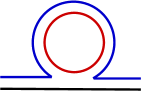
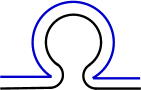
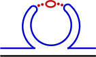
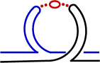
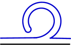
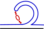
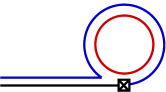
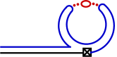
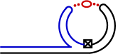
Figure 1: Quark flows for the NLO self-energy tadpoles (a-f) and current-vertex loops (g-i). The $x$ and $y$ quarks are continuously connected to the external lines, closed loops are sea quarks, and current insertions are represented by crossed boxes.

III Next-to-leading order corrections to masses

For a taste $t$ PGB $\phi^{t}_{xy}$ composed of quarks with flavors $x,y,\ x\neq y$, the mass is defined in terms of the self-energy, as in continuum ChPT. The NLO mass can be obtained by adding the NLO self-energy to the tree-level mass,

$$M_{xy,\,t}^{2}=m_{xy,\,t}^{2}+\Sigma_{xy,\,t}(-m_{xy,\,t}^{2})\,.$$ (30)

$\Sigma_{xy,\,t}$ consists of connected and disconnected tadpole loops with vertices from the LO Lagrangian at $\mathcal{O}(\phi^{4})$ and tree-level graphs with vertices from the NLO Lagrangian at $\mathcal{O}(\phi^{2})$. The tadpole graphs contribute the leading chiral logarithms, while the tree-level terms are analytic in the quark masses and the square of the lattice spacing.

We have not attempted to enumerate all terms in the NLO Lagrangian. It consists of generalizations of the Gasser-Leutwyler terms Gasser and Leutwyler (1985), as in ordinary, unmixed SChPT, as well as generalizations of the Sharpe-Van de Water Lagrangian Sharpe and Van de Water (2005) to the mixed action case. There also exist additional operators including traces over taste-singlets; such operators vanish in the unmixed theory.

Given the different kinds of operators in the NLO Lagrangian, the analytic terms at NLO have the same form as those in the unmixed theory, but with distinct LECs for valence-valence, sea-sea, and valence-sea PGBs. Explicitly, we have

$$\Sigma {}^{\mathrm{NLO,\,anal}}_{xy,\,t}(-m_{xy,\,t}^{2})=\frac{16}{f^{2}}\Big{(}(2L_{6}-L_{4})\mu(m_{x}+m_{y})$$ (31)

$$\times\ 2\mu(m_{u}+m_{d}+m_{s})+(2L_{8}-L_{5})[2\mu(m_{x}+m_{y})]^{2}\Big{)}$$

$$+\ c_{1,t}^{xy}a^{2}\mu(m_{x}+m_{y})+c_{2,t}^{xy}a^{2}2\mu(m_{u}+m_{d}+m_{s})$$

$$+\ c_{3,t}^{xy}a^{4}\,,$$

where the coefficients of the last three terms are linear combinations of the LECs in the generalized Sharpe-Van de Water Lagrangian, and so depend on the sector of the $x$ and $y$ quarks: $c_{i,t}^{xy}=c_{i,t}^{vv},\ c_{i,t}^{v\sigma},\ c_{i,t}^{\sigma\sigma}$ for valence-valence, valence-sea, and sea-sea mesons, respectively. We note that for the NLO tree-level diagrams, the symmetry between $x$ and $y$ quarks $x\leftrightarrow y$ is present, as for the ordinary, unmixed case.

A few operators from the Sharpe-Van de Water Lagrangian suffice to justify these claims. We introduce projection operators onto the valence and sea sectors in these operators, lift the degeneracy of the LECs in the three sectors, and calculate the analytic contributions to the self-energies. For example, for first operator in Table 1, we have

$$a^{2}C^{vv}\textrm{Tr}(P_{v}\partial_{\mu}\Sigma^{\dagger}\xi_{5}P_{v}\partial_{\mu}\Sigma\xi_{5})+(v\rightarrow\sigma)$$ (32)

$$+\ a^{2}C^{v\sigma}\left[\textrm{Tr}(P_{v}\partial_{\mu}\Sigma^{\dagger}\xi_{5}P_{\sigma}\partial_{\mu}\Sigma\xi_{5})+p.c.\right]\,,$$

which yield analytic contributions of the form

$$a^{2}\theta^{t5}C^{xy}p^{2}\,,$$ (33)

where the coefficient $C^{xy}=C^{vv},\ C^{\sigma\sigma},\ C^{v\sigma}$ for $xy\in vv,\ \sigma\sigma,\ v\sigma$, and setting $p^{2}=-\mu(m_{x}+m_{y})-a^{2}\Delta_{t}^{xy}$ yields terms like $c_{1,t}^{xy}$ and $c_{3,t}^{xy}$.

Operator	Order
$\textrm{Tr}(\partial_{\mu}\Sigma^{\dagger}\xi_{5}\partial_{\mu}\Sigma\xi_{5})$	$a^{2}p^{2}$
$\textrm{Tr}(\xi_{\mu}\Sigma^{\dagger}\xi_{\mu}\Sigma^{\dagger})\textrm{Tr}(\Sigma M^{\dagger})+p.c.$	$a^{2}m$
$\textrm{Tr}(\xi_{5}\Sigma\xi_{5}\Sigma^{\dagger})\textrm{Tr}(\xi_{5}\Sigma\xi_{5}\Sigma^{\dagger})$	$a^{4}$

Table 1: Examples of operators in the Sharpe-Van de Water Lagrangian contributing tree-level terms to the masses and decay constants at NLO. Such operators enter with undetermined LECs that differ in the valence-valence, valence-sea, and sea-sea sectors, breaking degeneracies between valence and sea quarks.

Finally, we have calculated the tadpole graphs for the sea-sea PGBs and find them identical to the results in the unmixed theory, as expected Bernard and Golterman (1994). Below we consider the tadpole graphs for the valence-valence and valence-sea PGBs.

III.1 Valence-valence sector

For any $\Gamma_{4}\rtimes\,$SO(4) irrep, the calculation of the valence-valence PGB self-energies proceeds as for the unmixed case Aubin and Bernard (2003a); Bailey et al. (2012b). Quark flow diagrams corresponding to the tadpole graphs are shown in diagrams (a-f) of Fig. 1. The kinetic energy, mass, and $\mathcal{U}$ vertices yield graphs of types (a), (c), and (d), and the taste-singlet potential vertices ($\propto C_{\mathrm{mix}}$) yield graphs of type (a),

$$\frac{a^{2}C_{\mathrm{mix}}}{3f^{2}(4\pi f)^{2}}\,\sum_{\overline{i}^{\prime}\underline{i}^{\prime}b}\,\ell(m^{2}_{\overline{i}^{\prime}\underline{i}^{\prime},\,b})\,,$$ (34)

where $\overline{i}^{\prime}$ is summed over $\overline{x},\overline{y}$; $\underline{i}^{\prime}$ is summed over the physical sea quarks $u,d,s$; and $\ell(m^{2})\equiv m^{2}\ln(m^{2}/\Lambda^{2})+\delta_{1}(mL)$ is the chiral logarithm, with $\Lambda$ the scale of dimensional regularization and $\delta_{1}$ the correction for finite spatial volume Bernard (2002). ($L$ is the spatial extent of the lattice.)

Vertices from $\mathcal{U}^{\prime}$ yield graphs of types (b), (e), and (f). The hairpin vertex graphs are of types (e) and (f). As in the unmixed case, they can be combined and eliminated in favor of a contribution of type (d). In the mixed-action case, the necessary identity is ($t\in V,A$)

$$\frac{\delta^{vv}_{F}}{p^{2}+m_{\overline{x}\overline{x},\,t}^{2}}+\frac{\delta^{v\sigma}_{F}}{4}\sum_{\underline{i}^{\prime}}D^{t}_{\overline{x}\underline{i}^{\prime}}=-(p^{2}+m_{\overline{y}\overline{y},\,t}^{2})D^{t}_{\overline{x}\overline{y}}\,.$$ (35)

This relation follows from Eqs. (25) and (26).

As in the unmixed theory, graphs of type (b) come from vertices $\propto\omega^{vv}_{t}\equiv 16(C^{vv}_{2F}+C^{vv}_{5F})/f^{2}$ for $F=V,A$; they have the same form as those in the unmixed case Bailey et al. (2012b).

Adding the various contributions and evaluating the result at $p^{2}=-m^{2}_{\overline{x}\overline{y},\,t}$, we have the NLO, one-loop contributions to the self-energies of the valence-valence PGBs,

$$-\Sigma {}^{\text{NLO loop}}_{\overline{x}\overline{y},\,t}(-m^{2}_{\overline{x}\overline{y},\,t})=\frac{a^{2}}{48(4\pi f)^{2}}\ \times$$ (36)

$$\sum_{c}\Biggl{[} \left(\Delta^{vv,v\sigma}_{ct}-\Delta^{vv}_{t}-\Delta^{v\sigma}_{c}+\frac{16C_{\mathrm{mix}}}{f^{2}}\right)\,\sum_{\overline{i}^{\prime}\underline{i}^{\prime}}\ell(m^{2}_{\overline{i}^{\prime}\underline{i}^{\prime},\,c})$$

$$+\ \frac{3}{2}\Biggl{(}\sum_{b\in V,A}\omega^{vv}_{b}\tau_{cbt}\tau_{cbt}(1+\theta^{ct})\Biggr{)}\ell(m^{2}_{\overline{x}\overline{y},\,c})\Biggr{]}$$

$$+\ \frac{1}{12(4\pi f)^{2}}\,\int\frac{d^{4}q}{\pi^{2}}\ \times$$

$$\sum_{c}\Biggl{[} a^{2}\left(\Delta^{vv}_{ct}-\Delta^{vv}_{t}-\Delta^{vv}_{c}\right)(D_{\overline{xx}}^{c}+D_{\overline{yy}}^{c})$$

$$+\biggl{[} \Bigl{(}2(1-\theta^{ct})+\rho^{ct}\Bigr{)}q^{2}+\Bigl{(}2(1+2\theta^{ct})+\rho^{ct}\Bigr{)}m^{2}_{\overline{x}\overline{y},\,5}$$

$$+\ 2a^{2}\Delta^{\prime vv}_{ct}+a^{2}\Bigl{(}2\theta^{ct}\Delta^{vv}_{t}+(2+\rho^{ct})\Delta^{vv}_{c}\Bigr{)}\biggr{]}D_{\overline{x}\overline{y}}^{c}\Biggr{]}\,,$$

where $\rho^{ct}\equiv-4(2+\theta^{ct})$ unless $c=I$, when it vanishes, $\tau_{cbt}\equiv\textrm{Tr}(T^{c}T^{b}T^{t})$ is a trace over (a product of) generators of U(4), and

$$\Delta^{vv}_{ct} \equiv\frac{8}{f^{2}}\sum_{b\neq I}C^{vv}_{b}(5+3\theta^{cb}\theta^{bt}-4\theta^{5b}\theta^{bt}-4\theta^{cb}\theta^{b5})\,,$$ (37)

$$\Delta^{\prime vv}_{ct} \equiv\frac{8\theta^{ct}}{f^{2}}\sum_{b\neq I}C^{vv}_{b}(1+3\theta^{cb}\theta^{bt}-2\theta^{5b}\theta^{bt}-2\theta^{cb}\theta^{b5})\,,$$ (38)

$$\Delta^{vv,v\sigma}_{ct} \equiv\frac{8}{f^{2}}\sum_{b\neq I}\bigl{[}\tfrac{1}{2}(9C^{vv}_{b}+C^{\sigma\sigma}_{b})+C^{v\sigma}_{b}(3\theta^{cb}\theta^{bt}$$

$$-\ 4\theta^{cb}\theta^{b5})-4C^{vv}_{b}\theta^{5b}\theta^{bt}\bigr{]}\,.$$ (39)

The form of Eq. (36) is the same as that in ordinary SChPT Bailey et al. (2012b); the differences are in the definition of the disconnected propagators and the LECs of the effective field theory. The reduction to the unmixed case is straightforward.

To illustrate the final results, we consider the pions of the 2+1 flavor theory in the fully dynamical case. The theory has two degenerate light quarks and one strange quark in valence and sea sectors, with valence and sea quark masses equal, for each flavor. Substituting for the quark masses in Eq. (36), noting the degeneracies within each $\Gamma_{4}\rtimes\,$SO(4) irrep, summing over the taste index $c$, and performing the loop integrals, we have

$$-\Sigma {}^{\text{NLO loop}}_{\pi^{vv}_{t}}(-m^{2}_{\pi^{vv}_{t}})=\frac{a^{2}}{(4\pi f)^{2}}\ \times$$ (40)

$$\sum_{B}\biggl{[} \delta^{vv,vv}_{BF}\ell(\pi^{vv}_{B})+\frac{\Delta^{vv,v\sigma}_{BF}}{24}\left(2\ell(\pi^{v\sigma}_{B})+\ell(K^{v\sigma}_{B})\right)\biggr{]}$$

$$+\ \frac{1}{12(4\pi f)^{2}}\,\times$$

$$\Biggl{[} 2\sum_{X}\left(12\pi_{P}-6\nu_{VF}X_{V}-a^{2}(\Delta^{vv,vv}_{VF}+\Delta^{\prime\,vv,vv}_{VF})\right)$$

$$\times\ (\delta^{v\sigma}_{V})^{2}/\delta^{\sigma\sigma}_{V}\,\Bigl{[}R^{S^{\sigma\sigma}}_{\pi^{vv}\eta^{\sigma\sigma}\eta^{\prime\,\sigma\sigma}}(X_{V})$$

$$+\ a^{2}(\Delta^{\sigma\sigma}_{V}-\Delta^{vv}_{V})D^{S^{\sigma\sigma}}_{\pi^{vv}\eta^{\sigma\sigma}\eta^{\prime\,\sigma\sigma},\pi^{vv}}(X_{V})\Bigr{]}\ell(X_{V})$$

$$+\ 2\Bigl{[}(\delta^{v\sigma}_{V})^{2}/\delta^{\sigma\sigma}_{V}\,a^{2}(\Delta^{\sigma\sigma}_{V}-\Delta^{vv}_{V})R^{S^{\sigma\sigma}}_{\pi^{vv}\eta^{\sigma\sigma}\eta^{\prime\,\sigma\sigma}}(\pi^{vv}_{V})$$

$$+\ \delta^{vv}_{V}-(\delta^{v\sigma}_{V})^{2}/\delta^{\sigma\sigma}_{V}\Bigr{]}\Bigl{(}6\nu_{VF}\ell(\pi^{vv}_{V})$$

$$+\ \left(12\pi_{P}-6\nu_{VF}\pi^{vv}_{V}-a^{2}(\Delta^{vv,vv}_{VF}+\Delta^{\prime\,vv,vv}_{VF})\right)\tilde{\ell}(\pi^{vv}_{V})\Bigr{)}$$

$$+\ (V\rightarrow A)$$

$$-\ \tfrac{8}{3}\left(3\pi_{P}+2a^{2}\Delta^{vv,vv}_{IF}\right)\biggl{[}\sum_{X}\Bigl{[}R^{S^{\sigma\sigma}}_{\pi^{vv}\eta^{\sigma\sigma}}(X_{I})$$

$$+\ a^{2}(\Delta^{\sigma\sigma}_{I}-\Delta^{vv}_{I})D^{S^{\sigma\sigma}}_{\pi^{vv}\eta^{\sigma\sigma},\pi^{vv}}(X_{I})\Bigr{]}\ell(X_{I})$$

$$+\ a^{2}(\Delta^{\sigma\sigma}_{I}-\Delta^{vv}_{I})R^{S^{\sigma\sigma}}_{\pi^{vv}\eta^{\sigma\sigma}}(\pi^{vv}_{I})\tilde{\ell}(\pi^{vv}_{I})\biggr{]}\Biggr{]}\,.$$

On the right side of Eq. (40), we represent the squares of the tree-level masses by the names of the respective mesons,

$$\pi^{vv}_{B} \equiv 2\mu m_{\ell}+a^{2}\Delta^{vv}_{B}\,,$$ (41)

$$\pi^{v\sigma}_{B} \equiv 2\mu m_{\ell}+a^{2}\Delta^{v\sigma}_{B}\,,$$ (42)

$$K^{v\sigma}_{B} \equiv\mu(m_{\ell}+m_{s})+a^{2}\Delta^{v\sigma}_{B}\,,$$ (43)

$$\pi_{P} \equiv 2\mu m_{\ell}\,,$$ (44)

$$S^{\sigma\sigma}_{B} \equiv 2\mu m_{s}+a^{2}\Delta^{\sigma\sigma}_{B}\,,$$ (45)

and we define linear combinations of LECs that are degenerate within irreps of $\Gamma_{4}\rtimes$SO(4).

$$\delta^{vv,vv}_{BF} \equiv\sum_{c\in B}\frac{1}{32}\Biggl{(}\sum_{b\in V,A}\omega^{vv}_{b}\tau_{cbt}\tau_{cbt}(1+\theta^{ct})\Biggr{)}\,,$$ (46)

$$\Delta^{vv,v\sigma}_{BF} \equiv\sum_{c\in B}\left(\Delta^{vv,v\sigma}_{ct}-\Delta^{vv}_{t}-\Delta^{v\sigma}_{c}+\frac{16C_{\mathrm{mix}}}{f^{2}}\right)\,,$$ (47)

$$\Delta^{vv,vv}_{BF} \equiv\sum_{c\in B}\left(\Delta^{vv}_{ct}-\Delta^{vv}_{t}-\Delta^{vv}_{c}\right)\,,$$ (48)

$$\Delta^{\prime vv,vv}_{BF} \equiv\sum_{c\in B}\left(\Delta^{\prime vv}_{ct}+\Bigl{(}\theta^{ct}\Delta^{vv}_{t}+(1+\rho^{ct}/2)\Delta^{vv}_{c}\Bigr{)}\right)\,.$$ (49)

The whole number $\nu_{BF}\equiv\tfrac{1}{2}\sum_{c\in B}(1+\theta^{ct})$ counts the taste matrices in irrep $B$ commuting with the taste matrix $\xi_{t}$, where $t\in F$. The index of summation $X$ runs over the meson names in the subscripts of the residues, which are defined as in Ref. Bailey et al. (2012b),

$$R^{A_{1}A_{2}\cdots A_{k}}_{B_{1}B_{2}\cdots B_{n}}(X_{F}) \equiv\frac{\prod_{A_{jF}}(A_{jF}-X_{F})}{\prod_{B_{iF}\neq X_{F}}(B_{iF}-X_{F})}\,,$$ (50)

$$D^{A_{1}A_{2}\cdots A_{k}}_{B_{1}B_{2}\cdots B_{n},B_{i}}(X_{F}) \equiv-\frac{\partial}{\partial B_{iF}}R^{A_{1}A_{2}\cdots A_{k}}_{B_{1}B_{2}\cdots B_{n}}(X_{F})\,.$$ (51)

The chiral behavior of the mixed action theory differs nontrivially from that of the unmixed theory due to incomplete cancellation of double poles in the loop integrals. The chiral logarithm $\tilde{\ell}(m^{2})\equiv-(\ln(m^{2}/\Lambda^{2})+1)+\delta_{3}(mL)$, with the finite volume correction $\delta_{3}$ Bernard (2002), arises from these loops. Unlike in the ordinary theory, such terms enter here even though valence and sea quark masses for each flavor are equal, i.e., in the fully dynamical case.

The valence-valence, taste-pseudoscalar PGBs are true Goldstone bosons in the chiral limit, $m_{x},m_{y}\rightarrow 0,\ a\neq 0$. Setting $t=5$ in Eq. (36) and noting that

$$\Delta^{vv,v\sigma}_{c5} =\Delta^{v\sigma}_{c}-\frac{16C_{\mathrm{mix}}}{f^{2}}$$ (52)

$$\Delta^{vv}_{c5} =\Delta^{vv}_{c}$$ (53)

$$\Delta^{\prime vv}_{c5} =-\theta^{c5}\Delta^{vv}_{c}$$ (54)

$$\Delta^{vv}_{5} =0\,,$$ (55)

we have

$$-\Sigma^{\text{NLO loop}}_{\overline{x}\overline{y},\,5}(-m^{2}_{\overline{x}\overline{y},\,5})=\frac{\mu(m_{\overline{x}}+m_{\overline{y}})}{2(4\pi f)^{2}}\,\sum_{b}\theta^{b5}\int\frac{d^{4}q}{\pi^{2}}D^{b}_{\overline{x}\overline{y}}\,,$$ (56)

which is the generalization of the results of Ref. Aubin and Bernard (2003a) to the mixed-action case. As in ordinary SChPT, only graphs of type (d) contribute. To generalize to the mixed-action theory, one has only to replace the disconnected propagators $D^{t}_{\overline{x}\overline{y}}$ with their counterparts in the mixed-action theory.

III.2 Valence-sea sector

We consider mesons $\phi^{t}_{\overline{x}\underline{y}}$ with one valence quark $\overline{x}$ and one sea quark $\underline{y}$. For tadpoles with vertices from the kinetic energy and mass terms of the LO Lagrangian (Eq. (4)), we find graphs of types (a), (c), and (d).

$$\frac{1}{48(4\pi f)^{2}}\,\sum_{c,\underline{i}^{\prime}}\Bigg{[}\left(p^{2}+\mu(m_{\overline{x}}+m_{\underline{y}})-a^{2}\Delta^{v\sigma}_{c}\right)\ell(m^{2}_{\overline{x}\underline{i}^{\prime},c})$$ (57)

$$+\ \left(p^{2}+\mu(m_{\overline{x}}+m_{\underline{y}})-a^{2}\Delta^{\sigma\sigma}_{c}\right)\ell(m^{2}_{\underline{y}\underline{i}^{\prime},c})\Bigg{]}$$

$$+\ \frac{1}{12(4\pi f)^{2}}\,\sum_{c}\int\frac{d^{4}q}{\pi^{2}}\Biggl{[}\left(p^{2}+q^{2}+\mu(3m_{\overline{x}}+m_{\underline{y}})\right)D^{c}_{\overline{x}\overline{x}}$$

$$+\ \left(p^{2}+q^{2}+\mu(m_{\overline{x}}+3m_{\underline{y}})\right)D^{c}_{\underline{y}\underline{y}}$$

$$-\ 2\theta^{ct}\left(p^{2}+q^{2}-\mu(m_{\overline{x}}+m_{\underline{y}})\right)D_{\overline{x}\underline{y}}^{c}\Biggr{]}\,,$$

where $\underline{i}^{\prime}$ is summed over the physical sea-quark flavors. As for the sea-sea and valence-valence sectors, the $q^{2}D^{c}_{\overline{x}\overline{x}}$ and $q^{2}D^{c}_{\underline{y}\underline{y}}$ terms can be eliminated in favor of a $q^{2}D^{c}_{\overline{x}\underline{y}}$ term. But for the valence-sea mesons, an additional term arises, with the form of a connected contribution [graph (e) of Fig. 1]. The necessary identities are

$$(q^{2}+2\mu m_{\overline{x}})D^{t}_{\overline{x}\overline{x}} =\frac{\delta^{v\sigma}_{F}}{\delta^{\sigma\sigma}_{F}}(q^{2}+m_{\underline{yy},\,t}^{2})D^{t}_{\overline{x}\underline{y}}$$ (58)

$$-\,a^{2}\Delta^{vv}_{F}D^{t}_{\overline{x}\overline{x}}+\frac{(\delta^{v\sigma}_{F})^{2}/\delta^{\sigma\sigma}_{F}-\delta^{vv}_{F}}{q^{2}+m_{\overline{xx},\,t}^{2}}\,,$$

$$(q^{2}+2\mu m_{\underline{y}})D^{t}_{\underline{y}\underline{y}} =\frac{\delta^{\sigma\sigma}_{F}}{\delta^{v\sigma}_{F}}(q^{2}+m_{\overline{xx},\,t}^{2})D^{t}_{\overline{x}\underline{y}}$$ (59)

$$-\,a^{2}\Delta^{\sigma\sigma}_{F}D^{t}_{\underline{y}\underline{y}}\,,$$

which hold for $t\in F=V,A,I$. Applying these identities to the above result gives

$$\frac{1}{48(4\pi f)^{2}}\,\sum_{c,\underline{i}^{\prime}}\Bigg{[} \left(p^{2}+\mu(m_{\overline{x}}+m_{\underline{y}})-a^{2}\Delta^{v\sigma}_{c}\right)\ell(m^{2}_{\overline{x}\underline{i}^{\prime},c})$$ (60)

$$+\ \left(p^{2}+\mu(m_{\overline{x}}+m_{\underline{y}})-a^{2}\Delta^{\sigma\sigma}_{c}\right)\ell(m^{2}_{\underline{y}\underline{i}^{\prime},c})\Bigg{]}$$

$$-\ \frac{1}{12(4\pi f)^{2}} \sum_{c\in V,A}\left(\delta^{vv}_{c}-(\delta^{v\sigma}_{c})^{2}/\delta^{\sigma\sigma}_{c}\right)\ell(m^{2}_{\overline{x}\overline{x},c})$$

$$+\ \frac{1}{12(4\pi f)^{2}} \sum_{c}\int\frac{d^{4}q}{\pi^{2}}\ \times$$

$$\Biggl{[} \left(p^{2}+\mu(m_{\overline{x}}+m_{\underline{y}})-a^{2}\Delta^{vv}_{c}\right)D^{c}_{\overline{x}\overline{x}}$$

$$+\ \left(p^{2}+\mu(m_{\overline{x}}+m_{\underline{y}})-a^{2}\Delta^{\sigma\sigma}_{c}\right)D^{c}_{\underline{y}\underline{y}}$$

$$+\ \Biggl{(}-2\theta^{ct}p^{2}+\left(\frac{\delta^{v\sigma}_{c}}{\delta^{\sigma\sigma}_{c}}+\frac{\delta^{\sigma\sigma}_{c}}{\delta^{v\sigma}_{c}}-2\theta^{ct}\right)q^{2}$$

$$+\left(\frac{\delta^{\sigma\sigma}_{c}}{\delta^{v\sigma}_{c}}+\theta^{ct}\right) (2\mu m_{\overline{x}})+\left(\frac{\delta^{v\sigma}_{c}}{\delta^{\sigma\sigma}_{c}}+\theta^{ct}\right)(2\mu m_{\underline{y}})$$

$$+\ a^{2}\left(\frac{\delta^{v\sigma}_{c}}{\delta^{\sigma\sigma}_{c}}\Delta^{\sigma\sigma}_{c}+\frac{\delta^{\sigma\sigma}_{c}}{\delta^{v\sigma}_{c}}\Delta^{vv}_{c}\right)\Biggr{)}D_{\overline{x}\underline{y}}^{c}\Biggr{]}\,.$$

From the taste-singlet potential, we find contributions not only from graphs of type (a), as in the valence-valence sector, but also from graphs of types (c) and (d),

$$\frac{a^{2}C_{\mathrm{mix}}}{3f^{2}(4\pi f)^{2}}\,\sum_{b}\Bigg{[}\sum_{\underline{i}^{\prime}}\left(8\ell(m^{2}_{\overline{x}\underline{i}^{\prime},b})+\ell(m^{2}_{\underline{y}\underline{i}^{\prime},b})\right)$$ (61)

$$+\ 4\int\frac{d^{4}q}{\pi^{2}}\left(D^{b}_{\overline{x}\overline{x}}+D^{b}_{\underline{y}\underline{y}}-2\theta^{bt}D_{\overline{x}\underline{y}}^{b}\right)\Bigg{]}\,.$$

From the single-trace potential $\mathcal{U}$, we have graphs of types (a), (c), and (d),

$$\frac{a^{2}}{48(4\pi f)^{2}}\sum_{b}\Bigg{[}\sum_{\underline{i}^{\prime}}\Big{(}\Delta_{bt}^{v\sigma,v\sigma}\ell(m^{2}_{\overline{x}\underline{i}^{\prime},b})$$ (62)

$$+\ \Delta_{bt}^{v\sigma,\sigma\sigma}\ell(m^{2}_{\underline{y}\underline{i}^{\prime},b})\Big{)}$$

$$+\ 4\int\frac{d^{4}q}{\pi^{2}}\Big{(}\Delta_{bt}^{v\sigma,vv}D^{b}_{\overline{x}\overline{x}}+\Delta_{bt}^{v\sigma,\sigma\sigma}D^{b}_{\underline{y}\underline{y}}$$

$$+\ 2\Delta_{bt}^{\prime\,v\sigma,v\sigma}D_{\overline{x}\underline{y}}^{b}\Big{)}\Bigg{]}\,,$$

where

$$\Delta_{ct}^{v\sigma,v\sigma}\equiv\frac{8}{f^{2}}\sum_{b\neq I} \bigl{[}4C^{vv}_{b}+C^{\sigma\sigma}_{b}\bigl{(}1+3\theta^{cb}\theta^{bt}\bigr{)}$$ (63)

$$-\ 4C^{v\sigma}_{b}\bigl{(}\theta^{5b}\theta^{bt}+\theta^{cb}\theta^{b5}\bigr{)}\bigr{]}\,,$$

$$\Delta_{ct}^{v\sigma,\sigma\sigma}\equiv\frac{8}{f^{2}}\sum_{b\neq I} \bigl{[}C^{\sigma\sigma}_{b}\bigl{(}\tfrac{9}{2}-4\theta^{cb}\theta^{b5}\bigr{)}+\tfrac{1}{2}C^{vv}_{b}$$ (64)

$$+\ C^{v\sigma}_{b}\bigl{(}3\theta^{cb}\theta^{bt}-4\theta^{5b}\theta^{bt}\bigr{)}\bigr{]}\,,$$

$$\Delta_{ct}^{v\sigma,vv}\equiv\frac{8}{f^{2}}\sum_{b\neq I} \bigl{[}C^{vv}_{b}\bigl{(}\tfrac{9}{2}-4\theta^{cb}\theta^{b5}\bigr{)}+\tfrac{1}{2}C^{\sigma\sigma}_{b}$$ (65)

$$+\ C^{v\sigma}_{b}\bigl{(}3\theta^{cb}\theta^{bt}-4\theta^{5b}\theta^{bt}\bigr{)}\bigr{]}\,,$$

$$\Delta_{ct}^{\prime\,v\sigma,v\sigma}\equiv\frac{8\theta^{ct}}{f^{2}}\sum_{b\neq I} \bigl{[}\bigl{(}C^{vv}_{b}+C^{\sigma\sigma}_{b}\bigr{)}\bigl{(}\tfrac{1}{2}-\theta^{cb}\theta^{b5}\bigr{)}$$ (66)

$$+\ C^{v\sigma}_{b}\bigl{(}3\theta^{cb}\theta^{bt}-2\theta^{5b}\theta^{bt}\bigr{)}\bigr{]}\,.$$

In the unmixed case, $\Delta_{ct}^{v\sigma,v\sigma}=\Delta_{ct}^{v\sigma,\sigma\sigma}=\Delta_{ct}^{v\sigma,vv}=\Delta_{ct}$, $\Delta_{ct}^{\prime\,v\sigma,v\sigma}=\Delta_{ct}^{\prime}$, and the contribution from $\mathcal{U}$ reduces Aubin and Bernard (2003a); Bailey et al. (2012b). We note that $\Delta_{ct}^{v\sigma,\sigma\sigma}$ appears in both connected and disconnected terms.

From the double-trace potential $\mathcal{U}^{\prime}$, we have, after combining graphs of types (e) and (f) to eliminate those of type (f),

$$\frac{1}{12(4\pi f)^{2}}\ \times$$ (67)

$$\sum_{c}\biggl{[} \frac{3a^{2}}{8}\sum_{b\in V,A}\tau_{cbt}\tau_{cbt}\left(\omega^{v\sigma}_{b}+\frac{\theta^{ct}}{2}(\omega^{vv}_{b}+\omega^{\sigma\sigma}_{b})\right)\ell(m_{\overline{x}\underline{y},\,c}^{2})$$

$$+ \int\frac{d^{4}q}{\pi^{2}}\rho^{ct}\left(q^{2}+m_{\overline{x}\underline{y},\,5}^{2}+\frac{a^{2}}{2}(\Delta^{vv}_{c}+\Delta^{\sigma\sigma}_{c})\right)D^{c}_{\overline{x}\underline{y}}\biggr{]}$$

$$+\ \frac{1}{3(4\pi f)^{2}}\sum_{c\in V,A}\biggl{[}\Bigl{(}\delta^{vv}_{c}-(\delta^{v\sigma}_{c})^{2}/\delta^{\sigma\sigma}_{c}\Bigr{)}\ell(m^{2}_{\overline{xx},c})$$

$$+ \int\frac{d^{4}q}{\pi^{2}}\biggl{(}\Bigl{(}2-\delta^{\sigma\sigma}_{c}/\delta^{v\sigma}_{c}-\delta^{v\sigma}_{c}/\delta^{\sigma\sigma}_{c}\Bigr{)}q^{2}$$

$$+\ \Bigl{(}1-\delta^{\sigma\sigma}_{c}/\delta^{v\sigma}_{c}\Bigr{)}(2\mu m_{\overline{x}}+a^{2}\Delta^{vv}_{c})$$

$$+\ \Bigl{(}1-\delta^{v\sigma}_{c}/\delta^{\sigma\sigma}_{c}\Bigr{)}(2\mu m_{\underline{y}}+a^{2}\Delta^{\sigma\sigma}_{c})\biggr{)}D^{c}_{\overline{x}\underline{y}}\biggr{]}\,.$$

The reduction of this expression in the unmixed case is immediate. In the valence-valence sector and unmixed cases, the graphs of types (e) and (f) can be combined into a graph of type (d). In the valence-sea sector, we eliminate graphs of type (f) in favor of those of type (d), but a contribution of type (e) remains.

Adding the various contributions and evaluating the sum at $p^{2}=-m^{2}_{\overline{x}\underline{y},\,t}$ gives, for graphs with connected propagators,

$$-\Sigma {}_{\overline{x}\underline{y},\,t}^{\mathrm{NLO\ loop,\ con}}(-m^{2}_{\overline{x}\underline{y},t})=\frac{a^{2}}{48(4\pi f)^{2}}\ \times$$ (68)

$$\sum_{c}\Bigg{[} \left(\Delta_{ct}^{v\sigma,v\sigma}-\Delta^{v\sigma}_{t}-\Delta^{v\sigma}_{c}+\frac{128C_{\text{mix}}}{f^{2}}\right)\sum_{\underline{i}^{\prime}}\ell(m^{2}_{\overline{x}\underline{i}^{\prime},c})$$

$$+\ \left(\Delta_{ct}^{v\sigma,\sigma\sigma}-\Delta^{v\sigma}_{t}-\Delta^{\sigma\sigma}_{c}+\frac{16C_{\text{mix}}}{f^{2}}\right)\sum_{\underline{i}^{\prime}}\ell(m^{2}_{\underline{y}\underline{i}^{\prime},c})$$

$$+\ \frac{3}{2}\sum_{b\in V,A}\tau_{cbt}\tau_{cbt}\left(\omega_{b}^{v\sigma}+\frac{\theta^{ct}}{2}(\omega_{b}^{vv}+\omega_{b}^{\sigma\sigma})\right)\ell(m^{2}_{\overline{x}\underline{y},c})\Bigg{]}$$

$$+\ \frac{1}{4(4\pi f)^{2}}\sum_{c\in V,A}\left(\delta^{vv}_{c}-(\delta^{v\sigma}_{c})^{2}/\delta^{\sigma\sigma}_{c}\right)\ell(m^{2}_{\overline{x}\overline{x},c})\,,$$

while for the graphs with disconnected propagators, we have

$$-\Sigma {}_{\overline{x}\underline{y},\,t}^{\mathrm{NLO\ loop,\ disc}}(-m^{2}_{\overline{x}\underline{y},t})=\ \frac{1}{12(4\pi f)^{2}}\int\frac{d^{4}q}{\pi^{2}}\ \times$$ (69)

$$\sum_{c}\Biggl{[} a^{2}\left(\Delta_{ct}^{v\sigma,vv}-\Delta^{v\sigma}_{t}-\Delta^{vv}_{c}+\frac{16C_{\text{mix}}}{f^{2}}\right)D^{c}_{\overline{x}\overline{x}}$$

$$+\ a^{2}\left(\Delta_{ct}^{v\sigma,\sigma\sigma}-\Delta^{v\sigma}_{t}-\Delta^{\sigma\sigma}_{c}+\frac{16C_{\text{mix}}}{f^{2}}\right)D^{c}_{\underline{y}\underline{y}}$$

$$+\ \bigg{[}\left(8-3\bigg{(}\frac{\delta^{v\sigma}_{c}}{\delta^{\sigma\sigma}_{c}}+\frac{\delta^{\sigma\sigma}_{c}}{\delta^{v\sigma}_{c}}\bigg{)}-2\theta^{ct}+\rho^{ct}\right)q^{2}$$

$$+\ \left(4-3\frac{\delta^{\sigma\sigma}_{c}}{\delta^{v\sigma}_{c}}+2\theta^{ct}+\frac{\rho^{ct}}{2}\right)(2\mu m_{\overline{x}})$$

$$+\ \left(4-3\frac{\delta^{v\sigma}_{c}}{\delta^{\sigma\sigma}_{c}}+2\theta^{ct}+\frac{\rho^{ct}}{2}\right)(2\mu m_{\underline{y}})+2a^{2}\Delta_{ct}^{\prime\,v\sigma,v\sigma}$$

$$+\ a^{2}\bigg{(}2\theta^{ct}\Delta^{v\sigma}_{t}+\bigg{(}4-3\frac{\delta^{\sigma\sigma}_{c}}{\delta^{v\sigma}_{c}}+\frac{\rho^{ct}}{2}\bigg{)}\Delta^{vv}_{c}$$

$$+\ \bigg{(}4-3\frac{\delta^{v\sigma}_{c}}{\delta^{\sigma\sigma}_{c}}+\frac{\rho^{ct}}{2}\bigg{)}\Delta^{\sigma\sigma}_{c}\bigg{)}-\frac{32a^{2}\theta^{ct}C_{\text{mix}}}{f^{2}}\bigg{]}D_{\overline{x}\underline{y}}^{c}\Biggr{]}\,.$$

The reduction in the unmixed case is straightforward. There is no symmetry under $\overline{x}\leftrightarrow\underline{y}$; when using the replica method, the valence and sea sectors of the effective theory are distinguished by the operations of partial quenching (the valence quarks) and rooting (the sea quarks). The taste-pseudoscalars are not Goldstone bosons (in the chiral limit) at non-zero lattice spacing, and the self-energy does not vanish in the chiral limit. In the continuum limit, the symmetry is restored, and the masses vanish, in accord with Goldstone’s theorem.

To illustrate the final results, we again consider the pions of the 2+1 flavor theory with degenerate valence and sea quarks. We have

$$-\Sigma {}_{\pi^{v\sigma}_{t}}^{\mathrm{NLO\ loop}}(-m^{2}_{\pi^{v\sigma}_{t}})=\frac{a^{2}}{(4\pi f)^{2}}\ \times$$ (70)

$$\sum_{B}\Bigg{[} \delta^{v\sigma,v\sigma}_{BF}\ell(\pi^{v\sigma}_{B})+\frac{\Delta^{v\sigma,v\sigma}_{BF}}{48}\left(2\ell(\pi^{v\sigma}_{B})+\ell(K^{v\sigma}_{B})\right)$$

$$+\ \frac{\Delta^{v\sigma,\sigma\sigma}_{BF}}{48}\left(2\ell(\pi^{\sigma\sigma}_{B})+\ell(K^{\sigma\sigma}_{B})\right)\Bigg{]}$$

$$+\ \frac{1}{(4\pi f)^{2}}\left(\delta^{vv}_{V}-(\delta^{v\sigma}_{V})^{2}/\delta^{\sigma\sigma}_{V}\right)\ell(\pi^{vv}_{V})+(V\rightarrow A)$$

$$+\ \frac{1}{12(4\pi f)^{2}}\ \times$$

$$\Bigg{\{}\delta^{v\sigma}_{V}\sum_{X} \Biggl{[}2\Biggl{(}6\left(\frac{\delta^{\sigma\sigma}_{V}}{\delta^{v\sigma}_{V}}+\frac{\delta^{v\sigma}_{V}}{\delta^{\sigma\sigma}_{V}}\right)\pi_{P}-6\biggl{[}\nu_{VF}$$

$$+\ \left(\frac{\delta^{\sigma\sigma}_{V}}{\delta^{v\sigma}_{V}}+\frac{\delta^{v\sigma}_{V}}{\delta^{\sigma\sigma}_{V}}-2\right)\biggr{]}X_{V}-a^{2}\bigg{(}\frac{\Delta^{v\sigma,vv}_{VF}}{2}\frac{\delta^{v\sigma}_{V}}{\delta^{\sigma\sigma}_{V}}$$

$$+\ \Delta^{\prime v\sigma,v\sigma}_{VF}\bigg{)}\Biggr{)}R^{S^{\sigma\sigma}}_{\pi^{vv}\eta^{\sigma\sigma}\eta^{\prime\,\sigma\sigma}}(X_{V})-\frac{\delta^{v\sigma}_{V}}{\delta^{\sigma\sigma}_{V}}a^{2}\Delta^{v\sigma,vv}_{VF}$$

$$\times\ a^{2}\left(\Delta^{\sigma\sigma}_{V}-\Delta^{vv}_{V}\right)D^{S^{\sigma\sigma}}_{\pi^{vv}\eta^{\sigma\sigma}\eta^{\prime\,\sigma\sigma},\pi^{vv}}(X_{V})\Biggr{]}\ell(X_{V})$$

$$-\ a^{2}\Delta^{v\sigma,\sigma\sigma}_{VF}\delta^{\sigma\sigma}_{V}\sum_{X}R^{S^{\sigma\sigma}}_{\pi^{\sigma\sigma}\eta^{\sigma\sigma}\eta^{\prime\,\sigma\sigma}}(X_{V})\ell(X_{V})$$

$$-\ a^{2}\Delta^{v\sigma,vv}_{VF}\Big{[}(\delta^{v\sigma}_{V})^{2}/\delta^{\sigma\sigma}_{V}a^{2}(\Delta^{\sigma\sigma}_{V}-\Delta^{vv}_{V})$$

$$\times\ R^{S^{\sigma\sigma}}_{\pi^{vv}\eta^{\sigma\sigma}\eta^{\prime\,\sigma\sigma}}(\pi^{vv}_{V})+\delta^{vv}_{V}-(\delta^{v\sigma}_{V})^{2}/\delta^{\sigma\sigma}_{V}\Big{]}\tilde{\ell}(\pi^{vv}_{V})$$

$$+\ (V\rightarrow A)$$

$$-\ \frac{4}{3}\Bigg{[}\left(2(3\pi_{P}+a^{2}\Delta^{v\sigma,vv}_{IF})+a^{2}\Delta^{v\sigma,\sigma\sigma}_{IF}\right)$$

$$\times\ \sum_{X}R^{S^{\sigma\sigma}}_{\pi^{vv}\eta^{\sigma\sigma}}(X_{I})\ell(X_{I})$$

$$+\ a^{2}\Delta^{v\sigma,vv}_{IF}a^{2}(\Delta^{\sigma\sigma}_{I}-\Delta^{vv}_{I})\Big{[}R^{S^{\sigma\sigma}}_{\pi^{vv}\eta^{\sigma\sigma}}(\pi^{vv}_{I})\tilde{\ell}(\pi^{vv}_{I})$$

$$+\ \sum_{X}D^{S^{\sigma\sigma}}_{\pi^{vv}\eta^{\sigma\sigma},\pi^{vv}}(X_{I})\ell(X_{I})\Big{]}$$

$$+\ a^{2}\Delta^{v\sigma,\sigma\sigma}_{IF}\sum_{X}R^{S^{\sigma\sigma}}_{\pi^{\sigma\sigma}\eta^{\sigma\sigma}}(X_{I})\ell(X_{I})\Bigg{]}\Bigg{\}}\,.$$

The new linear combinations of LECs are

$$\delta^{v\sigma,v\sigma}_{BF} \equiv\frac{1}{32}\sum_{c\in B}\sum_{b\in V,A}\tau^{2}_{cbt}\left(\omega^{v\sigma}_{b}+\tfrac{1}{2}\theta^{ct}(\omega^{vv}_{b}+\omega^{\sigma\sigma}_{b})\right)\,,$$ (71)

$$\Delta^{v\sigma,v\sigma}_{BF} \equiv\sum_{c\in B}\left(\Delta^{v\sigma,v\sigma}_{ct}-\Delta^{v\sigma}_{t}-\Delta^{v\sigma}_{c}+\frac{128C_{\mathrm{mix}}}{f^{2}}\right)\,,$$ (72)

$$\Delta^{v\sigma,\sigma\sigma}_{BF} \equiv\sum_{c\in B}\left(\Delta^{v\sigma,\sigma\sigma}_{ct}-\Delta^{v\sigma}_{t}-\Delta^{\sigma\sigma}_{c}+\frac{16C_{\mathrm{mix}}}{f^{2}}\right)\,,$$ (73)

$$\Delta^{v\sigma,vv}_{BF} \equiv\sum_{c\in B}\left(\Delta^{v\sigma,vv}_{ct}-\Delta^{v\sigma}_{t}-\Delta^{vv}_{c}+\frac{16C_{\mathrm{mix}}}{f^{2}}\right)\,,$$ (74)

$$\Delta^{\prime v\sigma,v\sigma}_{BF} \equiv\sum_{c\in B}\bigg{[}\Delta^{\prime v\sigma,v\sigma}_{ct}+\theta^{ct}\Delta^{v\sigma}_{t}+\frac{\Delta^{vv}_{c}}{2}\bigg{(}4-3\frac{\delta^{\sigma\sigma}_{c}}{\delta^{v\sigma}_{c}}$$

$$+\ \frac{\rho^{ct}}{2}\bigg{)}+\frac{\Delta^{\sigma\sigma}_{c}}{2}\bigg{(}4-3\frac{\delta^{v\sigma}_{c}}{\delta^{\sigma\sigma}_{c}}+\frac{\rho^{ct}}{2}\bigg{)}-\frac{16\theta^{ct}C_{\mathrm{mix}}}{f^{2}}\bigg{]}\,,$$ (75)

and we use the identity $\Delta^{\prime v\sigma,v\sigma}_{IF}=\tfrac{1}{2}(\Delta^{v\sigma,vv}_{IF}+\Delta^{v\sigma,\sigma\sigma}_{IF})$ to simplify the disconnected loops in the taste singlet channel. As for the valence-valence masses, the chiral behavior differs nontrivially from that of the ordinary unmixed theory. Even in the fully dynamical theory, double poles do not completely cancel from the loop integrals.

IV Next-to-leading order corrections to decay constants

As for continuum and ordinary SChPT, the decay constants are defined by matrix elements of the axial currents,

$$-if_{xy,\,t}\,p_{\mu}=\langle 0|\,j^{\mu 5}_{xy,\,t}\,|\phi^{t}_{xy}(p)\rangle\,.$$ (76)

The NLO corrections are the same types of diagrams that appear in continuum and unmixed SChPT. We have one-loop wave function renormalization contributions [graphs (a), (c), and (d) of Fig. 1], one-loop graphs from insertions of the $\mathcal{O}(\phi^{3})$-terms of the LO current [graphs (g), (h), and (i) of Fig. 1], and terms analytic in the quark masses and squared lattice spacing, from the NLO Lagrangian Aubin and Bernard (2003b). As for the NLO analytic corrections to the masses, the NLO analytic corrections to the decay constants have the same form as in the unmixed theory, with distinct LECs for the valence-valence, sea-sea, and valence-sea sectors.

Turning to the one-loop corrections, we note that the LO current is determined by the kinetic energy vertices of the LO Lagrangian; these vertices are the same in mixed-action and unmixed SChPT. Therefore, the LO current in the mixed-action case is the same as the LO current in unmixed SChPT. Likewise, the NLO wave function renormalization corrections are determined by self-energy contributions from tadpoles with kinetic energy vertices from the LO Lagrangian. Moreover, nothing in the calculation of the relevant part of the self-energies or the current-vertex loops is sensitive to the sector of the external quarks.

Therefore, to generalize the one-loop graphs of the unmixed case, we have only to replace the propagators with those of the mixed-action theory. The results hold for all sectors of the mixed-action theory (valence-valence, sea-sea, and valence-sea). Including the analytic contributions, we have

$$\frac{f^{\text{NLO}}_{xy,\,t}}{f}=1-\frac{1}{8(4\pi f)^{2}}\sum_{c}\ \times$$ (77)

$$\left[\frac{1}{4}\sum_{\overline{i}^{\prime}\underline{i}^{\prime}}\ell(m^{2}_{\overline{i}^{\prime}\underline{i}^{\prime},\,c})+\int\frac{d^{4}q}{\pi^{2}}(D^{c}_{xx}+D^{c}_{yy}-2\theta^{ct}D^{c}_{xy})\right]$$

$$+\frac{16}{f^{2}}L_{4}\mu(m_{u}+m_{d}+m_{s})+\frac{8}{f^{2}}L_{5}\mu(m_{x}+m_{y})+a^{2}c^{xy}_{t}\,,$$

where the coefficient $c^{xy}_{t}=c^{vv}_{t},\ c^{v\sigma}_{t},\ c^{\sigma\sigma}_{t}$ for valence-valence, valence-sea, and sea-sea mesons, respectively. The form of this result is the same as that in the unmixed theory Bailey et al. (2013), and the reduction in the unmixed case is immediate. As for the masses, the form of the NLO analytic terms can be verified by considering a few operators in the generalized Sharpe-Van de Water Lagrangian and calculating the resulting contributions. In addition to the wave function renormalization contributions, there are those from the NLO current. But the latter cannot change the form of the results, and considering the wave function renormalization suffices.

To illustrate the loop corrections, we begin with the valence-valence pions in the 2+1 flavor, fully dynamical theory. We have

$$\frac{f^{\text{NLO loop}}_{\pi^{vv}_{t}}}{f}=-\frac{1}{16(4\pi f)^{2}}\sum_{B}g_{B}\left(2\ell(\pi^{v\sigma}_{B})+\ell(K^{v\sigma}_{B})\right)$$ (78)

$$+\ \frac{(1-\Theta^{VF}/4)}{(4\pi f)^{2}}\Bigg{[}\sum_{X}(\delta^{v\sigma}_{V})^{2}/\delta^{\sigma\sigma}_{V}\bigg{(}R^{S^{\sigma\sigma}}_{\pi^{vv}\eta^{\sigma\sigma}\eta^{\prime\,\sigma\sigma}}(X_{V})$$

$$+\ a^{2}(\Delta^{\sigma\sigma}_{V}-\Delta^{vv}_{V})D^{S^{\sigma\sigma}}_{\pi^{vv}\eta^{\sigma\sigma}\eta^{\prime\,\sigma\sigma},\pi^{vv}}(X_{V})\bigg{)}\ell(X_{V})$$

$$+\ \Big{[}(\delta^{v\sigma}_{V})^{2}/\delta^{\sigma\sigma}_{V}a^{2}(\Delta^{\sigma\sigma}_{V}-\Delta^{vv}_{V})R^{S^{\sigma\sigma}}_{\pi^{vv}\eta^{\sigma\sigma}\eta^{\prime\,\sigma\sigma}}(\pi^{vv}_{V})$$

$$+\ \left(\delta^{vv}_{V}-(\delta^{v\sigma}_{V})^{2}/\delta^{\sigma\sigma}_{V}\right)\Big{]}\tilde{\ell}(\pi^{vv}_{V})\Bigg{]}+(V\rightarrow A)\,,$$

where $g_{B}\equiv\sum_{c\in B}1$ and $\Theta^{BF}\equiv\sum_{c\in B}\theta^{ct}$, as for the unmixed case. For the valence-sea pions in the 2+1 flavor, fully dynamical theory, we have

$$\frac{f^{\text{NLO loop}}_{\pi^{v\sigma}_{t}}}{f}=-\frac{1}{16(4\pi f)^{2}}\sum_{B}g_{B}\left(2\ell(\pi^{v\sigma}_{B})+\ell(K^{v\sigma}_{B})\right)$$ (79)

$$+\ \frac{1}{2(4\pi f)^{2}}\Bigg{[}\sum_{X}\Bigg{(}\delta^{v\sigma}_{V}\left(\frac{\delta^{v\sigma}_{V}}{\delta^{\sigma\sigma}_{V}}-\frac{\Theta^{VF}}{2}\right)R^{S^{\sigma\sigma}}_{\pi^{vv}\eta^{\sigma\sigma}\eta^{\prime\,\sigma\sigma}}(X_{V})$$

$$+\ \frac{(\delta^{v\sigma}_{V})^{2}}{\delta^{\sigma\sigma}_{V}}a^{2}(\Delta^{\sigma\sigma}_{V}-\Delta^{vv}_{V})D^{S^{\sigma\sigma}}_{\pi^{vv}\eta^{\sigma\sigma}\eta^{\prime\,\sigma\sigma},\pi^{vv}}(X_{V})\Bigg{)}\ell(X_{V})$$

$$+\ \delta^{\sigma\sigma}_{V}\sum_{X}R^{S^{\sigma\sigma}}_{\pi^{\sigma\sigma}\eta^{\sigma\sigma}\eta^{\prime\,\sigma\sigma}}(X_{V})\ell(X_{V})$$

$$+\ \Big{[}(\delta^{v\sigma}_{V})^{2}/\delta^{\sigma\sigma}_{V}a^{2}(\Delta^{\sigma\sigma}_{V}-\Delta^{vv}_{V})R^{S^{\sigma\sigma}}_{\pi^{vv}\eta^{\sigma\sigma}\eta^{\prime\,\sigma\sigma}}(\pi^{vv}_{V})$$

$$+\ \left(\delta^{vv}_{V}-(\delta^{v\sigma}_{V})^{2}/\delta^{\sigma\sigma}_{V}\right)\Big{]}\tilde{\ell}(\pi^{vv}_{V})\Bigg{]}+(V\rightarrow A)$$

$$+\ \frac{1}{6(4\pi f)^{2}}\Bigg{[}\sum_{X}\bigg{(}-R^{S^{\sigma\sigma}}_{\pi^{vv}\eta^{\sigma\sigma}}(X_{I})$$

$$+\ a^{2}(\Delta^{\sigma\sigma}_{I}-\Delta^{vv}_{I})D^{S^{\sigma\sigma}}_{\pi^{vv}\eta^{\sigma\sigma},\pi^{vv}}(X_{I})\bigg{)}\ell(X_{I})$$

$$+\ \sum_{X}R^{S^{\sigma\sigma}}_{\pi^{\sigma\sigma}\eta^{\sigma\sigma}}(X_{I})\ell(X_{I})$$

$$+\ a^{2}(\Delta^{\sigma\sigma}_{I}-\Delta^{vv}_{I})R^{S^{\sigma\sigma}}_{\pi^{vv}\eta^{\sigma\sigma}}(\pi^{vv}_{I})\tilde{\ell}(\pi^{vv}_{I})\Bigg{]}\,.$$

As for the masses, we observe that double poles do not completely cancel in the loop integrals, and the chiral behavior differs nontrivially from the behavior in the ordinary, unmixed theory. The associated chiral logarithms and residues are multiplied by combinations of LECs that vanish when valence and sea quark actions are the same.

V Conclusion

In mixed-action SChPT, we have calculated the NLO loop corrections to the masses and decay constants of pions and kaons in all taste irreps. We have cross-checked all results by performing two independent calculations and verifying the results reduce correctly when valence and sea quark actions are the same. Each quantity was calculated by each of two authors, working individually. The results were compared, and the calculations were corrected individually by each responsible author. In addition, the method we use simplifies the calculations, by avoiding the task of explicitly enumerating the vertices. This method is explained in Appendix C of Ref. Bailey et al. (2012b).

In the valence-valence sector, the taste pseudoscalars are Goldstone bosons in the chiral limit, at non-zero lattice spacing, as in ordinary, unmixed SChPT. The NLO analytic corrections arise from tree-level contributions of the (NLO) Gasser-Leutwyler and generalized Sharpe-Van de Water Lagrangians. They have the same form as in the unmixed case, with independent LECs in the valence-valence, sea-sea, and valence-sea sectors. The NLO loop corrections to the self-energies of the valence-valence pions and kaons are given in Eq. (36); those for the valence-sea pions and kaons are given in Eqs. (68) and (69); and those for the decay constants are given in Eq. (77). Taking the same action for valence and sea quarks, these results straightforwardly reduce to those of the ordinary, unmixed theory. They are also useful for deriving results in various cases of interest. As given in Eqs. (36), (77), the results for the decay constants and valence-valence masses have the same form as the results in ordinary, unmixed SChPT; they differ from the results of the unmixed theory in the values of the LECs and the definitions of the disconnected propagators, which contain terms like those in quenched (or partially quenched) theories. These lead to additional terms in the final results, exemplified by Eqs. (40), (78), and (79), for the pions of a 2+1 flavor theory. The corresponding chiral logarithms are of the same kind as those entering for quenched (and partially quenched) theories; they arise from double poles in the loop integrals. However, no new loop integrals enter the calculations for the mixed-action theory; the techniques developed for unmixed, partially quenched theories are sufficient to write down the final results for various cases of interest. The results in Eqs. (68) and (69), for the valence-sea masses, have additional corrections that vanish in the ordinary, unmixed case. These are expected to be small, and analyses in the literature to date have been performed by neglecting them. The corresponding final results for the pions of a 2+1 flavor theory are given in Eq. (70).

To summarize, the results for the mixed-action case are similar to those for the unmixed case, and in principle no new challenges arise in using these results in data analyses. In practice, the utility of these results arises from the advantages to be gained by using different species of improved staggered fermions for the valence and sea quarks. For example, one could use a more highly-improved, computationally more expensive, action for the valence quarks, to attack systematic errors due to light-quark and gluon discretization effects, while at the same time attacking statistical errors by using a less computationally expensive formulation for the sea quarks, to include the effects of vacuum polarization. Our results explicitly parametrize the discretization effects of valence and sea actions, and can be used to assess the advantages of mixed-action calculations. In closing we remark also that the large valence sector of the staggered formulation of lattice QCD has yet to be exploited to increase statistics on existing gauge field ensembles.

Appendix

Here we present a derivation of the taste-singlet potential in Eq. (7). The analysis is the same as for the ordinary, unmixed case, except that the spurion fields carry factors of the projection operators $P_{v,\sigma}$.

Consider the bilinears in Eq. (2). Noting that the staggered U(1)_ϵ symmetry implies that $\{\gamma_{s}\otimes\xi_{t},\gamma_{5}\otimes\xi_{5}\}=0$, we see that taste-singlet bilinears, for which $\xi_{t}=\xi_{I}=I$, must have vector or axial spin structure, $\gamma_{s}=\gamma_{\mu},i\gamma_{\mu}\gamma_{5}$. The taste structure of the associated four-fermion operators may be written Lee and Sharpe (1999)

$$\pm\sum_{\mu}\left[\bar{\psi}_{R}(\gamma_{\mu}\otimes F_{R})\psi_{R}\pm\bar{\psi}_{L}(\gamma_{\mu}\otimes F_{L})\psi_{L}\right]^{2}\,,$$ (80)

where the positive (negative) signs apply for vector (axial) spin, and the spurion fields $F_{X}\rightarrow XF_{X}X^{\dagger}$ for $X=L,R\in$ SU(3) ensure that the operators are invariant under SU(3)${}_{L}\times$SU(3)_R transformations.

Enumerating all chiral singlets that are quadratic in the spurions and invariant under parity, there exists only a single nontrivial operator Lee and Sharpe (1999),

$$\mathrm{Tr}(F_{L}\Sigma F_{R}\Sigma^{\dagger})\,.$$ (81)

For the unmixed theory, setting $F_{L}=F_{R}=I$ for the taste singlet operators yields only a trivial operator. But in the mixed case, we have $F_{L,R}=P_{v,\sigma}I$, and there are four nontrivial operators invariant under the chiral symmetry Bernard (2012):

$$\mathrm{Tr}(P_{v}\Sigma P_{v}\Sigma^{\dagger}),\ \mathrm{Tr}(P_{v}\Sigma P_{\sigma}\Sigma^{\dagger}),\$$ (82)

$$\mathrm{Tr}(P_{\sigma}\Sigma P_{v}\Sigma^{\dagger}),\ \mathrm{Tr}(P_{\sigma}\Sigma P_{\sigma}\Sigma^{\dagger})\,.$$

Introducing LECs, adding the results, and demanding parity invariance gives Bernard (2012)

$$C^{vv}_{0}\,\mathrm{Tr}(P_{v}\Sigma P_{v}\Sigma^{\dagger})+C^{\sigma\sigma}_{0}\,\mathrm{Tr}(P_{\sigma}\Sigma P_{\sigma}\Sigma^{\dagger})$$ (83)

$$+\ C^{v\sigma}_{0}\left[\mathrm{Tr}(P_{v}\Sigma P_{\sigma}\Sigma^{\dagger})+\mathrm{Tr}(P_{\sigma}\Sigma P_{v}\Sigma^{\dagger})\right]\,,$$

where the equality of the coefficients of the last two operators follows from parity.

Noting $P_{v}+P_{\sigma}=1$ (the identity in flavor space), defining $\tau_{3}=P_{\sigma}-P_{v}$, eliminating $P_{v,\sigma}$ in favor of $\tau_{3}$ and $1$, and collecting nontrivial operators, we have

$$C_{\mathrm{mix}}\,\mathrm{Tr}(\tau_{3}\Sigma\tau_{3}\Sigma^{\dagger})\,,$$ (84)

where $C_{\mathrm{mix}}\equiv\tfrac{1}{4}(C^{vv}_{0}+C^{\sigma\sigma}_{0}-2C^{v\sigma}_{0})$. In the unmixed case, $C^{vv}_{0}=C^{\sigma\sigma}_{0}=C^{v\sigma}_{0}$, $C_{\mathrm{mix}}=0$, and we recover the correct (trivial) result.

References

- Weinberg (1979) S. Weinberg, Physica A96, 327 (1979).
- Gasser and Leutwyler (1984) J. Gasser and H. Leutwyler, Annals Phys. 158, 142 (1984).
- Gasser and Leutwyler (1985) J. Gasser and H. Leutwyler, Nucl.Phys. B250, 465 (1985).
- Lee and Sharpe (1999) W.-J. Lee and S. R. Sharpe, Phys.Rev. D60, 114503 (1999), arXiv:hep-lat/9905023 [hep-lat] .
- Rupak and Shoresh (2002) G. Rupak and N. Shoresh, Phys. Rev. D66, 054503 (2002), arXiv:hep-lat/0201019 [hep-lat] .
- Aubin and Bernard (2003a) C. Aubin and C. Bernard, Phys.Rev. D68, 034014 (2003a), arXiv:hep-lat/0304014 [hep-lat] .
- Bazavov et al. (2010) A. Bazavov, D. Toussaint, C. Bernard, J. Laiho, C. DeTar, et al., Rev.Mod.Phys. 82, 1349 (2010), arXiv:0903.3598 [hep-lat] .
- Bar et al. (2003) O. Bar, G. Rupak, and N. Shoresh, Phys.Rev. D67, 114505 (2003), arXiv:hep-lat/0210050 [hep-lat] .
- Bar et al. (2004) O. Bar, G. Rupak, and N. Shoresh, Phys.Rev. D70, 034508 (2004), arXiv:hep-lat/0306021 [hep-lat] .
- Bar et al. (2005) O. Bar, C. Bernard, G. Rupak, and N. Shoresh, Phys.Rev. D72, 054502 (2005), arXiv:hep-lat/0503009 [hep-lat] .
- Bae et al. (2010) T. Bae, Y.-C. Jang, C. Jung, H.-J. Kim, J. Kim, et al., Phys.Rev. D82, 114509 (2010), arXiv:1008.5179 [hep-lat] .
- Bailey et al. (2012a) J. A. Bailey, H.-J. Kim, W. Lee, and S. R. Sharpe, Phys.Rev. D85, 074507 (2012a), arXiv:1202.1570 [hep-lat] .
- Bae et al. (2013) T. Bae et al. (SWME), Phys.Rev. D88, 071503 (2013), arXiv:1309.2040 [hep-lat] .
- Bazavov et al. (2013) A. Bazavov, C. Bernard, C. Bouchard, C. DeTar, D. Du, et al., Phys.Rev. D87, 073012 (2013), arXiv:1212.4993 [hep-lat] .
- Aubin and Bernard (2003b) C. Aubin and C. Bernard, Phys.Rev. D68, 074011 (2003b), arXiv:hep-lat/0306026 [hep-lat] .
- Bailey et al. (2012b) J. A. Bailey, H.-J. Kim, and W. Lee (SWME), Phys.Rev. D85, 094503 (2012b), arXiv:1112.2108 [hep-lat] .
- Bailey et al. (2013) J. A. Bailey, W. Lee, and B. Yoon (SWME), Phys.Rev. D87, 054508 (2013), arXiv:1212.5369 .
- Bernard (2012) C. Bernard, unpublished notes (2012).
- Bernard and Golterman (1994) C. W. Bernard and M. F. Golterman, Phys.Rev. D49, 486 (1994), arXiv:hep-lat/9306005 [hep-lat] .
- Damgaard and Splittorff (2000) P. Damgaard and K. Splittorff, Phys.Rev. D62, 054509 (2000), arXiv:hep-lat/0003017 [hep-lat] .
- Sharpe and Shoresh (2001) S. R. Sharpe and N. Shoresh, Phys.Rev. D64, 114510 (2001), arXiv:hep-lat/0108003 [hep-lat] .
- Sharpe and Shoresh (2000) S. R. Sharpe and N. Shoresh, Phys.Rev. D62, 094503 (2000), arXiv:hep-lat/0006017 [hep-lat] .
- Sharpe and Van de Water (2005) S. R. Sharpe and R. S. Van de Water, Phys.Rev. D71, 114505 (2005), arXiv:hep-lat/0409018 [hep-lat] .
- Bernard (2002) C. Bernard (MILC), Phys.Rev. D65, 054031 (2002), arXiv:hep-lat/0111051 [hep-lat] .