Objective Bayesian analysis of counting experiments with correlated sources of background

Abstract

Searches for faint signals in counting experiments are often encountered in particle physics and astrophysics, as well as in other fields. Many problems can be reduced to the case of a model with independent and Poisson-distributed signal and background. Often several background contributions are present at the same time, possibly correlated. We provide the analytic solution of the statistical inference problem of estimating the signal in the presence of multiple backgrounds, in the framework of objective Bayes statistics. The model can be written in the form of a product of a single Poisson distribution with a multinomial distribution. The first is related to the total number of events, whereas the latter describes the fraction of events coming from each individual source. Correlations among different backgrounds can be included in the inference problem by a suitable choice of the priors.

1 Introduction

Searches for faint signals in counting experiments are often encountered in particle physics (e.g. in searches for new resonances) and astrophysics (e.g. in searches for new sources of high-energy photons). Many practical problems can be reduced to the case of a counting experiment where the events come from the sum of two independent Poisson-distributed contributions, usually referred to as “signal” and “background”. Although an accurate estimate of the background is desired in most applications, the sole parameter of interest is typically the signal intensity. In other words, the background intensity can be viewed as a nuisance parameter of the statistical inference problem, whose goal it is to estimate the signal strength given the measured count rate.

Sometimes the background is the result of different sources. In such cases, one has a model in which the signal is superimposed to the total background. If we knew which event comes from which source, we could keep separate lists for the number of observed events for each source of signal or background. However, in many practical problems, only fewer quantities are directly observable, and sometimes only the total number of observed events can be measured. An example is the number of events recorded by a Geiger-Müller counter when measuring the intensity of a weak radioactive sample. The counts give only information about the total rate of radioactive decays, and not about the isotopic composition of the sample or the environment. Often one has prior knowledge about the individual contributions which can be used to improve the result of the inference. In the example of the weak radioactive source, this could be any knowledge about the rate of natural radioactivity of the surrounding and the rate of cosmic muons, obtained from a measurement without the source.

In this paper we address the inference problem outlined above by means of objective Bayesian methods. These are based on the likelihood function, on informative background priors, and on an objective signal prior. This work is based on Refs. [6] and [8], and extends their results.

Choosing a Bayesian approach forces the scientist to be explicit about all the assumptions made. Some of them may be “subjective”, in the sense that they reflect the professional experience of the scientist. As this is validated by numerous cross checks and by the criticism of the colleagues, a better term might be “inter-subjective” but we will keep the standard terminology. On the other hand, “objective” means that the posterior depends only on the assumption of the model, although there is always some degree of (scientific) subjectivity in the choice of the model in the first place. This is exactly the meaning attributed to “objective” in frequentist approaches. Hence we are concerned here with Bayesian results that are by construction as objective (or subjective) as frequentist results.

Bayesian solutions have the advantage of a very simple interpretation: one obtains a range of admissible values for the parameter of interest (the signal intensity) together with the probability that the true value belongs to that range. On the other hand, the true value of the parameter is not a random quantity in the frequentist approach and thus one can not speak about the probability that it is inside some interval. Hence, a frequentist solution is a statement about the probability of the data given the true value, in a picture in which the experiment is imagined to be identically repeated a large number of times. In practical situations, this is a very idealized picture, as identically repeating the experiment is either unfeasible or too expensive. Furthermore, when feasible it might also appear undesirable. For example, in high-energy physics data are collected during several “runs”, ultimately related to the availability of particle interactions. Colliders inject particles before the run starts and keep them circulating until the collision rate drops enough to justify a new fill. Detectors enable data taking after each fill, and keep running until collisions are detected or some problem forces restarting the run. In practice, although to some extent all runs could be considered as identical repetitions of the same experiment, during data analysis they are joined to form a bigger sample, rather then treating them as repeated experiments.

From a computational perspective, Bayesian methods require the calculation of multidimensional integrals while frequentist methods typically adopt maximization procedures. The latter are typically less CPU-intensive, if those calculations are performed using numerical methods. However, we are concerned here with a problem that can be treated analytically, hence the computing time is negligible.

Both approaches are perfectly legitimate. When addressing statistical inference, it is important to clearly formulate the question one wants to answer, because this implies the choice of the paradigm. For example, if one wants to speak in terms of the probability of a model (in our case, a model including contributions from a signal source) given the experimental result (e.g. the total count rate), then the Bayesian approach is the correct paradigm. On the other hand, if the question is cast in terms of how (un)likely the present outcome would be in an ideal infinite sequence of identical repetitions of the same experiment, then the frequentist approach is the choice. We perform the statistical inference from the Bayesian point of view because we believe that this answers the most typical question asked by scientists once an experimental result is made public: what is the probability that this or that model is (in)correct?

Regardless of using a Bayesian or frequentist approach, the statistical model used in the inference problem has to be defined carefully. Although the approach chosen in the following guarantees that in the asymptotic limit of a very large number of observed events the posterior will concentrate around the maximum of the likelihood, the most interesting class of problems is on the opposite side, i.e. when collecting a very low (possibly null) number of events. It is hence important that the general solution to this problem does not rely on asymptotic approximations and assumptions, e.g. by using a Gaussian model in the regime of small count rates.

Considering the contributions of signal and different background sources to the count rate allows not only to infer on the signal-plus-background rate, but also to investigate the individual contributions. It is possible to model such a situation by either a product of independent Poisson distributions — one for each signal or background source — or by a product of a single Poisson distribution and a multinomial distribution. In the latter form we can encode correlations between the different contributions with the help of an informative Dirichlet prior. The inference problem may be then split into two parts: inference about the total intensity, and inference about the relative contributions of the different sources. The main result is that an analytic objective Bayesian solution can be obtained, which is valid for any number of measured events (even when it is very low or zero).

An example for such a situation is the search for contributions of a new physics process at a hadron collider in a particular part of a spectrum, say, an invariant mass peak on top of a set of Standard Model background processes. The expected number of events due to background sources which are estimated based on theoretical cross-sections are partially correlated due to common uncertainties, for example the integrated luminosity of the data set or the scale of the invariant mass. These correlations can be modeled by suitably choosing a prior for the multinomial part.

This paper is organized as follows. Section §2 gives details about the statistical models, while Section §3 describes the Bayesian inference. Section §4 concludes the paper.

2 The statistical model

A statistical model is the specification of the probability to observe any outcome given the values of the parameters. When considered as a function of the unknown parameters given the observed data, the model is called the likelihood function.

We first address the case of a counting experiment with $k$ contributions and for which the counts $X_{1},X_{2},\ldots,X_{k}\in\mathbb{N}$ are independent Poisson variables and are observed independently. We recall the well known result that the likelihood function can either be written as a product of Poisson distributions, or as the product of a Poisson distribution for the total number of counts, $N\equiv X_{1}+X_{2}+\ldots+X_{k}$, and a multinomial distribution describing how the counts are partitioned across the different contributions.

This is most often used when considering the entries in different histogram bins. The number of events in each bin, taken alone, follows a Poisson distribution. The shape of the histogram, normalized to unit area, is described by a multinomial distribution. For this reason, it is sometimes useful to imagine that our counts $X_{1},\ldots,X_{k}$ are represented by a histogram with $k$ bins.

Later, we consider the situation when one additional contribution has a special meaning, that is it represents the signal.

2.1 $k$ independent Poisson sources and $k$ observables

If $X_{i}\in\mathbb{N}$ with $i=1,\ldots,k$ are independent Poisson random variables, the statistical model of the data is a product of Poisson distributions

$$\vec{X}\sim\prod_{i=1}^{k}\text{Poi}(X_{i}|\lambda_{i})$$ (1)

with parameters $\lambda_{i}\in\mathbb{R}^{+}$, where

$$\text{Poi}(X|\lambda)\equiv\frac{\lambda^{X}}{X!}\,e^{-\lambda}\;.$$ (2)

The outcome of the experiment is the $k$-tuple $\vec{x}\equiv(x_{1},x_{2},\ldots,x_{k})$ of observed counts for each contribution, using a notation in which lowercase letters stand for actual values of the random variables denoted with uppercase letters. The total number of observed events is $n\equiv\sum_{i}x_{i}$.

One the other hand, the conditional distribution of the random vector $\vec{X}\equiv(X_{1},X_{2},\ldots,X_{k})$, given the total number of counts $n\equiv\sum_{j=1}^{k}X_{j}$, is a multinomial distribution

$$\text{Mul}(\vec{X}\,|n,\vec{\eta})\equiv\frac{n!}{X_{1}!\,X_{2}!\,\cdots X_{k}!}\,\eta_{1}^{X_{1}}\,\eta_{2}^{X_{2}}\,\cdots\,\eta_{k}^{X_{k}}$$ (3)

with the conditions

$$\sum_{j=1}^{k}X_{j}=n\,.$$ (4)

and

$$\sum_{j=1}^{k}\eta_{j}=1\,.$$ (5)

The parameters $\vec{\eta}\equiv(\eta_{1},\eta_{2},\ldots,\eta_{k})$ represent the relative proportions of the Poisson rates:

$$\eta_{i}\equiv\frac{\lambda_{i}}{\lambda}\quad\text{with}\quad\lambda\equiv\sum_{j=1}^{k}\lambda_{j}\;.$$ (6)

The condition (5) implies that there are only $k-1$ independent shape variables in Eqn. (3), and could be used to write the multinomial distribution in a less symmetric form, for example by replacing $\eta_{k}$ with $1-\sum_{j=1}^{k-1}\eta_{j}$ and $X_{k}$ with $n-\sum_{j=1}^{k-1}X_{j}$ in Eqn. (3).

The binomial distribution is a special case of the multinomial distribution with $k=2$,

$$\begin{split}\text{Bin}(Y|\,n,\varepsilon)&\equiv\frac{n!}{Y!\,(n-Y)!}\,\varepsilon^{Y}(1-\varepsilon)^{n-Y}\\ &=\frac{n!}{X_{1}!\,X_{2}!}\,\eta_{1}^{X_{1}}\,\eta_{2}^{X_{2}}=\text{Mul}(\vec{X}\,|n,\vec{\eta})\end{split}$$ (7)

with

$$\vec{X}\equiv(X_{1},X_{2})=(Y,n-Y)\;,\quad\vec{\eta}\equiv(\eta_{1},\eta_{2})=(\varepsilon,1-\varepsilon)$$ (8)

A well-known result is that the unconditional distribution of $\vec{X}$ can be factored into the product

$$\vec{X}\sim\prod_{i=1}^{k}\text{Poi}(X_{i}|\lambda_{i})=\text{Poi}(n|\lambda)\;\text{Mul}(\vec{X}\,|n,\vec{\eta})$$ (9)

of a single Poisson term and a multinomial distribution. The Poisson distribution gives the probability of observing a total number of events $n$, given the sum of all expected contributions, $\lambda$. The multinomial term describes how the individual counts $X_{i}$ distribute among the $k$ bins.

Let us now assume that we have measured a total of $n$ counts, and that we want to infer about the model parameter using Eqn. (9) as the likelihood function. An immediate consequence of Eqn. (9) is that $n$ carries no information about $\vec{\eta}$ (and vice versa), but only about $\lambda=\sum_{j=1}^{k}\lambda_{j}$. It is no surprise that the statistical inference about the total rate only requires the total number of counts.

On the other hand, $\vec{\eta}$ encodes the shape of the distribution of counts across the $k$ contributions, but not the normalization: likelihood-based inferences about $\vec{\eta}$ are the same whether one regards $(x_{1},x_{2},\ldots,x_{k})$ as sampled from $k$ independent Poisson sources or from a single multinomial process. In other words, estimates and tests of any function of $\vec{\eta}$ will be the same whether we regard the number of counts as a random variable or as a fixed value.

This means that we can separately address the statistical inference problems related to the total count rate and that related to the contributions from different background sources. The first step is to solve a problem with a single Poisson model and $n$ total observed events. The second step is to solve a multinomial problem which focuses on the distribution of counts, given the total number $n$ of observed counts.

2.2 Signal in the presence of $k$ background sources

If a Poisson distributed signal source exists on top of $k$ background sources, and is independent of the background, one of the $k+1$ contributions to the observed number of counts assumes a special meaning (the signal) and the model can be written as

$$\text{Poi}(Y|s)\,\prod_{i=1}^{k}\text{Poi}(X_{i}|b_{i})=\text{Poi}(n|s+b)\;\text{Mul}(\vec{Z}\,|n,\vec{\zeta})=P(n,\vec{Z}|s,\vec{b})$$ (10)

where

$$b\equiv\sum_{i=1}^{k}b_{i}\;,\quad \displaystyle X\equiv\sum_{i=1}^{k}X_{i}\;,\quad n\equiv Y+X\;,$$

$$\vec{Z}\equiv(Y,\vec{X})\;,\quad \vec{\zeta}\equiv\left(\frac{s}{s+b},\frac{b_{1}}{s+b},\ldots,\frac{b_{k}}{s+b}\right)\,.$$

Making use of the interpretation of a histogram described earlier, the different counts $\vec{Z}$ can be viewed as a histogram with counts from one signal region and $k$ auxiliary measurements.

2.3 The multi-channel signal + background problem

We are now interested in the case that the data show an evidence that, in addition to the known “background” source with non-negative bin yields $\vec{b}\equiv(b_{1},b_{2},\ldots,b_{k})$ and overall strength $b\equiv\sum_{j=1}^{k}b_{j}$ representing nuisance (i.e. not interesting) parameters, there is a non-null contribution from a “signal” source whose non-negative bin yields $\vec{s}\equiv(s_{1},s_{2},\ldots,s_{k})$ and overall strength $s\equiv\sum_{j=1}^{k}s_{j}$ are our parameters of interest. This is not just the “discovery” problem, for which one would typically focus on the total number of observed counts, because here we are also interested in the shape of the signal contribution. This is likely to be the second step after a discovery phase of a new particle, for example when one wants to conduct a measurement of the mass or width of the new particle, or to distinguish between two competing models which predict different shapes for the distribution of some kinematical quantity.

Even though we have $2k$ independent sources, we do not know if any given event has come from a signal or background source. Hence we only have $k$ observables, the counts in $k$ bins. Formally, we start by considering the signal random variables $Y_{1},Y_{2},\ldots,Y_{k}\in\mathbb{N}$, which are Poisson distributed $Y_{i}\sim\text{Poi}(s_{i})$, and the background variables $Z_{1},Z_{2},\ldots,Z_{k}\in\mathbb{N}$, which are also Poisson distributed $Z_{i}\sim\text{Poi}(b_{i})$. Next, we define the random variables $X_{i}\equiv Y_{i}+Z_{i}$ which correspond to the observable counts in the $k$ bins. As the sum of Poisson variables is again a Poisson variable, we have $X_{i}\sim\text{Poi}(s_{i}+b_{i})$, i.e. we recover the notation used in section 2.1 above with $\lambda_{i}=s_{i}+b_{i}$, $\forall i=1,\ldots,k$ and $\lambda=s+b$.

In terms of the variables $\vec{Y}$ and $\vec{Z}$, if $n$ total events have been observed the likelihood function for $2k$ bins is

$$\text{Mul}(\vec{Y},\vec{Z}\,|\,n,\,s_{1}/s,\ldots,s_{k}/s,\,b_{1}/b,\ldots,b_{k}/b)$$ (11)

Now we partition the counts into $Y=\sum_{i=1}^{k}Y_{i}$ signal events and $n-Y=\sum_{i=1}^{k}Z_{i}$ background events (see Appendix). Conditional on $Y$ (and on $n$), we can now write the previous multinomial as the product

$$\text{Mul}(\vec{Y}\,|\,Y,s_{1}/s,\ldots,s_{k}/s)\;\text{Mul}(\vec{Z}\,|\,n-Y,b_{1}/b,\ldots,b_{k}/b)$$ (12)

Because we actually do not know $Y$, we need to sum over all possible ways of obtaining $Y$ signal events out of the total $n$ counts, with the help of a binomial distribution

$$\text{Bin}(Y|\,n,\varepsilon)\equiv\frac{n!}{Y!\,(n-Y)!}\,\varepsilon^{Y}(1-\varepsilon)^{n-Y}$$ (13)

whose parameter $\varepsilon=s/(s+b)$ is the probability of obtaining a signal event when both signal and background are active sources.

The likelihood for $2k$ bins is then

$$\begin{split}L=\,\text{Poi}(n\,|\,s+b)\;\sum_{Y=0}^{n}&\text{Bin}(Y|\,n,s/(s+b))\;\times\\ &\times\text{Mul}(\vec{Y}\,|\,Y,s_{1}/s,\ldots,s_{k}/s)\;\times\\ &\times\text{Mul}(\vec{Z}\,|\,n-Y,b_{1}/b,\ldots,b_{k}/b)\end{split}$$ (14)

As a cross check, we can count the degrees of freedom: 1 Poisson variable, plus 1 binomial variable, plus $k-1$ multinomial variables for the signal, plus $k-1$ multinomial variables for the background. In total, we have $2k$ variables: $s$ together with $k-1$ signal yields (e.g. $s_{1},\ldots,s_{k-1}$) are the parameters of interest, whereas the $k$ background yields $b_{1},\ldots,b_{k}$ are nuisance parameters.

We would have obtained the same result, equation (14), by considering the likelihood (9) as the merged version of separate signal and background sources (see Appendix), and defining $\lambda_{i}=s_{i}+b_{i}$, such that

$$\eta_{i}=\frac{s_{i}+b_{i}}{(\sum_{j=1}^{k}s_{j})+(\sum_{j=1}^{k}b_{j})}=\frac{s_{i}}{s+b}+\frac{b_{i}}{s+b}$$

(one must not forget the binomial weights due to the splitting of the $n$ events into two unknown partitions).

Finally, because we can only observe the sum of signal and background counts in each bin, we have to merge the latter into a set of $k$ bins. Given the observed $X_{i}$ counts in bin $i$, there are several ways in which signal and background events can give this sum. Again, we account for this with the help of binomial weights, $\text{Bin}(Y_{i}|\,X_{i},\varepsilon_{i})$ with $\varepsilon_{i}=s_{i}/(s_{i}+b_{i})$. The full likelihood becomes

$$\begin{split}L=\,&\text{Poi}(n\,|\,s+b)\;\text{Mul}\left(\vec{X}\,\Big{|}\,n,\frac{s_{1}+b_{1}}{s+b},\ldots,\frac{s_{k}+b_{k}}{s+b}\right)\;\times\\ &\times\left\{\sum_{Y=0}^{n}\text{Bin}\left(Y\Big{|}\,n,\frac{s}{s+b}\right)\right.\;\times\\ &\hskip 12.91663pt\times\sum_{\vec{Y}_{s}=0\,|\,Y}^{\vec{X}}\left[\text{Mul}\left(\vec{Y}\,\Big{|}\,Y,\frac{s_{1}}{s},\ldots,\frac{s_{k}}{s}\right)\;\left.\prod_{i=1}^{k}\text{Bin}\left(Y_{i}\Big{|}\,X_{i},\frac{s_{i}}{s_{i}+b_{i}}\right)\right]\right\}\end{split}$$ (15)

that is the product of (9) — which is the first line in (15) — with terms accounting for all possible combinations of $k$-tuples of signal counts and $k$-tuples of background counts which give as a result the observed counts $(X_{1},\ldots,X_{k})$ in each bin.

In general, given the experimental result $(X_{1},\ldots,X_{k})$, the likelihood function (15) is the starting point for performing statistical inference about the parameters of interest, which are the signal yields $s_{1},\ldots,s_{k}$. However, when $k$ is not small this model is computationally very intensive, as the number of possible combinations becomes huge.

3 Bayesian statistical inference

In the Bayesian approach, the statistical inference relies on the use of Bayes’ theorem, which can be interpreted as the algorithm for updating our knowledge about a model and its parameters (modeled as a probability distribution) in view of the outcome of an experiment. The prior knowledge is encoded into the prior distribution for the parameters of the model, and their joint posterior distribution (obtained with Bayes’ theorem) reflects our new state of knowledge about them. In many cases, we are only interested in a subset of the parameters. One can obtain their joint marginal posterior probability density by integrating the full posterior over all other (nuisance) parameters.

3.1 Inference about $k$ independent Poisson sources and $k$ observables

We first address the problem of $k$ independent Poisson sources and $k$ observable count rates. The likelihood function is given by Eqn. (9) with lowercase letters that remind us that the likelihood is a function of the parameters with fixed (and known) experimental outcome.

Bayes’ theorem gives the joint posterior probability density for $\lambda$ and $\vec{\eta}$

$$\begin{split}p(\lambda,\vec{\eta}\,|\,n,\vec{x})&\propto p(\lambda\,|\,n)\;p(\vec{\eta}\,|n,\vec{x})\\ &\propto[\text{Poi}(n|\lambda)\;p(\lambda)]\;[\text{Mul}(\vec{x}\,|n,\vec{\eta})\;p(\vec{\eta})]\end{split}$$ (16)

(where the normalization constant can be found by integrating over the r.h.s.) in the form of a product of two posterior densities. The first corresponds to a Poisson model with expectation value $\lambda$ and prior density $p(\lambda)$, from which $n$ events are generated. The second corresponds to a multinomial model with parameters $\vec{\eta}$ and prior density $p(\vec{\eta})$, generating the observed vector $\vec{x}$ of counts. They are two inference problems which can be solved independently, as is shown below.

3.1.1 Prior knowledge about the Poisson problem

Conjugate prior

The most convenient functional form for the prior density of the Poisson parameter is a Gamma function [6], i.e., the conjugate prior for a Poisson model, $\text{Poi}(n|\lambda)$,

$$\text{Ga}(\lambda\,|\,\alpha,\beta)\equiv\frac{\beta^{\alpha}}{\Gamma(\alpha)}\,\lambda^{\alpha-1}\,e^{-\beta\lambda}$$ (17)

with shape parameter $\alpha>0$ and rate parameter $\beta>0$ (or scale parameter $\theta=1/\beta>0$). When the prior is $p(\lambda)=\text{Ga}(\lambda\,|\,\alpha,\beta)$, the posterior is

$$p(\lambda\,|\,n)=\text{Ga}(\lambda\,|\,\alpha+n,\beta+1)\;.$$ (18)

Informative prior

In the simple but frequent case in which the prior knowledge about $\lambda$ is summarized by its expectation $E[\lambda]$ and variance $V[\lambda]$, the Gamma parameters are determined with the method of moments by imposing $E[\lambda]=\alpha/\beta$ and $V[\lambda]=\alpha/\beta^{2}$. This gives $\beta=E[\lambda]/V[\lambda]$ and $\alpha=\beta\,E[\lambda]$. Alternatively, one could start from the prior most probable value (the Gamma mode is at $(\alpha-1)/\beta$ for $\alpha>1$) and variance, or from the knowledge of intervals covering given prior probabilities (e.g. 68.3% or 95% probability; this requires a numerical treatment to find $\alpha$ and $\beta$), or from any set of conditions which is sufficient to determine the shape and rate parameters.

In principle, if there is quite detailed information about the prior for $\lambda$ and it is known that the Gamma density does not correctly represent its shape, one has two options. The first one is to adopt a different functional form and solve Bayes’ theorem numerically, and the second is to find a linear combination of Gamma densities which approximates the prior well enough. In the latter case, the posterior will be a linear combination of Gamma functions. This simplifies the treatment without biasing the result, provided that enough terms are present in the linear combination of priors, and it is hence preferable to numerical integration. When $n$ is large enough, the solution becomes lesser and lesser dependent on the exact shape of the prior, hence one should consider using numerical methods or a linear combinations only if $n$ is very small and — most importantly — when one is very confident that a single Gamma density is not good enough to model the prior. In practical problems, this happens very rarely (although it is not impossible), and a vague knowledge of the prior shape is typically sufficient.

In cases where only vague prior information is available, it is recommended to assess the dependence of the posterior on the choice of the prior by comparing the results obtained with different priors, all compatible with the available information (e.g. different functional forms giving the same first two moments). When the posterior does not change appreciably, it means that $n$ is large enough for the likelihood to dominate and that the result is robust. Otherwise, one has to conclude that the experiment did not yield enough events for obtaining a solution that does not depend on our prior state of knowledge. In this case, it is best to report the differences of a few key figures of merit (like the posterior mean and variance, or posterior credible intervals with given probability) which correspond to the choice of quite different priors.

How different should the priors then be? Of course, comparing our informative Gamma density with a delta-function does not make any sense: there are requirements that admissible priors must satisfy to be considered acceptable. Luckily enough, such requirements are really minimal and typically reasonable, like requiring that the prior is strictly positive over the entire domain and that the posterior be a proper density (i.e. it integrates to one). In addition, a formal procedure exists which gives us the “most distant” prior to our informative prior. We can call it the “least informative” prior or the “objective” prior, and it is provided by the reference analysis [4] based on information theory. This reference prior is the function which maximizes the amount of missing information about the system, hence it is the “most distant” choice from our informative prior. In other words, the reference prior encodes the minimal set of information about the problem. Indeed, it only depends on the description of the model itself (in the case under consideration here, on the Poisson distribution) and makes no use of any prior knowledge about the parameter other than the specification of its domain (which for a Poisson problem is the entire positive real line). For this reason, the reference prior shall be used when one wishes to adopt an “objective prior”.

Objective prior

When assessing the dependence of the result from the prior information, it is recommended to compare against the reference posterior [4], i.e. the solution obtained with the reference prior $\pi(\lambda)$, which for the Poisson model coincides with Jeffreys’ prior: $\pi(\lambda)=\lambda^{-1/2}$. The reference posterior is then

$$p(\lambda\,|\,n)=\text{Ga}(\lambda\,|\,n+\tfrac{1}{2},1)$$ (19)

and also represents the best choice when one is required to report an “objective” result, or when one claims to have the minimal prior information about the Poisson parameter. Compared to the informative prior, which is chosen to best encode all available prior information, the reference prior is the “most distant” choice from the information-theory point of view, as it encodes the minimal prior information.

A simple example

In an attempt to measure the amount of background activity in a new lab, one performs two subsequent measurements for the same duration. For the first measurement, no prior knowledge about the expected rate $\lambda$ is assumed, hence the non-informative prior is chosen. The measurement yields an observed number of events of $n_{1}=9$, so that the posterior distribution is $p(\lambda\,|\,9)=\text{Ga}(\lambda\,|\,9.5,1)$ with expectation value $E[\lambda]=9.5$ and variance $V[\lambda]=9.5$.

The posterior of the first measurement is then used as an informative prior for the second measurement. The number of observed events is $n_{2}=12$ and so the posterior distribution is $p(\lambda\,|\,12)=\text{Ga}(\lambda\,|\,21.5,2)$ with expectation value $E[\lambda]=10.75$ and variance $V[\lambda]=5.38$.

One obtains the same result by merging the two data sets and applying the objective prior to this new “experiment”. In this case, the posterior is $p(\lambda^{\prime}\,|\,9+12)=\text{Ga}(\lambda^{\prime}\,|\,21.5,1)$, where the new random variable $\lambda^{\prime}=2\lambda$ because merging the two observations is equivalent to observing for a duration twice as long. It is very simple to show that, after changing variable, one obtains $\text{Ga}(\lambda^{\prime}\,|\,a,b)\,\mathrm{d}\lambda^{\prime}=\text{Ga}(\lambda\,|\,a,2b)\,\mathrm{d}\lambda$, which means that the posterior for the original parameter is $\text{Ga}(\lambda\,|\,21.5,2)$, the same as above.

3.1.2 Prior knowledge about the multinomial problem

Conjugate prior

The conjugate prior of the multinomial model, $\text{Mul}(\vec{x}\,|n,\vec{\eta})$, is the Dirichlet distribution, which means that the posterior is also a Dirichlet distribution and its parameters are simple functions of the prior and multinomial parameters.

The Dirichlet distribution with concentration parameters $\vec{a}\equiv(a_{1},\ldots,a_{k})$ (with $k\geq 2$ and $a_{i}>0$ for $i=1,\ldots,k$) is

$$\text{Dir}(\vec{\eta}\,|\,\vec{a})\equiv\frac{1}{B(\vec{a})}\,\prod_{i=1}^{k}\eta_{i}^{a_{i}-1}\;,$$ (20)

where the multidimensional Beta function has been used to write the normalization constant

$$B(\vec{a})\equiv\frac{\prod_{i=1}^{k}\Gamma(a_{i})}{\Gamma(A)}\quad\text{with}\quad A\equiv\sum_{i=1}^{k}a_{i}\;.$$ (21)

If the prior for the multinomial problem is $p(\vec{\eta})=\text{Dir}(\vec{\eta}\,|\,\vec{a})$, the posterior is a Dirichlet distribution with parameters $\vec{x}+\vec{a}$:

$$p(\vec{\eta}\,|\,n,\vec{x})=\text{Dir}(\vec{\eta}\,|\,\vec{x}+\vec{a})=\frac{\prod_{i=1}^{k}\eta_{i}^{x_{i}+a_{i}-1}}{B(\vec{x}+\vec{a})}$$ (22)

When $k=2$, the multinomial becomes a binomial distribution. The corresponding conjugate prior is the Beta density,

$$\text{Be}(\varepsilon\,|\,a_{1},a_{2})\equiv\frac{1}{B(a_{1},a_{2})}\varepsilon^{a_{1}-1}(1-\varepsilon)^{a_{2}-1}$$ (23)

which is indeed the special case of a Dirichlet distribution with $k=2$, $\eta_{1}=\varepsilon$, $\eta_{2}=1-\varepsilon$.

One obtains a Beta density also as the marginal distribution of any Dirichlet parameter, i.e. the Beta density is the result of integrating a Dirichlet over $k-2$ parameters.

Informative prior

The following properties of the Dirichlet distribution can be used to find the values of the concentration parameters which best represent all the available prior information:

$$E[\eta_{i}] = a_{i}/A$$ (24)

$$\text{mode}[\eta_{i}] = \frac{a_{i}-1}{A-k}$$ (25)

$$V[\eta_{i}] = \frac{a_{i}(A-a_{i})}{A^{2}(A+1)}$$ (26)

$$\text{Cov}[\eta_{i},\eta_{j}] = \frac{-a_{i}a_{j}}{A^{2}(A+1)}$$ (27)

Often the parameters may be grouped into two classes: a set of parameters that are independent from any other parameter, and a set of parameters that have pairwise correlations. By grouping them correspondingly, one obtains a block-diagonal matrix in which the first block is actually diagonal. Parameters in the first block are then fixed by imposing their prior variance and expectation. For the others, one has a system of requirements, for example in the form of a collection of variances and covariances. As there may be more constraints than free variables, the prior concentration parameters may be found e.g. by solving a minimization problem. Alternatively, one may choose to solve the problem multiple times, each with a different choice of concentration parameters which satisfies $k$ independent constraints.

On the other hand, if there are less constraints than the number of parameters, one may impose the “objective” choice on the unconstrained variables, i.e. equal prior concentration parameters. This might be done in a two-step algorithm starting with an objective prior with concentration parameters all set to $0.8/k$ (see below), and by imagining an intermediate experiment in which only a subset of $m<k$ variables get updated to $\text{Dir}(y_{1}+0.8/k,\ldots,y_{m}+0.8/k,0.8/k,\ldots,0.8/k)$. The next step is to find real values $y_{1},\ldots,y_{m}$ such that the first $m$ concentration parameters satisfy all available constraints. The result can be used as the prior for the actual experiment.

Non-informative prior

The problem of finding an objective prior for all multinomial parameters was addressed by Berger & Bernardo [1] and Berger, Bernardo & Sun [3]. Being aware that for multidimensional models the reference prior depends on the ordering of the parameters, Berger, Bernardo & Sun [3] argued that, when no priority ranking is desired or allowed (in other words, when one wants all $\eta_{i}$ parameters to be on the same footing), some sort of “overall objective prior” shall be used which treats all parameters fairly well. A very reasonable requirement is that the marginal posterior for any given parameter should be as close as possible to the solution obtained with the marginal model and the reference prior for that single parameter.

For the multinomial model, the reference posterior when only $\eta_{i}$ is of interest is $\text{Be}(\eta_{i}\,|\,x_{i}+1/2,n-x_{i}+1/2)$. On the other hand, if the prior $\text{Dir}(\vec{\eta}\,|\,a,a,\ldots,a)$ is used — using the same concentration parameter $a$ for all multinomial $\eta_{i}$ parameters, as they are treated on the same footing —, the marginal posterior for $\eta_{i}$ is instead $\text{Be}(\eta_{i}\,|\,x_{i}+a,n-x_{i}+(k-1)a)$. The goal is to find $a$ such that, in an average sense, this result is closest to $\text{Be}(\eta_{i}\,|\,x_{i}+1/2,n-x_{i}+1/2)$ for each $i$. Among different possible approaches to this problem [2], Berger, Bernardo & Sun [3] addressed it with a hierarchical approach and showed that the overall objective prior is a Dirichlet density with all identical concentration parameters, whose value is very well approximated by the simple choice $a^{*}=0.8/k$ (just a bit lower than the intuitive choice $1/k$), which gives an objective Dirichlet posterior with parameters $x_{i}+0.8/k$.

A simple example, continued

In the case of two subsequent measurements, one might be interested in the background stability with time. This is relevant during the preparation of low-background experiments, e.g. if newly produced parts of an experiment are brought into underground laboratories. In our example, we could imagine to have installed new equipment between the two measurements and ask ourselves if the somewhat larger number of counts in the second measurement suggests that the equipment has increased the overall background rate. One way of checking this is to look at the 2-bins histogram with $x_{1}=9$ and $x_{2}=12$ counts and quantify the departure from equipartition. A more formal procedure would be to test against the null hypothesis that the background rate is constant, but it is not necessary in this particular example, which is quite straightforward.

To better illustrate the problem, we use first a binomial model with $y=x_{1}=9$ successes out of $n=x_{1}+x_{2}=21$ total trials and look at the deviation from $\varepsilon=0.5$, where $\varepsilon$ is the ratio between the initial and the total rate. The reference posterior for $\varepsilon$ is [7]

$$p(\varepsilon|y,n)=\text{Be}(\varepsilon|9.5,12.5)$$ (28)

The posterior mean, mode and standard deviation are

$$E[\varepsilon]=0.4318\qquad M[\varepsilon]=0.4250\qquad\sigma[\varepsilon]=0.1033$$ (29)

If we start with $\text{Mul}(x_{1},x_{2}|\varepsilon,1-\varepsilon)$ and use the overall objective prior $\text{Dir}(\varepsilon,1-\varepsilon|0.4,0.4)$ recommended by Berger, Bernardo & Sun [3], we obtain instead the marginal posterior

$$p(\varepsilon|y,n)=\text{Be}(\varepsilon|9.4,12.4)$$ (30)

whose mean, mode and standard deviation are

$$E[\varepsilon]=0.4312\qquad M[\varepsilon]=0.4242\qquad\sigma[\varepsilon]=0.1037$$ (31)

Thus the two alternative solutions are hardly distinguishable in practice.

The peaks are $0.726\sigma$ and $0.730\sigma$ lower than $\varepsilon=0.5$, not a significant difference to conclude that the background level has changed between the two measurements, even without performing a formal test. Hence it is safe to use both measurements to estimate the background level in the cavern.

An example from high-energy physics: lepton universality

Assume an experiment built to test lepton universality (see, e.g. Refs. [9] for the current experimental status) in $Z$-boson production which is equally sensitive to electrons, muons and taus, i.e. assuming equal reconstruction efficiencies, momentum resolutions and so on. Events containing $Z$-bosons are selected by measuring final states with two opposite-charge leptons and by requiring their invariant mass to be consistent with the mass of a $Z$-boson. Adding further stringent event-selection requirements, the resulting event sample can be made practically background-free. The number of observed events in this example are $n_{e}=17$, $n_{\mu}=19$ and $n_{\tau}=12$. Lepton universality is tested by estimating the branching ratios, e.g., $\eta_{e}=n_{e}/n$, where $n=n_{e}+n_{\mu}+n_{\tau}=48$, and comparing them. If they are found to not be equal, then lepton universality is disfavored.

Using Eqn. (16) with a reference prior for the overall rate $\lambda$ and an objective prior for the multinomial part yields

$$p(\lambda,\vec{\eta}\,|\,n,\vec{x}) \propto [\text{Poi}(n|\lambda)\;\lambda^{-1/2}]\;[\text{Mul}(\vec{x}\,|n,\eta_{e},\eta_{\mu},\eta_{\tau})\;\text{Dir}(\eta_{e},\eta_{\mu},\eta_{\tau}\,|\,0.8/3,0.8/3,0.8/3)]\,.$$

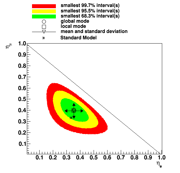
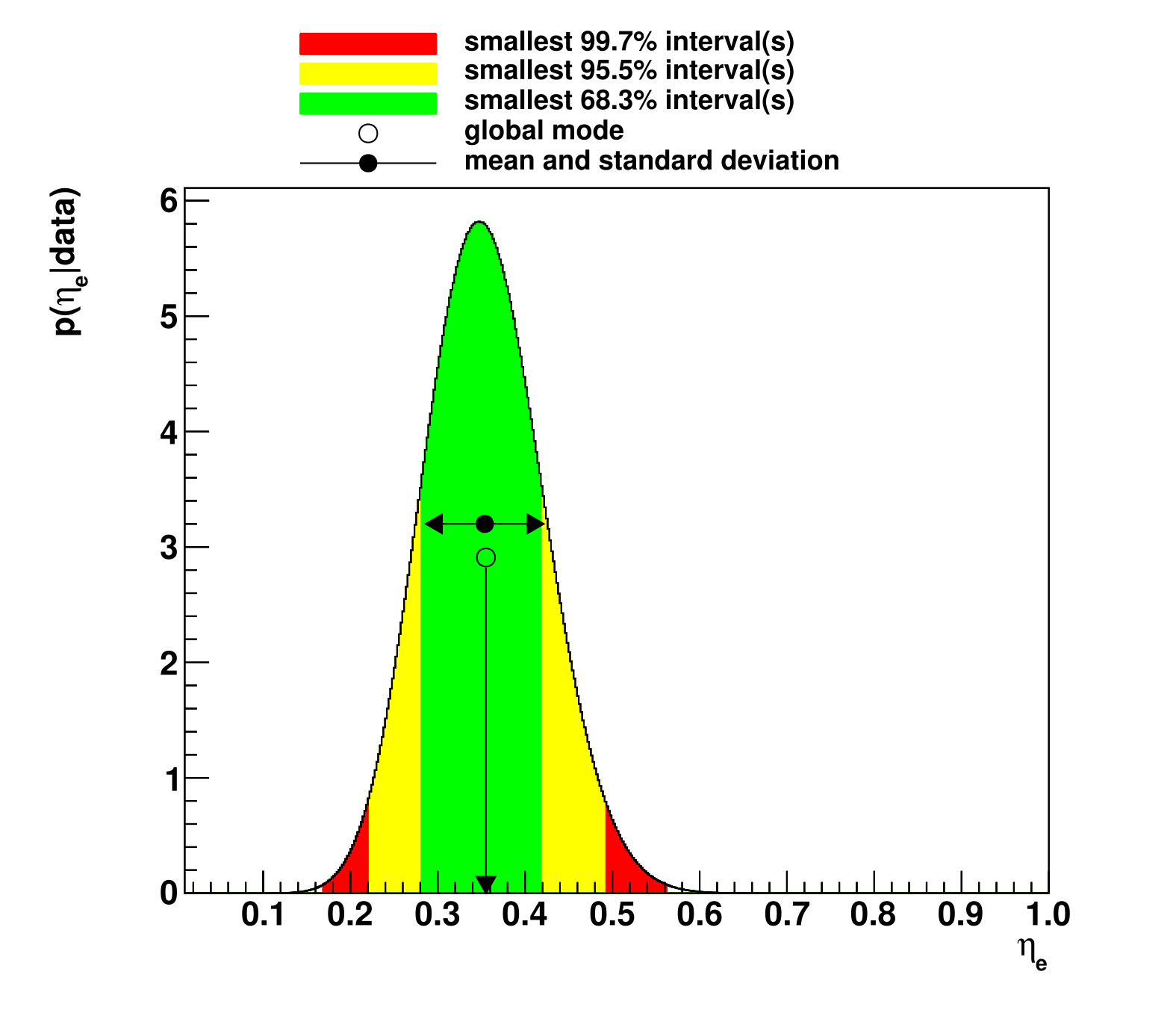
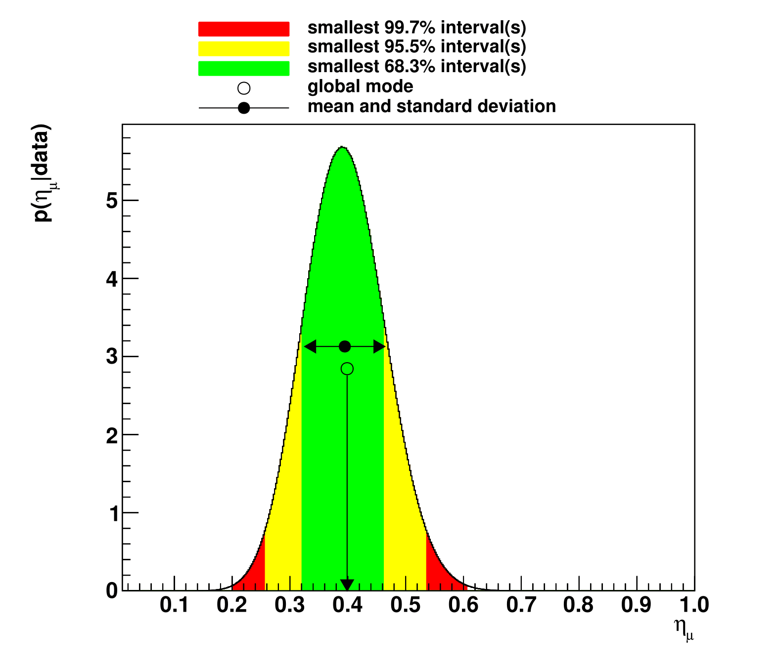
The resulting two-dimensional marginal posterior, depending on $\eta_{e}$ and $\eta_{\mu}$, is shown in Fig.1, together with the corresponding one-dimensional projections. The expectation from lepton universality, i.e., $\eta_{e}=\eta_{\mu}=1/3$, is indicated by the asterisk and consistent with the observation.

Figure 1: Contours of the smallest area containing 68.3%, 95.5% and 99.7% probability of the two-dimensional marginal posterior distribution (left), as well as the two one-dimensional posterior probability densities for $\eta_{e}$ (middle) and and $\eta_{\mu}$ (right).

3.2 Inference about $k+1$ independent Poisson sources and a single observable

Suppose that we have an experiment in which only a single count rate is measured which is known to originate from $k$ different (and possibly correlated) background sources that are known to exist, and a possible additional signal source. Taken individually, each background source is modeled as a Poisson process with parameter $b_{i}$, and the signal is an independent Poisson process with parameter $s$.

We can write the model as we did in Section 2.2 above, i.e. $P(n,\vec{Z}|s,\vec{b})$, but now we have to consider that we do not know where the individual counts come from, i.e. we have to sum over all possible configurations of $\vec{Z}$. The model thus becomes

$$P(n,\vec{Z}|s,\vec{b})\rightarrow P(n|s,\vec{b}) = \sum_{\vec{Z}}P(n,\vec{Z}|s,\vec{b})$$

$$= \text{Poi}(n|s+b)\sum_{\vec{Z}}\text{Mul}(\vec{Z}\,|n,\vec{\zeta})$$

$$= \text{Poi}(n|s+b)\,,$$

where the latter equation follows from the normalization of the multinomial distribution.

Measuring only $n$ simplifies the problem significantly, but also reduces the available information. The difference with respect to the case considered in the previous section is that the multinomial part has disappeared. In addition, the Poisson term now describes the sum of two independent sources.

One performs inference about the signal intensity $s$ by integrating the marginal posterior $p(s,b|n,\alpha,\beta)$ over $b$, where $\alpha$ and $\beta$ describe the signal prior. The objective result is the reference marginal posterior for $s$ computed in [6]

$$p(s|n)\propto e^{-s}\,f(s;n,\alpha,\beta)\,\pi(s)$$ (33)

where the polynomial

$$f(s;n,\alpha,\beta)=\sum_{m=0}^{n}\binom{\alpha+m-1}{m}\frac{s^{n-m}}{(n-m)!\,(1+\beta)^{m}}$$ (34)

behaves like $(s+\alpha/\beta)^{n}$ when both $\alpha,\beta$ are very large. Using Wolfram’s Mathematica, another representation can be found for this polynomial, in terms of the confluent hypergeometric function of the second kind $U(a,b,x)$:

$$f(s;n,\alpha,\beta)=s^{n}\,[(1+\beta)s]^{\alpha}\,U(\alpha,\alpha+n+1,(1+\beta)s)/n!$$ (35)

The reference prior $\pi(s)$ computed in [6] is an improper density, proportional to the square root of Fisher’s information computed with the marginal model:

$$|I(s)|^{1/2}=\left|\left(\frac{\beta}{1+\beta}\right)^{\!\alpha}e^{-s}\,\sum_{n=0}^{\infty}\frac{[f(s;n,\alpha,\beta)]^{2}}{f(s;n+1,\alpha,\beta)}-1\right|^{1/2}$$ (36)

Among the methods for constructing probability matching priors considered by Ventura, Cabras & Racugno [10], it comes out that only the marginal model $P(n|s)=\int\text{Poi}(n|s+b)\,\text{Ga}(b|\alpha,\beta)\,\,\mathrm{d}b$ provides a solution: no other pseudo-likelihood can be used, as it can be checked with direct calculation.

The full objective Bayesian posterior Eqn. (33) for $s$ can be computed with the help of the Bayesian Analysis Toolkit [5]. However, it is often possible to adopt a quick approximation. Despite from its complicate form (Eqn. (36)), it comes out that the reference prior admits a very simple limiting form that can be used in many practical problems [8]. It corresponds to the case of a perfectly known background, and performs very well in a wide portion of the $(\alpha,\beta)$ parameter space. As a consequence, the reference marginal posterior Eqn. (33) can be often well approximated by a single (truncated) Gamma density [8]:

$$p_{0}(s|n)=\frac{1}{C}\text{Ga}(s+\tfrac{\alpha}{\beta}|n+\tfrac{1}{2},1)$$ (37)

with normalization constant

$$\begin{split}C&=\int_{0}^{\infty}\text{Ga}(s+\tfrac{\alpha}{\beta}|n+\tfrac{1}{2},1)\,\,\mathrm{d}s=\int_{\alpha/\beta}^{\infty}\text{Ga}(x|n+\tfrac{1}{2},1)\,\,\mathrm{d}x\\ &=1-\frac{\gamma(n+\tfrac{1}{2},1)}{\Gamma(n+\tfrac{1}{2})}\end{split}$$ (38)

where the last fraction defines the regularized Gamma function, that is the cumulative distribution function corresponding to $\text{Ga}(x|n+\tfrac{1}{2},1)$, in terms of the incomplete gamma function $\gamma(n+\tfrac{1}{2},1)$ and the ordinary Gamma function.

Incidentally, we remark the similarity between the limiting reference posterior $p_{0}(s|n)$ from Eqn. (37) and the reference posterior (19) obtained when there is no background. Apart from the normalization, the former is the same as the latter with an offset $-\tfrac{\alpha}{\beta}$ in the origin. This shift might be interpreted as a form of “background subtraction”, as $\tfrac{\alpha}{\beta}$ is the prior expectation for $b$. Thus $p_{0}(s|n)$ includes the particular case of no background and generalizes the result (19) obtained with Jeffreys’ prior.

Note also that, although the multinomial part has disappeared, studies of the individual background contributions are still useful: all background sources that have a significant impact on the total background contribution $b$ — also taking into account the correlations on their uncertainty — are relevant for the inference and the conclusions drawn from the model described in Eqn. (3.2). One has also to be careful to consider any systematic effect that may have an impact on the overall background uncertainty. For example, the latter could be sensitive to a pair of strongly anti-correlated sources of background, even though their variations in opposite directions have no net effect on $b$. Hence they cannot be neglected in the analysis of systematics. In contrast those background sources, which do not contribute significantly to $b$ nor impact on its uncertainty, can be ignored in the inference about $s$.

A simple example, continued

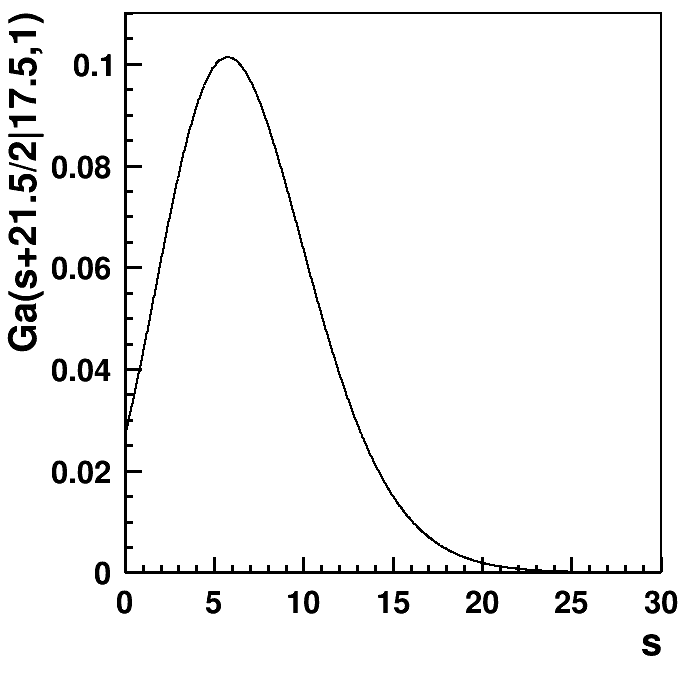
After the background radioactivity in the new lab has been estimated by making use of the results of two experiments, a potentially radioactive source is brought in, to estimate its intensity. The signal that we want to estimate is the intensity of the new source, and the measurement is performed in a laboratory in which we know already that some background radioactivity is detectable. For simplicity, the measurement is conducted in the same time interval as the previous measurements. It yields $n_{3}=17$. Using the reference prior for the signal and the posterior of the second measurement of the background as informative prior, from Eqn. (37) one gets the posterior distribution $p_{0}(s|17)\propto\text{Ga}(s+\tfrac{21.5}{2}|17.5,1)$ which is shown in Fig. 2. The posterior peaks at $s=5.75$, while the median (mean) for the signal is at 6.6 (7.0), and the central 68.3% credible interval around it (defined by the 15.85% and 84.15% posterior quantiles) is $[3.0,11.0]$. The 95% upper bound on the signal is $s<14.2$.

Figure 2: Marginal posterior of the signal intensity of the new radioactive source.

3.3 Inference about the strength of a signal distributed over several channels

In case a signal is distributed over several channels and each of these channels features a different background level, one can use the likehood defined in Eqn. 15 to infer on the signal strength. As an example, we consider the decay of a particle into three different channels. The total number of observed events is $n=62$ and they are distributed among the three channels as $n_{1}=21$, $n_{2}=29$ and $n_{3}=12$. The background contributions are assumed to be known from auxilliary measurements and their priors are modeled with Gamma densities with mean values and standard deviations of $b_{1}=10\pm 1$, $b_{2}=6\pm 1$ and $b_{3}=2\pm 0.5$. We use a Dirichlet prior for the branching ratios $s_{i}/s$ with concentration parameters 0.75, 1.5 and 0.75, respectively, resulting in expectation values of 0.25, 0.5 and 0.25 with relative uncertainties of up to about 30%. We choose a Jeffreys prior for the signal contribution.

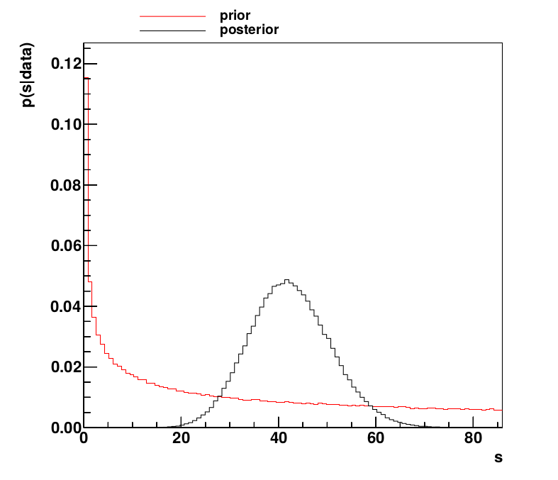
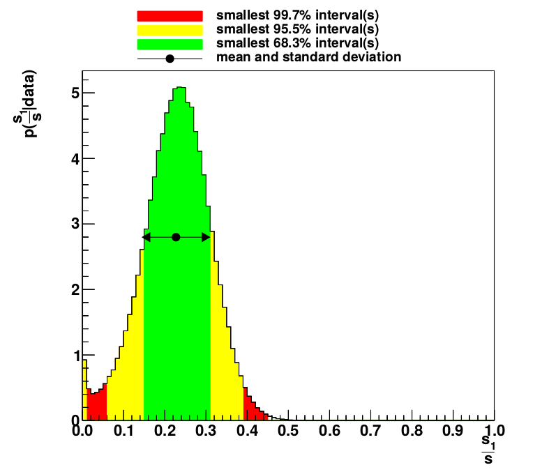
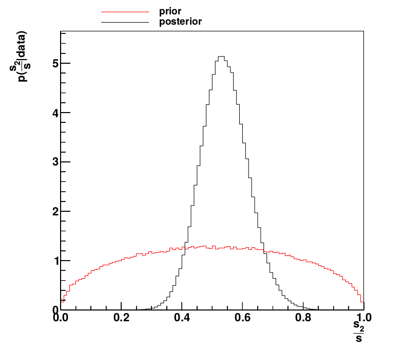
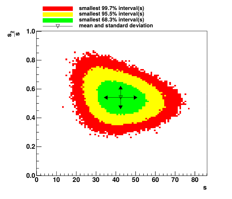
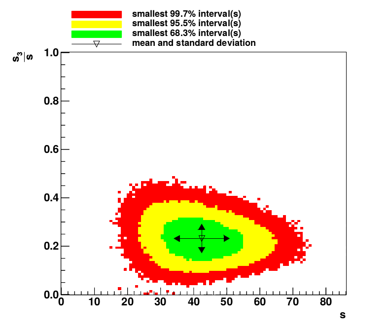
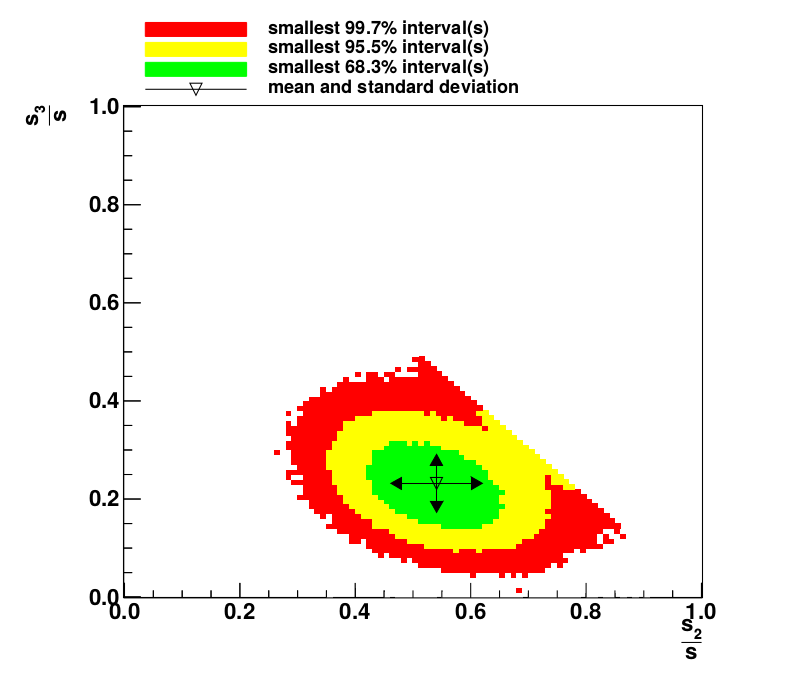
Fig. 3 shows a comparison of the prior and posterior probabilities for the signal parameter $s$ (left) and the branching ratio $s_{2}/s$ (right). Also shown is the posterior probability density for the branching ratio $s_{1}/s$ (middle). The posterior mean and standard deviation of the marginalized posterior probability of $s$ are 42.4 and 8.4, respectively. The mean value is close to the mode of the distribution, and, compared to the naive expectation of $s=n-\mathrm{E}[b]=44$, it is shifted towards smaller values due to the steeply falling prior probability. Note that the shift is small compared to the standard deviation. The mean values of the branching ratio posteriors for $s_{1}/s$ and $s_{2}/s$ are 0.54 and 0.23, respectively. The standard deviation is 0.08 in both cases, in accordance with the expectation. As expected, the inference process has a negligible impact on the posterior probability densities of the background contributions. Fig. 4 shows the smallest intervals containing 68.3%, 95.5% and 99.7% posterior probability for the two-dimensional distributions of $s_{2}/s$ vs. $s$ (left), $s_{3}/s$ vs. $s$ (middle), and $s_{3}/s$ vs. $s_{2}/s$ (right). Also indicated are the mean and standard deviations. All three distributions show weak anti-correlations. The latter distribution also shows a sharp cut-off at the physical boundary (the sum of $s_{2}/s$ and $s_{3}$ can at most be unity).

Figure 3: Comparison of the prior (red) and posterior probabilities (black) for the signal parameter $s$ (left) and the branching ratio $s_{2}/s$ (right). Also shown in the posterior probability density for the branching ratio $s_{1}/s$ (middle) including the smallest intervals containing 68.3%, 95.5% and 99.7%.

Figure 4: Smallest intervals containing 68.3%, 95.5% and 99.7% posterior probability for the two-dimensional distributions of $s_{2}/s$ vs. $s$ (left), $s_{3}/s$ vs. $s$ (middle), and $s_{3}/s$ vs. $s_{2}/s$ (right). Also indicated are the mean and standard deviations.

4 Summary

In this paper, we have derived a statistical model for counting experiments in which the sources contributing to the resulting count rate are potentially correlated. Using Bayes’ theorem and assuming non-informative and informative priors on signal and background contributions respectively, we have shown that the marginal posterior probability for the signal contribution can be expressed in closed form. Simple use cases in the field of experimental physics have been presented.

5 Useful properties of the multinomial distribution

We recall here a few properties of the multinomial distribution that are important when considering practical problems, in particular its behavior under re-binning and partitioning.

The first one is about re-binning: merging random variables distributed according to multinomial distributions again gives a multinomial distribution. If $\vec{X}\sim\text{Mul}(n,\vec{\eta})$ with $\vec{\eta}\equiv(\eta_{1},\eta_{2},\ldots,\eta_{k})$, then $\vec{X}^{*}\equiv(X_{1}+X_{2},X_{3},\ldots,X_{k})\sim\text{Mul}(n,\vec{\eta}^{*})$ where $\eta_{1}^{*}\equiv\eta_{1}+\eta_{2}=(\lambda_{1}+\lambda_{2})/\lambda$ and $\eta_{j}^{*}\equiv\eta_{j+1}$ for $j=2,3,\ldots,k-1$. One may obtain a binomial problem by sequentially merging $k-2$ bins.

The second property is important if we know the total number of counts $n^{\prime}$ in a subset of the bins: the conditional distribution given that $X_{1}+X_{2}=n^{\prime}$ and $X_{3}+\ldots+X_{k}=n-n^{\prime}$ is a product of two independent multinomial pieces:

$$\begin{split}(X_{1},X_{2})&\sim\text{Mul}(n^{\prime},\frac{\eta_{1}}{\eta_{1}+\eta_{2}},\frac{\eta_{2}}{\eta_{1}+\eta_{2}})\\ (X_{3},\ldots,X_{k})&\sim\text{Mul}(n-n^{\prime},\frac{\eta_{3}}{\sum_{J=3}^{k}\eta_{j}},\ldots,\frac{\eta_{k}}{\sum_{J=3}^{k}\eta_{j}})\end{split}$$ (39)

For example, this property tells us how to treat two histograms at the same time.

Conversely, the third property is that the joint distribution of two independent multinomial random vectors has a multinomial kernal. To see this, one starts from

$$\begin{split}\vec{X}&\sim\text{Mul}(\vec{X}\,|n,\vec{\eta})\equiv\frac{n!}{X_{1}!\,X_{2}!\,\cdots X_{k}!}\,\eta_{1}^{X_{1}}\,\eta_{2}^{X_{2}}\,\cdots\,\eta_{k}^{X_{k}}\;,\;\sum_{j=1}^{k}\eta_{j}=1\;,\;\sum_{j=1}^{k}X_{j}=n\\ \vec{Y}&\sim\text{Mul}(\vec{Y}\,|n^{\prime},\vec{\zeta})\equiv\frac{n^{\prime}!}{Y_{1}!\,Y_{2}!\,\cdots Y_{m}!}\,\zeta_{1}^{Y_{1}}\,\zeta_{2}^{Y_{2}}\,\cdots\,\zeta_{m}^{Y_{m}}\;,\;\sum_{j=1}^{m}\zeta_{j}=1\;,\;\sum_{j=1}^{m}Y_{j}=n^{\prime}\end{split}$$

and writes their joint distribution as

$$\begin{split}\vec{X},\vec{Y}&\sim\text{Mul}(\vec{X}\,|n,\vec{\eta})\,\text{Mul}(\vec{Y}\,|n^{\prime},\vec{\zeta})\\ &=\frac{n!}{X_{1}!\,X_{2}!\,\cdots X_{k}!}\,\frac{n^{\prime}!}{Y_{1}!\,Y_{2}!\,\cdots Y_{m}!}\,\eta_{1}^{X_{1}}\,\eta_{2}^{X_{2}}\,\cdots\,\eta_{k}^{X_{k}}\,\zeta_{1}^{Y_{1}}\,\zeta_{2}^{Y_{2}}\,\cdots\,\zeta_{m}^{Y_{m}}\end{split}$$ (40)

Defining

$$\vec{Z}\equiv(\vec{X},\vec{Y})$$ (41)

such that $Z_{i}=X_{i}$ for $i=1,\ldots,k$ and $Z_{i}=Y_{i-k}$ for $i=k+1,\ldots,k+m$, one has

$$\sum_{j=1}^{k+m}Z_{j}=n+n^{\prime}$$

Furthermore, defining

$$\vec{\xi}\equiv\frac{1}{2}(\vec{\eta},\vec{\zeta})$$ (42)

one also has

$$\sum_{j=1}^{k+m}\xi_{j}=1$$

such that Eqn. (40) may be rewritten as

$$\begin{split}\vec{Z}&\sim\frac{2^{n+n^{\prime}}\,n!\,n^{\prime}!}{Z_{1}!\,Z_{2}!\,\cdots Z_{k+m}!}\,\,\xi_{1}^{Z_{1}}\,\xi_{2}^{Z_{2}}\,\cdots\,\xi_{k+m}^{Z_{k+m}}\end{split}$$ (43)

where we used $\prod_{j=1}^{k+m}2^{Z_{j}}=2^{\sum_{j=1}^{k+m}Z_{j}}=2^{n+n^{\prime}}$.

This looks like a multinomial with $k+m-1$ degrees of freedom. However, we started from two multinomials with $k-1$ and $m-1$ degrees of freedom, hence must obtain a distribution with $k+m-2$ free parameters. Eqn. (43) gives the probability distribution conditional to $n$ and $n^{\prime}$. If, however, only the total number of counts $n_{\text{tot}}=n+n^{\prime}$ is known, then one must sum Eqn. (43) over all possible pairs of $n$ and $n^{\prime}$ which result in a total count of $n_{\text{tot}}$. This reduce by one the number of independent variables.

References

- Berger & Bernardo [1992] J.O. Berger & J.M. Bernardo, Ordered Group Reference Priors with Application to the Multinomial Problem, Biometrika 79 (1992) 25-37.
- Berger, Bernardo & Sun [2013] J.O. Berger, J.M. Bernardo, D. Sun, Objective priors for discrete parameter spaces, J. Amer. Statist. Assoc. 107 (2012) 636.
- Berger, Bernardo & Sun [2013] J.O. Berger, J.M. Bernardo, D. Sun, Overall Objective Priors, conference on “Recent advances in statistical inference: theory and case studies”, University of Padova, 21–23 Mar 2013.
- [4] J.M. Bernardo, “Reference analysis”, Handbook of Statistics 25 (D.K. Dey and C.R. Rao eds.). Amsterdam: Elsevier (2005) 17–90.
- [5] A. Caldwell, D. Kollar, K. Kröninger, BAT - The Bayesian Analysis Toolkit, Computer Physics Communications 180 (2009) 2197-2209 10.1016/j.cpc.2009.06.026, arXiv: 0808.2552.
- Casadei [2012] D. Casadei, Reference analysis of the signal + background model in counting experiments, JINST 7 (2012) P01012, 10.1088/1748-0221/7/01/P01012, arXiv: 1108.4270.
- Casadei [2012] D. Casadei, Estimating the selection efficiency, JINST 7 (2012) P08021, 10.1088/1748-0221/7/08/P08021, arXiv: 0908.0130.
- Casadei [2012] D. Casadei, Reference analysis of the signal + background model in counting experiments II. Approximate reference prior, JINST9 (2014) T10006, 10.1088/1748-0221/9/10/T10006, arXiv: 1407.5893.
- [9] K. A. Olive et al. [Particle Data Group Collaboration], Review of Particle Physics, Chin. Phys. C 38 (2014) 090001, 10.1088/1674-1137/38/9/090001.
- Ventura, Cabras & Racugno [2009] L. Ventura, S. Cabras, W. Racugno, Prior distributions from pseudo-likelihoods in the presence of nuisance paramenters, J. Amer. Statist. Assoc. 104 (2009) 768.