Diagnostics of Ellerman Bombs with High-resolution Spectral Data

Abstract

Ellerman bombs (EBs) are tiny brightenings often observed near sunspots. The most impressive characteristic of the EB spectra is the two emission bumps in both wings of the H$\alpha$ and Ca II 8542 Å lines. High-resolution spectral data of three small EBs were obtained on 2013 June 6 with the largest solar telescope, the 1.6 meter New Solar Telescope (NST), at the Big Bear Solar Observatory. The characteristics of these EBs are analyzed. The sizes of the EBs are in the range of 0.3-0.8 and their durations are only 3–5 minutes. Our semi-empirical atmospheric models indicate that the heating occurs around the temperature minimum region with a temperature increase of 2700–3000 K, which is surprisingly higher than previously thought. The radiative and kinetic energies are estimated to be as high as 5$\times$10²⁵–3.0$\times$10²⁶ ergs despite the small size of these EBs. Observations of the magnetic field show that the EBs appeared just in a parasitic region with mixed polarities and accompanied by mass motions. Nonlinear force-free field extrapolation reveals that the three EBs are connected with a series of magnetic field lines associated with bald patches, which strongly implies that these EBs should be produced by magnetic reconnection in the solar lower atmosphere. According to the lightcurves and the estimated magnetic reconnection rate, we propose that there is a three phase process in EBs: pre-heating, flaring and cooling phases.

1 Introduction

Ellerman bombs (EBs: Ellerman [1917]) are small short-lived brightening events. Thier most obvious feature is the excess emission in the wings of chromospheric lines (Koval & Severny [1970]; Bruzek [1972]). Since the 1970s, EBs have been widely studied. Recently, using imaging data with high spatiotemporal resolutions, it was found that the lifetime of some EBs can be as short as 2–3 minutes, and their size can be smaller than 1 (Vissers et al. [2012]; Nelson et al. [2013]). It was also shown that generally EBs have elongated structures (Matsumoto et al. [2008]; Watanabe et al. [2008, 2011]; Hashmoto et al. [2010]; Vissers et al. [2013]). The temperature increase of EBs was generally thought to be around 600–1500 K (Kitai  [1983]; Fang et al. [2006]; Hong et al. [2014]). Georgoulis et al.( [2002]) used high-resolution chromospheric H$\alpha$ filtergrams and found that the temperature enhancement of EBs is $\sim 2\times 10^{3}$ K. Furthermore, using high-resolution H$\alpha$ images, Berlicki et al.( [2010]) found that the temperature increase could be as high as 3000 K. Mass motion is another feature associated with EBs. It was found that some EBs have an upward motion with a velocity of several km s^-1 (Kurokawa et al. [1982]; Dara et al. [1997]; Yang et al  [2013]). Some observations of EBs at the solar limb also found up-flows (Kurokawa et al. [1982]; Nelson et al.  [2015]). Only a few observations indicated that there are also downward photospheric motions (Georgoulis et al. [2002]; Yang et al. [2013]). Matsumoto et al.( [2008]) observed bi-directional flows associated with EBs as evidence of magnetic reconnection. It was estimated that the energy of EBs is in the range of 10²⁵ – 10²⁷ ergs (Teske [1971]; Bruzek [1972]; Hénoux et al. [1998]; Fang et al. [2006]). Georgoulis et al.( [2002]) obtained a higher energy of EBs to be 3$\times$10²⁸ ergs. However, using a similar value of the net radiative loss rate and taking the height of a EB to be 100 km, Nelson et al. ( [2013]) estimated the EB energies being in the range of $2\times 10^{22}$ – 4 $\times 10^{25}$ ergs, which is three to four orders of magnitude lower than that in Georgoulis et al.( [2002]). To elucidate the physical mechanism of EBs, spectral data with high spatial and temporal resolutions are imperative. However, up to now, only a few such observations are available.

To understand the driving mechanism of EBs, it is necessary to study the relationship between EBs and magnetic features. It was found that most EBs are located near magnetic inversion lines (Dara et al. [1997]; Qiu et al. [2000]). Georgoulis et al.( [2002]) found that EBs may occur on separatrix or quasi-separatrix layers. Vissers et al.( [2013]) found that EBs occur at sites of magnetic flux cancellation between small bipolar patches. Many authors proposed that magnetic reconnection in the photosphere or chromosphere could be a mechanism for EBs (Hénoux et al.[1998]; Ding et al.  [1998]; Georgoulis et al. [2002]; Fang et al.  [2006]; Pariat et al. [2007]; Isobe et al. [2007]; Matsumoto et al. [2008]; Watanabe et al. [2008];  [2011]; Archontis & Hood  [2009]; Yang et al. [2013]; Nelson et al.  [2013]). Based on magnetic extrapolation, Pariat et al.( [2004]) proposed that EBs could be produced by magnetic reconnection at bald patches or along the separatrices in the low chromosphere. We have performed two-dimensional numerical magnetohydrodynamic simulations on the magnetic reconnection in the solar lower atmosphere (Chen et al.  [2001]; Jiang et al. [2010]; Xu et al. [2011]). Our results indicated that magnetic reconnection in the lower solar atmosphere can explain the temperature enhancement and lifetime of EBs, and the main reason is that ionization processes in the upper chromosphere consumes a large part of the released magnetic energy, resulting in little heating in this layer.

In this paper, we use high-resolution spectral data of H$\alpha$ and Ca II 8542 Å lines, which were obtained on 2013 June 6 with the largest aperture solar telescope in the world, the 1.6 meter off-axis New Solar Telescope (NST) (Goode et al.  [2012]; Cao et al. [2010]) at the Big Bear Solar Observatory (BBSO). The characteristics of three well-observed small EBs are analyzed. The data acquisition with the NST is described in §2. The characteristics of the EBs are analyzed in §3, including the two-dimensional (2D) velocity distribution, their relationship with the magnetic field, and the intensity evolution of the EBs. With semi-empirical atmospheric modeling, the energetics and magnetic reconnection rates of the EBs are estimated in §4. General discussions and conclusions are given in §5.

2 High-resolution spectral data of three small EBs

On 2013 June 6 a part of the active region NOAA 11765 (N09E10) was observed from 16:50 UT to 19:00 UT (there are gaps in the collection of data) by the Fast Imaging Solar Spectrograph (FISS)(Chae et al. [2013]) of BBSO/NST. FISS is a dual-band echelle spectrograph. It has two cameras, one for H$\alpha$ band with effective 512$\times$256 pixels, one for Ca II band with effective 502$\times$250 pixels. With fast scanning of the slit across the field of view, high-resolution 2D imaging spectra in H$\alpha$ and Ca II 8542 Å bands were obtained simultaneously. The dispersions for H$\alpha$ and Ca II 8542 Å lines are 0.019 Å and 0.026 Å per pixel, respectively. The active region was scanned repeatedly 160 times. Each scan covered 150 steps separated by 0.16 in space and lasted 28–30 s. The spatial sampling along the slit was 0.16 per pixel. The field of view of each scan is about 40 $\times$ 25 . The exposure times were 30 ms and 60 ms for H$\alpha$ and Ca II 8542 Å lines, respectively. Seeing condition was better than 1.0. Using the newly developed adaptive optics (AO) systems with 308 actuators, the diffraction limit was achieved.

3 Main characteristics of the small EBs

By carefully checking the high-resolution spectra, we found three well-observed small EBs during the observations. The criteria for detecting EBs is the existence of excess emissions at the far wings of the H$\alpha$ lines. Table 1 lists some characteristics of the three EBs, numbered No.1–No.3, including the time when the EB intensity attains the maximum, $\Delta I$, duration $D$, size, accompanied downward velocity, and $\Delta T$. Here $\Delta I$ is the intensity difference between the EB H$\alpha$ peak (at $\sim-1$ Å) and the nearby background, with a unit of 10⁶ erg s^-1 cm^-2 sr^-1 Å^-1. Note that the nearby background is a pre-heated area, not the quiet-Sun further away, which has a lower intensity at the center of H$\alpha$ lines as shown in Figure 1. The durations ($D$) of the EBs are estimated by the scanning time during which the EB emission in the far wing of the H$\alpha$ line can still be identified. The sizes of EBs were determined by the full-width at half-maximum (FWHM) of the lightcurves along the successive scan ($x$) and along the slit ($y$) directions, when the EBs can still be identified. A 2D Doppler velocity distribution was recovered from spatially resolved H$\alpha$ line profiles with the centroid method. $\Delta T$ is the peak temperature difference between that in our EB semi-empirical models (see §4) and that of the quiet-Sun model.

Figure 1: The left column shows the observed H$\alpha$ and Ca II 8542 Å line profiles of the EB No. 2 (solid lines), the line profiles of the nearby background (N; dotted lines), and those of the quiet-Sun (Q; dashed lines). The excess intensities $\Delta I$, i.e., the EB intensity with the nearby background being subtracted (EB-N), are shown in the two panels on the right column.

Table 1: Characteristics of the EBs

No.	Time	$\Delta I$	Duration	Size ($x\times y$)	Downward $v_{\parallel}$	$\Delta T$
	(UT)	(106 erg s-1 cm-2 sr-1 Å-1 )	(s)	(arcsec)	(km s-1)	(K)
1	17:03:04	$\geq$0.30	300	0.306$\times$ 0.310	4	2740
2	17:09:55	$\geq$0.35	220	0.464$\times$ 0.368	5	2810
3	17:22:03	$\geq$0.30	223	0.557$\times$ 0.765	5	2940

Table 1 shows that the sizes of the EBs are in the range of 0.3-0.8 with elongated structures, though the No.1 EB has a more or less round structure. Moreover, all the EBs are accompanied by downward flows.

3.1 H$\alpha$ and Ca II 8542 Å line profiles of the EBs

As an example, the H$\alpha$ and Ca II 8542 Å line profiles of the EB No. 2 are shown as solid lines in the top-left panel and the bottom-left panel of Figure 1, respectively. For comparison, the dotted lines are the counterparts of the nearby (N) background and the dashed lines indicate the line profiles of the quiet-Sun regions (Q). The line profiles of the EB after subtracting those of the nearby background, EB-N, are also shown in the top-right and bottom-right panels. It can be seen that the EB-N profiles exhibit obvious excess emissions at the blue and red wings, which is a typical characteristic of EBs. It implies that the heating is significant in the solar lower atmosphere. All these will be clearly seen in our computed semi-empirical atmospheric models shown later in §4. It should be emphasized that comparing to the quiet-Sun line profiles, there is an intensity enhancement at the EB H$\alpha$ line center. It implies that a heating still exists in the corresponding upper chromosphere. Note that the intensities at the blue and red wings are asymmetric, and sometimes the blue wing is even stronger than the red wing. The asymmetry might be produced by the dynamical processes in the EBs.

3.2 2D magnetic and velocity maps around the EBs

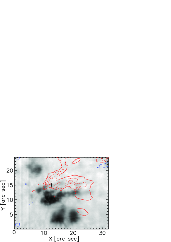
Figure 2: Velocity distribution (contours) around 17:09:55 UT superposed on the H$\alpha$ blue wing ($-0.99$ Å  from the line center) image (gray scale). The cross sign pinpoints the EB No. 2. The contour levels of the Doppler velocity are -2, 3 (solid lines), 8 (dashed lines) and 12 (dotted lines) km s^-1. The blue and red lines correspond to upward and downward velocities, respectively. Several vertical lines visible are the remains after the instrumentation artifact elimination.

Figure 2 displays the location of the EB No. 2 on the 2D FISS H$\alpha$ raster images taken at the far wing. The cross sign pinpoints the EB. The contours show the velocity distribution around 17:09:55 UT with the Doppler velocity levels of -2, 3, 8, 12 km s^-1. Figure 2 shows that the EB has a co-spatial relationship with the downward mass motion measured in the H$\alpha$ profile.

To derive the topology of magnetic field of the EBs, we make a nonlinear force-free field (NLFF) extrapolation with an optimization method (Wheatland et al. [2000]; Wiegelmann et al. [2004]). The vector magnetogram is observed by the Helioseismic and Magnetic Imager (HMI; Scherrer et al. [2012]; Schou et al [2012]) on board the Solar Dynamics Observatory (SDO). First, we remove the 180^∘ ambiguity of the transverse components of the vector magnetogram using the minimum energy method (Metcalf et al. [2006]; Leka et al. [2009]). Then, we correct the projection effect using the method mentioned in Gary & Hagyard( [1990]). The vertical component of the projection corrected magnetic field is shown in Figure 3. Next, a preprocessing technique (Wiegelmann et al.  [2006]) is applied to the vector magnetic field in the field of view as shown in Figure 3 to remove the net magnetic force and torque. Finally, we derive the NLFF that is shown in Figure 4. It shows that EB No.2 is co-spatial with a bipole, and EBs No.1 and No.3 are connected to the bipole with magnetic field lines as shown in the right panel of Figure 4. We can see that the three EBs are located in the region with parasitic magnetic elements showing mixed polarities, and are connected with a series of magnetic field lines associated with bald patches, where the magnetic field lines are tangential to the photosphere and concave up.

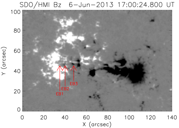
Figure 3: Vertical component of the projection-corrected magnetic field. The arrows indicate the positions of the three EBs.

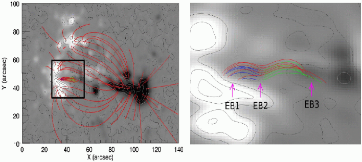
Figure 4: Nonlinear force-free field extrapolated around the EBs. The black box in the left panel indicates the field of view of the right panel. Since the perspective of the right panel is different from that of the left one, the figure on the bottom is stretched. The left panel shows a large field of view, where the extrapolation is performed. The right panel focuses on a small field of view around the EBs.

3.3 Intensity evolution of the EBs

High spatial-resolution and high-cadence observations allow us to obtain the intensity evolution at the H$\alpha$ far-wing ($\sim-1$ Å) of the three EBs as shown in Figure 5. Two dashed lines indicate the time when the excess emission in the wing of H$\alpha$ lines appears and disappears, respectively. The durations of the EBs listed in Table 2 are just taken as the time intervals between the appearance and the disappearance of the excess emission of the EBs. According to the property of the lightcurves, which are made from the single pixel where the EB brightening attends the maximum, we can distinguish three phases of the EB evolution: a pre-heating phase, when the intensity increased slowly but continuously, and the excess emission at the far wing of the H$\alpha$ lines is absent or very weak; a flaring phase, in which the intensity increased quickly and the excess emission at the H$\alpha$ line wings attained the maximum at the peak time; and then a cooling phase when the intensity decayed rapidly. The estimation of the magnetic reconnection rate (see §4) indicates that the flaring phase is produced by fast magnetic reconnection. It seems that the pre-heating phase corresponds to a slow magnetic reconnection process, which produces micro-turbulence. When it reaches a certain critical state, fast magnetic reconnection commences. The cooling phase is short. Potentially, this is due to the strong radiative loss in the solar lower atmosphere, where the EBs occur.

Figure 5: Lightcurves of the three EBs (in counts) at the far wings ($\sim$ -1 Å) of their H$\alpha$ line profiles. From top to bottom: the start time is 16:58:59 UT, 17:00:21 UT and 17:16:55 UT for EBs No. 1, No. 2, and No. 3, respectively. Two dashed lines mark the moments when the excess emission at the H$\alpha$ far wing appears and disappears, respectively. The intensities plotted in this Figure are for one pixel where the EBs have the peak intensities.

4 Semi-empirical modelling of the small EBs

4.1 Non-LTE computation of the semi-empirical models

The semi-empirical atmospheric models of EBs can be computed by using the H$\alpha$ and Ca II 8542 Å line profiles. We follow the non-local thermal equilibrium (non-LTE) calculation method as described in the paper of Fang et al.( [2006]). We solve the statistical equilibrium equation, the transfer equation, the hydrostatic equilibrium, and the particle conservation equations iteratively. The relative difference of the mean intensity between the last two iterations is less than 10^-7 and 10^-8 for hydrogen and calcium atoms, respectively.

Figure 6: Comparison between the observed (dotted lines) and non-LTE computed (solid lines) H$\alpha$ and Ca II 8542 Å line profiles for the EB No. 2. We can see the widening of the H$\alpha$ lines and the red shifting of both observed lines. These properties are discussed in the text.

Figure 7: Temperature distributions in the semi-empirical model of the EB No. 2 (solid line), compared to that of the plage model (dashed-dotted line) given by Fang et al.( [2001]), and that of the quiet-Sun model (i.e., the VALC model, dashed line) given by Vernazza et al.( [1981]).

As an example, Figure 6 gives both the observed and computed H$\alpha$ and Ca II 8542 Å line profiles for the EB No. 2. It can be seen that the modeled profiles can well match the observed ones, except two aspects: (1) the computed H$\alpha$ line profile is narrower than the observed one. This is probably due to the existence of turbulence in the EB heating region, which might be caused during the magnetic reconnection and we did not include in our computation; (2) The observed line profiles show red shifts compared to the computed ones. This clearly indicates that there is a downward motion also contributing to the H$\alpha$ profile at this spatial position. We did not take this effect into account in our modeling. Figure 7 gives the semi-empirical atmospheric model of the EB No. 2. For comparison, we also plot the temperature distributions in the semi-empirical model for plages (denoted by “Plage”) as derived by Fang et al.( [2001]) and for the quiet-Sun model (denoted by “VALC”) in Vernazza et al.( [1981]). It can be seen there is a temperature increase, albeit weak, in the upper chromosphere at the site of the EB, which is necessary to produce the intensity increase of the EB at the center of the chromospheric lines compared to the quiet-Sun one (see Figure 1 in §3). The most distinct feature in the semi-empirical model is an obvious heating around the temperature minimum region and in the upper photosphere, which is responsible for the excess emission at the far wings of the EB spectra. The maximum temperature enhancements for the three EBs are in the range of 2700–3000 K (see Table 1), which is consistent with the high-resolution observation by Berlicki et al.( [2010]), but much higher than other previous values (e.g., Fang et al. [2006]). The difference maybe comes from the fact that the previous observations with a lower spatial resolution blended the EB intensity and the quiet-Sun one, and resulted in weaker intensity than that in the high-resolution observations. It is noted, however, that by use of the BBSO data, Hong et al.( [2014]) found a lower temperature in EBs. This is because they used an averaged (across an area over 2) intensity line profile.

4.2 Energy estimation of the EBs

We use the method given in Fang et al.( [2006]) to estimate the energy of EBs. It is hypothesized that the main heating regions of EBs are in the lower chromosphere and the upper photosphere, so we can use the following equation to estimate the radiative energy $E_{r}$ of EBs:

$$E_{r}={D\over 2}A_{EB}\int_{h_{1}}^{h_{2}}{R_{r}}\,d{h}\,\,,$$ (1)

where the heating duration is assumed to be half of the EB lifetime $D$. $A_{EB}$ is the area of the EB, which was determined by the EB size ($x\times y$) listed in Table 1. In Eq. (1), $h_{1}$ and $h_{2}$ are the lower and the upper heights of the heated region, including the heating in the chromosphere, $R_{r}$ the Non-LTE radiative losses in unit of erg cm^-3 s^-1. Gan et al.( [1990]) provided a semi-empirical formula for estimating $R_{r}$, but here we use an improved empirical formula given by Jiang et al.( [2010]) and shown as follows. This formula is more suitable for the small-scale activities.

$$R_{r}=n_{H}n_{e}({\alpha_{1}(h)}+{\alpha_{2}(h)})f(T)\,,$$ (2)

where

$log~{}{\alpha_{1}(h)}=1.745\times 10^{-3}h-4.739$ ,

$\alpha_{2}(h)=8.0\times 10^{-2}e^{-3.701\times 10^{-2}h}$ ,

$f(T)=4.533\times 10^{-23}{(T/10^{4})}^{2.874}$ ,

where $h$ is the height in kilometers. To estimate the net radiative energy $\Delta E$ of the EBs, we have to subtract the radiative energy of the quiet-Sun ($E_{Q}$) from that of EBs ($E_{r}$):

$$\Delta E=E_{r}-E_{Q}\,\,.$$ (3)

$E_{Q}$ can be estimated by ${D\over 2}A_{EB}\int{R_{Q}}d{h}$, where $\int{R_{Q}}dh$ is the radiative losses in the quiet-Sun atmosphere. According to the result of Vernazza et al.( [1981]), we take $\int{R_{Q}}d$h = 4.6$\times 10^{6}$ erg cm^-2 s^-1.

The lower limit of the kinetic energy can be estimated by use of the line-of-sight velocity near the EBs as

$$E_{v}={1\over 2}\times 1.4m_{H}v_{\parallel}^{2}fA_{EB}\int_{h_{3}}^{h_{4}}n_{H}d{h}\,\,,$$ (4)

where $n_{H}$ is the hydrogen density, $f$ the fraction of the mass involved in the motion. We assume $f=0.1$ as in our previous paper (Fang et al.  [2006]). The coefficient 1.4 is used for including the contribution from helium. $h_{3}$ and $h_{4}$ denote the lower and the upper heights of the EB main heating region (corresponding to the temperature bump region, see Figure 7), respectively. Actually, we take $h_{3}$ = $h_{1}$, which are obtained from our semi-empirical models of the EBs. Considering the rapid decrease of the hydrogen density with height, we neglect the contribution from the higher layers.

Using Eqs. (3) and (4), the energies of the EBs can be estimated, which are listed in Table 2. It can be seen that the total energy is about 5$\times$10²⁵–3.0$\times$10²⁶ ergs, which is in the lower limit range given by previous authors (e.g. Georgoulis et al. [2002]; Fang et al. [2006]). Considering the fact that these are three small EBs, it is reasonable. In our cases, the radiative and kinetic energies of the EBs are comparable.

Table 2: Energies and reconnection rates for the three EBs

EB	h1, h3	h2	h4	$\Delta E$	$E_{v}$	$B$	$R$
	(km)	(km)	(km)	(erg)	(erg)	(G)
No. 1	363	1926	760	3.12$\times 10^{25}$	1.57$\times 10^{25}$	200–300	0.12–0.036
No. 2	337	2044	847	6.11$\times 10^{25}$	7.14$\times 10^{25}$	200–300	0.13–0.040
No. 3	395	2386	804	2.02$\times 10^{26}$	7.05$\times 10^{25}$	250–350	0.19–0.071

4.3 Estimation of the magnetic reconnection rate

Assuming that the thermal and kinetic energies of EBs come from the dissipation of magnetic field during magnetic reconnection, we can estimate the magnetic reconnection rate. Suppose that the heating region of the EBs is the magnetic energy dissipating region, the magnetic energy coming into the region per second is

$$E_{in}={{V_{in}dlB^{2}}\over{\mu}}\,\,,$$ (5)

where $d$ is the heated atmospheric height of the EBs and $l$ is the averaged apparent size of the EBs. We take $d=h4-h3$ and $l=(x+y)/2$. $V_{in}$ is the inflow velocity, $B$ the magnetic field taken from the HMI observation, $\mu$ the magnetic permeability. If we take $E_{in}D=\Delta E+E_{v}$, we have

$$V_{in}={{\mu(\Delta E+E_{v})}\over{dlDB^{2}}}\,\,.$$ (6)

The Alfvén velocity $V_{A}=B/{\sqrt{\mu\rho}}$ and the density $\rho$ can be obtained from our semi-empirical models. So we can obtain the averaged reconnection rate, $R=V_{in}/V_{A}$, as follows:

$$R={{\mu^{3/2}\rho^{1/2}(\Delta E+E_{v})}\over{ldDB^{3}}}\,.$$ (7)

The magnetic field strength can be obtained from the photospheric magnetograms. The estimates of the reconnection rate $R$ for the three EBs are listed in Table 2. It can be seen that $R$ is in the range of 0.04–0.19, varying in different EBs and depending on the magnetic field strength, but well in the regime of fast magnetic reconnection (e.g., Priest & Forbes [2000]). It implies that the magnetic reconnection responsible for the EBs is Petschek-like fast reconnection (Petschek [1964]).

5 Discussions and Conclusions

By using the FISS data of the 1.6 meter BBSO/NST telescope, we obtained high-resolution H$\alpha$ and Ca II 8542 Å spectra of three well-observed small EBs. The high spatial resolution data allow us to study the individual EBs without much mixing with the surrounding region. The high temporal resolution data make it possible to study the evolution of the EBs in detail, so as to well clarify the different phases of the EBs.

It is shown that all the EBs are located near the parasitic areas in the longitudinal magnetograms and are co-spatial to mass motions of several km s^-1. Our NLFF extrapolation clearly shows that the EBs appear at the bald patches and the separatrices of the magnetic field, which confirms the schematic model of Pariat et al.( [2004]). Checking the lightcurves of the EBs, the evolution of the EBs can be divided into three phases: the pre-heating, flaring, and cooling phases. The estimation of the magnetic reconnection rate of the EBs indicates the occurrence of fast reconnection during the flaring phase of the EBs. These facts imply that the EBs are caused by Petscheck-type magnetic reconnection (e.g., Hénoux et al. [1998]; Ding et al. [1998]), with a rate similar to solar flares albeit with much smaller sizes. However, compared to solar flares, the cooling phase of the EBs is much shorter. It can be understood since in the solar lower atmosphere where EBs occur, the radiative losses are much stronger than that in the solar corona. Another reason is that part of the EB energy goes to heat the upper chromosphere, so the cooling of the EBs should be quicker.

Using the Non-LTE theory, we computed the thermal semi-empirical models for the three small EBs. Our results indicate that the required extra temperature enhancement in the lower atmosphere is 2700–3000 K when compared with the quiet-Sun model, as shown in Figure 7. It can account for the excess emission at the far wings of the chromospheric lines, which is the main spectral feature of EBs. The temperature enhancement in our models is larger than previous values given by some authors with lower resolution observations. Such a result is not surprising. In fact, with high spatial resolution observations, temperature increases more than 2000 K have been reported (e.g., Georgoulis et al.  [2002]; Berlicki et al. [2010]). It is probably that the temperature enhancement in many of the previous works, i.e., $\sim$1000 K, was underestimated, or some of the events are not real EBs (Rutten et al. [2013]). Another interesting thing is that compared to the plage atmospheric model, there is also a temperature enhancement in the EB upper chromosphere. It can be caused by jets or some kind of waves which are produced during the magnetic reconnection process. Actually, in our previous numerical simulations (Jiang et al. [2010]; Xu et al. [2011]), the temperature enhancement does appear in the upper chromosphere.

The semi-empirical models and the measured line-of-sight velocities near the EBs are used to estimate both the radiative and kinetic energies. Our results indicate that the total energy of these three small EBs is about $5\times 10^{25}$–3.0$\times 10^{26}$ ergs .

Based on the analysis of the three small EBs, we draw the conclusions as follows:

1. The thermal semi-empirical atmospheric models for the three small EBs clearly show the heating bump around the temperature minimum region. The temperature enhancement is about 2700–3000 K, much higher than the values obtained previously with lower-resolution spectral data.

2. All EBs are located near the parasitic magnetic areas in the longitudinal magnetogram, and are accompanied by mass motions. Our NLFF extrapolation shows that the EBs appear at the bald patches and the separatrices of the magnetic field, which are strongly suggestive of magnetic reconnection accounting for the heating of EBs.

3. Combining the study of EB lightcurves and the estimation of the magnetic reconnection rate, we propose a three phase scenario for EBs brightenings: a pre-heating phase which is probably produced by slow magnetic reconnection; a flaring phase which is caused by fast reconnection, and a following cooling phase. The excess emission at the chromospheric line wings evidently appears in the flaring phase.

4. The radiative and kinetic energies are estimated. The results indicate that the total energy of the EBs is about 5$\times$10²⁵–3.0$\times$10²⁶ ergs even for these three small EBs with only sub-arcsecond sizes.