Optimal Design of Switched Networks of Positive Linear Systems via Geometric Programming

Abstract

In this paper, we propose an optimization framework to design a network of positive linear systems whose structure switches according to a Markov process. The optimization framework herein proposed allows the network designer to optimize the coupling elements of a directed network, as well as the dynamics of the nodes in order to maximize the stabilization rate of the network and/or the disturbance rejection against an exogenous input. The cost of implementing a particular network is modeled using posynomial cost functions, which allow for a wide variety of modeling options. In this context, we show that the cost-optimal network design can be efficiently found using geometric programming in polynomial time. We illustrate our results with a practical problem in network epidemiology, namely, the cost-optimal stabilization of the spread of a disease over a time-varying contact network.

I Introduction

The intricate structure of many biological, social, and economic networks emerges as the result of local interactions between agents aiming to optimize their utilities. The emerging networked system must satisfy both structural and functional requirements, even in the presence of time-varying interactions. An important set of functional requirements is concerned with the behavior of dynamic processes taking place in the network. For example, most biological networks emerge as the result of an evolutive process that forces the network to be stable and robust to external perturbations.

Among networks of dynamical systems, those consisting of positive systems (i.e., the state variables are nonnegative quantities provided the initial state and the inputs are nonnegative [10]) are of particular importance. Positive systems arise naturally while modeling systems in which the variables of interest are inherently nonnegative, such as concentration of chemical species [12], information rates in communication networks [21], sizes of infected populations in epidemiology [19, 17], and many other compartmental models [3]. Due to its practical relevance, many control-theoretical tools have been adapted to the particular case of positive linear systems, such as the characterization of stability via diagonal Lyapunov functions [2], the bounded real lemma [22], and integral linear constraints for robust stability [7], to mention a few (we point the reader to [10], for a thorough exposition on positive systems).

Most of the methods mentioned above, however, focus on state-feedback control of positive linear systems. In contrast, there are many situations in which state-feedback is not a feasible option. A particular example is the stabilization of a viral spreading process in a complex contact network [18, 19], where it is not feasible to obtain reliable measurements about the state of the spread in (almost) real time. In this and similar situations, the control problem is better posed as the problem of tuning the dynamics of the nodes and the coupling elements of the network in order to guarantee a stable dynamics. Furthermore, existing control methods mostly focus on the analysis of time-invariant systems; thus, they do not provide effective tools for designing time-switching topologies.

The aim of this paper is to propose a tractable optimization framework to design networked positive linear systems in the presence of time-switching topologies. We model the time variation of the network structure using Markov processes, where the modes of the Markov process correspond to different network structures and the transition rates indicate the probability of switching between topologies. In this context, we consider the problem of designing both the dynamics of the nodes in the network, as well as the structure of the elements coupling them in order to optimize the dynamic performance of the switching network. We model the cost of implementing a particular network dynamics using posynomial cost functions, which allow for a wide range of modeling option [5]. We then propose an efficient optimization framework, based on geometric programming [5], to find the cost-optimal network design that maximizes the stabilization rate and/or the disturbance rejection against exogenous signals. To achieve this objective, we develop new theoretical characterizations of the stabilization rate and the disturbance attenuation of positive Markov jump linear systems which are specially amenable in the context of geometric programming.

The paper is organized as follows. In Section II, we introduce elements of graph theory, Markov jump linear systems, and geometric programming used in our derivations. In Section III, we model the dynamics of randomly switching network using Markov jump linear systems and rigorously state the design problems under consideration. Then, we propose geometric programs to efficiently find the cost-optimal network design for stabilization and disturbance attenuation, in Sections IV and V, respectively. We illustrate our results with a relevant epidemiological problem, namely, the stabilization of a viral spread in a switching contact network, in Section VI.

II Mathematical Preliminaries

In this section, we introduce the notation and some results needed in our derivations. We denote by $\mathbb{R}$ and $\mathbb{R}_{+}$ the sets of real and nonnegative numbers, respectively. The set $\{1,\ldots,N\}$ is sometimes denoted by $[N]$. We denote vectors using boldface letters and matrices using capital letters. When $\mathbf{x}\in\mathbb{R}^{n}$ is nonnegative (positive) entrywise, we write $\mathbf{x}\geq 0$ ($\mathbf{x}>0$, respectively). The $1$-norm on $\mathbb{R}^{n}$ is denoted by $\lVert\mathbf{x}\rVert_{1}=\sum_{i=1}^{n}\lvert x_{i}\rvert$. The $n$-vector and $n\times m$ matrix whose entries are all one are denoted by $\mathbbold{1}_{n}$ and $\mathbbold{1}_{n\times m}$, respectively. We denote the identity matrix by $I$. The $(i,j)$-entry of a matrix $A$ is denoted by $A_{ij}$. The $n\times m$ matrix whose $(i,j)$-entry equals $a_{ij}$ is denoted by $[a_{ij}]_{i\in[n],j\in[m]}$, or simply by $[a_{ij}]_{i,j}$ when $n$ and $m$ are clear from the context. A square matrix is Hurwitz stable if the real parts of its eigenvalues are all negative. A square matrix is Metzler if its off-diagonal entries are nonnegative. The Kronecker product [6] of the matrices $A$ and $B$ is denoted by $A\otimes B$. Following [1], we define the generalized Kronecker product of an $n_{1}\times n_{2}$ matrix $A=[a_{ij}]_{i,j}$ and the set of $m_{1}\times m_{2}$ matrices $\{B_{ij}\}_{i\in[n_{1}],j\in[n_{2}]}$ as the following $(n_{1}m_{1})\times(n_{2}m_{2})$ block matrix

$$A\otimes\{B_{ij}\}_{i,j}=\begin{bmatrix}a_{11}B_{11}&\cdots&a_{1n_{2}}B_{1n_{2}}\\ \vdots&\ddots&\vdots\\ a_{n_{1}1}B_{n_{1}1}&\cdots&a_{n_{1}n_{2}}B_{n_{1}n_{2}}\end{bmatrix}.$$

The direct sum of the square matrices $A_{1}$, $\dotsc$, $A_{n}$, denoted by $\bigoplus_{i=1}^{n}A_{i}$, is defined as the block-diagonal matrix containing the matrices $A_{1},\dotsc,A_{n}$ as its diagonal blocks.

II-A Basic Graph Theory

A weighted, directed graph (also called digraph) is defined as the triad $\mathcal{G}=\left(\mathcal{V},\mathcal{E},\mathcal{W}\right)$, where $\mathcal{V}=\left\{v_{1},\dots,v_{n}\right\}$ is a set of $n$ nodes, $\mathcal{E}\subseteq\mathcal{V}\times\mathcal{V}$ is a set of ordered pairs of nodes called directed edges, and the function $\mathcal{W}:\mathcal{E}\rightarrow(0,\infty)$ assigns positive real weights to the edges in $\mathcal{E}$. By convention, we say that $\left(v_{i},v_{j}\right)$ is an edge from $v_{j}$ pointing towards $v_{i}$. The adjacency matrix of a weighted and directed graph $\mathcal{G}$ is an $n\times n$ matrix $[a_{ij}]_{i,j}$ defined entry-wise as $a_{ij}=\mathcal{W}((v_{i},v_{j}))$ if edge $(v_{i},v_{j})\in\mathcal{E}$, and $a_{ij}=0$ otherwise. Thus, the adjacency matrix of a graph is always nonnegative. Conversely, given a nonnegative matrix $A$, we can associate to it a directed graph whose adjacency matrix is $A$.

II-B Positive Markov Jump Linear Systems

Consider the linear time-invariant system

$$\dot{\mathbf{x}}=A\mathbf{x}+B\mathbf{w},\quad\mathbf{z}=C\mathbf{x}+D\mathbf{w},$$ (1)

where $\mathbf{x}(t)\in\mathbb{R}^{n}$, $\mathbf{w}(t)\in\mathbb{R}^{s}$, $\mathbf{z}(t)\in\mathbb{R}^{r}$, and $A$, $B$, $C$, and $D$ are real matrices of appropriate dimensions. The system (1) is usually denoted by the quadruple $(A,B,C,D)$. We say that the system (1) is positive if $\mathbf{x}(t)\geq 0$ and $\mathbf{z}(t)\geq 0$ for all $t\geq 0$ provided that $\mathbf{x}(0)=\mathbf{x}_{0}\geq 0$ and $\mathbf{w}(t)\geq 0$ for every $t\geq 0$. It is well known [10] that the system (1) is positive if and only if $A$ is Metzler and $B$, $C$, and $D$ are nonnegative.

Let $\sigma=\{\sigma(t)\}_{t\geq 0}$ be a time-homogeneous Markov process with the state space $\{1,\ldots,M\}$. Let $\Pi=[\pi_{ij}]_{i,j\in[M]}$ denote the infinitesimal generator of $\sigma$, i.e., assume that the transition probability of $\sigma$ is given by $\Pr(\sigma(t+h)=j\mid\sigma(t)=i)=\pi_{ij}h+o(h)$ ($i\neq j$) and $\Pr(\sigma(t+h)=i\mid\sigma(t)=i)=1+\pi_{ii}h+o(h)$ for all $i,j\in[M]$ and $t,h\geq 0$. We will assume that the Markov process is irreducible. A Markov jump linear system [8] is described as the following stochastic differential equations:

$$\Sigma:\begin{cases}\dot{\mathbf{x}}(t)=A_{\sigma(t)}\mathbf{x}(t)+B_{\sigma(t)}\mathbf{w}(t),\\ \mathbf{z}(t)=C_{\sigma(t)}\mathbf{x}(t)+D_{\sigma(t)}\mathbf{w}(t).\end{cases}$$ (2)

We assume that the initial states $\mathbf{x}(0)=\mathbf{x}_{0}$ and $\sigma(0)=\sigma_{0}$ are constants. We say that the Markov jump linear system $\Sigma$ is positive if the linear time-invariant systems $(A_{i},B_{i},C_{i},D_{i})$ are positive for all $i\in[M]$. We say that $\Sigma$ is internally mean stable (or simply mean stable) if there exist $\alpha>0$ and $\lambda>0$ such that, if $\mathbf{w}(t)=0$ for every $t\geq 0$, then $E[\lVert\mathbf{x}(t)\rVert_{1}]\leq\alpha e^{-\lambda t}\lVert\mathbf{x}_{0}\rVert_{1}$ for all $\mathbf{x}_{0}$, $\sigma_{0}$, and $t\geq 0$, where $E$ denotes the expectation operator. The supremum of $\lambda$ such that this inequality holds for all $\mathbf{x}_{0}$, $\sigma_{0}$, and $t$ is called the exponential decay rate of a mean stable $\Sigma$. The following proposition describes necessary and sufficient conditions for mean-stability of positive Markov jump linear systems.

Proposition 1 ([4, 15])

If the Markov jump linear system $\Sigma$ is positive, then the following conditions are equivalent:

1. $\Sigma$ is mean stable.

2. The matrix $A=\Pi^{\top}\otimes I+\bigoplus_{i=1}^{M}A_{i}$ is Hurwitz stable.

3. There exist positive vectors $\mathbf{v}_{1},\dotsc,\mathbf{v}_{M}\in\mathbb{R}^{n}$ such that $\mathbf{v}_{i}^{\top}A_{i}+\sum_{j=1}^{\raisebox{3.76735pt}{}{M}}\pi_{ij}\mathbf{v}_{j}^{\top}<0$ for every $i\in[M]$.

We let $\mathcal{L}_{1}(\mathbb{R}_{+},\mathbb{R}^{n}_{+})$ denote the space of Lebesgue integrable functions on $\mathbb{R}_{+}$ taking values in $\mathbb{R}^{n}_{+}$. For any $f\in\mathcal{L}_{1}(\mathbb{R}_{+},\mathbb{R}^{n}_{+})$, we define $\lVert f\rVert_{\mathcal{L}_{1}}=\int_{0}^{\infty}\lVert f(t)\rVert_{1}\,dt$. The definition below extends the concept of $\mathcal{L}_{1}$-stability (given in, e.g., [7]) to Markov jump linear systems:

Definition 1

We say that $\Sigma$ is $\mathcal{L}_{1}$-stable if there exists $\gamma>0$ such that, for all $\sigma_{0}$ and $\mathbf{w}\in\mathcal{L}_{1}(\mathbb{R}_{+},\mathbb{R}_{+}^{s})$, we have that $E[\mathbf{z}]\in\mathcal{L}_{1}(\mathbb{R}_{+},\mathbb{R}_{+}^{r})$ and $\lVert E[\mathbf{z}]\rVert_{\mathcal{L}_{1}}<\gamma\lVert\mathbf{w}\rVert_{\mathcal{L}_{1}}$ when $\mathbf{x}_{0}=0$. If $\Sigma$ is $\mathcal{L}_{1}$-stable then its $\mathcal{L}_{1}$-gain, denoted by $\lVert\Sigma\rVert_{1}$, is defined by $\lVert\Sigma\rVert_{1}=\sup_{\mathbf{w}\in\mathcal{L}_{1}(\mathbb{R}_{+},\mathbb{R}_{+}^{s})}({\lVert E[\mathbf{z}]\rVert_{\mathcal{L}_{1}}}/{\lVert\mathbf{w}\rVert_{\mathcal{L}_{1}}})$.

For the particular case when $\Sigma$ is time-invariant, the next characterization of the $\mathcal{L}_{1}$-gain is available:

Proposition 2 ([9, 7])

Assume that the linear time-invariant system (1) is positive and let $\gamma>0$ be arbitrary. The following statements are equivalent:

1. The system (1) is stable and its $\mathcal{L}_{1}$-gain is less than $\gamma$.

2. $A$ is Hurwitz stable and $\mathbbold{1}^{\!\top}_{r}(D-CA^{-1}B)-\gamma\mathbbold{1}_{s}^{\top}<0$.

3. There exists a positive vector $\mathbf{v}\in\mathbb{R}^{n}$ satisfying inequalities $\mathbf{v}^{\!\top}A+\mathbbold{1}_{r}^{\!\top}C<0$ and $\mathbf{v}^{\!\top}B+\mathbbold{1}_{r}^{\!\top}D<\gamma\mathbbold{1}_{s}^{\!\top}$.

II-C Geometric Programming

The design framework proposed in this paper depends on a class of optimization problems called geometric programs [5]. Let $x_{1}$, $\dotsc$, $x_{n}$ denote $n$ real positive variables and define the vector variable $\mathbf{x}=(x_{1},\dotsc,x_{n})$. We say that a real-valued function $g(\mathbf{x})$ is a monomial function (monomial for short) if there exist $c>0$ and $a_{1},\dotsc,a_{n}\in\mathbb{R}$ such that $g(\mathbf{x})=cx_{\mathstrut 1}^{a_{1}}\dotsm x_{\mathstrut n}^{a_{n}}$. Also we say that a real-valued function $f(\mathbf{x})$ is a posynomial function (posynomial for short) if it is a sum of monomial functions of $\mathbf{x}$. For information about the modeling power of posynomials, we point the reader to [5]. Given positive integers $p,q$ and a collection of posynomials $f_{0}{(\mathbf{x})}$, $\dotsc$, $f_{p}{(\mathbf{x})}$ and monomials $g_{1}{(\mathbf{x})}$, $\dotsc$, $g_{q}{(\mathbf{x})}$, the optimization problem

$$\operatorname*{\text{minimize}}_{\mathbf{x}} f_{0}({\mathbf{x}})$$ (3)

$$\operatorname*{\text{subject to}} f_{i}({\mathbf{x}})\leq 1,\quad i=1,\dotsc,p,$$

$$g_{j}({\mathbf{x}})=1,\quad j=1,\dotsc,q,$$

is called a geometric program (GP) in standard form. Although geometric programs are not convex, they can be efficiently converted into a convex optimization problem and efficiently solved using, for example, interior-point methods (see [5], for more details on GP). We quote the following result from [13, Section 10.4] on the computational complexity of solving GP:

Proposition 3

The geometric program (3) can be solved with computational cost $O((k+m)^{1/2}(mk^{2}+k^{3}+n^{3}))$, where $m=p+2q$ and $k$ is the maximum of the numbers of monomials contained in each of posynomials $f_{0}(\mathbf{x})$, $\dotsc$, $f_{p}(\mathbf{x})$.

Geometric programs can also be written in terms of matrices and vectors, as follows. Let $X_{1},\dotsc,X_{n}$ be matrix-valued positive variables and define $\mathbf{X}=(X_{1},\dotsc,X_{n})$. We say that a real matrix-valued function $F(\mathbf{X})$ is a monomial (posynomial) if each entry of $F{(\mathbf{X})}$ is a monomial (respectively, posynomial) in the entries of the matrix-valued variables $X_{1}$, $\dotsc$, $X_{n}$. Then, given a scalar-valued posynomial $f_{0}{(\mathbf{X})}$, matrix-valued posynomials $F_{1}{(\mathbf{X})}$, $\dotsc$, $F_{p}{(\mathbf{X})}$, and matrix-valued monomials $G_{1}{(\mathbf{X})}$, $\dotsc$, $G_{q}{(\mathbf{X})}$, we call the optimization problem

$$\operatorname*{\text{minimize}}_{\mathbf{X}} f_{0}(\mathbf{X})$$

$$\operatorname*{\text{subject to}} F_{i}(\mathbf{X})\leq\mathbbold{1},\quad i=1,\dotsc,p,$$

$$G_{j}(\mathbf{X})=\mathbbold{1},\quad j=1,\dotsc,q,$$

a matrix geometric program, where the right-hand side of the constraints are all-ones matrices of appropriate dimensions. Notice that one can easily reduce a matrix geometric program to a standard geometric program by dealing with the matrix-valued constraints entry-wise.

The next lemma will be used in Sections IV and V to prove our main results.

Lemma 1

Let $X_{0}$, $X_{1}$, $\dotsc$, $X_{n}$ be matrix-valued positive variables. Assume that $X_{0}$ is $\mathbb{R}^{p\times q}$-valued, and let $F(\mathbf{X})$ be an $\mathbb{R}^{p\times q}$-valued posynomial in the variable $\mathbf{X}=(X_{0},X_{1},\dotsc,X_{n})$. Then, there exists a matrix-valued posynomial $\tilde{F}(\mathbf{X})$ such that $F(\mathbf{X})\leq X_{0}$ if and only if $\tilde{F}(\mathbf{X})\leq\mathbbold{1}_{p\times q}$ for every $\mathbf{X}$.

Proof:

Define the function $\tilde{F}$ of $\mathbf{X}$ component-wise as $\tilde{F}(\mathbf{X})_{k,\ell}=(X_{{0}})_{k,\ell}^{-1}F(\mathbf{X})_{k,\ell}$ for all $k\in[p]$ and $\ell\in[q]$. Then, $\tilde{F}(\mathbf{X})$ is a matrix-valued posynomial. Then, since $X_{{0}}>0$, the constraint $F(\mathbf{X})\leq X_{{0}}$ is equivalent to $\tilde{F}(\mathbf{X})\leq\mathbbold{1}_{p\times q}$. ∎

III Switched Network of Positive Linear Systems

In this section, we describe the dynamics of the network of positive linear systems under consideration and state relevant design problems.

III-A Network Dynamical Model

Consider a collection of $N$ linear time-invariant subsystems

$$\dot{\mathbf{x}}_{k}=F_{k}\mathbf{x}_{k}+G_{k}\mathbf{u}_{k},\quad\mathbf{y}_{k}=H_{k}\mathbf{x}_{k},$$ (4)

where $k\in\mathcal{V}=\{1,\dotsc,N\}$, $\mathbf{x}_{k}(t)\in\mathbb{R}^{n_{k}}$, $\mathbf{y}_{k}(t)\in\mathbb{R}^{p_{k}}$, and $\mathbf{u}_{k}(t)\in\mathbb{R}^{q_{k}}$. Assume that these subsystems are linearly coupled through the edges of a time-varying, weighted, and directed graph having a time-dependent adjacency matrix $K(t)=[K_{k\ell}(t)]_{k,\ell\in\mathcal{V}}$. The coupling between subsystems is modeled by the following set of inputs:

$$\mathbf{u}_{k}(t)=\sum_{\ell\in\mathcal{V}}K_{k\ell}(t)\Gamma_{\!(k,\ell)}\mathbf{y}_{\ell}(t),$$ (5)

where $k\in\mathcal{V}$ and $\Gamma_{\!(k,\ell)}\in\mathbb{R}^{q_{k}\times p_{\ell}}$ is the so-called inner coupling matrix, which indicates how the output of the $\ell$-th subsystem influences the input of the $k$-th subsystem. The inner-coupling matrix can be interpreted as a matrix-valued weight associated to each directed edge of the graph.

In the rest of the paper, we consider dynamic networks satisfying the following positivity assumption:

Assumption 1

System (4) is positive and the matrix $\Gamma_{\!(k,\ell)}$ is nonnegative for all $k,\ell\in\mathcal{V}$.

The above assumption is satisfied for many networked dynamics where the state variables are nonnegative. For example, the dynamics of many models of disease spreading in networks [23] can be described as a coupled network of positive systems, where the state variables represent probabilities of infection. We will present the details of this model in Section VI. Other examples of practical relevance are chemical networks [12], transportation networks [20], and compartmental models [3].

In this paper, we consider networks of positive linear systems in which the network structure switches according to a Markov process, as indicated below:

Assumption 2

There exist $N\times N$ nonnegative matrices $K_{1}$, $\dotsc$, $K_{M}$ and a time-homogeneous Markov process $\sigma=\{\sigma(t)\}_{t\geq 0}$ taking its values in $[M]$ such that $K(t)=K_{\sigma(t)}$ for every $t\geq 0$.

Under the above assumptions, the dynamics of the network of subsystems in (4) coupled through the law (5) forms a positive Markov jump linear system, as described below. Let us define the ‘stacked’ vectors $\cramped{\mathbf{x}=(\mathbf{x}_{1}^{\top},\dotsc,\mathbf{x}_{N}^{\top})^{\top}}$, $\cramped{\mathbf{u}=(\mathbf{u}_{1}^{\top},\dotsc,\mathbf{u}_{N}^{\top})^{\top}}$, and $\cramped{\mathbf{y}=(\mathbf{y}_{1}^{\top},\dotsc,\mathbf{y}_{N}^{\top})^{\top}}$. Then, the dynamics in (4) can be written by the differential equations $\dot{\mathbf{x}}=\cramped{(\bigoplus_{k=1}^{N}F_{k})}\mathbf{x}+\cramped{(\bigoplus_{k=1}^{N}G_{k})}\mathbf{u}$ and $\mathbf{y}=\cramped{(\bigoplus_{k=1}^{N}H_{k})}\mathbf{x}$. Similarly, (5) can be written using the generalized Kronecker product (defined in Section II) as $\mathbf{u}(t)=({K(t)}\otimes\{\Gamma_{\!(k,\ell)}\}_{k,\ell})\mathbf{y}(t)$. Thus, the global network dynamics, denoted by $\mathcal{N}$, can be written as the following positive Markov jump linear system:

$$\mathcal{N}:\dot{\mathbf{x}}(t)=A_{\sigma(t)}\mathbf{x}(t),$$

where the matrices $A_{i}$ ($i=1,\dotsc,M$) are given by

$$A_{i}=\bigoplus_{k=1}^{N}F_{k}+\biggl{(}\bigoplus_{k=1}^{N}G_{k}\biggr{)}\biggl{(}K_{i}\otimes\{\Gamma_{\!(k,\ell)}\}_{k,\ell}\biggr{)}\biggl{(}\bigoplus_{k=1}^{N}H_{k}\biggr{)}.$$ (6)

III-B Network Design: Cost and Constraints

In this paper, we propose a novel methodology to simultaneously design the dynamics of each subsystem (characterized by the matrices $F_{k}$, $G_{k}$, and $H_{k}$ for all $k\in\mathcal{V}$) and the weights of the edges coupling them (characterized by the inner-coupling matrices $\Gamma_{\!(k,\ell)}$ for $k,\ell\in\mathcal{V}$). Our design objective is to achieve a prescribed performance criterion (described below) while satisfying certain cost requirements. In our problem formulation, the time-variant graph structure changes according to a Markov process $\sigma$ that we assume to be an exogenous signal. In other words, we assume the Markov process ruling the network switching is out of our control. We refer the readers to [16] where, for a model of spreading processes, the authors study an optimal network design problem over networks whose structure endogenously changes by reacting to the dynamic state of agents. On the other hand, we assume that we can modify the dynamics of the subsystems and the matrix weights of each edge to achieve our design objective.

We specifically assume that, for all $k$ and $\ell$ in $\mathcal{V}$, there is a cost function associated to its coupling matrix $\Gamma_{\!(k,\ell)}$. We denote this real-valued edge-cost function by $\phi_{(k,\ell)}$. This cost function can represent, for example, the cost of building an interconnection between two subsystems. We remark that, in fact, we do not need to design $\Gamma_{\!(k,\ell)}$ for all $k$ and $\ell$ by the following reason. For each $i\in[M]$, let $\mathcal{G}_{i}=(\mathcal{V}_{i},\mathcal{E}_{i},\mathcal{W}_{i})$ denote the weighted directed graph having the adjacency matrix $K_{i}$, and consider the union $\mathcal{E}=\bigcup_{i\in[M]}\mathcal{E}_{i}$ of all the possible directed edges. Then we see that, if $(k,\ell)\notin\mathcal{E}$, then the Markov jump linear system $\mathcal{N}$ under our consideration is independent of the value of $\Gamma_{\!(k,\ell)}$. Therefore, throughout the paper, we focus on designing the coupling matrices $\Gamma_{\!e}$ only for $e\in\mathcal{E}$. Similarly, our framework allows us to associate a cost to each subsystem in the network. For each $k\in\mathcal{V}$, we denote the cost of implementing the $k$-th subsystem by $f_{k}(F_{k},G_{k},H_{k})$. Thus, the total cost of realizing a particular network dynamics is given by

$$R=\sum_{k\in\mathcal{V}}f_{k}(F_{k},G_{k},H_{k})+\,\sum_{\mathclap{e\in\mathcal{E}}}\,\phi_{e}(\Gamma_{\!e}).$$ (7)

In practice, not all realizations of the subsystem $(F_{k},G_{k},H_{k})$ and the coupling matrix $\Gamma_{\!e}$ are feasible. We account for feasibility constraints on the design of the $k$-th subsystem via the following set of inequalities and equalities:

$$g_{k,p}^{\mathcal{V}}\left(F_{k},G_{k},H_{k}\right)\leq 1,\quad h_{k,q}^{\mathcal{V}}\left(F_{k},G_{k},H_{k}\right)=1,$$ (8)

where $p\in[s_{k}]$, $q\in[t_{k}]$, and $g^{\mathcal{V}}_{k,p}$ and $h^{\mathcal{V}}_{k,q}$ are real functions for each $k\in\mathcal{V}$. Similarly, for each edge $e\in\mathcal{E}$, we account for design constraints on the coupling matrix $\Gamma_{\!e}$ via the restrictions:

$$g_{e,p}^{\mathcal{E}}\left(\Gamma_{\!e}\right)\leq 1,\quad h_{e,q}^{\mathcal{E}}\left(\Gamma_{\!e}\right)=1,$$ (9)

where $p\in[s_{e}]$, $q\in[t_{e}]$, and $g^{\mathcal{E}}_{e,p}$ and $h^{\mathcal{E}}_{e,q}$ are real functions for each $e\in\mathcal{E}$.

III-C Network Design: Problem Statements

We are now in conditions to formulate the network design problems under consideration. Our design problems can be classified according to two different criteria. The first criterion is concerned with the dynamic performance. In this paper, we limit our attention to two performance indexes: (I ) stabilization rate (considered in Section IV), and (II ) disturbance attenuation (considered in Section V). The second criterion is concerned with the design cost. According to this criterion, we have two types of design problems: (A) performance-constrained problems and (B) budget-constrained problems. In a budget-constrained problem, the designer is given a fixed budget and she has to find the network design to maximize a dynamic performance index (either the stabilization rate or the disturbance attenuation). In a performance-constrained problem, the designer is required to design a network that achieves a given performance index while minimizing the total cost of the design. Combinations of these two criteria described above result in four possible problem formulations, represented in Table I.

TABLE I: Design problems under consideration.

	Performance-Constr.	Budget-Constr.
Stabilization Rate	Problem I-A	Problem I-B
Disturbance Atten.	Problem II-A	Problem II-B

We describe Problems I-A and I-B in more rigorous terms in what follows (Problems II-A and II-B will be formulated in Section V):

Problem I-A (Performance-Constrained Stabilization)

Given a desired decay rate ${\lambda}>0$, design the nodal dynamics $\{F_{k},G_{k},H_{k}\}_{k\in\mathcal{V}}$ and the coupling matrices $\{\Gamma_{\!e}\}_{e\in\mathcal{E}}$ such that the global network dynamics $\mathcal{N}$ achieves an exponential decay rate greater than $\lambda$ at a minimum implementation cost $R$, defined in (7), while satisfying the feasibility constraints (8) and (9).

Problem I-B (Budget-Constrained Stabilization)

Given an available budget $\bar{R}>0$, design the nodal dynamics $\{F_{k},G_{k},H_{k}\}_{k\in\mathcal{V}}$ and the coupling matrices $\{\Gamma_{\!e}\}_{e\in\mathcal{E}}$ in order to maximize the exponential decay rate $\lambda$ of $\mathcal{N}$ while satisfying the budget constraint $R\leq\bar{R}$, and the feasibility constraints (8) and (9).

Remark 1

The optimal solutions of Problems I-A and I-B are inversely related, as explained below. Let $R^{\star}(\lambda)$ ($\lambda^{\star}(\bar{R})$) be the optimal solution $R$ of Problem I-A ($\lambda$ of Problem I-B, respectively). For simplicity in our presentation, let us assume that both $R^{\star}$ and $\lambda^{\star}$ are strictly increasing functions and have nonempty domains. Also, suppose that the compositions $\lambda^{\star}\circ R^{\star}$ and $R^{\star}\circ\lambda^{\star}$ are well-defined. Then, from the definitions of $\lambda^{\star}$ and $R^{\star}$, we have $\lambda^{\star}(R^{\star}(\lambda))\geq\lambda$ and $R^{\star}(\lambda^{\star}(\bar{R}))\leq\bar{R}$ for all possible values of $\lambda$ and $\bar{R}$. From these inequalities, we obtain $\lambda^{\star}(R^{\star}(\lambda^{\star}(\bar{R})))\geq\lambda^{\star}(\bar{R})$ and $\lambda^{\star}(R^{\star}(\lambda^{\star}(\bar{R})))\leq\lambda^{\star}(\bar{R})$, respectively. We therefore have $\lambda^{\star}(R^{\star}(\lambda^{\star}(\bar{R})))=\lambda^{\star}(\bar{R})$. This yields that $\lambda^{\star}\circ R^{\star}$ equals the identity since $\lambda^{\star}$ is strictly increasing. In the same way, we can show that $R^{\star}\circ\lambda^{\star}$ is the identity. Hence, $R^{\star}$ and $\lambda^{\star}$ are the inverses of each other.

In the next section, we proceed to present an optimization framework to solve Problems I-A and I-B. In Section V, we shall extend our results to Problems II-A and II-B, which we call the Performance-Constrained and Budget-Constrained Disturbance Attenuation problems, respectively.

IV Optimal Design for Network Stabilization

The aim of this section is to present geometric programs in order to solve both the Performance- and the Budget-Constrained Stabilization problems, which are one of the main contributions of this paper. In what follows, we place the following assumption on the cost and constraint functions:

Assumption 3

1. For each $e\in\mathcal{E}$, the functions $\phi_{e}$ and $g_{e,p}^{\mathcal{E}}$ ($p\in[s_{e}]$) are posynomials, while $h_{e,q}^{\mathcal{E}}$ ($q\in[t_{e}]$) is a monomial.

2. For each $k\in\mathcal{V}$, there exists a real and diagonal matrix $\Delta_{k}\in\mathbb{R}^{n_{k}\times n_{k}}$ such that, the functions $\hat{f}_{k}(\hat{F}_{k},G_{k},H_{k})=f_{k}(\hat{F}_{k}-\Delta_{k},G_{k},H_{k})$ and $\hat{g}_{k,p}^{\mathcal{V}}(\hat{F}_{k},G_{k},H_{k})=g_{k,p}^{\mathcal{V}}(\hat{F}_{k}-\Delta_{k},G_{k},H_{k})$ ($p\in[s_{k}]$) are posynomials, while the function $\hat{h}_{k,q}^{\mathcal{V}}(\hat{F}_{k},G_{k},H_{k})=h_{k,q}^{\mathcal{V}}(\hat{F}_{k}-\Delta_{k},G_{k},H_{k})$ ($q\in[t_{k}]$) is a monomial.

Remark 2

Since the state matrix of a positive system is Metzler, it can contain negative diagonal elements. On the other hand, the decision variables of a geometric program must be positive. Therefore, negative diagonal entries cannot necessarily be directly used as decision variables in our optimization framework. The above assumption will be used to overcome this limitation and will allow us to design the diagonal elements by a suitable change of variables.

In order to transform Problem I-A into a geometric program, we need to introduce the following definitions. Let

$$\delta=\max_{i\in[M]}(-\pi_{ii})+\ \ \ \max_{\mathclap{k\in\mathcal{V},\,i\in[n_{k}]}}\ \ \ {(\Delta_{k})_{ii}}.$$ (10)

Then, for every $i\in[M]$, define the nonnegative matrix $P_{i}=(\pi_{ii}+\delta)I-\bigoplus_{k=1}^{N}\Delta_{k}$. Also, for $\mathbb{R}^{n_{k}\times n_{k}}$-valued positive variables $\hat{F}_{k}$ ($k\in\mathcal{V}$), we define

$$\hat{A}_{i}=\bigoplus_{k=1}^{N}\hat{F}_{k}+\biggl{(}\bigoplus_{k=1}^{N}G_{k}\biggr{)}\bigl{(}K_{i}\otimes\{\Gamma_{\!(k,\ell)}\}_{k,\ell}\bigr{)}\biggl{(}\bigoplus_{k=1}^{N}H_{k}\biggr{)}.$$

The next theorem shows how to efficiently solve the Performance-Constrained Stabilization problem via geometric programming:

Theorem 1

The network design that solves Problem I-A is defined by the set of subsystems $\{(F_{k}^{\star},G_{k}^{\star},H_{k}^{\star})\}_{k\in\mathcal{V}}$ with $F_{k}^{\star}=\hat{F}_{k}^{\star}-\Delta_{k}$, and the coupling matrices $\{\Gamma_{\!e}^{\star}\}_{e\in\mathcal{E}}$, where the starred matrices are the solutions to the following matrix geometric program:

$$\operatorname*{\text{minimize}}_{\begin{subarray}{c}\{\hat{F}_{k},G_{k},H_{k}\}_{k\in\mathcal{V}},\\ \{\Gamma_{\!e}\}_{e\in\mathcal{E}},\{\mathbf{v}_{i}\}_{i\in[M]}\end{subarray}} \sum_{{k\in\mathcal{V}}}\hat{f}_{k}(\hat{F}_{k},G_{k},H_{k})+\sum_{{e\in\mathcal{E}}}\phi_{e}(\Gamma_{\!e})$$ (11a)

subject to $$\mathbf{v}_{i}^{\!\top}(\hat{A}_{i}+P_{i}+{\lambda}I)+\sum_{{j\neq i}}\pi_{ij}\mathbf{v}_{j}^{\!\top}<\delta\mathbf{v}_{i}^{\!\top}\!,$$ (11b)

$$\hat{g}_{k,p}^{\mathcal{V}}(\hat{F}_{k},G_{k},H_{k})\leq 1,$$ (11c)

$$\hat{h}_{k,q}^{\mathcal{V}}(\hat{F}_{k},G_{k},H_{k})=1,$$ (11d)

$$\eqref{eq:EdgeFeasible}.$$ (11e)

Remark 3

The optimization program (11) is, in fact, a matrix geometric program. The cost function in (11a) is a posynomial under Assumption 3. Also, the set of design constraints (11c)–(11e) are valid posynomial inequalities and monomial equalities. Furthermore, the constraint in (11b) is a matrix-posynomial constraint by Lemma 1. Also the definition of $\delta$ in (10) ensures that the matrix $P_{i}$ is nonnegative.

Remark 4

Standard GP solvers cannot handle strict inequalities, such as (11b). In practice, we can overcome this limitation by including an arbitrary small number to relax the strict inequality into a non-strict inequality.

Before we present the proof of Theorem 1, we need to introduce the following corollary of Proposition 1.

Corollary 1

Assume that the Markov jump linear system $\Sigma$ defined in (2) is positive. Then, $\Sigma$ is mean stable with an exponential decay rate greater than $\lambda>0$, if and only if there exist positive vectors $\mathbf{v}_{1},\dotsc,\mathbf{v}_{M}\in\mathbb{R}^{n}$ such that $\mathbf{v}_{i}^{\top}A_{i}+\sum_{j=1}^{M}\pi_{ij}\mathbf{v}_{j}^{\top}+\lambda\mathbf{v}_{i}^{\top}<0$ for every $i\in[M]$.

Proof:

Let us assume that $\Sigma$ is mean stable and its exponential decay rate is greater than $\lambda>0$. Then, the Markov jump linear system $\dot{\mathbf{x}}(t)=(A_{\sigma(t)}+\lambda I)\mathbf{x}(t)$ is mean stable. Therefore, by Proposition 1, we can find positive vectors $\mathbf{v}_{i}\in\mathbb{R}^{n}$ such that $\mathbf{v}_{i}^{\top}(A_{i}+\lambda I)+\sum_{j=1}^{M}\pi_{ij}\mathbf{v}_{j}^{\top}<0$. This proves the necessity of the condition in the corollary. The sufficiency part can be proved in a similar way. ∎

Let us prove Theorem 1.

Proof:

By Corollary 1, the Performance-Constrained Stabilization problem is equivalent to the following optimization problem:

$$\operatorname*{\text{minimize}}_{\begin{subarray}{c}\{F_{k},G_{k},H_{k}\}_{k\in\mathcal{V}},\\ \{\Gamma_{\!e}\}_{e\in\mathcal{E}},\{\mathbf{v}_{i}\}_{i\in[M]}\end{subarray}} \sum_{k\in\mathcal{V}}f_{k}(F_{k},G_{k},H_{k})+\,\sum_{{e\in\mathcal{E}}}\,\phi_{e}(\Gamma_{\!e})$$ (12a)

subject to $$\mathbf{v}_{i}^{\!\top}A_{i}+\sum_{j=1}^{M}\pi_{ij}\mathbf{v}_{j}^{\!\top}+\lambda\mathbf{v}_{i}^{\!\top}<0,\,\mathbf{v}_{i}>0,$$ (12b)

$$\text{\eqref{eq:NodeFeasible} and \eqref{eq:EdgeFeasible}}.$$ (12c)

Notice that $A_{i}$, defined in (6), can have negative diagonal entries, since $F_{k}$ is a Metzler matrix. If this is the case, the constraint in (12b) cannot be written as a posynomial inequality. To overcome this issue, for each $k\in\mathcal{V}$, we use the following transformation

$$\hat{F}_{k}=F_{k}+\Delta_{k},$$ (13)

where $\Delta_{k}$ is given in Assumption 3. In fact, if the triple $(F_{k},G_{k},H_{k})$ is a feasible solution of (12), then $\hat{f}_{k}(\hat{F}_{k},G_{k},H_{k})=f_{k}(F_{k},G_{k},H_{k})$ is well-defined, which shows that $\hat{F}_{k}$ is positive because $\hat{f}_{k}$ is a posynomial.

Then, we show that (12b) is equivalent to (11b). Noting that the transformation (13) yields $\hat{A}_{i}=A_{i}+{\bigoplus_{k=1}^{N}\Delta_{k}}$, we can rewrite the constraint (12b) as $\mathbf{v}_{i}^{\top}\hat{A}_{i}-\mathbf{v}_{i}^{\top}{\bigoplus_{k=1}^{N}\Delta_{k}}+\pi_{ii}\mathbf{v}_{i}^{\top}+\sum_{j\neq i}\pi_{ij}\mathbf{v}_{j}^{\top}+\lambda\mathbf{v}_{i}^{\top}<0$. Adding $\delta\mathbf{v}_{i}^{\top}$ to both sides of the above inequality, we obtain (11b). Also, the equivalence between the objective functions (12a) and (11a) is obvious from their definitions. In the same way, we can observe that the constraints (8) and (9) are equivalent to the constraints (11c)–(11e). Therefore, we conclude that the optimization problems (12) and (11) are equivalent. Notice that the constraint $\mathbf{v}_{i}>0$ is omitted in (11) because (11) is stated as a geometric program and, therefore, all of its variables are assumed to be positive. Finally, as mentioned in Remark 3, the optimization problem in (11) is indeed a matrix geometric program. ∎

Theorem 1 allows us to find the cost-optimal network design to stabilize the system at a desired decay rate, assuming the feasible set defined by (11b)–(11e) is not empty. Similarly, the following theorem introduces a geometric program to solve the Budget-Constrained Stabilization problem:

Theorem 2

The network design that solves Problem I-B is described by the set of subsystems $\{(F_{k}^{\star},G_{k}^{\star},H_{k}^{\star})\}_{k\in\mathcal{V}}$ with $F_{k}^{\star}=\hat{F}_{k}^{\star}-\Delta_{k}$, and the coupling matrices $\{\Gamma_{\!e}^{\star}\}_{e\in\mathcal{E}}$, where the starred matrices are the solutions to the following matrix geometric program:

$$\operatorname*{\text{minimize}}_{\begin{subarray}{c}\lambda,\{\hat{F}_{k},G_{k},H_{k}\}_{k\in\mathcal{V}},\\ \{\Gamma_{\!e}\}_{e\in\mathcal{E}},\{\mathbf{v}_{i}\}_{i\in[M]}\end{subarray}} 1/\lambda$$ (14)

subject to (11b)–(11e),

$$\sum_{k\in\mathcal{V}}\hat{f}_{k}(\hat{F}_{k},G_{k},H_{k})+\sum_{e\in\mathcal{E}}\phi_{e}(\Gamma_{\!e})\leq\bar{R}.$$

Proof:

By Corollary 1, we can formulate the Budget-Constrained Stabilization problem as the following optimization problem:

$$\operatorname*{\text{maximize}}_{\begin{subarray}{c}\lambda,\{F_{k},G_{k},H_{k}\}_{k\in\mathcal{V}},\\ \{\Gamma_{\!e}\}_{e\in\mathcal{E}},\{\mathbf{v}_{i}\}_{i\in[M]}\end{subarray}}\ \lambda$$ (15)

subject to (8), (9), (12b), $$\mathbf{v}_{i}>0 \lambda>0 R\leq\bar{R}$$, , and .

Notice that maximizing $\lambda$ is equivalent to minimizing $1/\lambda$, since $\lambda>0$. The rest of the proof is similar to the proof of Theorem 1, and we limit ourselves to remark the main steps. First, we use the transformation in (13) to show that the optimization problem (15) is equivalent to (14). We can show that the optimization problem (14) is a matrix geometric program by following the explanation in Remark 3. ∎

Remark 5

Using a discrete-time counterpart of Proposition 1, one could easily establish discrete-time analogues of Theorems 1 and 2 in a straightforward manner (see, e.g., the stability characterizations of discrete-time positive Markov jump linear systems in [25, Theorem 1] and [15, Theorem 3.4]).

V Optimal Design for Disturbance Attenuation

In Section IV, we have introduced an optimization framework, based on geometric programming, to solve both the Performance- and Budget-Constrained Stabilization problems described in Subsection III-C. In this section, we extend our analysis to design networks from the point of view of disturbance attenuation. We consider the following collection of linear time-invariant subsystems:

$$\dot{\mathbf{x}}_{k} =F_{k}\mathbf{x}_{k}+G_{k,1}\mathbf{w}_{k}+G_{k,2}\mathbf{u}_{k},$$ (16)

$$\mathbf{z}_{k} =H_{k,1}\mathbf{x}_{k}+J_{k,11}\mathbf{w}_{k}+J_{k,12}\mathbf{u}_{k},$$

$$\mathbf{y}_{k} =H_{k,2}\mathbf{x}_{k}+J_{k,21}\mathbf{w}_{k},$$

where $k\in\mathcal{V}$. The signals $\mathbf{w}_{k}(t)\in\mathbb{R}^{s_{k}}$ and $\mathbf{z}_{k}(t)\in\mathbb{R}^{r_{k}}$ are, respectively, the disturbance input and the performance output. We assume that subsystems are linearly interconnected through the law (5), and that the following positivity assumption holds:

Assumption 4

For every $k\in\mathcal{V}$, $F_{k}$ is Metzler and $G_{k,1}$, $G_{k,2}$, $H_{k,1}$, $H_{k,2}$, $J_{k,11}$, $J_{k,12}$, and $J_{k,21}$ are nonnegative.

Using the generalized Kronecker product, we can rewrite the dynamics of the network $\mathcal{N}$ of subsystems in (16), coupled according to (5), as a Markov jump linear system (2) with the following coefficient matrices:

$$A_{i} =\bigoplus_{k=1}^{N}F_{k}+\biggl{(}\bigoplus_{k=1}^{N}G_{k,2}\!\biggr{)}(K_{i}\!\otimes\!\{\Gamma_{\!(k,\ell)}\}_{k,\ell})\biggl{(}\bigoplus_{k=1}^{N}H_{k,2}\!\biggr{)},$$

$$B_{i} =\bigoplus_{k=1}^{N}G_{k,1}+\biggl{(}\bigoplus_{k=1}^{N}G_{k,2}\!\biggr{)}(K_{i}\!\otimes\!\{\Gamma_{\!(k,\ell)}\}_{k,\ell})\biggl{(}\bigoplus_{k=1}^{N}J_{k,21}\!\biggr{)},$$

$$C_{i} =\bigoplus_{k=1}^{N}H_{k,1}+\biggl{(}\bigoplus_{k=1}^{N}J_{k,12}\!\biggr{)}(K_{i}\!\otimes\!\{\Gamma_{\!(k,\ell)}\}_{k,\ell})\biggl{(}\bigoplus_{k=1}^{N}H_{k,2}\!\biggr{)},$$

$$D_{i} =\bigoplus_{k=1}^{N}J_{k,11}+\biggl{(}\bigoplus_{k=1}^{N}J_{k,12}\!\biggr{)}(K_{i}\!\otimes\!\{\Gamma_{\!(k,\ell)}\}_{k,\ell})\biggl{(}\bigoplus_{k=1}^{N}J_{k,21}\!\biggr{)}.$$

Therefore, the $\mathcal{L}_{1}$-gain (see Definition 1) of the switched network of linearly coupled subsystems is well defined. We can then rigorously state Problem II-A, as follows:

Problem II-A (Performance-Constrained Disturbance Attenuation)

Given a desired $\mathcal{L}_{1}$-gain, denoted by $\gamma>0$, design the nodal dynamics $\{F_{k},G_{k},H_{k}\}_{k\in\mathcal{V}}$ and the coupling matrices $\{\Gamma_{\!e}\}_{e\in\mathcal{E}}$ such that the global network dynamics $\mathcal{N}$ is mean stable and its $\mathcal{L}_{1}$-gain is less than $\gamma$, while the implementation cost $R$ defined in (7) is minimized and the feasibility constraints (8) and (9) are satisfied.

The next theorem, which gives the second main contribution of this paper, shows that this problem can be solved via geometric programming:

Theorem 3

The network design that solves Problem II-A is defined by the set of subsystems $\{(F_{k}^{\star},G_{k}^{\star},H_{k}^{\star})\}_{k\in\mathcal{V}}$ with $F_{k}^{\star}=\hat{F}_{k}^{\star}-\Delta_{k}$, and the coupling matrices $\{\Gamma_{\!e}^{\star}\}_{e\in\mathcal{E}}$, where the starred matrices are the solutions to the following matrix geometric program:

$$\operatorname*{\text{minimize}}_{\begin{subarray}{c}\lambda,\{\hat{F}_{k},G_{k},H_{k}\}_{k\in\mathcal{V}},\\ \{\Gamma_{\!e}\}_{e\in\mathcal{E}},\{\mathbf{v}_{i}\}_{i\in[M]}\end{subarray}}\ \sum_{\mathclap{k\in\mathcal{V}}}\hat{f}_{k}(\hat{F}_{k},G_{k},H_{k})+\sum_{\mathclap{e\in\mathcal{E}}}\phi_{e}(\Gamma_{\!e})$$

subject to $$\mathbf{v}_{i}^{\!\top}(\hat{A}_{i}+P_{i})+\sum_{j\neq i}\pi_{ij}\mathbf{v}_{j}^{\!\top}+\mathbbold{1}_{r}^{\!\top}C_{i}<\delta\mathbf{v}_{i}^{\!\top},$$

$$\mathbf{v}_{i}^{\top}B_{i}+\mathbbold{1}_{r}^{\top}D_{i}<\gamma\mathbbold{1}_{s}^{\top},\$$

$$\text{\eqref{eq:const1}--\eqref{eq:const3}}.$$

V-A Proof

The proof of Theorem 3 is based on the following theorem, which reduces the analysis of the $\mathcal{L}_{1}$-gain of a general positive Markov jump linear system to a linear program:

Theorem 4

Assume that the Markov jump linear system $\Sigma$ defined in (2) is positive. For any $\gamma>0$, $\Sigma$ is internally mean stable and $\lVert\Sigma\rVert_{1}<\gamma$, if and only if there exist positive vectors $\mathbf{v}_{1},\dotsc,\mathbf{v}_{M}\in\mathbb{R}^{n}$ such that

$$\mathbf{v}_{i}^{\!\top}A_{i}+\sum_{j=1}^{M}\pi_{ij}\mathbf{v}_{j}^{\!\top}+\mathbbold{1}_{r}^{\!\top}C_{i}<0,\ \mathbf{v}_{i}^{\!\top}B_{i}+\mathbbold{1}_{r}^{\!\top}D_{i}<\gamma\mathbbold{1}_{s}^{\!\top},$$ (17)

for every $i\in\{1,\dotsc,M\}$.

For the proof of Theorem 4, we introduce $\{0,1\}$-valued stochastic processes $\xi_{1}$, $\dotsc$, $\xi_{M}$, defined as $\xi_{i}(t)=1$ if $\sigma(t)=i$ and $\xi_{i}(t)=0$ otherwise for every $i$ and $t$, and define the vector $\xi=(\xi_{1},\dotsc,\xi_{M})^{\top}$. Following the steps in the proof of [15, Proposition 5.3], one can prove that:

$$\frac{d}{dt}E[\xi\otimes\mathbf{x}] =AE[\xi\otimes\mathbf{x}]+B(E[\xi]\otimes\mathbf{w}),$$ (18)

$$E[\xi\otimes\mathbf{z}] =CE[\xi\otimes\mathbf{x}]+D(E[\xi]\otimes\mathbf{w}),$$

where $A$ is defined in Proposition 1, $B=\bigoplus_{i=1}^{M}B_{i}$, $C=\bigoplus_{i=1}^{M}C_{i}$, and $D=\bigoplus_{i=1}^{M}D_{i}$. We can then prove the following useful lemma:

Lemma 2

If $\Sigma$ is positive and internally mean stable, $\mathbf{x}_{0}=0$, and $\mathbf{w}(t)\geq 0$ for every $t\geq 0$, then

$$\int_{0}^{\infty}E[\xi\otimes\mathbf{z}]\,dt=(D-CA^{-1}B)\int_{0}^{\infty}(E[\xi]\otimes\mathbf{w})\,dt.$$ (19)

Proof:

Assume that $\Sigma$ is internally mean stable and set $\mathbf{x}_{0}=0$. Then, $A$ is Hurwitz stable by Proposition 1. From (18), it follows that $E[\xi(t)\otimes\mathbf{z}(t)]=\int_{0}^{t}\!Ce^{A(t-s)}B(E[\xi(s)]\otimes\mathbf{w}(s))\,ds+D(E[\xi(t)]\otimes\mathbf{w}(t))$. Since $A$ is Hurwitz stable and, also, the functions $Ce^{A(t-s)}B$, $E[\xi\otimes\mathbf{z}]$, and $E[\xi]\otimes\mathbf{w}$ are nonnegative, integrating this equation from $0$ to $\infty$ with respect to $t$ completes the proof. ∎

We also prove the following lemma, which can provide alternative expressions for $\lVert\mathbf{w}\rVert_{\mathcal{L}_{1}}$ and $\lVert E[\mathbf{z}]\rVert_{\mathcal{L}_{1}}$:

Lemma 3

Assume that $\Sigma$ is positive. If $\mathbf{x}_{0}=0$ and $\mathbf{w}(t)\geq 0$ for every $t\geq 0$, then

$$\int_{0}^{\infty}\!\lVert\mathbf{w}(t)\rVert_{1}\,dt =\mathbbold{1}_{Ms}^{\top}\int_{0}^{\infty}\!(E[\xi]\otimes\mathbf{w})\,dt,$$ (20)

$$\int_{0}^{\infty}\!\lVert E[\mathbf{z}(t)]\rVert_{1}\,dt =\mathbbold{1}_{Mr}^{\top}\int_{0}^{\infty}\!E[\xi\otimes\mathbf{z}]\,dt.$$ (21)

Proof:

We only give the proof of the second equation (21), since the proof of the first one is identical. From the assumptions in the statement of the lemma, we have that $\mathbf{z}(t)\geq 0$ for every $t\geq 0$ with probability one. Therefore, by the linearity of expectations, the identity $\lVert\mathbf{v}\rVert_{1}=\mathbbold{1}_{n}^{\top}\mathbf{v}$ that holds for a general $\mathbf{v}\in\mathbb{R}^{n}_{+}$, and the fact that $\mathbbold{1}^{\!\top}_{M}\xi=1$, we can show that $\mathbbold{1}_{Mr}^{\!\top}E[\xi(t)\otimes\mathbf{z}(t)]=E[(\mathbbold{1}_{M}^{\!\top}\xi(t))(\mathbbold{1}_{r}^{\!\top}\mathbf{z}(t))]=\mathbbold{1}_{r}^{\!\top}E[\mathbf{z}(t)]=\lVert E[\mathbf{z}(t)]\rVert_{1}$. Integrating the both sides of this equation with respect to $t$ from $0$ to $\infty$, we obtain (21). ∎

We now have the elements needed to prove Theorem 4.

Proof:

First assume that $\Sigma$ is internally mean stable and $\lVert\Sigma\rVert_{1}<\gamma$. Then, $A$ is Hurwitz stable by Proposition 1 and, therefore, invertible. Thus, the vector $\eta=\mathbbold{1}_{Mr}^{\top}(D-C^{\top}A^{-1}B)-\gamma\mathbbold{1}_{Ms}^{\top}$ is well-defined. Let us first show $\eta<0$. Take $\epsilon>0$ such that $\lVert\Sigma\rVert_{1}<\gamma-\epsilon$. Then, for every initial state $\sigma_{0}$ and $\mathbf{w}\in\mathcal{L}_{1}(\mathbb{R}_{+},\mathbb{R}_{+}^{s})$, if $\mathbf{x}_{0}=0$, then $E[\mathbf{z}]\in\mathcal{L}_{1}(\mathbb{R}_{+},\mathbb{R}_{+}^{r})$ and $\lVert E[\mathbf{z}]\rVert_{\mathcal{L}_{1}}<(\gamma-\epsilon)\lVert\mathbf{w}\rVert_{\mathcal{L}_{1}}$. Therefore, by Lemma 3, we have that $\mathbbold{1}_{Mr}^{\top}\int_{0}^{\infty}\!E[\xi\otimes\mathbf{z}]\,dt<(\gamma-\epsilon)\mathbbold{1}_{Ms}^{\top}\int_{0}^{\infty}(E[\xi]\otimes\mathbf{w})\,dt$. Then, by (19), we obtain

$$(\eta+\epsilon\mathbbold{1}_{Ms}^{\top})\int_{0}^{\infty}\!(E[\xi]\otimes\mathbf{w})\,dt<0.$$ (22)

Now, let $i\in[M]$ and $j\in[s]$ be arbitrary. Let $\mathbf{e}_{i}$ and $\mathbf{f}_{j}$ be the $i$-th and $j$-th standard unit vectors in $\mathbb{R}^{M}$ and $\mathbb{R}^{s}$, respectively. Let $\sigma_{0}=i$ and, for every $\tau>0$, define $\mathbf{w}_{\tau}=\tau\chi_{[0,1/\tau]}\mathbf{f}_{j}\in\mathcal{L}_{1}(\mathbb{R}_{+},\mathbb{R}^{s}_{+})$, where $\chi_{[0,1/\tau]}\colon\mathbb{R}\to\{0,1\}$ denotes the indicator function of the interval $[0,1/\tau]$. Notice that, by a standard argument in distribution theory [24], the function $\tau\mapsto\tau\chi_{[0,1/\tau]}$ converges to the Dirac delta function as $\tau\to\infty$ in the space of distributions. Thus, in the limit of $\tau\to\infty$, we obtain $\int_{0}^{\infty}(E[\xi]\otimes\mathbf{w}_{\tau})\,dt\to(E[\xi(0)])\otimes\mathbf{f}_{j}=\mathbf{e}_{i}\otimes\mathbf{f}_{j}$. Therefore, (22) shows that $(\eta+\epsilon\mathbbold{1}_{Ms}^{\top})(\mathbf{e}_{i}\otimes\mathbf{f}_{j})\leq 0$. Since $i$ and $j$ are arbitrary, it must be the case that $\eta+\epsilon\mathbbold{1}_{Ms}^{\top}\leq 0$ and, hence, $\eta<0$, as we wanted to show. Now, by Proposition 2, there exists a positive $\mathbf{v}\in\mathbb{R}^{Mn}$ such that

$$\mathbf{v}^{\!\top}A+\mathbbold{1}_{Mr}^{\top}C<0,\quad\mathbf{v}^{\!\top}B+\mathbbold{1}_{Mr}^{\top}D<\gamma\mathbbold{1}_{Ms}^{\top}.$$ (23)

Then, from the definition of the matrix $A$ (see Proposition 1), it is easy to see that the inequalities (17) are satisfied by the positive vectors $\mathbf{v}_{1},\dotsc,\mathbf{v}_{M}\in\mathbb{R}^{n}$ given by $\mathbf{v}=(\mathbf{v}_{1}^{\top},\ldots,\mathbf{v}_{M}^{\top})^{\top}$. This completes the proof of the necessity part of the theorem.

On the other hand, assume that there exist positive vectors $\mathbf{v}_{1},\dotsc,\mathbf{v}_{M}\in\mathbb{R}^{n}$ such that (17) holds. Then we can see that the positive vector $\mathbf{v}=(\mathbf{v}_{1}^{\top},\dotsc,\mathbf{v}_{M}^{\top})^{\top}\in\mathbb{R}^{Mn}$ satisfies (23). Therefore, by Proposition 2, the linear time-invariant positive system $(A,B,C,D)$ is stable and has the $\mathcal{L}_{1}$-gain less than $\gamma$. Thus, $A$ is Hurwitz stable and, by Proposition 1, the Markov jump linear system $\Sigma$ is internally mean stable. We need to show that $\lVert\Sigma\rVert_{1}<\gamma$. Let $\sigma_{0}$ and $\mathbf{w}\in\mathcal{L}_{1}(\mathbb{R}_{+},\mathbb{R}_{+}^{s})$ be arbitrary and set $\mathbf{x}_{0}=0$. Let $\mathbf{z}$ denote the corresponding trajectory of $\Sigma$. From (21) and (19), it follows that $\int_{0}^{\infty}\lVert E[\mathbf{z}(t)]\rVert_{1}\,dt=\mathbbold{1}^{\top}_{Mr}(D-CA^{-1}B)\int_{0}^{\infty}(E[\xi]\otimes\mathbf{w})\,dt$. Since the positive linear time-invariant system $(A,B,C,D)$ has the $\mathcal{L}_{1}$-gain less than $\gamma$, Proposition 2 shows that there exists an $\epsilon>0$ satisfying $\mathbbold{1}^{\!\top}_{Mr}(D-CA^{-1}B)<(\gamma-\epsilon)\mathbbold{1}^{\!\top}_{Ms}$. Therefore, we obtain $\int_{0}^{\infty}\lVert E[\mathbf{z}(t)]\rVert_{1}\,dt<(\gamma-\epsilon)\lVert\mathbf{w}\rVert_{\mathcal{L}_{1}}$, where we used (20). This proves $E[\mathbf{z}]\in\mathcal{L}_{1}(\mathbb{R}_{+},\mathbb{R}_{+}^{s})$ and therefore the $\mathcal{L}_{1}$-stability of $\Sigma$. Moreover we have $\lVert\Sigma\rVert_{1}\leq\gamma-\epsilon<\gamma$. This completes the proof of the theorem. ∎

Now we can give the proof of Theorem 3:

Proof:

From Theorem 4, the Performance-Constrained Disturbance Attenuation problem can be stated as the following optimization problem:

$$\operatorname*{\text{minimize}}_{{\lambda,\{\hat{F}_{k},G_{k},H_{k}\}_{k\in\mathcal{V}},\{\Gamma_{\!e}\}_{e\in\mathcal{E}},\{\mathbf{v}_{i}\}_{i\in[M]}}}\ R$$

subject to (8), (9), $$\mathbf{v}_{i}>0$$, and (17).

Applying the change of variables in (13), we obtain the optimization program stated in the theorem. We can also see that the optimization problem is, in fact, a matrix geometric program by following the explanation in Remark 3. ∎

Remark 6

As mentioned in Subsection III-C, Problem II-B considers the case of minimizing $\gamma$ (i.e., maximizing the disturbance attenuation) under a budget constraint. The statement and solution of Problem II-B fall straightforward from the cases previously considered and, hence, details are omitted.

VI Numerical Simulations

In this section, we illustrate our network design framework to stabilize the dynamics of a disease spreading in a time-varying network of individuals. We consider a popular networked dynamic model from the epidemiological literature, the networked Susceptible-Infected-Susceptible (SIS) model [23]. According to this model, the evolution of the disease in a networked population can be described as:

$$\dot{x}_{k}(t)=-\delta_{k}x_{k}(t)+\beta_{k}\sum_{\ell\in\mathcal{V}}K_{k\ell}(t)x_{\ell}(t)+\epsilon_{k}w_{k}(t)$$ (24)

for $k\in\mathcal{V}$, where $x_{k}(t)$ is a scalar variable representing the probability that node $k$ is infected at time $t$. The parameter $\delta_{k}>0$, called the recovery rate, indicates the rate at which node $k$ would be cured from a potential infection. The parameter $\beta_{k}>0$, called the infection rate, indicates the rate at which the infection is transmitted to node $k$ from its infected neighbors. The exogenous signal $\epsilon_{k}w_{k}(t)$, where $\epsilon_{k}\geq 0$ is a constant and $w_{k}$ is an $\mathbb{R}_{+}$-valued function, is introduced to explain possible transmission of infection from outside of the network. The entries of the time-varying adjacency matrix of the contact network are $K_{k\ell}(t)\in\{0,1\}$, for $k,\ell\in\mathcal{V}$.

We consider the following epidemiological problem [19]: Assume we have access to vaccines that can be used to reduce the infection rates of individuals in the network, as well as antidotes that can be used to increase their recovery rates. Assuming that both vaccines and antidotes have an associated cost, how would you distribute vaccines and antidotes throughout the individuals in the network in order to eradicate an epidemic outbreak at a given exponential decay rate while minimizing the total cost? We state this question in rigorous terms below and present an optimal solution using geometric programming. Let $c_{1}(\beta_{k})$ and $c_{2}(\delta_{k})$ denote the costs of tuning the infection rate $\beta_{k}$ and the recovery rate $\delta_{k}$ of agent $k$, respectively. We assume that these rates can be tuned within the following feasible intervals:

$$0<\underaccent{\bar}{\beta}_{k}\leq\beta_{k}\leq\bar{\beta}_{k},\ 0<\underaccent{\bar}{\delta}_{k}\leq\delta_{k}\leq\bar{\delta}_{k}.$$ (25)

The problem of finding the optimal allocation of vaccines and antidotes in a static network was recently solved in [19], under certain assumptions on the cost functions $c_{1}$ and $c_{2}$. In what follows, we solve this problem for time-varying contact networks, $K(t)=K_{\sigma(t)}$, where $\sigma$ is a time-homogeneous Markov process. In particular, when there is no disturbance from outside of the network, i.e., when $\epsilon_{k}=0$ for every $k\in\mathcal{V}$, we can formulate this problem as a particular version of the Performance-Constrained Stabilization problem solved in Section IV, as follows:

Problem 1

Assume $\epsilon_{k}=0$ for every $k\in\mathcal{V}$. Given a desired decay rate $\lambda>0$, tune the spreading and recovery rates $\{\beta_{k}\}_{k\in\mathcal{V}}$ and $\{\delta_{k}\}_{k\in\mathcal{V}}$ in the network such that the disease modeled in (24) is eradicated at an exponential decay rate of $\lambda$ and a minimum cost $R=\sum_{k\in\mathcal{V}}(c_{1}(\beta_{k})+c_{2}(\delta_{k}))$, while satisfying the box constraints in (25).

We can transform the above problem into a Performance-Constrained Stabilization problem, as follows. It is easy to see that the systems (24) form a network of positive linear systems $\dot{x}_{k}=-\delta_{k}x_{k}+\beta_{k}u_{k}+\epsilon_{k}w_{k}$ with the coupling $u_{k}(t)=\sum_{\ell\in\mathcal{V}}K_{k\ell}(t)\beta_{k}x_{\ell}(t)$. We set $f_{k}(F_{k},G_{k},H_{k})=c_{2}(-F_{k})$ for each $k\in\mathcal{V}$ and $\phi_{(k,\ell)}=c_{1}/d_{k}$ for each $(k,\ell)\in\mathcal{E}$, where $d_{k}$ is the indegree of vertex $k$ defined by $d_{k}=\lvert\{\ell\in\mathcal{V}:(k,\ell)\in\mathcal{E}\}\rvert$. For illustration purposes, we use the set of cost functions proposed in [19]:

$$c_{1}(\beta_{k})=\frac{\beta_{k}^{-1}-{\bar{\beta}}_{k}^{-1}}{{\underaccent{\bar}{\beta}}_{k}^{-1}-{\bar{\beta}}_{k}^{-1}},\ c_{2}(\delta_{k})=\frac{(1-\delta_{k})^{-1}-(1-\underaccent{\bar}{\delta}_{k})^{-1}}{(1-\bar{\delta}_{k})^{-1}-(1-\underaccent{\bar}{\delta}_{k})^{-1}}.$$

Notice that $c_{1}$ is decreasing, $c_{2}$ is increasing, and the range of $c_{1}$ and $c_{2}$ are both $[0,1]$. In this particular example, we let $\Delta_{k}=1$ for every $k\in\mathcal{V}$. Then, it follows that

$$\hat{f}_{k}(\hat{F}_{k},G_{k},H_{k})=\frac{\hat{F}_{k}^{-1}-(1-\underaccent{\bar}{\delta}_{k})^{-1}}{(1-\bar{\delta}_{k})^{-1}-(1-\underaccent{\bar}{\delta}_{k})^{-1}}.$$

The negative constant term $-(1-\underaccent{\bar}{\delta}_{k})^{-1}$ in the numerator of $\hat{f}_{k}$ can be ignored, since it only changes the value of the total cost $R$ by a fixed constant (while the optimal allocation is unchanged). For the same reason, we can ignore the negative constant $-{\bar{\beta}}_{k}^{-1}$ in the numerator of $\phi_{(k,\ell)}$. Notice that, after ignoring these constant terms, the functions $\hat{f}_{k}$ and $\phi_{(k,\ell)}$ are posynomials and, hence, Assumption 3 holds true. Notice also that, since $\beta_{k}$ does not depend on $\ell$, we need the additional constraints $\Gamma_{\!(k,1)}=\cdots=\Gamma_{\!(k,N)}$, which can be implemented as monomial constraints $\Gamma_{\!(k,1)}/\Gamma_{\!(k,\ell)}=1$ for $\ell=2,\dotsc,N$.

Once the cost functions are defined, let us consider a particular model of network switching to illustrate our results. Consider a set of agents $1,\dotsc,N$ divided into $h$ disjoint subsets called Households. Each Household has exactly one agent called a Worker. The set of Workers is further divided into $w$ disjoint subsets called Workplaces. We assume that the topology of the contact network switches between three possible graphs. In the first contact graph $K_{1}$, a pair of agents are adjacent if they are in the same household. The second graph $K_{2}$ is a random graph in which any pair of Workers are adjacent with probability $p=0.3$, independently of other interactions. We also assume that non-Worker agents are adjacent if they belong to the same Household. The third graph $K_{3}$ is a collection of disconnected $h+w$ complete subgraphs. In particular, we have $w$ complete subgraphs formed by disjoint sets of Workers sharing the same Workplace, and $h$ complete subgraphs formed by sets of non-Workers belonging to the same Household.

We consider the case in which the topology of the network switches according to a Markov process $\sigma$ taking its values in the set $\{1,2,3,2\}$ with the following infinitesimal generator:

$$\Pi=\begin{bmatrix}-1/13&1/13&0&0\\ 0&-1&1&0\\ 0&0&-1/9&1/9\\ 1&0&0&-1\end{bmatrix}.$$ (26)

This choice reflects Workers’ simplified schedule: 13 hours of stay at home (6 PM–7 AM), 1 hours of commute (7 AM–8 AM), 9 hours of work (8 AM–5 PM), and 1 hour of commute (5 PM–6 PM).

In this setup, we find the optimal allocation of resources to control an epidemic outbreak for the following parameters. First, we randomly generate a set of $n=247$ agents with $h=71$ Workers (as many as Households) and $w=10$ Workplaces. We let $\underaccent{\bar}{\beta}_{k}=0.01$, $\bar{\beta}_{k}=0.05$, $\underaccent{\bar}{\delta}_{k}=-0.5$, $\bar{\delta}_{k}=-0.1$, and $\epsilon_{k}=0$ for every $k\in\mathcal{V}$. We then solve the Performance-Constrained Stabilization problem (Problem 1) with $\lambda=0.01$ using Theorem 1 and obtain the optimal investment strategy with total cost of $R=54.38$.

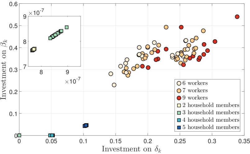
Figure 1: Correction versus prevention per node. Circle: Workers. Square: non-Workers. The color of markers indicate the size of Workplaces/Households where agents belong to.

Fig. 1 is a scatter plot showing the relationship between the investments on $\delta_{k}$ (corrective actions) and $\beta_{k}$ (preventive actions) for each agent. We can see that, in order to maximize the effectiveness of our budget, we need to invest heavily on Workers, in particular on those belonging to larger Workplaces. Figs. 2 and 2 show the infection probabilities $x_{k}$ starting from $t=t_{0}=8$, when Workers start working (therefore $\sigma(t_{0})=3$). We choose the vector of initial probabilities of infection, $x_{k}(t_{0})$, at random from the set $\{0,1\}^{N}$. Each solid curve in the figures represents the evolution in the probability of infection of an agent over time. The dashed vertical lines indicate the times when the graph changes. We are also including a dashed curve representing $E[\lVert x(t)\rVert]$ when $\sigma$ follows the Markov process with the infinitesimal generator (26).

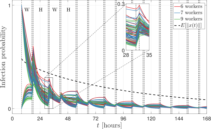
(a) Infection probabilities of Workers.

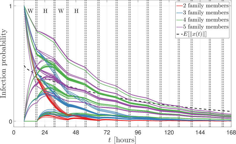
(b) Infection probabilities of non-Workers.

Figure 2: Solid: Infection probabilities $x_{k}(t)$ of Workers (2) and non-Workers (2). Dotted: $E[\lVert x(t)\rVert_{1}]$. The colors of the lines indicate the size of Workplaces/Households where agents belong to. The labels ’W’ and ’H’ indicate the first two time-periods when Workers are in their Workplaces and Households, respectively. Narrow vertical stripes represent the time-periods when Workers are commuting.

In the second example, we randomly set $\epsilon_{k}$ to be either $0$ or $1$ for each $k\in\mathcal{V}$, and solve the Performance-Constrained Disturbance Attenuation problem with the constraint $\sup_{w\in\mathcal{L}_{1}(\mathbb{R}_{+},\mathbb{R}_{+}^{N})}(\lVert E[\mathbf{x}]\rVert_{\mathcal{L}_{1}}/\lVert\mathbf{w}\rVert_{\mathcal{L}_{1}})<\gamma=40$. We use the same cost functions as in our first example. Using Theorem 3, we obtain the optimal values of $\beta_{k}$ and $\delta_{k}$ with a total cost of $67.81$. Fig. 3 is a scatter plot showing the relationship between the investments on $\delta_{k}$ and $\beta_{k}$. We can observe different patterns of resource allocation for agents with and without disturbance; in general, those with disturbance receive more allocation for corrective resources, while those without disturbance do more for preventive resources.

Before closing this section, we briefly discuss the computational cost of solving the geometric programs in this example. For simplicity, we assume that the number of nonzero entries in each column of $\Pi$ is less than or equal to $N$. Then, according to the notation in Proposition 3, we can show that $n=N(M+2)$, $k\leq 2N$, and $m\leq N(M+4)$ for Problem 1. Therefore, by Proposition 3, the computational cost for solving Problem 1 equals $O(N^{7/2}M^{7/2})$. Similarly, we can show that the same computational cost is required by the Performance-Constrained Disturbance Attenuation problem.

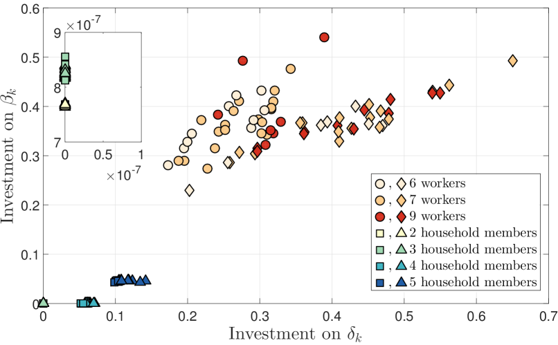
Figure 3: Correction versus prevention per node. Circle: Workers. Diamond: Workers with disturbance. Square: non-Workers. Triangle: non-Workers with disturbance. The color of markers indicate the size of Workplaces/Households where agents belong to.

VII Conclusions and Discussion

In this paper, we have proposed an optimization framework to design the subsystems and coupling elements of a time-varying network to satisfy certain structural and functional requirements. We have assumed there are both implementation costs and feasibility constraints associated with these network elements, which we have modeled using posynomial cost functions and inequalities, respectively. In this context, we have studied several design problems aiming at finding the cost-optimal network design satisfying certain budget and performance constraints, in particular, stabilization rate and disturbance attenuation. We have developed new theoretical tools to cast these design problems into geometric programs and illustrated our approach by solving the problem of stabilizing a viral spreading process in a time-switching contact network.

A possible direction for future research is the extension to networks of nonpositive systems. The proposed framework is not directly applicable to this case due to the positivity constraint in geometric program. However, by applying the framework to the upper-bounding linear dynamics of vector Lyapunov functions presented in [11], we may be still able to accomplish an efficient, if not optimal, network design for stabilization and disturbance attenuation.

Masaki Ogura received his B.Sc. degree in Engineering and M.Sc. degree in Informatics from Kyoto University, Japan, in 2007 and 2009, respectively, and his Ph.D. degree in Mathematics from Texas Tech University in 2014. He is currently a Postdoctoral Researcher in the Department of Electrical and Systems Engineering at the University of Pennsylvania. His research interest includes dynamical systems on time-varying networks, switched linear systems, and stochastic processes.

Victor M. Preciado received the Ph.D. degree in Electrical Engineering and Computer Science from the Massachusetts Institute of Technology, Cambridge in 2008. He is currently the Raj and Neera Singh Assistant Professor of Electrical and Systems Engineering at the University of Pennsylvania. He is a member of the Networked and Social Systems Engineering (NETS) program and the Warren Center for Network and Data Sciences. His research interests include network science, dynamic systems, control theory, and convex optimization with applications in socio-technical networks, technological infrastructure, and biological systems.

References

• [1] C. Asavathiratham, S. Roy, B. Lesieutre, and G. Verghese, “The influence model,” IEEE Control Systems Magazine, vol. 21, no. 6, pp. 52–64, 2001.
• [2] G. P. Barker, A. Berman, and R. J. Plemmons, “Positive diagonal solutions to the Lyapunov equations,” Linear and Multilinear Algebra, vol. 5, no. 4, pp. 249–256, 1978.
• [3] L. Benvenuti and L. Farina, “Positive and compartmental systems,” IEEE Transactions on Automatic Control, vol. 47, no. 2, pp. 370–373, 2002.
• [4] P. Bolzern, P. Colaneri, and G. De Nicolao, “Stochastic stability of Positive Markov Jump Linear Systems,” Automatica, vol. 50, pp. 1181–1187, 2014.
• [5] S. Boyd, S.-J. Kim, L. Vandenberghe, and A. Hassibi, “A tutorial on geometric programming,” Optimization and Engineering, vol. 8, no. 1, pp. 67–127, 2007.
• [6] J. Brewer, “Kronecker products and matrix calculus in system theory,” IEEE Transactions on Circuits and Systems, vol. 25, no. 9, pp. 772–781, 1978.
• [7] C. Briat, “Robust stability and stabilization of uncertain linear positive systems via integral linear constraints: $L_{1}$-gain and $L_{\infty}$-gain characterization,” International Journal of Robust and Nonlinear Control, 2012.
• [8] O. L. V. Costa, M. D. Fragoso, and M. G. Todorov, Continuous-time Markov Jump Linear Systems.   Springer, 2013.
• [9] Y. Ebihara, D. Peaucelle, and D. Arzelier, “$L_{1}$ gain analysis of linear positive systems and its application,” IEEE Conference on Decision and Control and European Control Conference, pp. 4029–4034, 2011.
• [10] L. Farina and S. Rinaldi, Positive Linear Systems: Theory and Applications.   Wiley-Interscience, 2000.
• [11] M. Ikeda and D. Šiljak, “On decentrally stabilizable large-scale systems,” Automatica, vol. 16, no. 3, pp. 331–334, 1980.
• [12] P. D. Leenheer, D. Angeli, and E. D. Sontag, “Monotone chemical reaction networks,” Journal of Mathematical Chemistry, vol. 41, no. 3, pp. 295–314, 2007.
• [13] A. Nemirovskii, “Interior Point Polynomial Time Methods in Convex Programming,” lecture notes, 2004. [Online]. Available: http://www2.isye.gatech.edu/~nemirovs/Lect_IPM.pdf
• [14] M. Ogura, “Mean Stability of Switched Linear Systems,” Ph.D. dissertation, Texas Tech University, 2014.
• [15] M. Ogura and C. F. Martin, “Stability analysis of positive semi-Markovian jump linear systems with state resets,” SIAM Journal on Control and Optimization, vol. 52, pp. 1809–1831, 2014.
• [16] M. Ogura and V. M. Preciado, “Cost-optimal switching protection strategy in adaptive networks,” to appear in 54th IEEE Conference on Decision and Control, 2015.
• [17] ——, “Disease spread over randomly switched large-scale networks,” in 2015 American Control Conference, 2015, pp. 1782–1787.
• [18] V. M. Preciado, M. Zargham, C. Enyioha, A. Jadbabaie, and G. Pappas, “Optimal vaccine allocation to control epidemic outbreaks in arbitrary networks,” in 52nd IEEE Conference on Decision and Control, 2013, pp. 7486–7491.
• [19] V. M. Preciado, M. Zargham, C. Enyioha, A. Jadbabaie, and G. J. Pappas, “Optimal resource allocation for network protection against spreading processes,” IEEE Transactions on Control of Network Systems, vol. 1, no. 1, pp. 99–108, 2014.
• [20] A. Rantzer, “Scalable control of positive systems,” European Journal of Control, vol. 24, pp. 72–80, 2015.
• [21] R. Shorten, F. Wirth, and D. Leith, “A positive systems model of TCP-like congestion control: asymptotic results,” IEEE/ACM Transactions on Networking, vol. 14, no. 3, pp. 616–629, 2006.
• [22] T. Tanaka and C. Langbort, “The bounded real lemma for internally positive systems and H-infinity structured static state feedback,” IEEE Transactions on Automatic Control, vol. 56, no. 9, pp. 2218–2223, 2011.
• [23] P. Van Mieghem, J. Omic, and R. Kooij, “Virus spread in networks,” IEEE/ACM Transactions on Networking, vol. 17, no. 1, pp. 1–14, 2009.
• [24] A. H. Zemanian, Distribution Theory and Transform Analysis.   McGraw-Hill, New York, 1965.
• [25] S. Zhu, Q.-L. Han, and C. Zhang, “$l_{1}$-gain performance analysis and positive filter design for positive discrete-time Markov jump linear systems: A linear programming approach,” Automatica, vol. 50, no. 8, pp. 2098–2107, 2014.