Technical Report
Classifying Unrooted Gaussian Trees under Privacy Constraints

Abstract

In this work, our objective is to find out how topological and algebraic properties of unrooted Gaussian tree models determine their security robustness, which is measured by our proposed max-min information (MaMI) metric. Such metric quantifies the amount of common randomness extractable through public discussion between two legitimate nodes under an eavesdropper attack. We show some general topological properties that the desired max-min solutions shall satisfy. Under such properties, we develop conditions under which comparable trees are put together to form partially ordered sets (posets). Each poset contains the most favorable structure as the poset leader, and the least favorable structure. Then, we compute the Tutte-like polynomial for each tree in a poset in order to assign a polynomial to any tree in a poset. Moreover, we propose a novel method, based on restricted integer partitions, to effectively enumerate all poset leaders. The results not only help us understand the security strength of different Gaussian trees, which is critical when we evaluate the information leakage issues for various jointly Gaussian distributed measurements in networks, but also provide us both an algebraic and a topological perspective in grasping some fundamental properties of such models.

1 Introduction

In this work, we are interested in the problem of effectively extracting maximum amount of common randomness through public discussions between Alice and Bob. based on their locally measured and correlated random variables [1, 2, 3]. Such a goal shall be attained in the presence of an eavesdropper, Eve, whose observations are also correlated with those possessed by Alice and Bob. Such scenarios are pervasive in cases where a secret key is to be established between Alice and Bob by tapping into randomness available in their surrounding physical world. For example, in a sensor network with $n$ nodes, whose local readings on, for instance, temperature or humidity, are dependent following certain joint probability distribution function, Alice and Bob have to decide which two variables $A$ and $B$ out of $N$ nodes are to be selected, whose realizations are to be used for building a secret key against a passive attack by Eve. The eavesdropper has full access to $Z$, one of the remaining $N-2$ nodes/variables, as well as those publicly exchanged messages between Alice and Bob, who establish secrecy by following the protocols proposed in [1, 2, 3] including both information reconciliation and privacy amplification stages. It has been already shown in [1, 2, 3] for a given selected three variables $A$, $B$ and $Z$, the number of bits per channel use that are information theoretically secure is proved to be $I(A;B|Z)$, the conditional mutual information between $A$ and $B$, given $Z$.

In this work, we are particularly interested in the following two questions: (1) If the joint probability distribution of $n$ random variables is representable using certain graphical models, what variables Alice and Bob should pick, subject to Eve’s selection of $Z$. (2) How should we compare and evaluate the strength of multiple graphical models in terms of the need of extracting secret key bits by Alice and Bob? To address the questions raised above, we have adopted a pessimistic approach in that Alice and Bob move first by choosing the two variables $A$ and $B$ out of $n$ variables, and thereafter Eve chooses the variable $Z$ from the remaining ones to minimize the resulting conditional mutual information. Consequently, the selection of $A$ and $B$ is thus to maximize the minimum value, which yields the solution to the corresponding maxmin problem, thereby providing the answer to the first question, under a given graphical model. For the second question, we compare different graphical models based on their respective maxmin values of the conditional mutual information. It should be noted that such a modeling has been coined as the security game in several contexts [4]. In fact, the authors in [4] define the secrecy capacity metric similar to our defined metric, which quantifies the maximum rate of reliable information transmitted from the source to destination, in presence of the eavesdropper.

Due to the vast parameter space of graphical models, we restrict our attention in this work to a set of joint probability distribution functions of $n$ variables whose conditional independence relationships can be featured in Gaussian trees to address the aforementioned problems. The Gaussian models have been extensively used in a variety of topics. In fact, recently some fundamental properties of Gaussian graphical models have been tackled using algebraic methods [5], [6]. In [5] the author shows that when the underlying random variables are Gaussian, conditional independence statements can be interpreted as algebraic constraints on the parameter space of the global model. Also, in our previous study [7], we proved that under the above assumptions, Alice, Bob and Eve form special relations with respect to each other.

To address the question of comparing different Gaussian trees in terms of their associated maximin values of the conditional mutual information, we first impose a constraint on the set of joint distributions we consider by requiring them to share the same joint entropy, i.e. the same total amount of randomness, and then we need to extensively study some fundamental properties of certain classes of unrooted Gaussian tree models related to our proposed security and privacy metrics. In particular, we propose a grafting operation [8], to transform one Gaussian tree to another by moving specific edges. Using grafting, we establish a binary relationship between Gaussian trees to determine the level of privacy, and further obtain an ordering for Gaussian trees.

In [7] we showed that for Gaussian trees with $n=\{4,5\}$ nodes, the Linear model has the largest maximin value, hence it is the most secure model for smaller size networks, which enables us to attain a full ordering for both of the cases. In this paper, we consider any general class of Gaussian tree. We prove that unlike the cases of small size Gaussian trees, for $n\geq 6$, not all the structures can be fully ordered using grafting operation. Hence, we propose partially ordered sets (posets) [9] containing tree structures, where some of the structures can be compared with each other using the binary relationship and the others are not comparable. Moreover, in order to model the Gaussian trees and the corresponding posets more systematically, we also study the algebraic properties of unrooted Gaussian tree models. Lastly, For MF trees from all posets, we show that enumerating these poset leaders can be related to integer partitions [10]. In particular, under a set of proposed principles, we can efficiently and directly enumerate all poset leaders without going through the iterative grafting operations. These structures, are specifically important, since they are the most secure trees in their related posets.

The paper is organized as follows. Section 2 presents the system model. We study the topological and algebraic properties of Gaussian trees in Sections 3 and 4. Section 5 gives the concluding remarks.

2 System Model

In this study, we consider the Gaussian joint density to capture the density of $n$ entities in a public channel, i.e., $P_{\boldsymbol{x}}(x_{1},x_{2},...,x_{n})\sim\emph{N}(\mu,\Sigma)$, where $\mu=0$ is the mean vector and $\Sigma$ is the symmetric, positive-definite covariance matrix of $n$ random variables. Furthermore, we assume that the joint density can be characterized by a weighted and unrooted tree $T=(V,E,W)$, where $V$ is the set of vertices/variables, and $E$ is the set of edges showing the dependency relations between variables [11, 5, 6]. For a fair comparison between any two Gaussian tree, we assume that the users in all models have the same joint randomness, i.e., the same entropy. In this case, it is shown that the entropy of $\boldsymbol{x}=(x_{1},x_{2},...,x_{n})$ can be obtained by $H=1/2\ln((2\pi e)^{n}|\Sigma|)$ [12]. Hence, in order to obtain a fixed entropy we have to fix the determinant of the covariance matrix, i.e., $|\Sigma|=k$, where $k\in\mathbb{R}$ is a finite and non-zero constant. In addition, similar as in [11] we assume normalized diagonal entries for the covariance matrix. This assumption, simplifies the subsequent analysis, and as we will observe, gives rise to a more compact and manageable results. On the other hand, note that normalization of diagonal entries does not change the dependency relations in a Gaussian tree. This condition makes the off-diagonal entries of $\Sigma$ to be in the range $(-1,1)$, and $k\in(0,1)$. Also, given a covariance matrix with normalized diagonal entries, the edge-weights of the Gaussian tree $T$ correspond to the covariance elements in $\Sigma$. In particular, for any edge $e_{ij}\in E$, and its associated weight $w_{ij}\in W$, we have $w_{ij}=\sigma_{ij}$, where $\sigma_{ij}$ is the $(i,j)$-th element of the covariance matrix $\Sigma$. Also, under these conditions, the covariance value between any given pair of nodes $i,j\in V$, given their connecting path $p_{ij}=e_{i,i+1}e_{i+1,i+2}...e_{j-1,j}$, is $\sigma_{ij}=w_{i,i+1}w_{i+1,i+2}...w_{j-1,j}$. In other words, the covariance value $\sigma_{ij}$ is the product of edge-weights on the path $p_{ij}$ [13].

Here, we first give a proper definition for the max-min problem, under the explained scenario.

Definition 1.

Under the Gaussian tree model, legitimate entities Alice and Bob pick two nodes $a$ and $b$ on the tree under the attack by an eavesdropper Eve who selects the third and distinct node/variable $z$ on the same tree. The objective of Alice and Bob is to select the pair $(a,b)$ to maximize the minimum conditional mutual information $I(a;b|z)$. As a result, we adopt $\max_{\{a,b\}}\min_{z}I(a;b|z,T)$ as a metric to measure the privacy level of a given weighted Gaussian tree $T=(V,E,W)$.

For Gaussian random variables the conditional mutual information $I(a;b|z)$ can be directly related to the partial correlation coefficient, which is defined as below [13],

$$\rho^{2}_{ab|z}=\dfrac{(\sigma_{ab}-\sigma_{az}\sigma_{bz})^{2}}{(\sigma_{aa}-\sigma_{az}\sigma_{az})(\sigma_{bb}-\sigma_{bz}\sigma_{bz})}=1-e^{-2I(a;b|z)}$$ (1)

where $\sigma_{ab}=E[(a-\mu_{a})(b-\mu_{b})]$, the $(a,b)$-th element of $\Sigma$, is the covariance value between variables $a$ and $b$ (with both of them having zero mean). From (1), we can see that the conditional mutual information is a monotone increasing function of the partial correlation coefficient. Hence, in the following, we use partial correlation coefficient instead of the conditional mutual information as the security and privacy metric. Hence, the corresponding max-min value for a given Gaussian tree $T=(V,E,W)$ can be restated as:

$$S(T,W)=\max_{\{a,b\}}\min_{z}\rho^{2}_{(ab|z,T,W)}$$ (2)

which is used to compare and order different trees.

3 Topological Properties of Gaussian Trees

We first define the grafting operation on Gaussian trees. In [8], the author proposes an operation called grafting to order trees based on their algebraic connectivity, which is basically the second smallest eigenvalue ($\lambda_{2}$) of the Laplacian matrix. Here, we introduce a new operation on Gaussian trees to obtain the ordering among different structures. Since, our proposed operation is similar to the grafting operation introduced in [8] (but, obviously in a totally different concept), we use the same naming to define our favorite operation.

Definition 2.

Consider a tree $T$, and assume there exists a leaf edge $e$, between the vertices $n_{1}$ and the leaf $n_{2}$. The node $n_{1}$ has degree two. The grafting operation refers to cutting the edge $e$ and attaching it to the other end of its parent edge, i.e. $e^{\prime}$, as shown in Figure 1.

Note that since grafting is essentially a local operation, only the edge $e$ changes its position: In $T_{1}$ there is an edge $e$ between the pair $\{n_{1},n_{2}\}$, while in $T_{2}$ this edge is between the pair $\{v,n_{2}\}$. All other structures shown in Figure 1 (including everything in the clouds) remain unchanged.

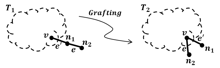
Figure 1: $T_{2}$ is obtained from $T_{1}$ by grafting operation

In [7] we showed that for any Gaussian tree the maximin value of the conditional mutual information $I(a;b|z)$ is chosen from those set of triplets in which $a$ and $b$ are adjacent and $z$ is neighbor to either $a$ or $b$. This result may seem intuitive; however, we showed that for directed Gaussian trees, there are many cases in which this result does not hold.

The computed partial correlation coefficient has the following form,

$$\rho^{2}_{ab|z}=\dfrac{\sigma^{2}_{ab}(1-\sigma^{2}_{bz})}{1-\sigma^{2}_{ab}\sigma^{2}_{bz}}$$ (3)

where the covariance values $\sigma_{ab}$ and $\sigma_{bz}$ are the corresponding weights for the edges $e_{ab}$ and $e_{bz}$, respectively. Note that in (3) we implicitly assumed $z$ is adjacent to $b$, hence if $z$ becomes adjacent to $a$, then $\sigma_{bz}$ replaces with $\sigma_{az}$ in the equation. We also proved the following result in [7],

Lemma 1.

Consider the trees $T_{1}$ and $T_{2}$ shown in Figure 1, both trees have the same set of labeling and edge weights except that the label for the weight of the edge $e$ is switched from $w_{n_{1},n_{2}}$ to $w_{v,n_{2}}$. More precisely, for $T_{2}=(V,E^{\prime},W^{\prime})$ that is obtained from $T_{1}=(V,E,W)$ using grafting operation, we know all the elements in $E^{\prime}$ and $W^{\prime}$ are the same as in $E$ and $W$, respectively, except the entry corresponding to the edge $e$. For this element we have $e^{\prime}_{v,n_{2}}=e_{n_{1},n_{2}}$ and $w^{\prime}_{v,n_{2}}=w_{n_{1},n_{2}}$. Now, suppose the maximin value for $T_{1}$, and $T_{2}$ are $S(T_{1},W)$ and $S(T_{2},W^{\prime})$, respectively. Note that $W$ is any arbitrary set of edge-weights, and $W^{\prime}$ is obtained from $W$ (by changing the covariance values associated with the grafted edge). We have $S(T_{1},W)\geq S(T_{2},W^{\prime})$.

As we can see from Lemma 1, for any given tree structure with edge-weights chosen from the corresponding entries of the covariance matrix $\Sigma$, the grafting operation always decreases the maximin value of the resulting tree. In fact, by grafting the edge $e$ we are essentially adding another neighbor to the node $n_{2}$. This in turn, gives more options to eavesdropper to choose the best location to attack, resulting in smaller maximin values. As a result, grafting operation generates a certain ordering of trees, in which the corresponding topologies are ordered with regard to their respective maximin values. In the following, we formally define the tree ordering using the results obtained in Lemma 1,

Definition 3.

Consider the trees $T_{1}=(V,E,W)$ and $T_{2}=(V,E^{\prime},W^{\prime})$, where $T_{2}$ is obtained from $T_{1}$ using grafting operation. We know from Lemma 1 that $S(T_{1},W)\geq S(T_{2},W^{\prime})$. In this setting, we write $T_{1}\succeq T_{2}$, where the binary relation $``\succeq"$ shows the ordering of these trees, i.e., $T_{1}$ is more favorable than $T_{2}$.

As we will see shortly, the ordering, which is defined in Definition 3 gives rise to developing an interesting concept: we define several classes for all Gaussian trees with the same order. Essentially, each class is a particular poset of distinct Gaussian trees.

3.1 The general cut and paste operation

We proved that for Gaussian trees with $n\in\{4,5\}$ nodes the linear topology always has largest maximin value, so it is the most secure structure [7]. However, in this paper we prove that for $n\geq 6$ this is not the case. We have the following results,

We have the following result,

Lemma 2.

Consider any Gaussian tree $T=(V,E,W)$, with order $|V|=n$. We denote $|\Sigma_{T}|$ as the determinant of covariance matrix corresponding to $T$. Considering the PG operation shown in Figure 2, which transforms the Gaussian tree $T_{1}$ into $T_{2}$, with $|\Sigma_{T_{1}}|=|\Sigma_{T_{2}}|$. Let us denote $\sigma_{n_{1}n_{2}}$ and $\sigma^{\prime}_{v^{\prime}n_{2}}$ as the covariance values between the pairs $(n_{1},n_{2})$ and $(v^{\prime},n_{2})$ in trees $T_{1}$ and $T_{2}$, respectively; then we have $\sigma^{2}_{n_{1}n_{2}}/\sigma_{n_{1}n_{1}}=\sigma^{\prime 2}_{v^{\prime}n_{2}}/\sigma_{vv}$.

Proof.

See Appendix A. ∎

Proposition 1.

Consider the trees shown in Figure 2. Given a Gaussian tree $T_{1}=(V,E,W)$, with leaf edge $e$, which is connected to $e^{\prime}$ if we cut $e$ and paste it to some vertex other than $v$ (unlike grafting), say $v^{\prime}$, we obtain the Gaussian tree $T_{2}=(V,E^{\prime},W^{\prime})$. Then, in general $T_{1}\nsucceq T_{2}$. Hence, in general $T_{1}$ is not always more favorable than $T_{2}$.

Proof.

See Appendix B. ∎

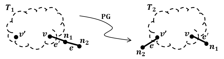
Figure 2: The figure showing the conditions in Proposition 1

From Proposition 1 we can see that if two trees are not related through one or more grafting operations, then in general they cannot be ordered using our defined binary relation. In fact, without assigning a specific covariance matrix (hence the set of edge-weights) these structures cannot be consistently compared. Since not all tree topologies can be obtained from the linear structure using grafting, so the linear topology is not always the most secure structure. This result motivates us to seek for certain topologies that cannot be compared with each other, and at the same time they cannot be improved further, using grafting operation. In particular, we form sets of tree structures, where each set contains a unique leader that is the most favorable topology among all other topologies in the same set. Other topologies in a poset might be comparable/incomparable with each other. By classifying the trees into certain sets we can further study both their topological and algebraic properties.

3.2 Forming the posets of Gaussian trees

Based on the obtained results in Proposition 1 we can form posets [9] of Gaussian trees. Each poset is formed from its most favorable (MF) structure, $T_{M}=(V_{M},E_{M},W_{M})$. In other words, $T_{M}$ is the poset leader acting as the ancestor to all other Gaussian trees in a poset, i.e., all other Gaussian trees can be obtained from $T_{M}$ using one or more grafting operations. Also, in each poset given two trees $T_{i}$ and $T_{j}$, they are adjacent if $T_{j}$ can be obtained from $T_{i}$ by grafting one of its edges. In this case, there is a directed edge from $T_{i}$ to $T_{j}$, i.e. $T_{i}\rightarrow T_{j}$.

Lemma 3.

In any poset with a given $T_{M}=(V_{M},E_{M},W_{M})$ acting as a poset leader, we can find a unique least favorable (LF) structure, $T_{L}=(V_{L},E_{L},W_{L})$, which acts as a descendant to all other trees.

Proof.

See Appendix C ∎

Hence, we observe that our defined posets are certain class of posets, which have a unique MF ans LF structures. Also, from the results in Lemma 1 we know that $T_{M}$ has the most secure structure, while $T_{L}$ has the least secure structure in each poset. As an example, Figure 3 shows all three posets of Gaussian trees on $7$ nodes. It can be seen that when there is a directed path between two topologies, then they are comparable using our defined binary relation. Note that in this figure, posets $1$ and $3$ are the special cases where posets are basically formed as fully ordered sets, hence any tree structure in each of these poset can be compared to other trees in the same poset. On the other hand, in poset $2$, the two middle structures cannot be compared using the rules given in Lemma 1. Also, the MF and LF structures are placed at the top and bottom of each poset, respectively.

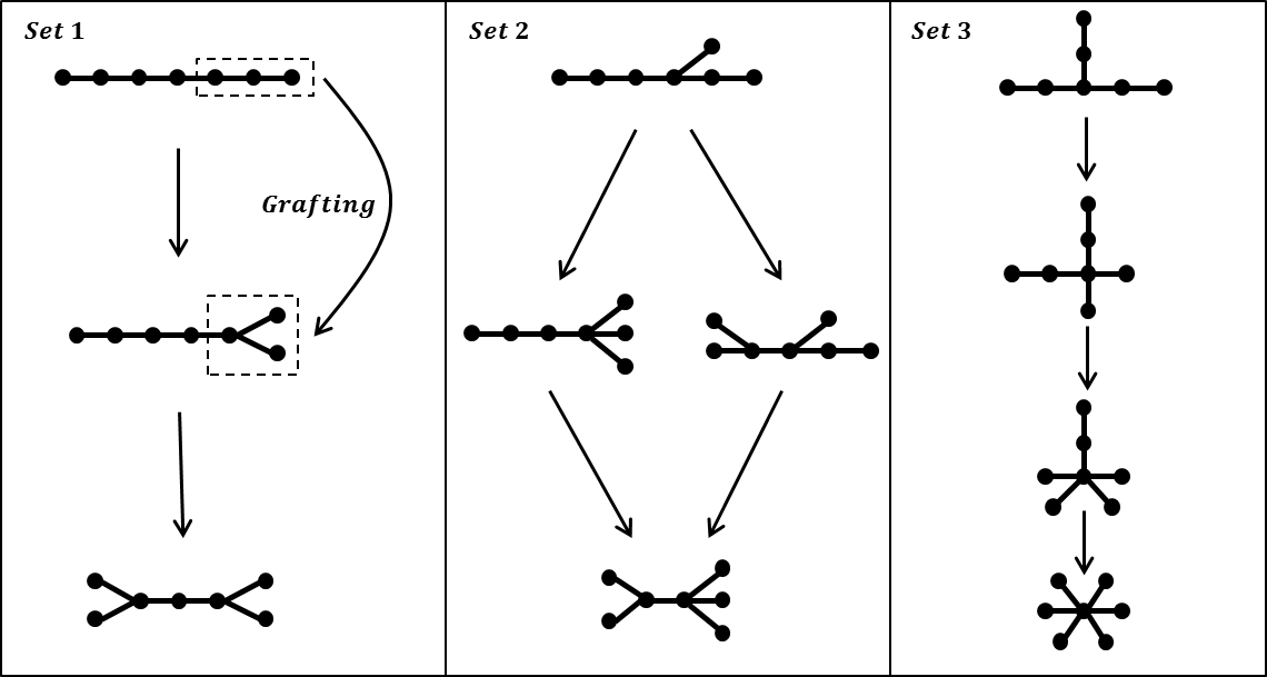
Figure 3: All the possible posets for Gaussian trees with $n=7$ nodes

The MF topologies are the most secure trees in each poset; also as we observed, poset leaders can characterize all other structures in a poset: the poset leaders can fully describe the poset structure. Hence, finding such structures is of huge importance. However, there should be a method to systematically obtain these topologies. Thus, in section 4 we propose an efficient way, which can enumerate all these structures systematically.

3.3 Forming the super-graph for each poset

Figure 3 gives us an intuition in order to construct a directed super-graph containing Gaussian trees. In particular, each poset can be converted into a directed super-graph $G=(V_{s},E_{s})$, where $V_{s}$ is the set of trees in a poset acting as vertices, and $E_{s}$ is the set of directed edges between the two nodes that can be related using grafting. Using this super-graph, we can easily identify the comparable tree structures: If there is a directed path between two structures, then they are comparable. Hence, we can conclude that both MF and LF structures can be compared with any other tree in a poset. Also, observe that poset leader fully characterizes the structure of its super-graph. In particular, the number of those leaf edges (in the poset leader structure) that are adjacent to a particular node with degree two, specifies the length (number of consecutive grafting operations plus $1$) of the super-graph. Moreover, the structure of those special edges specifies the width of the super-graph. In particular, consider the following: in Figure 3 we can see that the poset $3$ have three special edges, hence the super-graph has length $4$. Also, since these special edges are fully symmetric with respect to each other (grafting either of those edges, results in a same tree), so the poset $3$ becomes fully ordered. On the other hand, in poset $2$ because of the two asymmetric branches we obtain two different topologies in the next level. In general, if those special branches become more symmetric, the poset tends to become fully ordered.

Although, converting each poset to its corresponding super-graph simplifies the comparison between tree topologies in a set, but as it can be observed, for larger trees identifying these special branches and ordering trees by grafting operation becomes more challenging. Hence, in the following we aim to study the tree structures and their associated posets in a more abstract and general ways.

4 Algebraic properties of Gaussian Trees

4.1 Tutte-Like Polynomials for Gaussian Trees in Posets

In this section, in order to model the Gaussian trees and the corresponding posets more systematically, we study the algebraic properties of these models. As we may see in the following, these properties will further help us characterize those special leaf nodes with no leaf siblings, and thus allow us to evaluate the security robustness of any tree structure within a poset. To achieve this goal, for each tree, we associate a two-variable Tutte-like polynomial defined in [14], where the authors modify the definition of the Tutte polynomial to obtain a new invariant for both rooted and unrooted trees. Also, they proved that this polynomial uniquely determines rooted trees. For unrooted trees however, it is shown in [15] that certain classes of caterpillars have the same polynomials assigned to them. However, interestingly, we prove that in each poset, in many cases the trees have unique polynomials.

Let $R(T)$ denote the collection of all subtrees of $T$, and $L_{E}(S)$ denote the leaf edges in the subtree $S$, i.e., the edges that are connected to leaf nodes then [14],

$$f_{E}(T;t,z)=\sum_{S\subseteq R(T)}t^{|E(S)|}(z+1)^{|E(S)|-|L_{E}(S)|}$$ (4)

where $|E(S)|$ is the total number of edges in the subtree $S$. Basically, this polynomial is a generating function that encodes the number of subtrees with a given internal and leaf edges [15]. We next show that such polynomials can help us systematically generate trees in a poset from the poset leader. The proof can be found in Appendix D.

Lemma 4.

Suppose there is a directed path from the tree $T_{n}$ to $T_{n-m}$ in a poset, i.e., $T_{n-m}$ can be obtained from $T_{n}$ through $m$ grafting operation. Then, their associated polynomials have the following recursive formula,

$$f(T_{n}; t,z)=$$

$$f(T_{n-m};t,z)+t(1-tz)[m-\sum_{k=1}^{m}g_{n-k}(t,z)]$$ (5)

where, $g_{n-k}(t,z)$ is the polynomial associated to the rooted tree obtained from the tree $T_{n-k}$, after deleting the edges $e$ and its neighbor edge $e^{\prime}$ (e.g., see $e$ and $e^{\prime}$ shown in Figure 1 for the tree $T_{1}$), in a given step $k$, and putting their common node as a root (e.g., the node $v$ in Figure 1). Note that in (4), $T_{1}$ is the LF topology.

Using the recursive equation derived in (4), we then have the following corollary, whose proof is in Appendix E.

Corollary 1.

In a poset, certain tree structures are uniquely determined by Tutte-like polynomial. In particular, if one of the following cases happen then two polynomials are distinct: (1) If there exists a directed path between two trees; (2) If both trees have the same parent tree; (3) If the two structures lie at different levels.

Hence, by Corollary 1 we see that although Tutte-like polynomial is not graph invariant in general, but in many cases the polynomials associated to trees in a same poset are distinct. As an example, consider the poset $2$ shown in Figure 3. Since all trees satisfy at least one of the conditions in Corollary 1, all of their associated polynomials are thus be distinct. Following (4), we have

$$f(T_{M};t,y)=t^{6}y^{3} +t^{5}(y^{3}+2y^{2})+t^{4}(3y^{2}+2y)$$

$$+t^{3}(5y+1)+6t^{2}+6t+1$$

$$f(T_{l};t,y)=t^{6}y^{2} +t^{5}(3y^{2}+y)+t^{4}(3y^{2}+3y+1)$$

$$+t^{3}(4y+4)+8t^{2}+6t+1$$

$$f(T_{r};t,y)=t^{6}y^{2} +t^{5}(3y^{2}+y)+t^{4}(2y^{2}+5y)$$

$$+t^{3}(6y+2)+7t^{2}+6t+1$$

$$f(T_{L};t,y)=t^{6}y +5t^{5}y+t^{4}(8y+1)+t^{3}(6y+5)$$

$$+9t^{2}+6t+1$$ (6)

where $T_{M}$ and $T_{L}$ are the MF and LF topologies in poset $2$, respectively. Also, $T_{l}$ and $T_{r}$ are the left and right topologies, respectively that located in the middle of poset $2$. For the simplicity of polynomials we replaced $z+1$ with $y$. As we expect, all the computed polynomials in (4.1) are distinct.

The Tutte-like polynomial can be used to evaluate certain topological properties of trees. In the following lemma, whose proof is in Appendix F, we propose an interesting result: the Tutte-like polynomial can enable us to extract the exact number of those special leaf edges from this polynomial. Hence, using this result we estimate the security robustness of a tree structure by computing its distance from LF structure.

Lemma 5.

Given the polynomial $f(T;t,z)$ associated with $T$, the second highest degree term has the form $t^{|E|-1}(\alpha(1+z)^{|I|-1}+\beta(1+z)^{|I|})$. The coefficient $\alpha$ shows the number of leaf edges with no leaf siblings.

Corollary 2.

The coefficient $\alpha$ defined in Lemma 5 shows the distance between the tree $T$ and LF structure. Also, if $\alpha=0$ then $T$ is the LF structure.

Example 1.

Consider the tree topologies in poset $2$ of Figure 3, and their associated polynomials that is computed in (4.1). The MF tree $T_{M}$ has two leaf edges with no siblings, hence in its corresponding polynomial, the second highest degree term has the form $t^{5}y^{3}+2t^{5}y^{2}$. Hence, $\alpha=2$. On the other hand, the LF tree $T_{L}$ has no such leaf edges. From (4.1) we can see the second highest degree term for $f(T_{L};t,y)$ is $5t^{5}y$, hence $\alpha=0$.

The results obtained in Lemma 5 and Corollary 2 show the strong correlation between the Tutte-like polynomial and security robustness of Gaussian tree. This information is very helpful in order to compare the security of a tree in a poset. In particular, being closer to LF structure, hence having smaller values for $\alpha$ (comparing to others in the same poset), makes the Gaussian tree less favorable comparing to other structures in a poset.

4.2 Enumerating Poset Leaders: Restricted Integer Partition Approach

In the previous sections, we studied certain properties of tree topologies in the same poset. In this section, we find a systematic way to generate different poset leaders, which is further related to restricted integer partition problems. The method we propose is essentially determined by the property of each MF in that the leaf edges have no leaf siblings in all MF structures. The following example will demonstrate new ways to quickly enumerate these MF models.

Consider the MF topology in poset $3$ shown in Figure 3. There are three branches coming out of the central node, which has degree $3$. Each branch has $2$ nodes, hence we assign the string $(2+2+2)$ to this topology. Each number (here all numbers are $2$) shows the length of their corresponding branches. Note that we do not count the central node, which we name it the anchor node. Similarly consider the MF topology in poset $2$, which is shown in Figure 3. Here, the anchor node is the vertex with degree $3$, hence we assign the string $(1+2+3)$ to this topology. Lastly, consider the MF topology in poset $1$. Since, all the internal nodes, can be anchor nodes, hence we can assign multiple (equivalent) strings to this topology, i.e., $(1+5)$, $(2+4)$, and $(3+3)$ are all valid strings.

Based on this example, we propose an effective algorithm (in fact, the set of constraints) to enumerate all poset leaders of given order. It turns out that integer partition methods [10] can be very helpful in order to quickly reach this goal. However, this method should be systematically implemented. In particular, we use restricted integer partitions to find all poset leaders.

Each integer partition should satisfy the following conditions: (1) Each part should have at most a single $1$ (2) The leftmost and rightmost parts should both be larger than $3$. Given $|V|=n$ we do the following until all of the parts cannot be partitioned without violating the restrictive conditions:

Enumerating Poset Leaders

$1.$ Find all integer partitions for $n-A$

$2.$ For each one of these partitions, find those parts that can be further partitioned, and follow the steps in $1$.

$3.$ Check for any redundant partitions and eliminate them, and if any permutation of parts gives a new poset leader structure

Here $A$ shows the number of anchor nodes. Basically, in the above set of principles the first constraint is to ignore the non-poset leader cases, while the second constraint is to ignore the cases where two or more parts can be merged and form already produced parts, hence, making this method more effective. The anchor nodes are certain non-leaf vertices, acting as a hub for two or more branches. Each of the anchor nodes, with their associated branches can form a smaller integer partition satisfying the aforementioned constraints. Also, unlike normal integer partitions the position of parts matters, so we should count some of permutations of different parts. In particular, two non-isomorphic poset leader topologies may have identical integer partitions, but with different ordering of parts.

5 Conclusion

In this paper, we analyzed the information leakage in public communications channels, where the joint density of entities in the channel can be modeled by Gaussian trees. We addressed two fundamental problems: $(1)$ In the max-min scenario we showed the special relation between $3$ variables that are be chosen by Alice, Bob, and Eve. $(2)$ Under the same scenario, we studied the impact of choosing different structures, on the maximin value and hence on the channel security. We proposed the grafting operation, which produces less favorable trees. Then, we ordered the tree structures using our defined pair-wise relationship. Interestingly, using our defined operation, we obtained partially ordered sets of trees, through which we classified all the Gaussian tree structures of given order into several partially ordered sets. We proved a particular feature for the sets: each poset have a unique MF and LF structures. In order to further simplify comparing topologies, we modeled each poset as a directed super-graph, by which any two trees are comparable if there is a directed path from one to the other. Moreover, we provided a systematic way of producing all trees in a poset through computing corresponding Tutte-like polynomials. We obtained certain fundamental results: using the second highest degree term in each polynomial one can evaluate the security robustness of the given structure. Lastly, we introduced a restricted integer partition approach based on proposed principles to quickly enumerate all poset leaders of a given order without listing all non-leader structures.

Appendix A Proof of Lemma 2

We first prove the following:

For any $v_{i}\in V$, let us define $d_{i}$ as its degree. Then, we have,

$$|\Sigma_{T}|=\dfrac{\prod\limits_{(v_{i},v_{j})\in E}[\sigma_{v_{i}v_{i}}\sigma_{v_{j}v_{j}}-\sigma^{2}_{v_{i}v_{j}}]}{\prod\limits_{v_{i}\in V}\sigma_{v_{i}v_{i}}^{d_{i}-1}}$$ (7)

The proof follows by induction. First, assume that the Gaussian tree $T$ has only one edge with two vertices $v_{1}$ and $v_{2}$, then we can immediately form $\Sigma_{T}$, and deduce $|\Sigma_{T}|=\sigma_{v_{1}v_{1}}\sigma_{v_{2}v_{2}}-\sigma^{2}_{v_{1}v_{2}}$, which follows the general formula in (7). Next, let us assume that (7) is valid up to $T^{\prime}=(V^{\prime},E^{\prime},W^{\prime})$, where $|V^{\prime}|=n-1$. Hence, we need to prove the validity of this equation for $T=(V,E,W)$ with $|V|=n$, where the tree $T$ can be obtained from $T^{\prime}$ by adding one vertex, namely $v_{n}$. Without loss of generality, we assume that $v_{n}$ is connected to $v_{n-1}$. Since $v_{n}\perp v_{i}|v_{n-1}$, for all $v_{i}\in V\backslash\{v_{n},v_{n-1}\}$, using the arguments given in Section 2, we have $\sigma_{v_{i}v_{n}}=\sigma_{v_{i}v_{n-1}}\sigma_{v_{n-1}v_{n}}/\sigma_{v_{n-1}v_{n-1}}$. If we factorize ${\sigma_{v_{n-1}v_{n}}}/{\sigma_{v_{n-1}v_{n-1}}}$ from the last column, then subtract the $n-1$-th column from the $n$-th column, and replace the result with the $n$-th column, we obtain,

$$|\Sigma_{T}|=\dfrac{\sigma_{v_{n-1}v_{n}}}{\sigma_{v_{n-1}v_{n-1}}}\begin{vmatrix}\sigma_{v_{1}v_{1}}&\cdots&0\\ \sigma_{v_{2}v_{1}}&\cdots&0\\ \vdots&\ddots&\vdots\\ \sigma_{v_{n-1}v_{1}}&\cdots&0\\ \sigma_{v_{n}v_{1}}&\cdots&x\end{vmatrix}$$

where $x=(\sigma_{v_{n}v_{n}}\sigma_{v_{n-1}v_{n-1}}-\sigma^{2}_{v_{n}v_{n-1}})/\sigma_{v_{n}v_{n-1}}$. Using the last column, we can compute $|\Sigma_{T}|$ as follows,

$$|\Sigma_{T}| =\dfrac{\sigma_{v_{n-1}v_{n}}}{\sigma_{v_{n-1}v_{n-1}}}x|\Sigma_{\backslash n\backslash n}|$$

$$=\dfrac{\sigma_{v_{n}v_{n}}\sigma_{v_{n-1}v_{n-1}}-\sigma^{2}_{v_{n}v_{n-1}}}{\sigma_{v_{n-1}v_{n-1}}}|\Sigma_{\backslash n\backslash n}|$$ (8)

where $|\Sigma_{\backslash n\backslash n}|$ is the determinant of submatrix of $\Sigma_{T}$ resulting after removing the $n$-th column and row. Note that since removing the last row and column of $\Sigma_{T}$ is the same as removing $v_{n}$ from $T$, hence we conclude that $\Sigma_{\backslash n\backslash n}=\Sigma_{T^{\prime}}$. Therefore, (A) becomes

$$|\Sigma_{T}|=\dfrac{\sigma_{v_{n}v_{n}}\sigma_{v_{n-1}v_{n-1}}-\sigma^{2}_{v_{n}v_{n-1}}}{\sigma_{v_{n-1}v_{n-1}}}|\Sigma_{T^{\prime}}|$$ (9)

Observe that since the degree of $v_{n-1}$ is $2$, the fraction in (9) has the same form as in (7). Also, we know that $|\Sigma_{T^{\prime}}|$ follows the general formula as well. This completes the inductive proof for the first part.

To prove the result in Lemma 2, note that the Gaussian trees $T_{1}$ and $T_{2}$ differ in only one edge, namely $e$. Hence, we can write,

$$|\Sigma_{T_{1}}|=|\Sigma_{\backslash n_{2}\backslash n_{2}}|\dfrac{\sigma_{n_{1}n_{1}}\sigma_{n_{2}n_{2}}-\sigma^{2}_{n_{1}n_{2}}}{\sigma_{n_{1}n_{1}}}$$

$$|\Sigma_{T_{2}}|=|\Sigma_{\backslash n_{2}\backslash n_{2}}|\dfrac{\sigma_{v^{\prime}v^{\prime}}\sigma_{n_{2}n_{2}}-\sigma^{2}_{v^{\prime}n_{2}}}{\sigma_{v^{\prime}v^{\prime}}}$$

Since we assume that $|\Sigma_{T_{1}}|=|\Sigma_{T_{2}}|$, the result follows.

Appendix B Proof of Proposition 1

Based on the values of edge-weights, two possible cases may happen for the maximin value of the tree $T_{1}$ and $T_{2}$ that are shown in Figure 2:

Case 1.

Let’s assume $S(T_{1},W)$ consists the nodes $n_{1}$, $n_{2}$, and $v$. In particular, using (3) we obtain $S(T_{1},W)=\dfrac{\sigma^{2}_{vn_{1}}(1-\sigma^{2}_{n_{1}n_{2}})}{1-\sigma^{2}_{n_{1}n_{2}}\sigma^{2}_{vn_{1}}}$. In other words, $S(T_{1},W)$ is larger than all other partial correlations except the triplets which contain the pair $\{n_{1},v\}$ and the nodes other than $n_{2}$. Now, the maximin value of $T_{2}$, say $S(T_{2},W)$, is obtained by $S(T_{2},W^{\prime})=\max\{\min_{i}(\dfrac{\sigma^{2}_{vn_{1}}(1-\sigma^{2}_{vx_{i}})}{1-\sigma^{2}_{vx_{i}}\sigma^{2}_{vn_{1}}}),f(T_{2},W^{\prime})\}$, where $x_{i}$ are the adjacent nodes to $v$, other than $n_{1}$. Also, $f(T_{2},W^{\prime})$ can be any other value chosen from the max-min table corresponding to the tree $T_{2}$. We can show that, in any case we have $S(T_{2},W^{\prime})\geq S(T_{1},W)$.

Case 2.

If $S(T_{1},W)=\dfrac{\sigma^{2}_{v^{\prime}x^{\prime}_{i}}(1-\sigma^{2}_{x^{\prime}_{i}y^{\prime}_{j}})}{1-\sigma^{2}_{v^{\prime}x^{\prime}_{i}}\sigma^{2}_{x^{\prime}_{i}y^{\prime}_{j}}}$, where $x^{\prime}_{i}$ is adjacent to $v^{\prime}$ and $y^{\prime}_{j}$ is adjacent to $x^{\prime}_{i}$, then for $S(T_{2},W^{\prime})$, we have $S(T_{2},W^{\prime})=\min\{S(T_{1},W),\dfrac{\sigma^{2}_{v^{\prime}x^{\prime}_{i}}(1-\sigma^{2}_{v^{\prime}n_{2}})}{1-\sigma^{2}_{v^{\prime}x^{\prime}_{i}}\sigma^{2}_{v^{\prime}n_{2}}}\}$. Hence, we can conclude that $S(T_{1},W)\geq S(T_{2},W^{\prime})$.

From two above cases we can conclude that in Case 1, $T_{2}$ is more favorable than $T_{1}$, whereas in Case 2 the opposite conclusion holds.

Appendix C Proof of Lemma 3

The proof is quite straightforward. For any poset, given its poset leader $T_{M}$ we can find and graft those leaf edges with no leaf siblings. Obviously, we can begin with any list of edges with any order. Hence, in any case we end up with a unique structure, namely $T_{L}$.

Appendix D Proof of Lemma 4

By combining propositions $4$, $5$, $15$, and $18$ from [14] we can conclude the following,

$$f(T_{n};t,z)=h_{n-1}+t[t(z+1)g_{n-1}+(1-tz)]$$

$$f(T_{n-1};t,z)=h_{n-1}+t(t+1)g_{n-1}$$

where $h_{n-1}$ is the polynomial related to the unrooted tree $T_{n}/e$, i.e., the unrooted tree $T_{n}$ after deleting an edge $e$. Note that for simplicity we write $h_{n-1}$ and $g_{n-1}$ instead of $h_{n-1}(t,z)$ and $g_{n-1}(t,z)$, respectively. Using the above equations, we obtain the following recursive formula,

$$f(T_{n}; t,z)=f(T_{n-1};t,z)+t(1-tz)[1-g_{n-1}(t,z)]$$ (10)

If we proceed up to level $m$, the result in (4) follows.

Appendix E Proof of Corollary 1

First, suppose $f(T_{n};t,z)=f(T_{n-m};t,z)$ then using (4) we should have $t(1-tz)[m-\sum_{k=1}^{m}g_{n-k}(t,z)]=0$, or $\sum_{k=1}^{m}g_{n-k}(t,z)=m$. Recall that all $g_{n-k}(t,z)$ are polynomials associated with rooted trees, so the only possibility is $g_{n-k}(t,z)=1$, for all $1\leq k\leq m$, a contradiction.

Second, consider two trees $T_{n-m}$ and $T_{n-l}$, at different levels having nearest common ancestor $T_{n}$. Then using (4) we have the following:

$$f(T_{n}; t,z)=\begin{cases}f^{L}(T_{n-m};t,z)+t(1-tz)[m-\sum_{k=1}^{m}g^{L}_{n-k}]\\ f^{R}(T_{n-l};t,z)+t(1-tz)[l-\sum_{k=1}^{l}g^{R}_{n-k}]\end{cases}$$

suppose, $f^{L}(T_{n-m};t,z)=f^{R}(T_{n-l};t,z)$ then we obtain,

$$\sum_{k=1}^{m}g^{L}_{n-k}-\sum_{k=1}^{l}g^{R}_{n-k}=m-l$$ (11)

If $m=l=1$, i.e., both trees $T_{n-m}$ and $T_{n-l}$ are obtained from $T_{n}$ by a single grafting operation. But, since they have two different structures, the corresponding polynomials for the rooted trees $g^{L}_{n-1}$ and $g^{R}_{n-1}$ are distinct, because in [14] it is shown that Tutte-like polynomial for rooted trees is graph invariant. Hence, $f^{L}(T_{n-1};t,z)$ and $f^{R}(T_{n-1};t,z)$ are distinct. So, the trees at the same level that are obtained from their parent through one grafting operation are distinct.

Finally, suppose we have $m\neq l$. Let’s define $y_{i}=g_{i}-1$ for all polynomials $g_{i}(t,z)$. Now, using (11) we have,

$$\sum_{k=1}^{m}y^{L}_{n-k}-\sum_{k=1}^{l}y^{R}_{n-k}=0$$ (12)

The highest degree term corresponds to the rooted trees, resulted by eliminating the edges $e$ and $e^{\prime}$ and putting the common node between these two edges as a root. Also, the highest degree terms are resulted from the subtrees associated to $y^{L}_{i}$ and $y^{R}_{i}$ and no other proper subsets of these trees. Hence, from (12) and assuming that original tree $T_{n}$ has the size $|E|$, then we can conclude,

$$t^{|E|-2}\sum_{k=1}^{m}(1+z)^{L_{n-k}}=t^{|E|-2}\sum_{k=1}^{l}(1+z)^{R_{n-k}}$$ (13)

where $L_{n-k}$ and $R_{n-k}$ are non-negative integer powers, which show the largest number of internal edges for each tree associated to polynomials $y^{L}_{n-k}$ and $y^{R}_{n-k}$.

Equation (13) should hold for all values of $t$ and $z$. Let’s set $t=1$ and $z=0$, we obtain $m=l$, a contradiction.

Appendix F Proof of Lemma 5

The second highest degree term consists of those subtrees of $T$ with exactly one edge missing. This edge should be a leaf edge, since otherwise the resulting structure does not become a tree. Now, consider those edges that are connected to the deleted leaf edge. They either become leaf or keep their previous states. Hence, the second highest degree term has the form $t^{|E|-1}(\alpha(1+z)^{|I|-1}+\beta(1+z)^{|I|})$, where $t^{|E|-1}$ is due to the deleted edge. Also, $\alpha$ is the number of resulted subtrees with $|I|-1$ internal edges, and $\beta$ is the number of those subtrees with $|I|$ internal edges. Hence, the number of leaf edges with no leaf siblings is $\alpha$.

References

- [1] U. M. Maurer, “Secret key agreement by public discussion from common information,” Information Theory, IEEE Transactions on, vol. 39, no. 3, pp. 733–742, 1993.
- [2] R. Ahlswede and I. Csiszár, “Common randomness in information theory and cryptography. part i: secret sharing,” IEEE Transactions on Information Theory, vol. 39, no. 4, 1993.
- [3] ——, “Common randomness in information theory and cryptography. ii. cr capacity,” Information Theory, IEEE Transactions on, vol. 44, no. 1, pp. 225–240, 1998.
- [4] M. H. Manshaei, Q. Zhu, T. Alpcan, T. Bacşar, and J.-P. Hubaux, “Game theory meets network security and privacy,” ACM Computing Surveys (CSUR), vol. 45, no. 3, p. 25, 2013.
- [5] S. Sullivant, “Algebraic geometry of Gaussian Bayesian networks,” Advances in Applied Mathematics, vol. 40, no. 4, pp. 482–513, 2008.
- [6] H. Roozbehani and Y. Polyanskiy, “Algebraic methods of classifying directed graphical models,” arXiv preprint arXiv:1401.5551, 2014.
- [7] A. Moharrer, S. Wei, G. Amariucai, and J. Deng, “Evaluation of security robustness against information leakage in Gaussian polytree graphical models,” in Proceedings of the Wireless Communications and Networking Conference (WCNC), 2015 IEEE, pp. 1422–1427.
- [8] K. Patra and A. Lal, “The effect on the algebraic connectivity of a tree by grafting or collapsing of edges,” Linear Algebra and its Applications, vol. 428, no. 4, pp. 855–864, 2008.
- [9] W. T. Trotter, Combinatorics and partially ordered sets: Dimension theory. JHU Press, 2001, vol. 6.
- [10] G. E. Andrews, The theory of partitions. Cambridge university press, 1998, vol. 2.
- [11] P. Šimecek, “Gaussian representation of independence models over four random variables,” in COMPSTAT conference, 2006.
- [12] T. M. Cover and J. A. Thomas, Elements of information theory. John Wiley & Sons, 2012.
- [13] S. Chaudhuri, “Qualitative inequalities for squared partial correlations of a Gaussian random vector,” Annals of the Institute of Statistical Mathematics, vol. 66, no. 2, pp. 345–367, 2014.
- [14] S. Chaudhary and G. Gordon, “Tutte polynomials for trees,” Journal of graph theory, vol. 15, no. 3, pp. 317–331, 1991.
- [15] D. Eisenstat and G. Gordon, “Non-isomorphic caterpillars with identical subtree data,” Discrete mathematics, vol. 306, no. 8, pp. 827–830, 2006.