Detrended partial cross-correlation analysis of two nonstationary time series influenced by common external forces

Abstract

When common factors strongly influence two power-law cross-correlated time series recorded in complex natural or social systems, using classic detrended cross-correlation analysis (DCCA) without considering these common factors will bias the results. We use detrended partial cross-correlation analysis (DPXA) to uncover the intrinsic power-law cross-correlations between two simultaneously recorded time series in the presence of nonstationarity after removing the effects of other time series acting as common forces. The DPXA method is a generalization of the detrended cross-correlation analysis that takes into account partial correlation analysis. We demonstrate the method by using bivariate fractional Brownian motions contaminated with a fractional Brownian motion. We find that the DPXA is able to recover the analytical cross Hurst indices, and thus the multi-scale DPXA coefficients are a viable alternative to the conventional cross-correlation coefficient. We demonstrate the advantage of the DPXA coefficients over the DCCA coefficients by analyzing contaminated bivariate fractional Brownian motions. We calculate the DPXA coefficients and use them to extract the intrinsic cross-correlation between crude oil and gold futures by taking into consideration the impact of the US dollar index. We develop the multifractal DPXA (MF-DPXA) method in order to generalize the DPXA method and investigate multifractal time series. We analyze multifractal binomial measures masked with strong white noises and find that the MF-DPXA method quantifies the hidden multifractal nature while the MF-DCCA method fails.

I Introduction

Complex systems with interacting constituents are ubiquitous in nature and society. To understand the microscopic mechanisms of emerging statistical laws of complex systems, one records and analyzes time series of observable quantities. These time series are usually nonstationary and possess long-range power-law cross-correlations. Examples include the velocity, temperature, and concentration fields of turbulent flows embedded in the same space as joint multifractal measures Antonia and Van Atta (1975); Meneveau et al. (1990), topographic indices and crop yield in agronomy Kravchenko et al. (2000); Zeleke and Si (2004), temporal and spatial seismic data Shadkhoo and Jafari (2009), nitrogen dioxide and ground-level ozone Jiménez-Hornero et al. (2010), heart rate variability and brain activity in healthy humans Lin and Sharif (2010), sunspot numbers and river flow fluctuations Hajian and Movahed (2010), wind patterns and land surface air temperatures Jiménez-Hornero et al. (2011), traffic flows Xu et al. (2010) and traffic signals Zhao et al. (2011), self-affine time series of taxi accidents Zebende et al. (2011), and econophysical variables Lin (2008); Podobnik et al. (2009a); Siqueira Jr. et al. (2010); Wang et al. (2010); He and Chen (2011).

A variety of methods have been used to investigate the long-range power-law cross-correlations between two nonstationary time series. The earliest was joint multifractal analysis to study the cross-multifractal nature of two joint multifractal measures through the scaling behaviors of the joint moments Antonia and Van Atta (1975); Meneveau et al. (1990); Schmitt et al. (1996); Xu et al. (2000, 2007), which is a multifractal cross-correlation analysis based on the partition function approach (MF-X-PF) Wang et al. (2012). Over the past decade, detrended cross-correlation analysis (DCCA) has become the most popular method of investigating the long-range power-law cross correlations between two nonstationary time series Jun et al. (2006); Podobnik and Stanley (2008); Podobnik et al. (2009a); Horvatic et al. (2011), and this method has numerous variants Achard et al. (2008); Arianos and Carbone (2009); Wendt et al. (2009); Qiu et al. (2010, 2011); Kristoufek (2013, 2014); Ying and Shang (2014); Kristoufek (2015). Statistical tests can be used to measure these cross correlations Podobnik et al. (2009b); Zebende (2011); Podobnik et al. (2011). There is also a group of multifractal detrended fluctuation analysis (MF-DCCA) methods of analyzing multifractal time series, e.g., MF-X-DFA Zhou (2008), MF-X-DMA Jiang and Zhou (2011), and MF-HXA Kristoufek (2011).

The observed long-range power-law cross-correlations between two time series may not be caused by their intrinsic relationship but by a common third driving force or by common external factors Kenett et al. (2009); Shapira et al. (2009); Kenett et al. (2010). If the influence of the common external factors on the two time series are additive, we can use partial correlation to measure their intrinsic relationship Baba et al. (2004). To extract the intrinsic long-range power-law cross-correlations between two time series affected by common driving driving forces, we previously developed and used detrended partial cross-correlation analysis (DPXA) and studied the DPXA exponents of variable cases, combining the ideas of detrended cross-correlation analysis and partial correlation Liu (2014). In Ref. Yuan et al. (2015), the DPXA method has been proposed independently, focussing on the DPXA coefficient.

Here we provide a general framework for the DPXA and MF-DPXA methods that is applicable to various extensions, including different detrending approaches and higher dimensions. We adopt two well-established mathematical models (bivariate fractional Brownian motions and multifractal binomial measures) in our numerical experiments, which have known analytical expressions, and demonstrate how the (MF-)DPXA methods is superior to the corresponding (MF-)DCCA methods.

II Detrended partial cross-correlation analysis

II.1 DPXA exponent

Consider two stationary time series $\{x(t):t=1,\cdots,T\}$ and $\{y(t):t=1,\cdots,T\}$ that depend on a sequence of time series $\{z_{i}(t):t=1,2,\cdots,T\}$ with $i=1,\cdots,n$. Each time series is covered with $M_{s}=[T/s]$ non-overlapping windows of size $s$. Consider the $v$th box $[l_{v}+1,l_{v}+s]$, where $l_{v}=(v-1)s$. We calibrate the two linear regression models for ${\bm{x}}_{v}$ and ${\bm{y}}_{v}$ respectively,

$$\left\{\begin{array}[]{ccc}{\bm{x}}_{v}={\mathbf{Z}}_{v}{\bm{\beta}_{x,v}}+{\mathbf{r}}_{x,v}\\ {\bm{y}}_{v}={\mathbf{Z}}_{v}{\bm{\beta}_{y,v}}+{\mathbf{r}}_{y,v}\end{array}\right.,$$ (1)

where ${\mathbf{x}}_{v}=[x_{l_{v}+1},\ldots,x_{l_{v}+s}]^{\mathrm{T}}$, ${\mathbf{y}}_{v}=[y_{l_{v}+1},\ldots,y_{l_{v}+s}]^{\mathrm{T}}$, ${\mathbf{r}}_{x,v}$ and ${\mathbf{r}}_{y,v}$ are the vectors of the error term, and

$${\bm{Z}}_{v}=\left(\begin{array}[]{ccc}{\bm{z}}_{v,1}^{\rm{T}}\\ \vdots\\ {\bm{z}}_{v,p}^{\rm{T}}\\ \end{array}\right)=\left(\begin{array}[]{ccc}{\bm{z}}_{1}(l_{v}+1)&\cdots&{\bm{z}}_{p}(l_{v}+1)\\ \vdots&\ddots&\cdots\\ {\bm{z}}_{1}(l_{v}+s)&\cdots&{\bm{z}}_{p}(l_{v}+s)\\ \end{array}\right)$$ (2)

is the matrix of the $p$ external forces in the $v$th box, where $\bm{x}^{\rm{T}}$ is the transform of $\bm{x}$. Equation (1) gives the estimates $\bm{\hat{\beta}}_{x,v}$ and $\bm{\hat{\beta}}_{y,v}$ of the $p$-dimensional parameter vectors $\bm{\beta}_{x,v}$ and $\bm{\beta}_{y,v}$ and the sequence of error terms,

$$\left\{\begin{array}[]{ccc}{\mathbf{r}}_{x,v}={\mathbf{x}}_{v}-{\mathbf{Z}}_{v}{\bm{\hat{\beta}}_{x,v}}\\ {\mathbf{r}}_{y,v}={\mathbf{y}}_{v}-{\mathbf{Z}}_{v}{\bm{\hat{\beta}}_{y,v}}\end{array}\right..$$ (3)

We obtain the disturbance profiles, i.e.,

$$\left\{\begin{array}[]{ccc}R_{x,v}(k)=\sum_{j=1}^{k}r_{x}(l_{v}+j)\\ R_{y,v}(k)=\sum_{j=1}^{k}r_{y}(l_{v}+j)\end{array}\right.,$$ (4)

where $k=1,\cdots,s$.

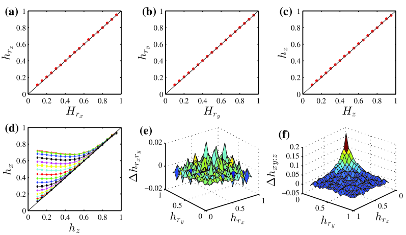
Figure 1: (color online.) Detrended partial cross-correlation exponents. (a-b) Dependence of the average Hurst indices $h_{r_{x}}$ and $h_{r_{x}}$ of the two components of the generated bivariate fractional Brownian motions on the input Hurst indices $H_{r_{x}}$ and $H_{r_{x}}$. (c) Dependence of the average Hurst index $h_{z}$ of the generated univariate fractional Brownian motions on the input Hurst index $H_{z}$. (d) Dependence of $h_{x}$ on $H_{z}$ for different $h_{r_{x}}$ values. (e) Relative error $\Delta{h_{r_{x}r_{y}}}=h_{r_{x}r_{y}}-H_{r_{x}r_{y}}$. (f) Relative error $\Delta{h_{xy:z}}$ between the DPXA estimate $\langle{h_{xy:z}}\rangle_{z}$ and the true value $h_{r_{x}r_{y}}$ as a function of $h_{r_{x}}$ and $h_{r_{y}}$.

We assume that the local trend functions of $R_{x,v}$ and $R_{x,v}$ are $\widetilde{R}_{x,v}$ and $\widetilde{R}_{y,v}$, respectively. The detrended partial cross-correlation in each window is then calculated,

$$F_{v}^{2}(s)=\frac{1}{s}\sum_{k=1}^{s}\left[R_{x,v}(k)-\widetilde{R}_{x,v}(k)\right]\left[R_{y,v}(k)-\widetilde{R}_{y,v}(k)\right],$$ (5)

and the second-order detrended partial cross-correlation is calculated,

$$F_{xy:{\bm{z}}}(2,s)=\left[\frac{1}{m-1}\sum_{v=1}^{m}F_{v}^{2}(s)\right]^{1/2}.$$ (6)

If there are intrinsic long-range power-law cross-correlations between $x$ and $y$, we expect the scaling relation,

$$F_{xy:{\bm{z}}}(2,s)\sim s^{h_{xy:{\bm{z}}}}.$$ (7)

There are many ways of determining $\widetilde{R}_{x,v}$ and $\widetilde{R}_{y,v}$. The local detrending functions could be polynomials Peng et al. (1994); Hu et al. (2001), moving averages Vandewalle and Ausloos (1998); Alessio et al. (2002); Xu et al. (2005); Arianos and Carbone (2007), or other possibilities Qian et al. (2011). To distinguish the different detrending methods, we label the corresponding DPXA variants as, e.g., PX-DFA and PX-DMA. When the moving average is used as the local detrending function, the window size of the moving averages must be the same as the covering window size $s$ Gu and Zhou (2010).

To measure the validity of the DPXA method, we perform numerical experiments using an additive model for $x$ and $y$, i.e.,

$$\left\{\begin{array}[]{ccc}x(t)=\beta_{x,0}+\beta_{x}z(t)+r_{x}(t)\\ y(t)=\beta_{y,0}+\beta_{y}z(t)+r_{y}(t)\end{array}\right.,$$ (8)

where $z(t)$ is a fractional Gaussian noise with Hurst index $H_{z}$, and $r_{x}$ and $r_{y}$ are the incremental series of the two components of a bivariate fractional Brownian motion (BFBMs) with Hurst indices $H_{r_{x}}$ and $H_{r_{y}}$ Lavancier et al. (2009); Coeurjolly et al. (2010); Amblard et al. (2013). The properties of multivariate fractional Brownian motions have been extensively studied Lavancier et al. (2009); Coeurjolly et al. (2010); Amblard et al. (2013). In particular, it has been proven that the Hurst index $H_{r_{x}r_{y}}$ of the cross-correlation between the two components is Lavancier et al. (2009); Coeurjolly et al. (2010); Amblard et al. (2013)

$$H_{r_{x}r_{y}}=(H_{r_{x}}+H_{r_{y}})/2.$$ (9)

This property allows us to assess how the proposed method perform. We can obtain the $h_{xy}$ of $x$ and $y$ using the DCCA method and the $h_{xy:{\bm{z}}}$ of $r_{x}$ and $r_{y}$ using the DPXA method. Our numerical experiments show that $H_{r_{x}r_{y}}=h_{r_{x}r_{y}}=h_{xy:{\bm{z}}}\neq h_{xy}$. We use $H$ for theoretical or true values and $h$ for numerical estimates.

In the simulations we set $\beta_{x,0}=2$, $\beta_{x}=3$, $\beta_{y,0}=2$, and $\beta_{y}=3$ in the model based on Eq. (8). Three Hurst indices $H_{r_{x}}$, $H_{r_{y}}$, and $H_{z}$ are input arguments and vary from 0.1 to 0.95 at 0.05 intervals. Because $r_{x}$ and $r_{y}$ are symmetric, we set $H_{r_{x}}\leq H_{r_{y}}$, resulting in $\frac{(18+1)\times 18}{2}\times 18=3078$ triplets of $(H_{r_{x}},H_{r_{y}},H_{z})$. The BFBMs are simulated using the method described in Ref. Coeurjolly et al. (2010); Amblard et al. (2013), and the FBMs are generated using a rapid wavelet-based approach Abry and Sellan (1996). The length of each time series is 65536. For each $(H_{r_{x}},H_{r_{y}},H_{z})$ triplet we conduct 100 simulations. We obtain the Hurst indices for the simulated time series $r_{x}$, $r_{y}$, $z$, $x$, and $y$ using detrended fluctuation analysis Peng et al. (1994); Kantelhardt et al. (2001). The average values $h_{r_{x}}$, $h_{r_{y}}$, $h_{z}$, $h_{x}$, and $h_{y}$ over 100 realizations are calculated for further analysis, which are shown in Fig. 1. A linear regression between the output and input Hurst indices in Fig. 1(a–c) yields $\langle{h_{r_{x}}}\rangle=0.009+0.990H_{r_{x}}$, $\langle{h_{r_{y}}}\rangle=0.009+0.990H_{r_{y}}$, and $\langle{h_{z}}\rangle=0.010+0.991H_{z}$, suggesting that the generated FBMs have Hurst indices equal to the input Hurst indices. Figure 1(d) shows that when $h_{r_{x}}\leq h_{z}$, $h_{x}$ is close to $h_{z}$. When it is not, $h_{z}<h_{x}<h_{r_{x}}$.

Figure 1(e) shows that $h_{r_{x}r_{y}}=(h_{r_{x}}+h_{r_{y}})/2$. Because $h_{r_{x}}\approx H_{r_{x}}$ and $h_{r_{y}}\approx H_{r_{y}}$ [see Fig. 1(a)–(b)], we verify numerically that

$$h_{r_{x}r_{y}}\approx H_{r_{x}r_{y}}.$$ (10)

Note also that $h_{xy}\approx(h_{x}+h_{y})/2$, and that $h_{xy:z}$ is a function of $h_{r_{x}}$, $h_{r_{y}}$ and $h_{z}$. A simple linear regression gives

$$h_{xy:z}=0.003+0.509h_{r_{x}}+0.493h_{r_{y}}+0.012h_{z},$$ (11)

which indicates that the DPXA method can be used to extract the intrinsic cross-correlations between the two time series $x$ and $y$ when they are influenced by a common factor $z$. We calculate the average $\langle{h_{xy:z}}\rangle_{z}$ over different $H_{z}$ and then find the relative error

$$\Delta{h_{xy:z}}=\frac{\langle{h_{xy:z}}\rangle_{z}-h_{r_{x}r_{y}}}{h_{r_{x}r_{y}}}.$$ (12)

Figure 1(f) shows the results for different combinations of $h_{r_{x}}$ and $h_{r_{y}}$. Although in most cases we see that $\Delta{h_{xy:z}}\ll 0.05$, when both $h_{r_{x}}$ and $h_{r_{y}}$ approach 0, $\Delta{h_{xy:z}}$ increases. When $h_{r_{x}}=h_{r_{y}}=0.11$, $\Delta{h_{xy:z}}=0.192$, and when $h_{r_{x}}=0.11$ and $h_{r_{y}}=0.16$, $\Delta{h_{xy:z}}=0.113$. For all other points of $(h_{r_{x}},h_{r_{y}})$, the relative errors $\Delta{h_{xy:z}}$ are less than 0.10.

II.2 DPXA coefficient

In a way similar to detrended cross-correlation coefficients Zebende (2011); Kristoufek (2014), we define the detrended partial cross-correlation coefficient (or DPXA coefficient) as

$$\rho_{\rm{DPXA}}(s)=\rho_{xy:z}(s)=\frac{F^{2}_{xy:{\bm{z}}}(2,s)}{F_{x:{\bm{z}}}(2,s)F_{y:{\bm{z}}}(2,s)}.$$ (13)

As in the DCCA coefficient Podobnik et al. (2011); Kristoufek (2014), we also find $-1\leq{\rho_{\rm{DPXA}}(s)}\leq 1$ for DPXA. The DPXA coefficient indicates the intrinsic cross-correlations between two non-stationary series.

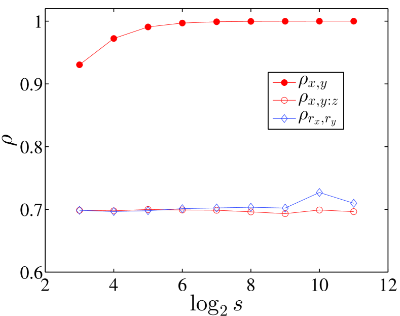
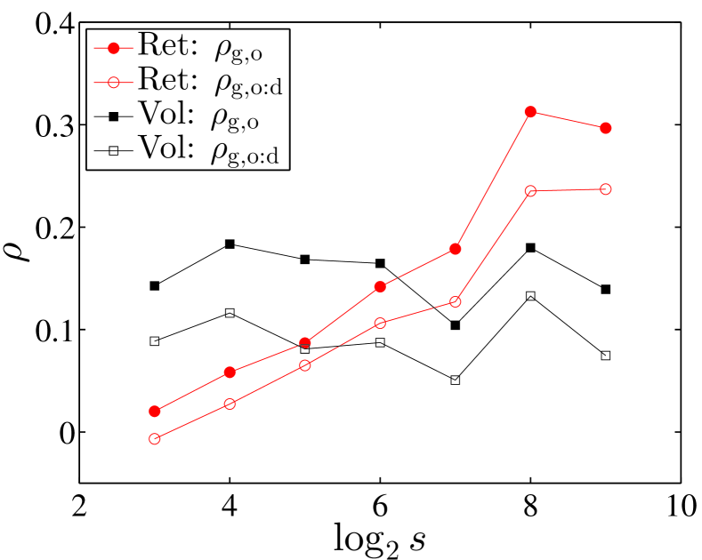
Figure 2: (color online.) Detrended partial cross-correlation coefficients. (a) Performance of different methods by comparing three cross-correlation coefficients $\rho_{x,y}$, $\rho_{r_{x},r_{y}}$ and $\rho_{x,y:z}$ of the mathematical model in Eq. (8). (b) Estimation and comparison of the cross-correlation levels between the two return time series ($\circ$) and two volatility time series ($\square$) of crude oil and gold when including and excluding the influence of the USD index.

We use the mathematical model in Eq. (8) with the coefficients $\beta_{x,0}=\beta_{y,0}=2$ and $\beta_{x,1}=\beta_{y,1}=3$ to demonstrate how the DPXA coefficient outperforms the DCCA coefficient. The two components $r_{x}$ and $r_{y}$ of the BFBM have very small Hurst indices $H_{r_{x}}=0.1=H_{r_{y}}=0.1$ and their correlation coefficient is $\rho=0.7$, and the driving FBM force $z$ has a large Hurst index $H_{z}=0.95$. Figure 2(a) shows the resulting cross-correlation coefficients at different scales. The DCCA coefficients $\rho_{r_{x},r_{y}}$ between the generated $r_{x}$ and $r_{y}$ time series overestimate the true value $\rho=0.7$. Because the influence of $z$ on $r_{x}$ and $r_{y}$ is very strong, the behaviors of $x$ and $y$ are dominated by $z$, and the cross-correlation coefficient $\rho_{x,y}(s)$ is close to 1 when $s$ is small and approaches 1 when $s$ us large. In contrast, the DPXA coefficients $\rho_{x,y:z}$ are in good agreement with the true value $\rho=0.7$. Note that the DPXA method better estimates $r_{x}$ and $r_{y}$ than the DCCA method, since the $\rho_{r_{x},r_{y}}$ curve deviates more from the horizontal line $\rho=0.7$ than the $\rho_{x,y:z}$ curve, especially at large scales.

To illustrate the method with an example from finance, we use it to estimate the intrinsic cross-correlation levels between the futures returns and the volatilities of crude oil and gold. It is well-documented that the returns of crude oil and gold futures are correlated Zhang and Wei (2010), and that both commodities are influenced by the USD index Wang and Chueh (2013). The data samples contain the daily closing prices of gold, crude oil, and the USD index from 4 October 1985 to 31 October 2012. Figure 2(b) shows that both the DCCA and DPXA coefficients of returns exhibit an increasing trend with respect to the scale $s$, and that the two types of coefficient for the volatilities do not exhibit any evident trend. For both financial variables, Fig. 2(b) shows that

$$\rho_{\mathrm{g,o:d}}(s)<\rho_{\mathrm{g,o}}(s)$$ (14)

for different scales. Although this is similar to the result between ordinary partial correlations and cross-correlations Kenett et al. (2015), the DPXA coefficients contain more information than the ordinary partial correlations since the former indicate the partial correlations at multiple scales.

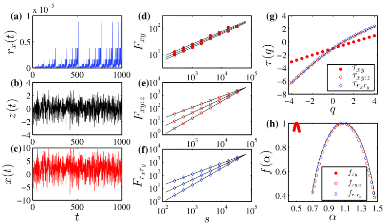
Figure 3: (color online.) Multifractal detrended partial cross-correlation analysis of two binomial measures contaminated by Gaussian noise with very low signal-to-noise ratio. (a-c) The segments of the binomial signal $r_{x}(t)$ with $p_{x}=0.3$, the Gaussian noise $z(t)$, and the “observed” signal $x(t)$. (d-f) Power-law dependence of the fluctuations $F_{xy}(q,s)$, $F_{xy:z}(q,s)$, $F_{r_{x}r_{y}}(q,s)$ on the scale $s$ for $q=-4$, 0 and 4 (top down). The values of $F_{xy:z}$ and $F_{r_{x}r_{y}}$ have been multiplied by $10^{5}$. (g) Multifractal mass exponents $\tau_{xy}(q)$, $\tau_{xy:z}(q)$ and $\tau_{r_{x}r_{y}}(q)$, with the theoretical curve ${\cal{T}}_{r_{x}r_{y}}$ shown as a continuous line. (d) Multifractal spectra $f_{xy}(\alpha)$, $f_{xy:z}(\alpha)$, $f_{r_{x}r_{y}}(\alpha)$ of the singularity strength $\alpha$. The continuous curve is the theoretical spectrum ${\cal{F}}_{r_{x}r_{y}}(\alpha)$.

III Multifractal detrended partial cross-correlation analysis

An extension of the DPXA for multifractal time series, notated MF-DPXA, can be easily implemented. When MF-DPXA is implemented with DFA or DMA, we notate it MF-PX-DFA or MF-PX-DMA. The $q$th order detrended partial cross-correlation is calculated

$$F_{xy:{\bm{z}}}(q,s)=\left[\frac{1}{m-1}\sum_{v=1}^{m}|F_{v}^{2}(s)|^{q/2}\right]^{1/q}$$ (15)

when $q\neq 0$, and

$$F_{xy:{\bm{z}}}(0,s)=\exp\left[\frac{1}{m}\sum_{v=1}^{m}\ln|F_{v}(s)|\right]~{}.$$ (16)

We then expect the scaling relation

$$F_{xy:{\bm{z}}}(q,s)\sim s^{h_{xy:{\bm{z}}}(q)}~{}.$$ (17)

According to the standard multifractal formalism, the multifractal mass exponent $\tau(q)$ can be used to characterize the multifractal nature, i.e.,

$$\tau_{xy:{\bm{z}}}(q)=qh_{xy:{\bm{z}}}(q)-D_{f},$$ (18)

where $D_{f}$ is the fractal dimension of the geometric support of the multifractal measure Kantelhardt et al. (2002). We use $D_{f}=1$ for our time series analysis. If the mass exponent $\tau(q)$ is a nonlinear function of $q$, the signal is multifractal. We use the Legendre transform to obtain the singularity strength function $\alpha(q)$ and the multifractal spectrum $f(\alpha)$ Halsey et al. (1986)

$$\left\{\begin{array}[]{ll}\alpha_{xy:{\bm{z}}}(q)={\rm{d}}\tau_{xy:{\bm{z}}}(q)/{\rm{d}}q\\ f_{xy:{\bm{z}}}(q)=q{\alpha_{xy:{\bm{z}}}}-{\tau_{xy:{\bm{z}}}}(q)\end{array}\right..$$ (19)

To test the performance of MF-DPXA, we construct two binomial measures $\{r_{x}(t):t=1,2,\cdots,2^{k}\}$ and $\{r_{y}(t):t=1,2,\cdots,2^{k}\}$ from the $p$-model with known analytic multifractal properties Meneveau and Sreenivasan (1987), and contaminate them with Gaussian noise. We generate the binomial measure iteratively Jiang and Zhou (2011) by using the multiplicative factors $p_{x}=0.3$ for $r_{x}$ and $p_{y}=0.4$ for $r_{y}$. The contaminated signals are $x=2+3z+r_{x}$ and $y=2+3z+r_{y}$. Figures 3(a)–(c) show that the signal-to-noise ratio is of order $O(10^{-6})$. Figures 3(d)–(f) show a power-law dependence between the fluctuation functions and the scale, in which it is hard to distinguish the three curves of $F_{xy}$. Figure 3(g) shows that for $x(t)$ and $y(t)$, the $\tau_{xy}(q)$ function an approximate straight line and that the corresponding $f_{xy}(\alpha)$ spectrum is very narrow and concentrated around $\alpha=0.5$. These observations are trivial because $x(t)$ and $y(t)$ are Gaussian noise with the Hurst indices $H_{x}=H_{y}=0.5$, and the multifractal detrended cross-correlation analysis Zhou (2008) fails to uncover any multifractality. On the contrary, we find that $\tau_{xy:z}(q)\approx\tau_{r_{x}r_{y}}(q)\approx{\cal{T}}_{r_{x}r_{y}}(q)$ and $f_{xy:z}(\alpha)\approx f_{r_{x}r_{y}}(\alpha)\approx{\cal{F}}_{r_{x}r_{y}}(\alpha)$. Thus the MF-DPXA method successfully reveals the intrinsic multifractal nature between $r_{x}(t)$ and $r_{y}(t)$ hidden in $x(t)$ and $y(t)$.

IV Summary

In summary, we have studied the performances of DPXA exponents, DPXA coefficients, and MF-DPXA using bivariate fractional Brownian motions contaminated by a fractional Brownian motion and multifractal binomial measures contaminated by white noise. These mathematical models are appropriate here because their analytical expressions are known. We have demonstrated that the DPXA methods are capable of extracting the intrinsic cross-correlations between two time series when they are influenced by common factors, while the DCCA methods fail.

The methods discussed are intended for multivariate time series analysis, but they can also be generalized to higher dimensions Gu and Zhou (2006); Carbone (2007); Gu and Zhou (2010); Jiang and Zhou (2011). We can also use lagged cross-correlations in these methods Podobnik et al. (2010); Shen (2015). Although comparing the performances of different methods is always important Shao et al. (2012), different variants of a method can produce different outcomes when applied to different systems. For instance, one variant that outperforms other variants under the setting of certain stochastic processes is not necessary the best performing method for other systems Gu and Zhou (2010). We argue that there are still a lot of open questions for the big family of DFA, DMA, DCCA and DPXA methods.