Microscopic toy model for Cavity dynamical Casimir effect

Abstract

We develop a microscopic toy model for Cavity dynamical Casimir effect (DCE), namely, the photon generation from vacuum due to a nonstationary dielectric slab in a fixed single mode cavity. We represent the slab by $N\gg 1$ noninteracting two-level atoms coupled to the field via the standard dipole interaction. We show that the DCE is contained implicitly in the light–matter interaction Hamiltonian when its parameters are externally prescribed functions of time. We also predict several new phenomena, such as saturation of the photon growth due to effective Kerr nonlinearity, generation of pairs of atomic excitations instead of photons (“Inverse DCE”) and coherent annihilation of pair of system excitations due to the atomic modulation (“Anti-DCE”). These results are extended to the circuit QED architecture, where similar effects can be implemented with a single qubit providing an alternative way to generate cavity and atom–field entangled states.

I Introduction

The term “dynamical Casimir effect” (DCE) is used nowadays for a rather wide group of phenomena characterized by creation of quanta from the initial vacuum state of some field due to time-dependent variations of the geometry or material properties of a macroscopic or mesoscopic system (see book ; vdodonov ; revDal ; nori ; CAMOP-me for recent reviews). In particular, Cavity DCE 2 denotes the process of photon generation from the electromagnetic vacuum (and other initial states) in cavities due to the motion of some wall or the time-modulation of the material properties (e.g., dielectric permittivity or conductivity) of the wall or a medium inside the cavity bound2 ; diss4 . An analog of Cavity DCE was recently implemented experimentally in the solid state architecture known as circuit Quantum Electrodynamics (circuit QED cir1 ; cir2 ; cir3 ), where a Josephson metamaterial was embedded in a low-Q microwave cavity, permitting the modulation of the cavity effective length via external magnetic field meta .

Although Cavity DCE has been studied theoretically for more than four decades, some aspects of this phenomenon are still not completely clear. A particular issue we approach here is the asymptotic behavior of photon generation: while some models predict the saturation of the intra-cavity photon number sat1 ; sat2 , other predict exponential photon growth even in the presence of moderate dissipation diss1 ; diss2 ; diss3 ; diss4 ; diss5 ; diss6 . This controversy can be resolved by constructing a full microscopic model for the interaction between the quantized electromagnetic field and moving or time-modulated objects constituted of individual atoms. Some steps along this line were taken in asym1 ; asym2 , yet the majority of studies employs time-varying boundary conditions for the cavity field to bypass the complicated light–matter interaction at the interface book ; nori ; bound1 ; bound2 ; bound3 ; bound4 ; bound5 ; bound6 ; bound7 .

In this paper we utilize the general mathematical description of nonstationary circuit QED systems formulated recently in JPA to develop a microscopic toy model for Cavity DCE. Our study is motivated by the following intuition: since the boundary conditions are just a mathematical artifact to manage the interaction between photons and a large number of atoms, DCE should ultimately originate from the basic form of light–matter interaction with nonstationary parameters. So we consider the special case of Cavity DCE implemented with a dielectric slab having externally prescribed motion and material properties. The slab is portrayed as an ensemble of $N$ two-level atoms with unspecified transition frequencies and coupling strengths that interact with the field via the standard dipole Hamiltonian with time-dependent parameters schleich . We use the time-independent boundary conditions to quantize the cavity field in a standard manner, while the interaction between the arbitrarily modulated atoms and photons is treated microscopically.

After cumbersome calculations we arrive at simple mathematical expressions that generalize the common DCE description in single-mode cavities bound2 ; zeilinger . In particular, we express the photon generation rate in terms of the microscopic parameters, show that the photon growth and amount of squeezing are limited due to effective Kerr nonlinearity and point out that Cavity DCE occurs even for a single atom. Moreover, we discuss how external classical pumping can significantly enhance the photon generation from vacuum for suitable choices of the pump phase seed . Since our model is quite general, we also apply it to situations where all the system parameters are known, such as a cloud of cold polar molecules polar1 ; polar2 or superconducting qubits cir3 ; cir4 ; cir5 . New effects arising from periodic external modulations are analyzed: generation of pairs of atomic excitations from vacuum (“Inverse DCE”), coherent annihilation of a pair of system excitations (“Anti-DCE”) and generation of entangled light–matter states.

This paper is organized as follows. In section II we formulate our problem and in section III we develop the toy model for cavity DCE, presenting the analytical and numerical results. In section IV we extend our analysis to cold atomic clouds, where all the atomic parameters are known and, in principle, can be modulated externally. In section V we repeat this analysis for the case of a single two-level atom, discussing the Anti-DCE behavior and studying some applications in the area of circuit QED. Section VI contains the conclusions. This paper contains two extensive appendices: in A we give the thorough analytical description for the case $N\gg 1$ in the Heisenberg picture, while in B we do the same for $N=1$ in the Schrödinger picture.

II Mathematical formulation of the problem

We quantize the cavity field using the standard methods with time-independent boundary conditions schleich ; vogel . The annihilation and creation operators $\hat{a}$ and $\hat{a}^{\dagger}$ do not depend explicitly on time, so the vacuum state defined as $\hat{a}|0\rangle=0$ book ; nori is the same for all times, unlike the case of a cavity with moving walls for which the field state depends on the instantaneous frequency diss2 . We consider a small dielectric slab located at an arbitrary position within the cavity, as depicted in figure 1. The dielectric slab is subject to pre-determined motion with small amplitude, and its material properties (e.g., dielectric permittivity) can be adjusted externally by some bias (represented by the laser beam in the figure). From the microscopic point of view, this problem corresponds to a predetermined motion of an atomic cloud whose internal properties are modulated externally. For consistency, the generation of photons from vacuum in this particular example of DCE should be contained intrinsically within any formulation of the light–matter interaction.

Figure 1: Artistic view of DCE due to a nonstationary dielectric slab in a fixed single-mode cavity. The dielectric slab (pictured as a set of $N$ noninteracting Hydrogen atoms) oscillates according to an external law of motion, while its dielectric properties can be modulated externally via electric or magnetic fields. The harmonic wave represents the time-independent cavity mode function; red beam represents the modulation of the material properties of the dielectric. The zoom shows an individual atom containing one proton and one electron, whose center-of-mass coordinate $\mathbf{R}$ changes due to the prescribed motion.

We consider the simplest microscopic model for the dielectric slab – a set of $N$ non-interacting Hydrogen atoms, as shown in the zoom of figure 1. First we recapitulate the interaction of a single atom with the field. Each atom consists of a proton (electron), described by the position operator $\mathbf{\hat{r}}_{p}$ ($\mathbf{\hat{r}}_{e}$), with mass $m_{p}$ ($m_{e}$) and charge $e$ ($-e$). Introducing the center-of-mass (CM) position operator $\mathbf{\hat{R}}=(m_{e}\mathbf{\hat{r}}_{e}+m_{p}\mathbf{\hat{r}}_{p})/M$, where $M=m_{e}+m_{p}$ is the total atomic mass, we define the momentum operator $\mathbf{\hat{P}=\hat{p}}_{e}+\mathbf{\hat{p}}_{p}$ associated with the CM motion, where $\mathbf{\hat{p}}_{p}$ ($\mathbf{\hat{p}}_{e}$) is the canonical momentum operator of the proton (electron). Furthermore, one introduces the relative coordinate between the proton and electron $\mathbf{\hat{r}}=\mathbf{\hat{r}}_{e}-\mathbf{\hat{r}}_{p}$ and the momentum $\mathbf{\hat{p}}=(m_{p}\mathbf{\hat{p}}_{e}+m_{e}\mathbf{\hat{p}}_{p})/M$ associated with the relative motion of the reduced mass $\mu=m_{e}m_{p}/M$. As a result, we can decompose the dynamics into the motion of CM and the relative motion, with the total kinetic energy given by $\mathbf{\hat{p}}_{e}^{2}/(2m_{e})+\mathbf{\hat{p}}_{p}^{2}/(2m_{p})=\mathbf{\hat{P}}^{2}/(2M)+\mathbf{\hat{p}}^{2}/(2\mu)$.

We treat the light–matter interaction in the first-order dipole approximation, assuming that the dimensions of the atom are much smaller than the wavelength of the cavity mode. The minimal coupling Hamiltonian in the Coulomb gauge is minutely deduced in schleich . Considering that the CM motion is prescribed externally, with $\mathbf{P}$ and $\mathbf{R}$ given by known functions of time, it reads

$$\hat{H}^{(1)} = \frac{\mathbf{P}^{2}}{2M}+\hat{H}_{f}+\hat{H}_{a}-e\mathbf{\hat{r}}\cdot\left[\mathbf{\hat{E}}+\mathbf{\dot{R}}\times\mathbf{\hat{B}}\right]+e^{2}\left(\frac{1}{8\mu}-\frac{1}{M}\right)\left[\mathbf{\hat{r}}^{2}\mathbf{\hat{B}}^{2}-(\mathbf{\hat{r}}\cdot\mathbf{\hat{B})}^{2}\right]$$ (1)

$$-\frac{e(m_{p}-m_{e})}{2M}\left[\frac{1}{\mu}\,\mathbf{\hat{B}}\cdot(\mathbf{\hat{r}}\times\mathbf{\hat{p})}+(\mathbf{\hat{r}}\cdot\mathbf{\nabla}_{\mathbf{R}})\mathbf{\hat{r}}\cdot\mathbf{\hat{E}}\right]~{}.$$

Here $\hat{H}_{f}=\hbar\omega\hat{n}$ is the cavity free Hamiltonian, where $\omega$ is the frequency and $\hat{n}=\hat{a}^{\dagger}\hat{a}$ is the photon number operator. $\hat{H}_{a}=\mathbf{\hat{p}}^{2}/(2\mu)+V(\mathbf{\hat{r})}$ is the Hamiltonian of the atomic internal dynamics, where $V(\mathbf{\hat{r})}=-e^{2}/(4\pi\varepsilon_{0}|\mathbf{\hat{r}|})$ is the Coulomb interaction energy and $\varepsilon_{0}$ is the permittivity of vacuum. The electric and magnetic intracavity fields are

$$\mathbf{\hat{E}}\left(\mathbf{R}\right)=i\sqrt{\frac{\hbar\omega}{2\varepsilon_{0}V}}\mathbf{u}\left(\mathbf{R}\right)\left(\hat{a}-\hat{a}^{\dagger}\right)~{}$$ (2)

$$\mathbf{\hat{B}}\left(\mathbf{R}\right)=\sqrt{\frac{\hbar}{2\varepsilon_{0}V\omega}}\left(\mathbf{\nabla}\times\mathbf{u}\left(\mathbf{R}\right)\right)\left(\hat{a}+\hat{a}^{\dagger}\right)\,,$$ (3)

where $V$ is the mode volume and $\mathbf{u}\left(\mathbf{R}\right)$ is the dimensionless mode function determined from the time-independent boundary conditions on the walls. In the stationary case, when $\mathbf{\dot{R}=0}$, one usually neglects the contributions containing the magnetic field and the gradient of the electric field in Hamiltonian (1), recovering the standard dipole interaction term $-e\mathbf{\hat{r}}\cdot\mathbf{\hat{E}}$. However, in the nonstationary regime $\mathbf{\dot{R}\neq 0}$ all the terms must be taken into account schleich .

For our toy model we take into consideration only the two atomic levels near-resonant with the cavity frequency, restricting the atomic dynamics to the “ground” and “excited” states $|g\rangle$ and $|e\rangle$, respectively. Hence the atomic Hamiltonian reads $\hat{H}_{a}=\hbar\Omega\hat{\sigma}_{z}/2$, where $\Omega$ is the transition frequency and $\hat{\sigma}_{z}=|e\rangle\langle e|-|g\rangle\langle g|$ is the Pauli operator. For the two-level approximation to hold we must have $|\omega-\Omega|\ll\omega$. The position operator can be written as $\mathbf{\hat{r}=r}_{0}\hat{\sigma}_{+}+\mathbf{r}_{0}^{\ast}\hat{\sigma}_{-}$, where $\mathbf{r}_{0}=\langle e|\mathbf{\hat{r}}|g\rangle$ is the off-diagonal matrix element and the Pauli ladder operators are $\hat{\sigma}_{+}=|e\rangle\langle g|$ and $\hat{\sigma}_{-}=|g\rangle\langle e|$. In this case $\mathbf{\hat{r}}^{2}=|\mathbf{r}_{0}|^{2}$ and the square of the magnetic field operator $\propto(\hat{a}+\hat{a}^{\dagger})^{2}$ appears naturally in Hamiltonian (1).

Hence the simplest model for a nonstationary dielectric slab in a stationary cavity is described by the general Hamiltonian of the form (we set $\hbar=1$)

$$\hat{H}=\omega\hat{n}+\sum_{l=1}^{N}\left[\frac{\Omega}{2}\hat{\sigma}_{z}^{(l)}+g(\hat{a}+\hat{a}^{\dagger})(\hat{\sigma}_{+}^{(l)}+\hat{\sigma}_{-}^{(l)})\right]+i\chi(\hat{a}^{\dagger 2}-\hat{a}^{2})+id(\hat{a}^{\dagger}-\hat{a})~{},$$ (4)

where the index $l$ labels the identical noninteracting atoms. The renormalized cavity frequency $\omega$ is constant, while the atomic transition frequency $\Omega$, the atom–cavity coupling strength$~{}g$ and the “squeezing coefficient” $\chi$ are regarded as externally prescribed functions of time. This occurs both due to the motion of the slab and the external in situ modulation of the atomic properties, though here we do not pursue the exact dependence. The last term on the right-hand side (RHS) of equation (4) accounts for the classical one-photon pumping of the cavity field cir1 , included for generality and to study how DCE can be enhanced by an additional coherent drive.

To understand the emergence of DCE from the microscopic viewpoint we do not need to know the exact relation between the parameters of Hamiltonians (1) and (4), since for a weak external perturbation of the system we can write

$$X=X_{0}+\varepsilon_{X}\sum_{j}w_{X}^{(j)}\sin\left(\eta^{(j)}t+\varphi_{X}^{(j)}\right)~{},~{}X=\{\omega,\Omega,g,\chi,d\}\,,$$ (5)

where $X_{0}$ is the bare value and $\varepsilon_{X}\geq 0$ is the modulation depth of $X$. The sum runs over all the present modulation frequencies $\eta^{(j)}$; we can write it as $\sum_{j}=\sum_{j}^{\prime}+\sum_{j}^{\prime\prime}$, where $\sum_{j}^{\prime}$ denotes the sum over “fast” modulation frequencies, $\eta^{(j\prime)}\gtrsim\omega_{0}$, and $\sum_{j}^{\prime\prime}$ – over “slow” modulation frequencies, $\eta^{(j\prime\prime)}\ll\omega_{0}$. Parameters $w_{X}^{(j)}\geq 0$ and $\varphi_{X}^{(j)}$ are the relative weights and phase constants corresponding to the modulation of $X$ at frequency $\eta^{(j)}$. For the classical pump we set $d_{0}=0$, and we included the modulation of $\omega$ in equation (5) for the sake of generality. For the future use we define the complex modulation depth $\varepsilon_{X}^{(j)}$ that includes the weight and the phase of $X$-modulation at frequency $\eta^{(j)}$

$$\varepsilon_{X}^{(j)}\equiv\varepsilon_{X}w_{X}^{(j)}\exp[i\phi_{X}^{(j)}]~{},~{}X=\{\omega,\Omega,g,\chi,d\}~{}.$$ (6)

Throughout the paper the notation $\varepsilon_{X}^{(j\prime)}$ and $\varepsilon_{X}^{(j\prime\prime)}$ stands for the complex modulation depths corresponding to fast and slow modulation frequencies, respectively.

III Toy model for DCE with a dielectric slab

As a toy model for DCE we consider a fixed cavity of known frequency $\omega_{0}$ that contains $N$ identical two-level atoms. The atomic transition frequency $\Omega$ and the coupling strength $g$ are unknown, but in order to represent the dielectric slab the difference $\omega_{0}-\Omega$ must be large compared to the coupling strength, $|\omega_{0}-\Omega|\gg|g|$. Due to the external perturbation the parameters $\Omega$, $g$ and $\chi$ vary according to equation (5), and we consider the general case when the three parameters can change simultaneously. For the macroscopic slab we consider $N\gg 1$ and define the collective operators via the Holstein–Primakoff transformation HP

$$\sum_{l=1}^{N}\hat{\sigma}_{+}^{(l)}=\hat{b}^{\dagger}(N-\hat{b}^{\dagger}\hat{b})^{1/2}~{}~{},~{}\sum_{l=1}^{N}\hat{\sigma}_{-}^{(l)}=(N-\hat{b}^{\dagger}\hat{b})^{1/2}\hat{b}~{},~{}\sum_{l=1}^{N}\hat{\sigma}_{z}^{(l)}=2\hat{b}^{\dagger}\hat{b}-N~{},$$ (7)

where the ladder operators $\hat{b}$ and $\hat{b}^{\dagger}$ satisfy the bosonic commutation relation $[\hat{b},\hat{b}^{\dagger}]=1$. To the first order in $\hat{b}^{\dagger}\hat{b}/N$ the Hamiltonian for our toy model reads

$$\hat{H}=\omega_{0}\hat{n}+\Omega\hat{b}^{\dagger}\hat{b}+\tilde{g}(\hat{a}+\hat{a}^{\dagger})(\hat{b}+\hat{b}^{\dagger})+i\chi(\hat{a}^{\dagger 2}-\hat{a}^{2})-\frac{\tilde{g}}{2N}(\hat{a}+\hat{a}^{\dagger})(\hat{b}^{\dagger 2}\hat{b}+\hat{b}^{\dagger}\hat{b}^{2})~{},$$ (8)

where we defined the collective coupling constant $\tilde{g}\equiv\sqrt{N}g$, so that $\tilde{g}_{0}=\sqrt{N}g_{0}$ and $\tilde{\varepsilon}_{g}=\sqrt{N}\varepsilon_{g}$ (we consider $g_{0}\geq 0$ without loss of generality). In this paper the tilde over a c-number corresponds to the collective $N$-atoms parameter. The Hamiltonian (8) holds provided the inequality $\langle\hat{b}^{\dagger}\hat{b}\rangle\ll N$ is satisfied.

In the dispersive regime, $|\Delta_{-}|/2\gg\tilde{g}_{0}$, where $\Delta_{-}=\omega_{0}-\Omega_{0}$ is the bare atom–field detuning, the approximate solution in the Heisenberg picture is deduced in A.2:

$$\hat{a} \simeq e^{-i(\omega_{0}-\tilde{\delta}_{+}-\delta_{\chi})t}\left[\hat{A}-i\hat{B}\frac{2\tilde{g}_{0}}{\Delta_{-}}e^{i(\Delta_{-}/2-\delta_{\chi})t}\sin\left(\frac{\Delta_{-}t}{2}\right)\right]$$ (9)

$$\hat{b} \simeq e^{-i(\Omega_{0}-\tilde{\delta}_{+})t}\left[\hat{B}-i\hat{A}\frac{2\tilde{g}_{0}}{\Delta_{-}}e^{-i(\Delta_{-}/2-\delta_{\chi})t}\sin\left(\frac{\Delta_{-}t}{2}\right)\right]$$ (10)

$$\Delta_{+}=\omega_{0}+\Omega_{0}~{},~{}\tilde{\delta}_{\pm}=\frac{\tilde{g}_{0}^{2}}{\omega_{0}\pm\Omega_{0}}~{},~{}\delta_{\chi}=\frac{4\chi_{0}^{2}}{\omega_{0}+\Omega_{0}}~{}.$$ (11)

$\hat{A}$ and $\hat{B}$ are independent bosonic ladder operators that obey the Heisenberg equation of motion $id\hat{O}/dt=[\hat{O},\hat{H}_{eff}]$ ($\hat{O}=\hat{A},\hat{B}$) with the effective Hamiltonian

$$\hat{H}_{eff}=\hat{H}_{G}+\hat{H}_{NG}~{}.$$ (12)

Here $\hat{H}_{G}$ contains the Gaussian part (quadratic terms in the operators $\hat{A}$ and $\hat{B}$) and $\hat{H}_{NG}$ contains the non-Gaussian part (quartic terms).

For the modulation frequency

$$\eta^{(D)}=2(\omega_{0}+\tilde{\delta}_{-}-\tilde{\delta}_{+}-\delta_{\chi}-\zeta)~{},$$ (13)

where we introduced the small adjustable “resonance shift” $\zeta$ in order to perform the fine tuning of the modulation frequency, we find

$$\hat{H}_{G}=qe^{-2it\zeta}\left[\hat{A}^{2}+2e^{-it\delta_{\chi}}\frac{\tilde{g}_{0}}{\Delta_{-}}\hat{A}\hat{B}+e^{-2it\delta_{\chi}}\left(\frac{\tilde{g}_{0}}{\Delta_{-}}\right)^{2}\hat{B}^{2}\right]+h.c.$$ (14)

$$q=\frac{i\tilde{\delta}_{-}\Omega_{0}}{\left(\omega_{0}+\Omega_{0}\right)}\left[\frac{\varepsilon_{\Omega}^{(D)}}{2\Omega_{0}}-\frac{\tilde{\varepsilon}_{g}^{(D)}}{\tilde{g}_{0}}\right]-\frac{\varepsilon_{\chi}^{(D)}}{2}$$ (15)

$$\hat{H}_{NG} = -\frac{\tilde{\delta}_{-}}{2N}\left[\frac{3\tilde{g}_{0}^{2}}{\Delta_{-}^{2}}\hat{A}^{\dagger 2}\hat{A}^{2}-\hat{B}^{\dagger 2}\hat{B}^{2}+\frac{8\tilde{g}_{0}}{\Delta_{-}}\hat{A}\hat{B}^{\dagger 2}\hat{B}e^{i\delta_{\chi}t}+2\hat{A}^{\dagger}\hat{A}\hat{B}^{\dagger}\hat{B}\right.$$

$$\left.-\frac{6\tilde{g}_{0}^{2}}{\Delta_{-}^{2}}\hat{A}^{\dagger 2}\hat{B}^{2}e^{-2i\delta_{\chi}t}-\frac{4\tilde{g}_{0}}{\Delta_{-}}\hat{A}^{\dagger 2}\hat{A}\hat{B}e^{-i\delta_{\chi}t}\right]+i\frac{\tilde{\delta}_{-}}{2N}\frac{\tilde{\varepsilon}_{g}^{(D)}}{\tilde{g}_{0}}e^{-2i\zeta t}\left[\hat{A}^{2}\hat{B}^{\dagger}\hat{B}\right.$$

$$+\frac{3\tilde{g}_{0}^{2}}{2\Delta_{-}^{2}}\hat{A}^{\dagger}\hat{A}^{3}+\frac{2\tilde{g}_{0}}{\Delta_{-}}\hat{A}\hat{B}^{\dagger}\hat{B}^{2}e^{-i\delta_{\chi}t}-\frac{\tilde{g}_{0}}{\Delta_{-}}\hat{A}^{\dagger}\hat{A}^{2}\hat{B}e^{-i\delta_{\chi}t}-\frac{\tilde{g}_{0}}{\Delta_{-}}\hat{A}^{3}\hat{B}^{\dagger}e^{i\delta_{\chi}t}$$

$$-\frac{2\tilde{g}_{0}^{2}}{\Delta_{-}^{2}}\hat{A}^{\dagger}\hat{A}\hat{B}^{2}e^{-2i\delta_{\chi}t}\left.+\frac{\tilde{g}_{0}^{2}}{\Delta_{-}^{2}}\hat{B}^{\dagger}\hat{B}^{3}e^{-2i\delta_{\chi}t}-\frac{\tilde{g}_{0}^{3}}{\Delta_{-}^{3}}\hat{A}^{\dagger}\hat{B}^{3}e^{-3i\delta_{\chi}t}\right]+h.c.$$

These results were obtained under a series of approximations. First, the detuning and the modulation depth of the atomic transition frequency must be small, $\varepsilon_{\Omega},|\Delta_{-}|\ll\omega_{0}$, while the modulation depth of the atom-field coupling strength is $\tilde{\varepsilon}_{g}\lesssim\tilde{g}_{0}$. Second, there are some restraints on the number of excitations in the atoms–field system for which our approach is accurate:

$$\frac{\langle\hat{b}^{\dagger}\hat{b}\rangle}{N},\sqrt{\langle\hat{a}^{\dagger}\hat{a}\rangle+\langle\hat{b}^{\dagger}\hat{b}\rangle}\left\{\frac{\tilde{g}_{0}}{\omega_{0}},\frac{\tilde{\varepsilon}_{g}}{\Delta_{-}},\frac{|\chi_{0}|}{\omega_{0}},\frac{\varepsilon_{\chi}}{\omega_{0}},\frac{\tilde{g}_{0}\varepsilon_{\Omega}}{\Delta_{-}\omega_{0}},\frac{\tilde{g}_{0}\varepsilon_{\chi}}{\Delta_{-}^{2}}\right\}\ll 1$$ (17)

$$\frac{\tilde{g}_{0}}{\Delta_{-}}\sqrt{\langle\hat{a}^{\dagger}\hat{a}\rangle+\langle\hat{b}^{\dagger}\hat{b}\rangle}\left\{\frac{\langle\hat{b}^{\dagger}\hat{b}\rangle}{N},\frac{\sqrt{\langle\hat{b}^{\dagger}\hat{b}\rangle\langle\hat{a}^{\dagger}\hat{a}\rangle}}{N},\frac{\tilde{g}_{0}}{|\Delta_{-}|}\frac{\langle\hat{a}^{\dagger}\hat{a}\rangle}{N}\right\}\ll 1~{}.$$ (18)

Third, in equation (13) there are small “Systematic error frequency shifts” (SEFS) $\Delta\eta$ that were neglected in order to keep the formulae concise. They are of the order

$$O(\Delta\eta) \sim \left\{\tilde{\delta}_{-}\left(\frac{\varepsilon_{\Omega}}{\omega_{0}}\right)^{2},\tilde{\delta}_{-}\left(\frac{\tilde{\varepsilon}_{g}}{\tilde{g}_{0}}\right)^{2},\tilde{\delta}_{-}\left(\frac{\varepsilon_{\chi}}{\Delta_{-}}\right)^{2},\right.$$ (19)

$$\left.\quad\tilde{\delta}_{+}\left(\frac{\varepsilon_{\Omega}}{\Delta_{-}}\right)^{2},\tilde{\delta}_{+}\left(\frac{\Delta_{-}}{\omega_{0}}\right)^{2},\frac{\varepsilon_{\chi}^{2}}{\omega_{0}},\frac{\chi_{0}^{2}}{\omega_{0}}\left(\frac{\Delta_{-}}{\omega_{0}}\right)^{2}\right\}.$$

Hence in the actual implementation of DCE one has to find experimentally the exact modulation frequency by scanning within the range $\Delta\eta$, so in part we introduced the adjustable resonance shift $\zeta$ to achieve this fine tuning.

One can simplify the Hamiltonian (12) a little further. Neglecting the non-Gaussian terms we have

$$\frac{d}{dt}\hat{B}=e^{it\delta_{\chi}}\frac{\tilde{g}_{0}}{\Delta_{-}}\frac{d}{dt}\hat{A}~{},$$ (20)

so for $|q|\gg|\delta_{\chi}|$ we can write

$$\hat{B}(t)\simeq\hat{B}(0)+e^{it\delta_{\chi}}\frac{\tilde{g}_{0}}{\Delta_{-}}\left[\hat{A}(t)-\hat{A}(0)\right]~{}.$$ (21)

Assuming that the cavity and the atoms were initially in the ground states and substituting equation (21) into (12), to the lowest order in $\tilde{g}_{0}/\Delta_{-}$ we obtain the Hamiltonian

$$\hat{H}_{eff}\simeq\left(qe^{-2it\zeta}\hat{A}^{2}+h.c.\right)-N\alpha\left[(\hat{A}^{\dagger}\hat{A})^{2}+\hat{A}^{\dagger}\hat{A}\right]~{},$$ (22)

where

$$\alpha=\frac{g_{0}^{4}}{\Delta_{-}^{3}}$$ (23)

is the effective Kerr nonlinearity strength due to a single two-level atom. Defining the phase $\phi_{q}$ via the relation $q=i\left|q\right|e^{i\phi_{q}}$ and introducing the new annihilation operator

$$\hat{a}_{r}=-ie^{i\phi_{q}/2}e^{-it\zeta}\hat{A}$$ (24)

(that also satisfies $[\hat{a}_{r},\hat{a}_{r}^{\dagger}]=1$), the evolution of $\hat{a}_{r}$ is governed by the time-independent Nonlinear DCE Hamiltonian

$$\hat{H}_{DCE}=\omega_{r}\hat{n}_{r}+\alpha_{r}\hat{n}_{r}^{2}+iq_{r}(\hat{a}_{r}^{\dagger 2}-\hat{a}_{r}^{2})~{}.$$ (25)

Here $\hat{n}_{r}=\hat{a}_{r}^{\dagger}\hat{a}_{r}$, $\omega_{r}=\left(\zeta-N\alpha\right)$,$~{}\alpha_{r}=-N\alpha$ and $q_{r}=\left|q\right|$. The term $iq_{r}(\hat{a}_{r}^{\dagger 2}-\hat{a}_{r}^{2})$, which describes the simplest case of DCE in oscillating cavities bound2 , appears naturally in our derivation. The Hamiltonian (25) is well known from Nonlinear Quantum Optics for describing (in the interaction picture) a cavity that contains a Kerr medium and is parametrically driven kerr1 ; milburn1 ; milburn2 ; kerr2 ; milburn3 ; milburn4 ; milburn5 ; kryuch2 ; kryuch1 ; leonski ; kerr3 ; kryuch3 , so we call $\omega_{r}$ “effective detuning”.

Hence we were able to deduce microscopically the DCE from the most basic form of light–matter interaction, equation (8). It turns out that DCE is described by the cumbersome non-Gaussian Hamiltonian given by equations (14) – (III), and the standard expression for cavity DCE is recovered only to the lowest order in $\tilde{g}_{0}/\Delta_{-}$. Recalling that the auxiliary annihilation operators $\hat{A}$ and $\hat{B}$ are related to the physical annihilation operators $\hat{a}$ and $\hat{b}$ via relations (9) – (10), we can formulate the first new prediction of our toy model: the photon creation from vacuum is accompanied by the excitation of the internal degrees of freedom of the atoms in the slab, which becomes entangled with the cavity field. As stated previously, we assume that the CM motion of the atoms is prescribed externally, so our model does not contemplate the important back-action effects of DCE on the motion of the slab revDal ; back1 ; back2 .

The simplest realistic description of Cavity DCE must include (at least) the Kerr nonlinearity, as shown by equation (25). Although separately the DCE and Kerr Hamiltonians can be integrated in a straightforward manner kerr1 , the general analytical solution for the nonlinear DCE Hamiltonian is not known. To get qualitative insights about the asymptotic dynamics of Hamiltonian (25) we rewrite it in the form of interaction picture parametric amplifier $\hat{H}_{DCE}=\hat{D}_{r}\hat{n}_{r}+iq_{r}(\hat{a}_{r}^{\dagger 2}-\hat{a}_{r}^{2})$, where the overall detuning operator is $\hat{D}_{r}\equiv\omega_{r}+\alpha_{r}\hat{n}_{r}$. Treating the detuning as a c-number $\langle\hat{D}_{r}\rangle$, the solution in the Heisenberg picture reads puri

$$\hat{a}_{r}\left(t\right)=\mathcal{F}^{\ast}\hat{a}_{r}\left(0\right)+\mathcal{G}\hat{a}_{r}^{\dagger}\left(0\right)$$ (26)

$$\mathcal{F}\equiv\cosh\left(\mathcal{B}t\right)+i\frac{\langle\hat{D}_{r}\rangle}{\mathcal{B}}\sinh\left(\mathcal{B}t\right)~{},~{}\mathcal{G}\equiv 2\frac{q_{r}}{\mathcal{B}}\sinh\left(\mathcal{B}t\right)~{},~{}~{}\mathcal{B}=\sqrt{4q_{r}^{2}-\langle\hat{D}_{r}\rangle^{2}}~{}.$$ (27)

So we arrive at the second new prediction of our model: asymptotic exponential photon growth is impossible for nonzero $\alpha_{r}$, as for any fixed value of $\omega_{r}$ the parameter $\mathcal{B}$ becomes imaginary for $\langle\hat{n}_{r}\rangle\rightarrow\infty$. This results solves the controversy about the long-time behavior of Cavity DCE, supporting the finding sat1 ; sat2 that the photon generation is limited even in the absence of dissipation.

To elucidate the system behavior for finite $\langle\hat{n}_{r}\rangle$ we write the wavefunction corresponding to the Hamiltonian $\hat{H}_{DCE}$ as

$$|\psi\rangle=\sum_{m=0}^{\infty}\exp[-it(\omega_{r}m+\alpha_{r}m^{2})]c_{m}|m\rangle~{},$$ (28)

where $|m\rangle$ denotes the Fock state. The probability amplitudes obey the differential equation

$$\dot{c}_{m}=q_{r}[\sqrt{m(m-1)}e^{2it[\omega_{r}+2\alpha_{r}(m-1)]}c_{m-2}-\sqrt{(m+1)(m+2)}e^{-2it[\omega_{r}+2\alpha_{r}(m+1)]}c_{m+2}].$$ (29)

One can easily solve the pair of equations connecting just the amplitudes $c_{K}\left(t\right)$ and $c_{K+2}\left(t\right)$ JPA . For $c_{K+2}\left(0\right)=0$ we get

$$c_{K+2}(t)=e^{it\left[\omega_{r}+2\alpha_{r}\left(K+1\right)\right]}\frac{q_{r}\sqrt{\left(K+1\right)\left(K+2\right)}}{R_{K}}\sin\left(R_{K}t\right)c_{K}(0)~{}$$ (30)

$$R_{K}=\sqrt{[\omega_{r}+2\alpha_{r}(K+1)]^{2}+q_{r}^{2}(K+1)(K+2)}~{}.$$ (31)

So the probability amplitude $c_{K+2}$ is approximately decoupled form $c_{K}$ when $q_{r}\sqrt{(K+1)(K+2)}\ll R_{K}$. For $2|\alpha_{r}|\left(K+1\right)\gg|\omega_{r}|$ the decoupling condition becomes $q_{r}\ll 2|\alpha_{r}|$. Therefore, in order to generate many photons from vacuum one must satisfy the condition $q_{r}\gg 2|\alpha_{r}|$. In the opposite case, $q_{r}\lesssim|\alpha_{r}|$, we expect generation of a small number of photons leonski . For example, for $K=0$ and $q_{r}/|\alpha_{r}|\ll 1$, the effective detuning must be adjusted to $\omega_{r}=-2\alpha_{r}$ to optimize the coupling between the probability amplitudes $c_{0}$ and $c_{2}$. As $q_{r}/|\alpha_{r}|$ increases one can set $\omega_{r}=-2\left(K+1\right)\alpha_{r}$ to optimize the coupling between the amplitudes $\{c_{K},c_{K+2}\}$ ($K=2,4,\ldots$), while the off-resonant coupling between $\{c_{0},c_{2},\cdots,c_{K}\}$ still allows a substantial population of $c_{K}$ 1 . So the question of utmost practical interest is: what value of $\omega_{r}$, or equivalently, what value of the adjustable resonance shift $\zeta$ optimizes the photon generation from vacuum in the presence of Kerr nonlinearity? The answer will given in the next subsection with the help of numerical simulations.

III.1 Numerical results

We studied numerically how the Kerr nonlinearity affects the photon generation from vacuum. For the sake of completeness we included the cavity damping by means of the standard master equation at zero temperature schleich ; vogel

$$\frac{d{\hat{\rho}}}{dt}=-i[\hat{H}_{DCE},\hat{\rho}]+\frac{\kappa}{2}\left(2\hat{a}_{r}\hat{\rho}\hat{a}_{r}^{\dagger}-\hat{a}_{r}^{\dagger}\hat{a}_{r}\hat{\rho}-\hat{\rho}\hat{a}_{r}^{\dagger}\hat{a}_{r}\right),$$ (32)

where $\hat{\rho}$ is the density operator, $\kappa$ is the cavity damping rate and $\hat{H}_{DCE}$ is given by equation (25). Strictly speaking, the microscopic derivation of this master equation does not contemplate the nonstationary case studied here, when the system parameters vary rapidly with time and the counter-rotating terms play a fundamental role bea . Hence the solution of the master equation can only be used to grasp qualitatively the overall effect of dissipation. The stationary state of equation (32) can be calculated analytically using the method of potential solutions for the corresponding Fokker-Planck equation kryuch1 ; kryuch2 . However, as shown in figure 2, the asymptotic solution is of little help for our problem because the cavity field state during the time period of interest (initial times) may be very different from the asymptotic one.

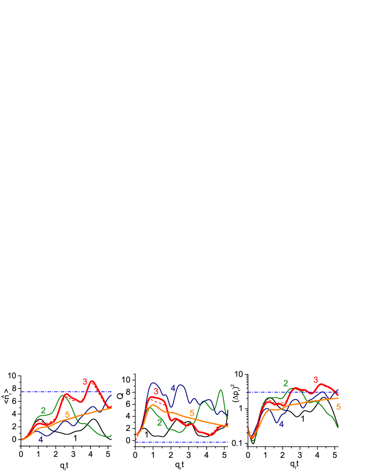
Figure 2: Time behavior of the average photon number $\left\langle\hat{n}_{r}\right\rangle$, Mandel $Q$-factor and the variance of the squeezed quadrature $\left(\Delta p_{r}\right)^{2}$ obtained via numerical integration of equation (32) for $q_{r}=3|\alpha_{r}|$. For curves 1 – 5 the initial state is the vacuum state. For $\kappa=0$ the curves are: $\omega_{r}=0$ (1), $\omega_{r}=-8\alpha_{r}$ (2), $\omega_{r}=-10\alpha_{r}$ (3) and $\omega_{r}=-12\alpha_{r}$ (4). Line 5: $\omega_{r}=-10\alpha_{r}$ and $\kappa=q_{r}$; the dot-dashed line indicates the asymptotic value in this case. The dashed line corresponds to the initial thermal state with the average photon number $\bar{n}=0.1$ and parameters $\omega_{r}=-10\alpha_{r}$, $\kappa=0$.

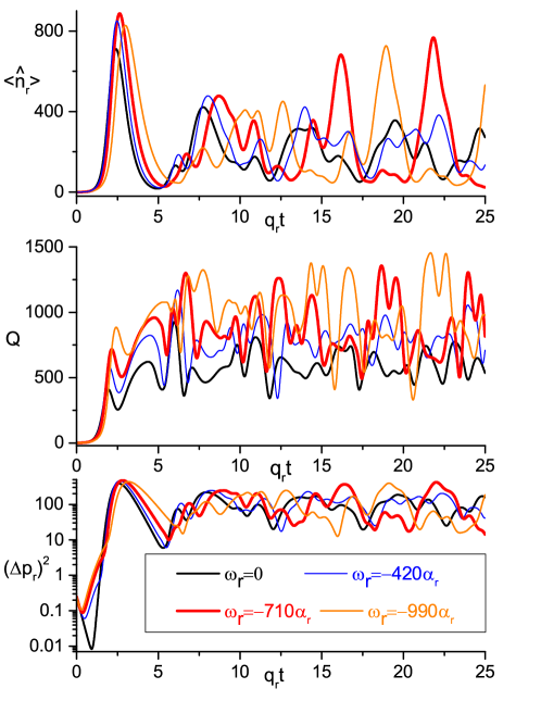
Figure 3: Time behavior of $\left\langle\hat{n}_{r}\right\rangle$, $Q$ and $\left(\Delta p_{r}\right)^{2}$ for the initial vacuum state, $q_{r}=650|\alpha_{r}|$, $\kappa=0$ and different values of $\omega_{r}$. Notice the irregular collapse-revival behavior of $\left\langle\hat{n}_{r}\right\rangle$ and the maximization of the average number of created photons for $\omega_{r}^{(\max)}=-710\alpha_{r}$.

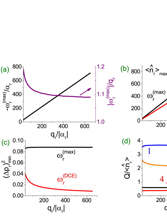
Figure 4: a) Behavior of the effective frequency $\omega_{r}^{(\max)}$ (that maximizes $\langle\hat{n}_{r}\rangle$) as function of $q_{r}/|\alpha_{r}|$. b) Behavior of $\left\langle\hat{n}_{r}\right\rangle_{\max}$ as function of $q_{r}/|\alpha_{r}|$ for the effective frequencies $\omega_{r}^{(\max)}$ and $\omega_{r}^{(\mathrm{DCE})}\equiv 0$. c) Behavior of $\left(\Delta p_{r}\right)_{\min}^{2}$ for these effective frequencies. d) Behavior of $Q/\left\langle\hat{n}_{r}\right\rangle$ at different time instants. Curve 1 (2): $\omega_{r}=\omega_{r}^{(\max)}$ ($\omega_{r}^{(\mathrm{DCE})}$) and the time instant of the minimum value $\left(\Delta p_{r}\right)^{2}$. Curve 3 (4): $\omega_{r}=\omega_{r}^{(\max)}$ ($\omega_{r}^{(\mathrm{DCE})}$) and the time instant of the maximum value of $\left\langle\hat{n}_{r}\right\rangle$.

For small ratio $q_{r}/|\alpha_{r}|\ll 1$ only two photons are generated from vacuum for $\omega_{r}=-2\alpha_{r}$, as predicted by equation (30). For larger ratios $q_{r}/|\alpha_{r}|$ the behavior becomes much more complicated and the dynamics is shown in figures 2 and 3 for different values of the effective detuning $\omega_{r}$ (which can be adjusted experimentally by tuning the resonance shift $\zeta$). We plot the time behavior of the average photon number $\langle\hat{n}_{r}\rangle$, the Mandel $Q$-factor and the variance of the squeezed field quadrature $(\Delta p_{r})^{2}\equiv\langle\hat{p}_{r}^{2}\rangle-\langle\hat{p}_{r}\rangle^{2}$, where

$$Q=\frac{\langle\hat{n}_{r}(\hat{n}_{r}-1)\rangle-\langle\hat{n}_{r}\rangle^{2}}{\langle\hat{n}_{r}\rangle}~{},~{}\hat{p}_{r}=\frac{\hat{a}_{r}-\hat{a}_{r}^{\dagger}}{2i}~{}.$$ (33)

In figure 2 we set $q_{r}=3|\alpha_{r}|$ and in figure 3 $q_{r}=650|\alpha_{r}|$. As expected, by increasing the ratio $q_{r}/|\alpha_{r}|$ more photons are created from vacuum, and $\langle\hat{n}_{r}\rangle$ can be optimized by choosing an appropriate value of $\omega_{r}$. The average photon number is limited from above and exhibits a sort of irregular collapse–revival behavior due to the Kerr nonlinearity, as opposed to the exponential photon growth for the pure DCE case diss1 ; diss2 ; diss3 ; diss4 ; diss5 ; diss6 . The quantities $Q$ and $(\Delta p_{r})^{2}$ also undergo oscillations, but they do not collapse to their initial values, meaning that the field state never returns to the vacuum state. The collapse–revival behavior of $\langle\hat{n}_{r}\rangle$ was discovered more than two decades ago in a slightly different system – the pulsed parametric oscillator with a Kerr nonlinearity, where the classical and quantum dynamics were compared milburn1 ; milburn2 ; milburn3 .

The field state becomes squeezed in the $\hat{p}_{r}$-quadrature for initial times, but the squeezing disappears for larger times kerr1 , contrary to the ideal DCE case when $(\Delta p_{r})^{2}$ decreases exponentially with time pra . In the presence of damping (shown by the line 5 in figure 2) the photon generation is still possible, but the oscillations of $\langle\hat{n}_{r}\rangle$, $Q$ and $(\Delta p_{r})^{2}$, including the collapse–revival behavior, disappear milburn2 . Moreover, the asymptotic value of the $Q$-factor (shown by the dash-dotted line in figure 2 and that can be calculated exactly kryuch1 ) differs substantially from its value during the transient, meaning that the field state for initial times is quite different from the asymptotic state. We also investigated how the dynamics is modified if the initial state is slightly different from the vacuum state. This can occur in actual experiments at finite temperature, so we considered the initial thermal state with the average photon number $\bar{n}$, described by the density operator $\hat{\rho}=\sum_{n=0}^{\infty}\rho_{n}|n\rangle\langle n|$, $\rho_{n}=\bar{n}^{n}/(\bar{n}+1)^{n+1}$. The dashed line in figure 2 shows the dynamics for $\bar{n}=0.1$ in the absence of damping, which should be compared with the line 3 calculated for the initial vacuum state. We see that for initial times the differences are very small and the oscillations of quantities $\langle\hat{n}_{r}\rangle$, $Q$ and $(\Delta p_{r})^{2}$ persist. Therefore minor deviations of the initial state from the vacuum do not pose a serious threat on the experimental verification of the nonlinear DCE.

From figures 2 and 3 we see that certain values of $\omega_{r}$ maximize $\langle\hat{n}_{r}\rangle$ for times $q_{r}t\leq 5$. We denote this value by $\omega_{r}^{(\max)}$, noting that for another time interval the value of $\omega_{r}$ that maximizes the average photon number may be different. Since in actual implementations it might be difficult to maintain external modulations for a long period of time, the choice $q_{r}t\leq 5$ seems appropriate to reflect the experimental reality. Figure 4a shows the behavior of $\omega_{r}^{(\max)}$ as function of $q_{r}/|\alpha_{r}|$: for large values of $q_{r}/|\alpha_{r}|$ it is roughly given by $|\omega_{r}^{(\max)}|=1.09q_{r}$. The maximum number of photons $\left\langle\hat{n}_{r}\right\rangle_{\max}$ when the effective detuning is adjusted to $\omega_{r}^{(\max)}$ is shown in figure 4b: for $q_{r}/|\alpha_{r}|\gg 1$ it grows as $\left\langle\hat{n}_{r}\right\rangle_{\max}(\omega_{r}^{(\max)})=1.36q_{r}/|\alpha_{r}|$. On the other hand, if we ignore this optimization and set the value of $\omega_{r}$ to the standard DCE resonance (without the Kerr nonlinearity), $\omega_{r}^{(\mathrm{DCE})}\equiv 0$, then $\left\langle\hat{n}_{r}\right\rangle_{\max}$ still grows linearly but with a smaller slope: $\left\langle\hat{n}_{r}\right\rangle_{\max}(\omega_{r}^{(\mathrm{DCE})})=1.09q_{r}/|\alpha_{r}|$. Hence for large values of $q_{r}/|\alpha_{r}|$ the optimization can significantly enhance the photon generation, facilitating the experimental verification. The downside of optimizing the effective detuning to increase $\left\langle\hat{n}_{r}\right\rangle_{\max}$ is that the squeezing is decreased. Figure 4c shows the smallest value of $(\Delta p_{r})^{2}$ achieved for $q_{r}t\leq 5$ when $\omega_{r}$ is set to $\omega_{r}^{(\max)}$ or $\omega_{r}^{(\mathrm{DCE})}$. Although in both cases the $\hat{p}_{r}$-quadrature becomes squeezed, for $\omega_{r}^{(\mathrm{DCE})}$ the squeezing is significantly stronger than for $\omega_{r}^{(\max)}$.

Finally, in figure 4d we study the cavity field statistics at different time instants by plotting the quantity $Q/\langle\hat{n}_{r}\rangle$ that quantifies the spread of the photon number distribution. We recall that $Q/\langle\hat{n}_{r}\rangle=0$ for the coherent state, $Q/\langle\hat{n}_{r}\rangle=1$ for the thermal state and $Q/\langle\hat{n}_{r}\rangle=2+1/\langle\hat{n}_{r}\rangle$ for the squeezed vacuum state. The states for which $Q/\langle\hat{n}_{r}\rangle>2+1/\langle\hat{n}_{r}\rangle$, called “hyper-Poissonian” in hyper , have photon number distributions distinguished by very long tales with low probabilities that nonetheless cannot be neglected, so the mean photon number does not characterizes well the total distribution 2 . The curves 1 and 2 denote the value of $Q/\langle\hat{n}_{r}\rangle$ at the time instant of minimum $(\Delta p_{r})^{2}$ (shown in figure 4c) for $\omega_{r}^{(\max)}$ and $\omega_{r}^{(\mathrm{DCE})}$, respectively. We see that for $\omega_{r}^{(\mathrm{DCE})}$ we have approximately the squeezed vacuum state with $Q/\langle\hat{n}_{r}\rangle\approx 2+1/\langle\hat{n}_{r}\rangle$, while for $\omega_{r}^{(\max)}$ we obtain a hyper-Poissonian state with a rather broad photon number distribution. Lines 3 and 4 denote the value of $Q/\langle\hat{n}_{r}\rangle$ at the time instant of maximum $\langle\hat{n}_{r}\rangle$ (shown in figure 4b) for $\omega_{r}^{(\max)}$ and $\omega_{r}^{(\mathrm{DCE})}$, respectively. In this case the field states are not very different one from another and have a super-Poissonian photon number distribution with $0<Q/\langle\hat{n}_{r}\rangle<1$.

Summarizing, in the presence of the Kerr nonlinearity one can optimize the photon generation from vacuum by adjusting the resonance shift $\zeta$ (directly related to the effective detuning $\omega_{r}$) as function of $\alpha_{r}$, and this is the second reason for the introduction of $\zeta$ in equation (13). On one hand, this optimization decreases the amount of squeezing kerr1 , but on the other hand it can be used to produce novel field states 2 very different from the squeezed vacuum state produced in standard DCE.

III.2 External classical pumping

If the cavity undergoes a classical pumping one must add the term $id\left(\hat{a}^{\dagger}-\hat{a}\right)$ to the Hamiltonian (8). In terms of the auxiliary operators $\hat{A}$ and $\hat{B}$ we should add the term

$$\hat{H}_{d} = -\frac{1}{2}\sum\nolimits_{j}^{\prime}\varepsilon_{d}^{(j)}e^{-it\left(\Delta_{+}/2-\tilde{\delta}_{+}-\delta_{\chi}-\eta^{(j)}\right)}\left[e^{-it\left(\Delta_{-}+2\tilde{\delta}_{-}\right)/2}+\frac{\tilde{g}_{0}^{2}}{\Delta_{-}^{2}}e^{it\left(\Delta_{-}+2\tilde{\delta}_{-}\right)/2}\right]\hat{A}$$ (34)

$$\quad-\frac{\tilde{g}_{0}}{2\Delta_{-}}\sum\nolimits_{j}^{\prime}\varepsilon_{d}^{(j)}e^{-it\left(\Delta_{+}/2-\tilde{\delta}_{+}-\eta^{(j)}\right)}\left[e^{-it\left(\Delta_{-}+2\tilde{\delta}_{-}\right)/2}-e^{it\left(\Delta_{-}+2\tilde{\delta}_{-}\right)/2}\right]\hat{B}+h.c.\quad\quad$$

to the RHS of Hamiltonian (14). To the lowest order in $\tilde{g}_{0}/\Delta_{-}$, for the pump frequency $\eta^{(p)}=(\omega_{0}+\tilde{\delta}_{-}-\tilde{\delta}_{+}-\delta_{\chi}-\zeta)$ one can simply add the effective pump Hamiltonian

$$\hat{H}_{p}=i\frac{1}{2}\left(\varepsilon_{d}^{(p)\ast}e^{i\phi_{q}/2}\hat{a}_{r}^{\dagger}-\varepsilon_{d}^{(p)}e^{-i\phi_{q}/2}\hat{a}_{r}\right)$$ (35)

to the RHS of equation (25), where the operator $\hat{a}_{r}$ was defined in equation (24).

Neglecting the Kerr nonlinearity, the optimum resonance shift for DCE is $\zeta=0$. For the simultaneous modulation of the system parameters and the external pumping we obtain the general Hamiltonian of the form

$$\hat{H}_{pump}\equiv\varrho\hat{a}_{r}+\frac{1}{2}\xi\hat{a}_{r}^{2}+h.c.~{},$$ (36)

where we introduced arbitrary time-independent complex coefficients $\varrho$ and $\xi$. In the Heisenberg picture the solution for the Hamiltonian (36) is straightforward:

$$\hat{a}_{r}=\hat{a}_{r}(0)\cosh(\left|\xi\right|t)-i\frac{\xi^{\ast}}{\left|\xi\right|}\hat{a}_{r}^{\dagger}(0)\sinh(\left|\xi\right|t)+\frac{\varrho}{\xi}[\cosh(\left|\xi\right|t)-1]-i\frac{\varrho^{\ast}}{\left|\xi\right|}\sinh(\left|\xi\right|t)~{}.$$ (37)

For the initial vacuum state, $\hat{a}_{r}|0\rangle=0$, we obtain for the average photon number

$$\left\langle\hat{n}_{r}\right\rangle=\sinh^{2}(\left|\xi\right|t)+2\frac{\left|\varrho\right|^{2}}{\left|\xi\right|^{2}}\left[\cosh(\left|\xi\right|t)-\sinh(\left|\xi\right|t)\sin\left(2\phi_{\varrho}-\phi_{\xi}\right)\right]\left[\cosh(\left|\xi\right|t)-1\right]~{},$$ (38)

where we defined the phases as $\varrho=|\varrho|\exp(i\phi_{\varrho})$ and $\xi=|\xi|\exp(i\phi_{\xi})~{}.$

For initial times, $|\xi|t\ll 1$, we obtain

$$\left\langle\hat{n}_{r}\right\rangle\approx(\left|\xi\right|^{2}+\left|\varrho\right|^{2})t^{2}~{},$$ (39)

so the average photon number does not depend on the phases $\phi_{\varrho}$ and $\phi_{\xi}$. However, for larger times the phases become very important as one gets

$$\left\langle n\right\rangle=\sinh^{2}(\left|\xi\right|t)+2\frac{\left|\varrho\right|^{2}}{\left|\xi\right|^{2}}e^{\pm\left|\xi\right|t}\left[\cosh(\left|\xi\right|t)-1\right],~{}~{}\mbox{for }2\phi_{\varrho}-\phi_{\xi}=\mp\frac{\pi}{2}+2\pi k~{},$$ (40)

where $k$ is any integer number. In particular, for large times $|\xi|t\gg 1$ we get

$$\left\langle n\right\rangle\approx\left\{\begin{array}[]{c}\frac{1}{4}e^{2\left|\xi\right|t}+\frac{\left|\varrho\right|^{2}}{\left|\xi\right|^{2}}e^{2\left|\xi\right|t}~{},~{}~{}\quad\mbox{for }2\phi_{\varrho}-\phi_{\xi}=-\frac{\pi}{2}+2\pi k\\ \frac{1}{4}e^{2\left|\xi\right|t}+\frac{\left|\varrho\right|^{2}}{\left|\xi\right|^{2}}~{},\quad\mbox{for }2\phi_{\varrho}-\phi_{\xi}=\frac{\pi}{2}+2\pi k\end{array}\right.~{}.$$ (41)

Therefore, by adjusting carefully the phase difference $(2\phi_{\varrho}-\phi_{\xi})$ one can significantly amplify the photon generation with the help of one-photon pumping. Moreover, one could verify our model experimentally by measuring the dependence of $\left\langle\hat{n}_{r}\right\rangle$ on the phase either of the pump or the modulation parameters $\varepsilon_{X}^{(j)}$ defined in equation (5).

IV DCE-like behaviors with atomic clouds

Besides forming the base of the toy model for Cavity DCE, for $N\gg 1$ the Hamiltonian (4) also describes accurately the interaction between a cold “atomic cloud” (e.g., polar molecules polar1 ; polar2 ) or ensemble of superconducting qubits and a single cavity mode. In this case all the parameters of Hamiltonian (8) are controllable, and novel regimes of light–matter interaction can be implemented by modulating the system externally according to the law of motion (5). The full solution is given in A, and in this section we highlight the regimes in which excitations can be generated from vacuum. In section V.2 we shall describe another regime when pair of excitations can be coherently annihilated due to external modulation, in what we call “Anti-DCE”.

In the dispersive regime, for the modulation frequency

$$\eta^{(I)}=2(\Omega_{0}-\tilde{\delta}_{-}-\tilde{\delta}_{+}-\zeta)~{},$$ (42)

we obtain the effective Hamiltonian

$$\hat{H}_{eff}=\left[e^{-2it\zeta}q_{I}\left(\hat{B}^{2}-2e^{it\delta_{\chi}}\frac{\tilde{g}_{0}}{\Delta_{-}}\hat{A}\hat{B}+e^{2it\delta_{\chi}}\frac{\tilde{g}_{0}^{2}}{\Delta_{-}^{2}}\hat{A}^{2}\right)+h.c.\right]+\hat{H}_{NG}~{},$$ (43)

where the non-Gaussian part $\hat{H}_{NG}$ is given by equations (107) and (112) and we defined the time-independent parameter

$$q_{I}=-\frac{\tilde{\delta}_{-}}{2}\left[\left(i-\frac{2\chi_{0}}{\Delta_{-}}\right)\frac{\varepsilon_{\omega}^{(I)}}{\Delta_{+}}+i\frac{2\omega_{0}}{\Delta_{+}}\left(\frac{\varepsilon_{\Omega}^{(I)}}{2\Omega_{0}}-\frac{\tilde{\varepsilon}_{g}^{(I)}}{\tilde{g}_{0}}\right)+\frac{\varepsilon_{\chi}^{(I)}}{\Delta_{-}}\right]~{}.$$ (44)

Neglecting the non-linear terms and considering $|\delta_{\chi}|\ll|q_{I}|$, we can write $\hat{A}(t)\simeq\hat{A}(0)-e^{-it\delta_{\chi}}(\tilde{g}_{0}/\Delta_{-})[\hat{B}(t)-\hat{B}(0)]$, so to the lowest order in $\tilde{g}_{0}/\Delta_{-}$ we obtain the total effective Hamiltonian (for the initial zero-excitation state)

$$\hat{H}_{eff}\simeq(q_{I}e^{-2it\zeta}\hat{B}^{2}+h.c.)+\delta_{-}[(\hat{B}^{\dagger}B)^{2}-\hat{B}^{\dagger}\hat{B}]~{}.$$ (45)

Hamiltonian (45) is analogous to the DCE Hamiltonian (22) but with the matter operator $\hat{B}$ instead of the cavity operator $\hat{A}$. So this behavior corresponds to the DCE with matter, when pairs of atomic internal excitations are created from vacuum instead of photons (recall that the CM motion of atoms is prescribed externally). Notice that there is analogous Kerr nonlinearity term $\delta_{-}(\hat{B}^{\dagger}B)^{2}$, yet for $|q_{I}|\gg|\delta_{-}|$ many matter excitations can be created from vacuum. We call this behavior “Inverse dynamical Casimir effect” (IDCE), since figuratively this phenomenon corresponds to exciting the internal degrees of freedom of the moving dielectric slab instead of creating photons. In section V.2 we shall also describe the “Anti-IDCE” phenomenon – an analog of Anti-DCE for the atomic degrees of freedom.

For some modulation frequencies one can achieve simultaneous excitation of the cavity and the atoms. In the dispersive regime this occurs for the modulation frequency $\eta^{(M)}=\Delta_{+}-2\tilde{\delta}_{+}-\delta_{\chi}-\zeta$, when the effective Hamiltonian reads

$$\hat{H}_{eff}=\left[q_{M}e^{-it\zeta}\left(-\hat{A}\hat{B}+e^{it\delta_{\chi}}\frac{\tilde{g}_{0}}{\Delta_{-}}\hat{A}^{2}-e^{-it\delta_{\chi}}\frac{\tilde{g}_{0}}{\Delta_{-}}\hat{B}^{2}\right)+h.c.\right]+\hat{H}_{NG}(\tilde{g}_{0})+\hat{H}_{NG}(\tilde{\varepsilon}_{g})~{}.$$ (46)

The non-Gaussian parts are given by equations (107) – (A.2) and

$$q_{M}=\mathcal{-}\frac{\tilde{g}_{0}}{2}\left[\left(i-\frac{4\chi_{0}}{\Delta_{-}}\right)\frac{\varepsilon_{\omega}^{(M)}}{\Delta_{+}}+i\frac{\varepsilon_{\Omega}^{(M)}}{\Delta_{+}}-i\frac{\tilde{\varepsilon}_{g}^{(M)}}{\tilde{g}_{0}}+2\frac{\varepsilon_{\chi}^{(M)}}{\Delta_{-}}\right]~{}.$$ (47)

We call this behavior “Mixed behavior”, since the photons and atomic excitations are created at the same rate $|q_{M}|\gg|q_{I}|$.

In the resonant regime, $\Delta_{-}=0$, excitations are generated from vacuum for the modulation frequency $\eta^{(R)}=2\omega_{0}-2\tilde{\delta}_{+}-\delta_{\chi}-\zeta$. The total effective Hamiltonian is

$$\hat{H}_{eff} = \tilde{g}_{0}e^{-it\zeta}\left[\left(\Theta_{+}^{(R)}e^{-2it\tilde{g}_{0}}-\Theta_{-}^{(R)}e^{2it\tilde{g}_{0}}\right)\hat{A}\hat{B}\right.$$ (48)

$$+\frac{1}{2}e^{it\delta_{\chi}}\left(\Theta_{0}^{(R)}+\Theta_{+}^{(R)}e^{-2it\tilde{g}_{0}}+\Theta_{-}^{(R)}e^{2it\tilde{g}_{0}}\right)\hat{A}^{2}$$

$$\left.+\frac{1}{2}e^{-it\delta_{\chi}}\left(-\Theta_{0}^{(R)}+\Theta_{+}^{(R)}e^{-2it\tilde{g}_{0}}+\Theta_{-}^{(R)}e^{2it\tilde{g}_{0}}\right)\hat{B}^{2}+h.c.\right]$$

$$-\frac{\tilde{g}_{0}}{8N}\left(\hat{B}^{\dagger}\hat{B}+\hat{A}^{\dagger}\hat{A}-1\right)\left(\hat{A}\hat{B}^{\dagger}e^{it\delta_{\chi}}+\hat{A}^{\dagger}\hat{B}e^{-it\delta_{\chi}}\right)~{}.$$

The time-independent coefficients $\Theta_{i}^{(R)}$ are given by equation (103) and we neglected the non-Gaussian terms proportional to $\tilde{\varepsilon}_{g}$. We see that for $\zeta=0,\pm 2\tilde{g}_{0}$ one can create equal amounts of cavity and matter excitations. The photon generation for $\zeta=0$ was unknown until a few years ago sinaia1 ; sinaia2 , yet it appears naturally in our formalism, as well as the non-Gaussian terms on the last line of equation (48). The detailed analysis of Hamiltonian (8) in the resonant regime (without the non-linear terms) was studied in pla ; pra ; pla1 ; pla2 ; pla3 in an attempt to describe the detection of DCE using small induction loops modeled as LC contours.

V Nonstationary circuit QED with a single qubit

Now we consider the limiting case $N=1$ to study which phenomena exist for the most basic type of light–matter interaction under nonstationary conditions. From the practical point of view this analysis is relevant because it describes actual implementations in the circuit QED architecture, where the parameters of the cavity and the qubit can be modulated in situ by external biases and the one-photon classical pump is implemented in a straightforward manner cir1 ; cir2 ; cir3 ; meta ; nori-n . Nonstationary circuit QED has been studied in numerous papers during the last decade me-arx ; jpcs ; 1 ; liberato9 ; 2level ; 2 ; 2atom ; 3level ; sinaia1 ; CAMOP-me , but here we generalize the previous results by working in the dressed-states basis JPA and considering the simultaneous multi-tone modulation of all the system parameters. Moreover, we predict the new effect in which pair of excitations can be coherently annihilated due to external modulation, in what we call “Anti-DCE” behavior.

As shown in B the wavefunction corresponding to the Hamiltonian (4) can be written approximately as

$$|\psi(t)\rangle\simeq e^{-it\bar{\lambda}_{0}}b_{0}(t)|\varphi_{0}\rangle+\sum_{n=1}^{\infty}\sum_{\mathcal{S}=\pm}e^{-it\bar{\lambda}_{n,\mathcal{S}}}b_{n,\mathcal{S}}(t)|\varphi_{n,\mathcal{S}}\rangle~{}.$$ (49)

Here $|\varphi_{n,\mathcal{S}}\rangle$ and $\bar{\lambda}_{n,\mathcal{S}}$ are the $n$-excitations eigenstates (also known as dressed states) and the “corrected” eigenvalues of the bare Jaynes-Cummings Hamiltonian

$$\hat{H}_{JC}=\omega_{0}\hat{n}+\Omega_{0}|e\rangle\langle e|+g_{0}(\hat{a}\hat{\sigma}_{+}+\hat{a}^{\dagger}\hat{\sigma}_{-})~{}.$$ (50)

Coefficients $b$ represent approximately the probability amplitudes of the dressed states and the index $\mathcal{S}$ labels the different eigenstates with the same number of excitations. The corrected eigenfrequencies and the eigenstates read approximately

$$\bar{\lambda}_{0}\simeq 0~{},~{}\bar{\lambda}_{n>0,\mathcal{S}}\simeq\omega_{0}n-\frac{\Delta_{-}}{2}+\mathcal{S}\frac{1}{2}\beta_{n}~{},~{}\beta_{n}=\sqrt{\Delta_{-}^{2}+4g_{0}^{2}n}~{},~{}\mathcal{S}=\pm~{}$$ (51)

$$|\varphi_{0}\rangle=|g,0\rangle~{},~{}|\varphi_{n>0,\mathcal{S}}\rangle={\rm s}_{n,\mathcal{S}}|g,n\rangle+{\rm c}_{n,\mathcal{S}}|e,n-1\rangle~{},$$ (52)

where $\Delta_{\pm}=\omega_{0}\pm\Omega_{0}$ and we introduced the notation

$${\rm s}_{m,+}=\sin\theta_{m},~{}{\rm s}_{m,-}=\cos\theta_{m},~{}{\rm c}_{m,+}=\cos\theta_{m},~{}{\rm c}_{m,-}=-\sin\theta_{m}~{}$$ (53)

$$\theta_{m>0}=\arctan\frac{\Delta_{-}+\beta_{m}}{2g_{0}\sqrt{m}}~{}.$$ (54)

V.1 DCE behavior

For a single modulation frequency matching the DCE resonance, $\eta^{(D)}\approx 2\omega_{0}$, the probability amplitudes obey the differential equation [see equations (134) – (140)]

$$\dot{b}_{m,\mathcal{T}}=\sum_{\mathcal{S}}[\Theta_{m+2,\mathcal{T},\mathcal{S}}^{(D)}e^{-it[\bar{\lambda}_{m+2,\mathcal{S}}-\bar{\lambda}_{m,\mathcal{T}}-\eta^{(D)}]}b_{m+2,\mathcal{S}}-\Theta_{m,\mathcal{S},\mathcal{T}}^{(D)\ast}e^{it[\bar{\lambda}_{m,\mathcal{T}}-\bar{\lambda}_{m-2,\mathcal{S}}-\eta^{(D)}]}b_{m-2,\mathcal{S}}]~{},$$ (55)

where we use the shorthand notation $b_{0,\mathcal{T}}\equiv b_{0}$, $\bar{\lambda}_{0,\mathcal{T}}\equiv\bar{\lambda}_{0}$; $\Theta_{m+2,\mathcal{T},\mathcal{S}}^{(D)}$ is a time-independent coefficient given by equations (135) and (B). In the argument of the exponential functions there is an intrinsic uncertainty we call “Systematic-error frequency shift” (SEFS) $\nu_{m,\mathcal{T}}^{(3)}$ due to the involved approximations. The estimative of $\nu_{m,\mathcal{T}}^{(3)}$ is given in B, since its order of magnitude is important to tune precisely the resonant modulation frequency.

The frequency $\eta^{(D)}$ matches the difference $\bar{\lambda}_{m+2,\mathcal{S}}-\bar{\lambda}_{m,\mathcal{T}}$ only in the dispersive regime, $|\Delta_{-}|/2\gg g_{0}\sqrt{n}$, where $n$ is an integer representing the number of excitations. Introducing the “detuning symbol” $\mathcal{D}\equiv\Delta_{-}/|\Delta_{-}|=\pm$ we can write the corrected eigenvalues and eigenstates as (we denote $\bar{\lambda}_{0}\equiv\bar{\lambda}_{0,\mathcal{D}}$)

$$\bar{\lambda}_{m,\mathcal{D}}=\omega_{g}m-\alpha m^{2}-\delta_{+}-\frac{\delta_{\chi}}{2}~{},~{}\bar{\lambda}_{m>0,\mathcal{-D}}=~{}\omega_{e}m-\allowbreak\Delta_{-}+\alpha m^{2}-\delta_{+}+\frac{\delta_{\chi}}{2}$$ (56)

$$|\varphi_{m,\mathcal{D}}\rangle\simeq|\mathbf{g},m\rangle+\frac{g_{0}\sqrt{m}}{\Delta_{-}}|\mathbf{e},m-1\rangle~{},~{}|\varphi_{m>0,\mathcal{-D}}\rangle\simeq-\mathcal{D}(|\mathbf{e},m-1\rangle-\frac{g_{0}\sqrt{m}}{\Delta_{-}}|\mathbf{g},m\rangle)~{},$$ (57)

where the effective cavity frequency $\omega_{g}$ or $\omega_{e}$ and the intrinsic “frequency shifts” are

$$\omega_{g}\equiv\omega_{0}+\allowbreak\delta_{-}-\delta_{+}-\delta_{\chi}~{},~{}\omega_{e}\equiv\omega_{0}-\delta_{-}+\delta_{+}-\delta_{\chi}~{},~{}\delta_{\pm}\equiv\frac{g_{0}^{2}}{\Delta_{\pm}}~{},~{}\delta_{\chi}\equiv\frac{4\chi_{0}^{2}}{\Delta_{+}}.$$ (58)

Hence the modulation frequency $\eta^{(D)}$ can couple either the dressed states $|\varphi_{m,\mathcal{D}}\rangle\leftrightarrow|\varphi_{m\pm 2,\mathcal{D}}\rangle$ (where $|\varphi_{0,\mathcal{D}}\rangle\equiv|\varphi_{0}\rangle$) or $|\varphi_{m>0,-\mathcal{D}}\rangle\leftrightarrow|\varphi_{m\pm 2,-\mathcal{D}}\rangle$. The former case occurs when the atom is predominantly in the ground state, so we call it g-DCE behavior. The second case corresponds to the atom predominantly in the excited state, so we call it e-DCE behavior.

1) g-DCE behavior. Under the approximations and SEFS

$$|\Theta_{m+2,-\mathcal{D},\mathcal{D}}^{(D)}|,|\Theta_{m+2,\mathcal{D},\mathcal{-D}}^{(D)}|\ll|\Delta_{-}|,~{}|\Theta_{m+2,-\mathcal{D},\mathcal{-D}}^{(D)}|\ll|\delta_{-}|$$ (59)

$$O(\nu_{m,\mathcal{T}}^{(3)})\sim|\Theta_{m+2,-\mathcal{D},\mathcal{D}}^{(D)}|^{2}/|\Delta_{-}|,~{}|\Theta_{m+2,\mathcal{D},\mathcal{-D}}^{(D)}|^{2}/|\Delta_{-}|,~{}|\Theta_{m+2,-\mathcal{D},\mathcal{-D}}^{(D)}|^{2}/|\delta_{-}|$$ (60)

we define the effective probability amplitudes $c_{m}$ as

$$c_{m}=\left\{\begin{array}[]{c}b_{0}~{},~{}m=0\\ b_{m,\mathcal{D}}~{},~{}m>0\end{array}\right.~{}.$$ (61)

Adjusting the modulation frequency to

$$\eta^{(D)}=2(\omega_{g}-\zeta)~{},$$ (62)

where $\zeta$ is an adjustable resonance shift, we obtain the differential equations

$$\dot{c}_{m} = \left|\vartheta_{+}\right|\left[e^{i\phi_{+}}\sqrt{(m+1)(m+2)}e^{-2it\left[\zeta-2\alpha(m+1)\right]}c_{m+2}\right.$$ (63)

$$\left.-e^{-i\phi_{+}}\sqrt{m(m-1)}e^{2it\left[\zeta-2\alpha(m-1)\right]}c_{m-2}~{}\right]$$

$$\vartheta_{+}\equiv\frac{1}{2}\left[\left(\frac{\Omega_{0}}{\Delta_{+}}-i\frac{\chi_{0}}{\delta_{-}}\right)\delta_{-}\frac{\varepsilon_{\omega}^{(D)}}{\omega_{0}}+\delta_{-}\frac{\varepsilon_{\Omega}^{(D)}}{\Delta_{+}}-\frac{2\delta_{-}\Omega_{0}}{\Delta_{+}}\frac{\varepsilon_{g}^{(D)}}{g_{0}}+i\varepsilon_{\chi}^{(D)}\right]=\left|\vartheta_{+}\right|e^{i\phi_{+}}~{}.$$ (64)

Comparing with equations (25) and (29) we see that under a trivial phase rotation $\hat{a}_{r}\rightarrow\hat{a}_{r}e^{i(\phi_{+}+\pi)/2}$ the dynamics of $c_{m}$ is described by the nonlinear DCE Hamiltonian (25) with $\omega_{r}=\zeta$, $\alpha_{r}=-\alpha$ and $q_{r}=\left|\vartheta_{+}\right|$. If we also apply a one-photon pump with the frequency $\eta^{\left(p\right)}=\omega_{g}-\zeta$, then one can simply add the term $-[\varepsilon_{d}^{(p)}e^{-i(\phi_{+}+\pi)/2}\hat{a}_{r}/2+h.c.]$ to the RHS of equation (25) under the additional approximations

$$\frac{\varepsilon_{d}\sqrt{m}}{|\delta_{-}|},\frac{\varepsilon_{d}g_{0}}{\Delta_{-}^{2}}\ll 1~{},\quad~{}O(\nu_{m,\mathcal{T}}^{(3)})\sim\frac{\varepsilon_{d}^{2}}{|\delta_{-}|}~{}.$$ (65)

2) e-DCE behavior. On the other hand, for the modulation frequency

$$\eta^{(D)}=2(\omega_{e}-\zeta)$$ (66)

we define $c_{m}=b_{m+1,\mathcal{-D}}$ and obtain the differential equations

$$\dot{c}_{m} = \left|\theta_{-}\right|\left[e^{i\phi_{-}}\sqrt{(m+1)(m+2)}e^{-2it[\zeta+2\alpha(m+2)]}c_{m+2}\right.$$ (67)

$$\left.-e^{-i\phi_{-}}\sqrt{m(m-1)}e^{2it[\zeta+2\alpha m]}c_{m-2}\right]~{},$$

where

$$\vartheta_{-}\equiv\frac{1}{2}\left[-\left(\frac{\Omega_{0}}{\Delta_{+}}+i\frac{\chi_{0}}{\delta_{-}}\right)\delta_{-}\frac{\varepsilon_{\omega}^{(D)}}{\omega_{0}}-\delta_{-}\frac{\varepsilon_{\Omega}^{(D)}}{\Delta_{+}}+\frac{2\delta_{-}\Omega_{0}}{\Delta_{+}}\frac{\varepsilon_{g}^{(D)}}{g_{0}}+i\varepsilon_{\chi}^{(D)}\right]=\left|\vartheta_{-}\right|e^{i\phi_{-}}~{}.$$ (68)

These results are valid under the approximations (59) – (60) with replacement $\mathcal{D}\rightarrow-\mathcal{D}$. So the dynamics of $c_{m}$ is again described by the nonlinear DCE Hamiltonian with $\omega_{r}=\zeta+2\alpha$, $\alpha_{r}=\alpha$ and $q_{r}=|\vartheta_{-}|$, and for the external pump with frequency $\eta^{(p)}=\omega_{e}-\zeta$ one can simply add the term $-[\varepsilon_{d}^{(p)}e^{-i(\phi_{-}+\pi)/2}\hat{a}_{r}/2+h.c.]$.

Thus the nonlinear dynamical Casimir effect exists even for a singe qubit, so it is an intrinsic phenomenon of the light–matter interaction in nonstationary systems and can be observed in the circuit QED architecture. For a single qubit there are two possible modulation frequencies, equations (62) and (66), whereas for $N\gg 1$ we found only one resonant modulation frequency, equation (13). The origin of this apparent discrepancy is trivial: in section III we assumed that $\langle\hat{b}^{\dagger}\hat{b}\rangle\ll N$, so the case when the atoms were initially in the excited states was automatically excluded from the treatment. The photon generation rates $\left|\vartheta_{+}\right|$ and $\left|\vartheta_{-}\right|$ are of the same order of magnitude, but may differ due to the phases $\phi_{X}^{(D)}$ for simultaneous modulation of several parameter. The effective detuning $\omega_{r}$ and the Kerr coefficient $\alpha_{r}$ depend on the initial atomic states, so the resonance shift $\zeta$ must be adjusted accordingly to optimize the photon generation. By increasing the number of qubits we simply make the replacements $|\alpha|\rightarrow N|\alpha|$ and $\delta_{-}\rightarrow N\delta_{-}$, as can be seen from equations (15), (64) and (68). So for $\varepsilon_{\chi}=0$ the maximum number of photons created from the initial zero-excitation state (shown in figure 4b) is not altered by increasing the number of atoms, although the photon generation rate undergoes a $N$-fold increase.

V.2 Anti-DCE behavior

In the dispersive regime, for the modulation frequency (we neglect the Kerr nonlinearity $\alpha$ to simplify the expressions)

$$\eta_{M}^{(A)}=2\omega_{0}+\Delta_{-}-3\delta_{\chi}+2\allowbreak\left(\delta_{-}-\delta_{+}\right)\left(M+1\right)~{},$$ (69)

where $M$ is a positive integer, we obtain the differential equations for $m>0$

$$\dot{b}_{m,\mathcal{-D}} = \Theta_{m+2,\mathcal{-D},\mathcal{D}}^{(A)}e^{-2it\allowbreak\left(\delta_{-}-\delta_{+}\right)\left(m-M\right)}b_{m+2,\mathcal{D}}$$

$$\dot{b}_{m+2,\mathcal{D}} = -\Theta_{m+2,\mathcal{-D},\mathcal{D}}^{(A)\ast}e^{2it\allowbreak\left(\delta_{-}-\delta_{+}\right)\left(m-M\right)}b_{m,\mathcal{-D}}~{}$$ (70)

$$\Theta_{m+2,\mathcal{-D},\mathcal{D}}^{\left(A\right)}=\mathcal{D}\frac{\delta_{-}\Omega_{0}g_{0}}{2\omega_{0}\Delta_{-}}\sqrt{m(m+1)(m+2)}\left[\frac{\varepsilon_{\omega}^{(A)}}{2\omega_{0}+\Delta_{-}}+\frac{\omega_{0}+\Delta_{-}}{2\omega_{0}+\Delta_{-}}\frac{\varepsilon_{\Omega}^{(A)}}{\Omega_{0}}-\frac{\varepsilon_{g}^{(A)}}{g_{0}}\right].$$ (71)

The involved approximations are

$$|\Theta_{m+2,\mathcal{-D},\mathcal{-D}}^{\left(A\right)}|,|\Theta_{m+2,\mathcal{D},\mathcal{D}}^{\left(A\right)}|,|\Theta_{m+2,\mathcal{D},\mathcal{-D}}^{\left(A\right)}|\ll|\Delta_{-}|$$ (72)

$$O(\nu_{m,\mathcal{T}}^{(3)})\sim|\Theta_{m+2,\mathcal{-D},\mathcal{-D}}^{\left(A\right)}|^{2}/|\Delta_{-}|,~{}|\Theta_{m+2,\mathcal{D},\mathcal{D}}^{\left(A\right)}|^{2}/|\Delta_{-}|,~{}|\Theta_{m+2,\mathcal{D},\mathcal{-D}}^{\left(A\right)}|^{2}/|\Delta_{-}|~{}.$$ (73)

Under realistic conditions we have $|\delta_{-}|\gg|\Theta_{M+2,-\mathcal{D},\mathcal{D}}^{(A)}|$, so only the amplitudes $b_{M,-\mathcal{D}}$ and $b_{M+2,\mathcal{D}}$ are effectively coupled. Therefore this modulation roughly couples the states $|e,M-1\rangle\leftrightarrow|g,M+2\rangle$. In other words, for the initial state $|g\rangle\otimes\sum_{m=0}^{\infty}\rho_{m}|m\rangle$ one can couple the subsets $|g,M\rangle\leftrightarrow|e,M-3\rangle$, thereby annihilating three photons (two excitations in total) via external modulation. However the coupling rate $|\Theta_{m+2,\mathcal{-D},\mathcal{D}}^{(A)}|$ is very small, so the frequency (69) must be fine tuned (taking into account the Kerr nonlinearity and SEFS) and the transfer of populations between the states takes a long time. If only $\varepsilon_{\chi}\neq 0$, as in parametric down-conversion, then $\Theta_{m+2,\mathcal{-D},\mathcal{D}}^{\left(A\right)}=0$ and this process does not occur at all. Noticing that in the dispersive regime the coupling $|g,m\rangle\leftrightarrow|e,m-2\rangle$ via one-photon pumping is prohibited, we conclude that the subtraction of system excitations via external modulation (when the atom starts in the ground state) only occurs for the time-modulation of parameters $\omega$, $\Omega$ or $g$.

This phenomenon persists in the macroscopic case for a cold atomic cloud. As shown in A.2, for the modulation frequency $\eta^{(A)}\approx 2\omega_{0}+\Delta_{-}=3\omega_{0}-\Omega_{0}$ we obtain effective Hamiltonian of the form $\hat{H}_{eff}\simeq[i\tilde{\delta}_{-}\tilde{\varepsilon}_{g}^{(A)}/(4N\Delta_{-})](\hat{A}^{3}\hat{B}^{\dagger}-\hat{A}^{\dagger 3}\hat{B})+\cdots$, where other nonlinear terms are given by equations (107) and (A.2) and we neglected the contributions of $\varepsilon_{\omega}$ and $\varepsilon_{\Omega}$. So when the atoms start in the ground states there is an annihilation of three photons accompanied by generation of one collective atomic excitation. Since in this case the photons are annihilated by virtue of external modulation of the system parameters, including the prescribed motion of the atomic cloud, we call this effect “Anti-DCE”. This name should not be taken too literally because such behavior cannot be implemented with a dielectric slab for which the parameters $\Omega$ and $g$, and hence the resonant modulation frequency $\eta^{(A)}$, are not known.

In section IV we described the IDCE behavior, when pairs of atomic excitations are generated from vacuum for the modulation frequency $\eta^{(I)}\approx 2\Omega_{0}$. By symmetry in Hamiltonian (8), there is also the “Anti-IDCE” behavior, when three atomic excitations are annihilated (for the cavity field in the ground state) due to the modulation of system parameters with frequency $\eta^{(AI)}\approx 2\Omega_{0}-\Delta_{-}=3\Omega_{0}-\omega_{0}$. This effect is described by the effective Hamiltonian $\hat{H}_{eff}\simeq-[i\tilde{\delta}_{-}\tilde{\varepsilon}_{g}^{(AI)}/(4N\Delta_{-})](\hat{B}^{3}\hat{A}^{\dagger}-\hat{B}^{\dagger 3}\hat{A})+\cdots$, as given by equations (107) and (A.2). In practice the Anti-DCE and Anti-IDCE behaviors are very difficult to observe because the involved coupling rates are quite small. However, they are interesting from the purely theoretical point of view for constituting examples of motion-induced coherent annihilation of excitations.

V.3 Generation of entangled states

Now we briefly review some practical schemes to generate entangled states in circuit QED with time-modulated parameters, studied previously in me-arx ; jpcs ; 1 . In the dispersive regime, for the modulation frequency (neglecting the nonlinearity $\alpha$)

$$\eta_{M}^{(S)}=\Delta_{+}-2\left(\delta_{-}-\delta_{+}\right)\left(M+1\right)-\delta_{\chi}$$ (74)

and approximations

$$|\Theta_{m+2,\mathcal{D},\mathcal{D}}^{\left(S\right)}|,|\Theta_{m+2,-\mathcal{D},\mathcal{D}}^{\left(S\right)}|,|\Theta_{m+2,-\mathcal{D},-\mathcal{D}}^{\left(S\right)}|\ll|\Delta_{+}|~{},~{}$$ (75)

$$O(\nu_{m,\mathcal{T}}^{(3)})\sim|\Theta_{m+2,\mathcal{D},\mathcal{D}}^{\left(S\right)}|^{2}/|\Delta_{+}|,~{}|\Theta_{m+2,-\mathcal{D},\mathcal{D}}^{\left(S\right)}|^{2}/|\Delta_{+}|,~{}|\Theta_{m+2,-\mathcal{D},-\mathcal{D}}^{\left(S\right)}|^{2}/|\Delta_{+}|$$ (76)

we obtain the equations (denoting $b_{0,\mathcal{D}}\equiv b_{0}$)

$$\dot{b}_{m,\mathcal{D}} = \Theta_{m+2,\mathcal{D},\mathcal{-D}}^{(S)}e^{-it2\left(\delta_{-}-\delta_{+}\right)\left(M-m\right)}b_{m+2,\mathcal{-D}}$$

$$\dot{b}_{m+2,\mathcal{-D}} = -\Theta_{m+2,\mathcal{D},\mathcal{-D}}^{(S)\ast}e^{it2\left(\delta_{-}-\delta_{+}\right)\left(M-m\right)}b_{m,\mathcal{D}}$$ (77)

$$\Theta_{m+2,\mathcal{D},\mathcal{-D}}^{\left(S\right)}=\frac{1}{2}g_{0}\mathcal{D}\sqrt{m+1}\left[-\left(1+\frac{4i\chi_{0}}{\Delta_{-}}\right)\frac{\varepsilon_{\omega}^{(S)}}{\Delta_{+}}-\frac{\varepsilon_{\Omega}^{(S)}}{\Delta_{+}}+\frac{\varepsilon_{g}^{(S)}}{g_{0}}+i\frac{2\varepsilon_{\chi}^{(S)}}{\Delta_{-}}\right]~{}.$$ (78)

For $|\delta_{-}|\gg|\Theta_{M+2,\mathcal{D},\mathcal{-D}}^{(S)}|$ only the amplitudes $b_{M,\mathcal{D}}$ and $b_{M+2,\mathcal{-D}}$ are effectively coupled, so this frequency roughly couples the states $|g,M\rangle\leftrightarrow|e,M+1\rangle$. For this reason such behavior was called “AJC regime” in me-arx ; jpcs and “blue-sideband transition” in bea , recalling that the Anti Jaynes-Cummings (AJC) Hamiltonian is $\hat{H}_{AJC}\propto\hat{a}\hat{\sigma}_{-}+\hat{a}^{\dagger}\hat{\sigma}_{+}$. For $N\gg 1$ this behavior turns into the “mixed behavior” described approximately by the effective Hamiltonian $\hat{H}_{eff}\propto\hat{A}\hat{B}+\hat{A}^{\dagger}\hat{B}^{\dagger}$, as follows from equation (46). Moreover, for the external one-photon pumping with frequency $\eta_{M}^{\left(p\right)}=\Omega_{0}-\left(\delta_{-}-\delta_{+}\right)\left(2M+1\right)$ (neglecting the nonlinearity $\alpha$) we obtain

$$\dot{b}_{m,\mathcal{D}} = i\frac{g_{0}\varepsilon_{d}^{(p)}}{2\left|\Delta_{-}\right|}e^{-2it\left(\delta_{-}-\delta_{+}\right)\left(M-m\right)}b_{m+1,\mathcal{-D}}~{}$$

$$\dot{b}_{m+1,\mathcal{-D}} = i\frac{g_{0}\varepsilon_{d}^{(p)\ast}}{2\left|\Delta_{-}\right|}e^{2it\left(\delta_{-}-\delta_{+}\right)\left(M-m\right)}b_{m,\mathcal{D}}$$

under the approximations $\varepsilon_{d}\sqrt{m}\ll|\Delta_{-}|$ and $O(\nu_{m,\mathcal{T}}^{(3)})\sim\varepsilon_{d}^{2}/|\Delta_{-}|$. So for $|\delta_{-}|\gg g_{0}\varepsilon_{d}/|\Delta_{-}|$ one couples only the amplitudes $b_{M,\mathcal{D}}\leftrightarrow b_{M+1,\mathcal{-D}}$, corresponding to the selective excitation of the atom $|g,M\rangle\leftrightarrow|e,M\rangle$ conditioned on the presence of $M$ photons in the cavity field. From the first line of equation (134) we see that in the dispersive regime one can also couple the amplitudes $b_{m,\mathcal{D}}$ and $b_{m,-\mathcal{D}}$, or roughly the states with the same number of excitations $|g,M\rangle\leftrightarrow|e,M-1\rangle$, by employing the modulation frequency $\approx\Delta_{-}$. This behavior was called “JC regime” in me-arx ; jpcs and “red-sideband transition” in bea . The generation of a single photon from vacuum and the transfer of populations between the cavity field and the atom using the red- and blue-sideband transitions was studied in details in jpcs ; 1 .

In the resonant regime, $\Delta_{-}=0$, we can couple the dressed states $|\varphi_{m,\mathcal{T}}\rangle\leftrightarrow|\varphi_{m+2,\mathcal{S}}\rangle$, where $|\varphi_{m,\pm}\rangle=\left(|g,m\rangle\pm|e,m-1\rangle\right)/\sqrt{2}$, for any values of $m$, $\mathcal{T}$ and $\mathcal{S}$ by the modulation frequencies $\eta^{(r)}=\bar{\lambda}_{m+2,\mathcal{S}}-\bar{\lambda}_{m,\mathcal{T}}$. The corresponding coupling rates are of the same order of magnitude for any $\mathcal{T}$ and $\mathcal{S}$ and are given in B.1. Besides, the states $|\varphi_{m,\mathcal{T}}\rangle\leftrightarrow|\varphi_{m+1,\mathcal{S}}\rangle$ can be coupled by the classical pumping with frequency $\eta^{(p)}=\bar{\lambda}_{m+1,\mathcal{S}}-\bar{\lambda}_{m,\mathcal{T}}$. Therefore combining the temporal modulation of the system parameters with the external one-photon pumping one can create arbitrary superpositions of dressed states with a high degree of control. Moreover, one could apply several resonant modulation frequencies at once to study the dynamics under the multi-tone modulation, when many dressed states are coupled simultaneously with controllable rates.

VI Conclusions

We showed analytically that Cavity dynamical Casimir effect is contained implicitly in the most basic form of the light–matter interaction – the dipole interaction between a single atom and a cavity field mode under external modulation of the atomic parameters. This phenomenon is intrinsically nonlinear due to the nonharmonic energy spectrum of the atom–field system, so the number of photons created from vacuum is limited and the resulting field state can be quite different from the squeezed vacuum state. The atom becomes entangled with the field and the average photon number exhibits collapse-revival behavior as function of time, very sensitive to small shifts in the modulation frequency. The effect persists when the number of noninteracting atoms $N$ is increased, and for $N\gg 1$ our approach behaves as a toy model for a oscillating dielectric slab inside a stationary cavity. The precise knowledge of the atomic parameters is not required to achieve DCE, since the photon generation occurs for the modulation frequency in the vicinity of $2\omega_{0}$. Moreover, for additional external classical pumping the photon production via DCE can be substantially enhanced for appropriately chosen phase of the pump.

If the atomic parameters are known and controllable in situ our model describes the nonstationary circuit QED architecture (for $N\sim 1$) or cold atomic clouds (for $N\gg 1$). In this case we can employ other modulation frequencies to realize new effective regimes of light–matter interaction. In the dispersive regime these frequencies and associated effects are summarized in table 1. In a new effect, that we called “Anti-DCE”, the modulation of atomic parameters can lead to coherent annihilation of three photons accompanied by the creation of one atomic excitation; however, the associated transition rate is very small so this behavior hardly can be implemented experimentally. Besides, we found atomic analogs of the DCE and Anti-DCE behaviors, when the photonic and the collective atomic operators are interchanged. Finally, we demonstrated that entangled states (dressed atom–field states) can be generated in a straightforward manner in nonstationary circuit QED.

Table 1: Abbreviation of the effects with atomic clouds in the dispersive regime. The asterisk marks the effects that persist for a single qubit. $\eta^{(j)}$ stands for the approximate modulation frequency.

Abbreviation	$\eta^{(j)}$	Main effect
DCE (*)	$2\omega_{0}$	Generation of pairs of photons
IDCE	$2\Omega_{0}$	Generation of pairs of atomic excitations
Mixed (*)	$\omega_{0}+\Omega_{0}$	Equal generation of photons and atomic excitations
Anti-DCE (*)	$3\omega_{0}-\Omega_{0}$	Annihilation of three photons
Anti-IDCE	$3\Omega_{0}-\omega_{0}$	Annihilation of three atomic excitations

Appendix A Analytical results for $N\gg 1$

Following the method described in JPA we write the solution for the annihilation operators $\hat{a}$ and $\hat{b}$ in the Heisenberg picture as

$$\hat{a}=\frac{e^{-it\Delta_{+}/2}}{\beta}\left[(\beta_{+}\hat{a}_{h}+\tilde{g}_{0}\hat{b}_{h})e^{-it\beta/2}+(\beta_{-}\hat{a}_{h}-\tilde{g}_{0}\hat{b}_{h})e^{it\beta/2}\right]$$ (79)

$$\hat{b}=\frac{e^{-it\Delta_{+}/2}}{\beta}\left[(\beta_{-}\hat{b}_{h}+\tilde{g}_{0}\hat{a}_{h})e^{-it\beta/2}+(\beta_{+}\hat{b}_{h}-\tilde{g}_{0}\hat{a}_{h})e^{it\beta/2}\right]~{},$$ (80)

where we defined time-independent parameters

$$\beta\equiv\sqrt{\Delta_{-}^{2}+4\tilde{g}_{0}^{2}}~{},~{}\Delta_{\pm}\equiv\omega_{0}\pm\Omega_{0}~{},~{}\beta_{\pm}\equiv\frac{\beta\pm\Delta_{-}}{2}~{},~{}\varepsilon_{\pm}^{(j)}\equiv\varepsilon_{\omega}^{(j)}\pm\varepsilon_{\Omega}^{(j)}$$ (81)

so that $\Delta_{-}$ stands for the bare atom–cavity detuning.

The auxiliary annihilation operators $\hat{a}_{h}$ and $\hat{b}_{h}$ satisfy the bosonic commutation relations $[\hat{a}_{h},\hat{a}_{h}^{\dagger}]=1$, $[\hat{b}_{h},\hat{b}_{h}^{\dagger}]=1$, $[\hat{a}_{h},\hat{b}_{h}]=[\hat{a}_{h},\hat{b}_{h}^{\dagger}]=0$. Under the approximations

$$\frac{\tilde{\varepsilon}_{g}}{\tilde{g}_{0}}\lesssim 1~{};~{}\frac{\varepsilon_{\omega}}{\omega_{0}},\frac{\varepsilon_{\Omega}}{\omega_{0}},\frac{\Delta_{-}}{\omega_{0}},\frac{\varepsilon_{d}}{\omega_{0}},\frac{\langle\hat{b}^{\dagger}\hat{b}\rangle}{N},\frac{\varepsilon_{\omega,\Omega,g}^{(j\prime\prime)}}{\beta}\sqrt{\mathbf{E}},\frac{\tilde{g}_{0}}{\omega_{0}}\sqrt{\mathbf{E}},\frac{\chi_{0}}{\omega_{0}}\sqrt{\mathbf{E}},\frac{\varepsilon_{\chi}}{\omega_{0}}\sqrt{\mathbf{E}}\ll 1~{}$$ (82)

they read

$$\hat{a}_{h} = e^{it\tilde{\delta}_{+}}\left(\hat{A}e^{it\left(\delta_{\chi}-\tilde{\delta}_{s}\right)}+i\mathcal{F}_{AB}\hat{B}e^{it\tilde{\delta}_{s}}\right)e^{i\mathcal{F}_{A}}~{}$$

$$\hat{b}_{h} = e^{it\tilde{\delta}_{+}}\left(\hat{B}e^{it\tilde{\delta}_{s}}+i\mathcal{F}_{AB}^{\ast}\hat{A}e^{it\left(\delta_{\chi}-\tilde{\delta}_{s}\right)}\right)e^{i\mathcal{F}_{B}}~{}.$$ (83)

Here $\mathbf{E}\equiv\langle\hat{a}^{\dagger}\hat{a}\rangle+\langle\hat{b}^{\dagger}b\rangle$ denotes the total number of excitations in the atoms–field system and we defined small “intrinsic frequency shifts”

$$\tilde{\delta}_{\pm}\equiv\frac{\tilde{g}_{0}^{2}}{\Delta_{\pm}}~{},~{}\delta_{\chi}=\frac{4\chi_{0}^{2}}{\Delta_{+}}~{},~{}\tilde{\delta}_{s}\equiv\sum\nolimits_{j}^{\prime\prime}\frac{\tilde{g}_{0}}{\beta^{2}}{\rm Im}\left(\tilde{g}_{0}\varepsilon_{-}^{(j)}-\Delta_{-}\tilde{\varepsilon}_{g}^{(j)}\right)~{}.$$ (84)

$\tilde{\delta}_{-}$ is the standard dispersive shift, $\tilde{\delta}_{+}$ is the collective Bloch-Siegert shift, $\delta_{\chi}$ is the shift due to the term $i\chi_{0}(\hat{a}^{\dagger 2}-\hat{a}^{2})$ and $\tilde{\delta}_{s}$ is the shift due to a possible modulation of the system parameters with a low modulation frequency $\eta^{(j\prime\prime)}\approx\beta$.

The independent annihilation operators $\hat{A}$ and $\hat{B}$, that also satisfy the bosonic commutation relations, are defined implicitly in terms of the small time-dependent functions $|\mathcal{F}_{A}|,|\mathcal{F}_{B}|,|\mathcal{F}_{AB}|\ll 1$

$$\mathcal{F}_{A} = \sum\nolimits_{j}^{\prime}\frac{1}{2\beta^{2}}\left[(\varepsilon_{\omega}^{(j)}\beta^{2}-2\varepsilon_{-}^{(j)}\tilde{g}_{0}^{2}+2\tilde{\varepsilon}_{g}^{(j)}\tilde{g}_{0}\Delta_{-})\frac{e^{it\eta^{(j)}}-1}{\eta^{(j)}}\right.$$

$$\left.+(\varepsilon_{-}^{(j)}\tilde{g}_{0}^{2}-\tilde{\varepsilon}_{g}^{(j)}\tilde{g}_{0}\Delta_{-})\frac{e^{it(\eta^{(j)}+\beta)}-1}{\eta^{(j)}+\beta}+(\varepsilon_{-}^{(j)}\tilde{g}_{0}^{2}-\tilde{\varepsilon}_{g}^{(j)}\tilde{g}_{0}\Delta_{-})\frac{e^{it(\eta^{(j)}-\beta)}-1}{\eta^{(j)}-\beta}+c.c.\right]$$

$$\mathcal{F}_{B} = \sum\nolimits_{j}^{\prime}\frac{1}{2\beta^{2}}\left[(\varepsilon_{\Omega}^{(j)}\beta^{2}+2\varepsilon_{-}^{(j)}\tilde{g}_{0}^{2}-2\tilde{\varepsilon}_{g}^{(j)}\Delta_{-}\tilde{g}_{0})\frac{e^{it\eta^{(j)}}-1}{\eta^{(j)}}\right.$$

$$\left.-(\varepsilon_{-}^{(j)}\tilde{g}_{0}^{2}-\tilde{\varepsilon}_{g}^{(j)}\tilde{g}_{0}\Delta_{-})\frac{e^{it(\eta^{(j)}+\beta)}-1}{\eta^{(j)}+\beta}-(\varepsilon_{-}^{(j)}\tilde{g}_{0}^{2}-\tilde{\varepsilon}_{g}^{(j)}\tilde{g}_{0}\Delta_{-})\frac{e^{it(\eta^{(j)}-\beta)}-1}{\eta^{(j)}-\beta}+c.c.\right]$$

$$\mathcal{F}_{AB} = \sum\nolimits_{j}^{\prime}\frac{1}{2\beta^{2}}\left[(\varepsilon_{-}^{(j)}\tilde{g}_{0}\Delta_{-}+4\tilde{\varepsilon}_{g}^{(j)}\tilde{g}_{0}^{2})\frac{e^{it\eta^{(j)}}-1}{\eta^{(j)}}+(\varepsilon_{-}^{(j)\ast}\tilde{g}_{0}\Delta_{-}+4\tilde{\varepsilon}_{g}^{(j)\ast}\tilde{g}_{0}^{2})\frac{e^{-it\eta^{(j)}}-1}{\eta^{(j)}}\right.$$

$$+(\varepsilon_{-}^{(j)}\tilde{g}_{0}-\tilde{\varepsilon}_{g}^{(j)}\Delta_{-})\left(\beta_{-}\frac{e^{it(\eta^{(j)}-\beta)}-1}{\eta^{(j)}-\beta}-\beta_{+}\frac{e^{it(\eta^{(j)}+\beta)}-1}{\eta^{(j)}+\beta}\right)$$

$$+\left.(\varepsilon_{-}^{(j)\ast}\tilde{g}_{0}-\tilde{\varepsilon}_{g}^{(j)\ast}\Delta_{-})\left(\beta_{-}\frac{e^{-it(\eta^{(j)}+\beta)}-1}{\eta^{(j)}+\beta}-\beta_{+}\frac{e^{-it(\eta^{(j)}-\beta)}-1}{\eta^{(j)}-\beta}\right)\right]~{}.$$

The time evolution of the operators $\hat{A}$ and $\hat{B}$ is governed by the Heisenberg equation of motion $id\hat{O}/dt=[\hat{O},\hat{H}_{eff}]$, where $\hat{O}=\hat{A},\hat{B}$ and the effective Hamiltonian can be written as

$$\hat{H}_{eff}=\hat{H}_{G}+\hat{H}_{NG}(\tilde{g}_{0})+\sum_{X=g,\omega,\Omega}\hat{H}_{NG}(\varepsilon_{X})~{}.$$ (88)

$\hat{H}_{G}$ denotes the Gaussian part containing linear and quadratic combinations of $\hat{A}$ and $\hat{B}$. $\hat{H}_{NG}(\tilde{g}_{0})$ and $\hat{H}_{NG}(\varepsilon_{X})$ denote the non-Gaussian parts, of the fourth order in operators $\hat{A}$ and $\hat{B}$, proportional to $\tilde{g}_{0}$ and $\varepsilon_{X}$, respectively. For simplicity we shall consider only the term $\hat{H}_{NG}(\tilde{\varepsilon}_{g})$ in the last term of equation (88), since the resulting general expressions are too long to write out explicitly.

Eliminating the rapidly oscillating terms via the Rotating Wave approximation (RWA) JPA we obtain for the Gaussian part

$$\hat{H}_{G} = \frac{i}{2\beta^{2}}\sum\nolimits_{j}^{\prime\prime}\left[\beta_{+}\left(\varepsilon_{-}^{(j)}\tilde{g}_{0}-\tilde{\varepsilon}_{g}^{(j)}\Delta_{-}\right)e^{-it\left(\beta+2\tilde{\delta}_{s}-\delta_{\chi}-\eta^{(j)}\right)}\right.$$ (89)

$$\left.+\beta_{-}\left(\varepsilon_{-}^{(j)\ast}\tilde{g}_{0}-\tilde{\varepsilon}_{g}^{(j)\ast}\Delta_{-}\right)e^{it\left(\beta-2\tilde{\delta}_{s}+\delta_{\chi}-\eta^{(j)}\right)}\hat{A}\hat{B}^{\dagger}\right]$$

$$+\sum\nolimits_{j}^{\prime}e^{-it\left(\Delta_{+}-2\tilde{\delta}_{+}-\eta^{(j)}\right)}\left\{\frac{1}{2}e^{2it\left(\delta_{\chi}-\tilde{\delta}_{s}\right)}\left[\tilde{g}_{0}\Theta_{0}^{(j)}+\beta_{+}\Theta_{+}^{(j)}e^{-it\beta}+\beta_{-}\Theta_{-}^{(j)}e^{it\beta}\right]\hat{A}^{2}\right.$$

$$+\frac{1}{2}e^{2it\tilde{\delta}_{s}}\left[-\tilde{g}_{0}\Theta_{0}^{(j)}+\beta_{-}\Theta_{+}^{(j)}e^{-it\beta}+\beta_{+}\Theta_{-}^{(j)}e^{it\beta}\right]\hat{B}^{2}$$

$$\left.+e^{it\delta_{\chi}}\left[-\frac{1}{2}\Delta_{-}\Theta_{0}^{(j)}+\tilde{g}_{0}\Theta_{+}^{(j)}e^{-it\beta}-\tilde{g}_{0}\Theta_{-}^{(j)}e^{it\beta}\right]\hat{A}\hat{B}\right\}$$

$$-\frac{1}{2\beta}\sum\nolimits_{j}^{\prime}e^{-it\left(\Delta_{+}/2-\tilde{\delta}_{+}-\eta^{(j)}\right)}\left\{\varepsilon_{d}^{(j)}e^{it\left(\delta_{\chi}-\tilde{\delta}_{s}\right)}\left[\beta_{-}e^{it\beta/2}+\beta_{+}e^{-it\beta/2}\right]\hat{A}\right.$$

$$\left.+\varepsilon_{d}^{(j)}e^{-it\tilde{\delta}_{s}}\left[\tilde{g}_{0}e^{-it\beta/2}-\tilde{g}_{0}e^{it\beta/2}\right]\hat{B}\right\}+h.c.$$

The time-independent coefficients are

$$\Theta_{0}^{(j)}=-iW_{0}^{(j)}-2\chi_{0}V_{0}^{(j)}~{},~{}\Theta_{\pm}^{(j)}=-iW_{\pm}^{(j)}-\chi_{0}V_{\pm}^{(j)}$$ (90)

$$W_{0}^{(j)}=\frac{1}{\beta^{2}}\left[\Delta_{-}\tilde{g}_{0}\left(\frac{\varepsilon_{+}^{(j)}}{\eta^{(j)}}-\frac{\tilde{\varepsilon}_{g}^{(j)}}{\tilde{g}_{0}}\right)+\frac{4\tilde{g}_{0}^{2}}{\eta^{(j)}-\beta^{2}}(\varepsilon_{-}^{(j)}\tilde{g}_{0}-\tilde{\varepsilon}_{g}^{(j)}\Delta_{-})\right]$$ (91)

$$V_{0}^{(j)}=\frac{1}{\beta^{2}}\left[\frac{\varepsilon_{\chi}^{(j)}\tilde{g}_{0}}{\chi_{0}}-\left(\frac{\tilde{g}_{0}\varepsilon_{+}^{(j)}}{\eta^{(j)}}+\frac{\eta^{(j)}-\Delta_{-}}{\eta^{(j)}-\beta^{2}}(\varepsilon_{-}^{(j)}\tilde{g}_{0}-\tilde{\varepsilon}_{g}^{(j)}\Delta_{-})\right)\right]$$ (92)

$$W_{\pm}^{(j)}=\frac{1}{\beta^{2}}\left[(\varepsilon_{-}^{(j)}\tilde{g}_{0}-\tilde{\varepsilon}_{g}^{(j)}\Delta_{-})\frac{\tilde{g}_{0}\Delta_{-}}{\beta\left(\eta^{(j)}\mp\beta\right)}\mp(\varepsilon_{+}^{(j)}\beta_{\mp}\pm 2\tilde{\varepsilon}_{g}^{(j)}\tilde{g}_{0}\pm\varepsilon_{\omega}^{(j)}\Delta_{-})\frac{2\tilde{g}_{0}^{2}}{\beta\eta^{(j)}}\pm\tilde{\varepsilon}_{g}^{(j)}\tilde{g}_{0}\right]$$ (93)

$$V_{\pm}^{(j)}=\frac{1}{\beta^{2}}\left[\frac{\varepsilon_{\chi}^{(j)}\beta_{\pm}}{\chi_{0}}-\frac{2}{\beta}\left((\varepsilon_{\omega}^{(j)}\beta_{\pm}+\varepsilon_{\Omega}^{(j)}\beta_{\mp}\pm 2\tilde{\varepsilon}_{g}^{(j)}\tilde{g}_{0})\frac{\beta_{\pm}}{\eta^{(j)}}-(\tilde{\varepsilon}_{g}^{(j)}\Delta_{-}-\varepsilon_{-}^{(j)}\tilde{g}_{0})\frac{\tilde{g}_{0}}{\eta^{(j)}\mp\beta}\right)\right].$$ (94)

Due to elimination of the rapidly oscillating terms one introduces intrinsic uncertainty $\Delta\nu$ in the arguments of the exponential functions in equation (89) of the order

$$O(\Delta\nu)\sim\left(\frac{\tilde{g}_{0}}{\beta}\right)^{2}\frac{\varepsilon_{\omega}^{2}}{\omega_{0}},\left(\frac{\tilde{g}_{0}}{\beta}\right)^{2}\frac{\varepsilon_{\Omega}^{2}}{\omega_{0}},~{}\frac{\tilde{\varepsilon}_{g}^{2}}{\omega_{0}},\frac{\tilde{g}_{0}^{2}}{\omega_{0}}\left(\frac{\beta}{\omega_{0}}\right)^{2},\frac{\varepsilon_{\chi}^{2}}{\omega_{0}},\frac{\chi_{0}^{2}}{\omega_{0}}\left(\frac{\beta}{\omega_{0}}\right)^{2}.$$ (95)

We call these contributions “Systematic-error frequency shifts” (SEFS), since they appear due to systematic simplification of the differential equations for $\hat{a}_{h}$ and $\hat{b}_{h}$. In practice SEFS slightly alter the resonant modulation frequencies $\eta^{(j)}$ that give rise to nontrivial behavior, so ultimately they must be found experimentally or numerically.

Under the additional approximations

$$\frac{\mathbf{E}\sqrt{\mathbf{E}}}{N}\ll 1\mbox{ (Resonant regime: }\Delta_{-}=0\mbox{)}$$ (96)

$$\frac{\tilde{g}_{0}}{\Delta_{-}}\frac{\sqrt{\mathbf{E}}}{N}\left\{\langle\hat{b}^{\dagger}\hat{b}\rangle,\sqrt{\langle\hat{a}^{\dagger}\hat{a}\rangle\langle\hat{b}^{\dagger}\hat{b}\rangle},\frac{\tilde{g}_{0}}{\Delta_{-}}\langle\hat{a}^{\dagger}\hat{a}\rangle\right\}\ll 1\mbox{ (Dispersive regime: }\left|\Delta_{-}\right|/2\gg\tilde{g}_{0}\mbox{)}$$ (97)

one obtains for the first non-Gaussian term in equation (88)

$$\hat{H}_{NG}(\tilde{g}_{0}) = -\frac{1}{2N}\frac{\tilde{g}_{0}^{2}}{\beta^{4}}\left[3\tilde{g}_{0}^{2}\Delta_{-}\hat{A}^{\dagger 2}\hat{A}^{2}+2\Delta_{-}\left(\Delta_{-}^{2}-2\tilde{g}_{0}^{2}\right)\hat{A}^{\dagger}\hat{A}\hat{B}^{\dagger}\hat{B}\right.$$

$$+8\tilde{g}_{0}\left(\Delta_{-}^{2}+\tilde{g}_{0}^{2}\right)\hat{A}^{\dagger}\hat{B}^{\dagger}\hat{B}^{2}e^{-it\left(\delta_{\chi}-2\tilde{\delta}_{s}\right)}-6\tilde{g}_{0}^{2}\Delta_{-}\hat{A}^{2}\hat{B}^{\dagger 2}e^{2it\left(\delta_{\chi}-2\tilde{\delta}_{s}\right)}$$

$$\left.-4\tilde{g}_{0}\left(\Delta_{-}^{2}-2\tilde{g}_{0}^{2}\right)\hat{A}^{\dagger 2}\hat{A}\hat{B}e^{-it\left(\delta_{\chi}-2\tilde{\delta}_{s}\right)}-\Delta_{-}\left(\Delta_{-}^{2}+\tilde{g}_{0}^{2}\right)\hat{B}^{\dagger 2}\hat{B}^{2}\right]+h.c.$$

The simplified expression for the non-Gaussian term $\hat{H}_{NG}(\tilde{\varepsilon}_{g})$ strongly depends on the modulation frequency $\eta^{(j)}$, as can be seen from equation (8), so we do not write it explicitly due to its length. In A.2 we shall give the approximate results for $\hat{H}_{NG}(\tilde{\varepsilon}_{g})$ in the dispersive regime for high modulation frequencies $\eta^{(j)}\sim 2\omega_{0}$.

A.1 Simplified formulae in the resonant regime

For $\Delta_{-}=0$ we obtain the simplified expressions

$$\hat{a} \simeq e^{-it\left(\omega_{0}-\tilde{\delta}_{+}\right)}\left[\hat{A}e^{it\left(\delta_{\chi}-\tilde{\delta}_{s}\right)}\cos\tilde{g}_{0}t-i\hat{B}e^{it\tilde{\delta}_{s}}\sin\tilde{g}_{0}t\right]$$ (99)

$$\hat{b} \simeq e^{-it\left(\omega_{0}-\tilde{\delta}_{+}\right)}\left[\hat{B}e^{it\tilde{\delta}_{s}}\cos\tilde{g}_{0}t-i\hat{A}e^{it\left(\delta_{\chi}-\tilde{\delta}_{s}\right)}\sin\tilde{g}_{0}t\right].$$ (100)

The Hamiltonians are

$$\hat{H}_{G} \simeq i\sum\nolimits_{j}^{\prime\prime}\frac{1}{8}\left(\varepsilon_{-}^{(j)}e^{-it\left(2\tilde{g}_{0}+2\tilde{\delta}_{s}-\delta_{\chi}-\eta^{(j)}\right)}+\varepsilon_{-}^{(j)\ast}e^{it\left(2\tilde{g}_{0}-2\tilde{\delta}_{s}+\delta_{\chi}-\eta^{(j)}\right)}\right)\hat{A}\hat{B}^{\dagger}$$ (101)

$$-\frac{1}{4}\sum\nolimits_{j}^{\prime}e^{-it\left(\omega_{0}-\tilde{\delta}_{+}-\eta^{(j)}\right)}\left\{\varepsilon_{d}^{(j)}e^{it\left(\delta_{\chi}-\tilde{\delta}_{s}\right)}\left(e^{it\tilde{g}_{0}}+e^{-it\tilde{g}_{0}}\right)\hat{A}\right.$$

$$+\left.\varepsilon_{d}^{(j)}e^{it\tilde{\delta}_{s}}\left(e^{-it\tilde{g}_{0}}-e^{it\tilde{g}_{0}}\right)\hat{B}\right\}$$

$$+\tilde{g}_{0}\sum\nolimits_{j}^{\prime}e^{-it\left(2\omega_{0}-2\tilde{\delta}_{+}-\eta^{(j)}\right)}\left\{e^{it\delta_{\chi}}\left(\Theta_{+}^{(j)}e^{-it2\tilde{g}_{0}}-\Theta_{-}^{(j)}e^{it2\tilde{g}_{0}}\right)\hat{A}\hat{B}\right.$$

$$+\frac{1}{2}e^{2it\left(\delta_{\chi}-\tilde{\delta}_{s}\right)}\left(\Theta_{0}^{(j)}+\Theta_{+}^{(j)}e^{-it2\tilde{g}_{0}}+\Theta_{-}^{(j)}e^{it2\tilde{g}_{0}}\right)\hat{A}^{2}$$

$$\left.+\frac{1}{2}e^{2it\tilde{\delta}_{s}}\left(-\Theta_{0}^{(j)}+\Theta_{+}^{(j)}e^{-it2\tilde{g}_{0}}+\Theta_{-}^{(j)}e^{it2\tilde{g}_{0}}\right)\hat{B}^{2}\right\}+h.c.$$

$$\hat{H}_{NG}(\tilde{g}_{0})=-\frac{\tilde{g}_{0}}{8N}\left(\hat{A}^{\dagger}\hat{A}+\hat{B}^{\dagger}\hat{B}-1\right)\left[\hat{A}\hat{B}^{\dagger}e^{it\left(\delta_{\chi}-2\tilde{\delta}_{s}\right)}+\hat{A}^{\dagger}\hat{B}e^{-it\left(\delta_{\chi}-2\tilde{\delta}_{s}\right)}\right]~{}.$$ (102)

The time-independent coefficients become

$$\Theta_{0}^{(j)} = \frac{1}{2\tilde{g}_{0}}\left(\frac{2\chi_{0}}{\eta^{(j)}}\varepsilon_{\omega}^{(j)}-\varepsilon_{\chi}^{(j)}\right)-i\frac{\tilde{g}_{0}}{(\eta^{(j)})^{2}}\varepsilon_{-}^{(j)}$$

$$\Theta_{\pm}^{(j)} = \frac{1}{4}\left[\frac{1}{\eta^{(j)}}\left(\frac{2\chi_{0}}{\tilde{g}_{0}}\varepsilon_{\omega}^{(j)}\pm i\varepsilon_{+}^{(j)}\right)-\frac{\varepsilon_{\chi}^{(j)}\pm i\tilde{\varepsilon}_{g}^{(j)}}{\tilde{g}_{0}}\right]~{}.$$ (103)

A.2 Simplified formulae in the dispersive regime

In the dispersive regime, $|\Delta_{-}|/2\gg\tilde{g}_{0}$, we have $\beta\approx|\Delta_{-}|+2|\tilde{\delta}_{-}|$, where $\tilde{\delta}_{-}=\tilde{g}_{0}^{2}/\Delta_{-}$ is the collective dispersive shift. The operators read approximately

$$\hat{a} \simeq e^{-it\left(\omega_{0}+\tilde{\delta}_{s}-\tilde{\delta}_{+}-\delta_{\chi}\right)}\left[\hat{A}-i\hat{B}\frac{2\tilde{g}_{0}}{\Delta_{-}}e^{it\left(\Delta_{-}/2+2\tilde{\delta}_{s}-\delta_{\chi}\right)}\sin\left(\Delta_{-}t/2\right)\right]$$

$$\hat{b} \simeq e^{-it\left(\Omega_{0}-\tilde{\delta}_{s}-\tilde{\delta}_{+}\right)}\left[\hat{B}-i\hat{A}\frac{2\tilde{g}_{0}}{\Delta_{-}}e^{-it\left(\Delta_{-}/2+2\tilde{\delta}_{s}-\delta_{\chi}\right)}\sin\left(\Delta_{-}t/2\right)\right]~{}.$$ (104)

Introducing the “detuning symbol”

$$\mathcal{D}\equiv\frac{\Delta_{-}}{\left|\Delta_{-}\right|}=\pm~{}$$ (105)

the Hamiltonians can be written as

$$\hat{H}_{G} \simeq \frac{i}{2}\mathcal{D}\sum\nolimits_{j}^{\prime\prime}\left[\left(\varepsilon_{-}^{(j)}\frac{\tilde{g}_{0}}{\Delta_{-}}-\tilde{\varepsilon}_{g}^{(j)}\right)_{\mathcal{D}}e^{-it\left(\Delta_{-}+2\tilde{\delta}_{-}+2\tilde{\delta}_{s}-\delta_{\chi}-\mathcal{D}\eta^{(j)}\right)}\right.$$

$$\left.+\frac{\tilde{g}_{0}^{2}}{\Delta_{-}^{2}}\left(\varepsilon_{-}^{(j)}\frac{\tilde{g}_{0}}{\Delta_{-}}-\tilde{\varepsilon}_{g}^{(j)}\right)_{-\mathcal{D}}e^{it\left(\Delta_{-}+2\tilde{\delta}_{-}-2\tilde{\delta}_{s}+\delta_{\chi}-\mathcal{D}\eta^{(j)}\right)}\right]\hat{A}\hat{B}^{\dagger}$$

$$-\frac{1}{2}\sum\nolimits_{j}^{\prime}e^{-it\left(\Delta_{+}/2-\tilde{\delta}_{+}-\eta^{(j)}\right)}\left[\varepsilon_{d}^{(j)}e^{it\left(\delta_{\chi}-\tilde{\delta}_{s}\right)}\left(e^{-it\left(\Delta_{-}+2\tilde{\delta}_{-}\right)/2}+\frac{\tilde{g}_{0}^{2}}{\Delta_{-}^{2}}e^{it\left(\Delta_{-}+2\tilde{\delta}_{-}\right)/2}\right)\hat{A}\right.$$

$$+\left.\frac{\tilde{g}_{0}}{\Delta_{-}}\varepsilon_{d}^{(j)}e^{it\tilde{\delta}_{s}}\left(e^{-it\left(\Delta_{-}+2\tilde{\delta}_{-}\right)/2}-e^{it\left(\Delta_{-}+2\tilde{\delta}_{-}\right)/2}\right)\hat{B}\right]+\sum\nolimits_{j}^{\prime}e^{-it\left(\Delta_{+}-2\tilde{\delta}_{+}-\eta^{(j)}\right)}$$

$$\times\left\{\frac{1}{2}e^{2it\left(\delta_{\chi}-\tilde{\delta}_{s}\right)}\left[\tilde{g}_{0}\Theta_{0}^{(j)}+|\Delta_{-}|\Theta_{\mathcal{D}}^{(j)}e^{-it\left(\Delta_{-}+2\tilde{\delta}_{-}\right)}+|\tilde{\delta}_{-}|\Theta_{-\mathcal{D}}^{(j)}e^{it\left(\Delta_{-}+2\tilde{\delta}_{-}\right)}\right]\hat{A}^{2}\right.$$

$$+\mathcal{D}e^{it\delta_{\chi}}\left[-\frac{1}{2}|\Delta_{-}|\Theta_{0}^{(j)}+\tilde{g}_{0}\Theta_{\mathcal{D}}^{(j)}e^{-it\left(\Delta_{-}+2\tilde{\delta}_{-}\right)}-\tilde{g}_{0}\Theta_{-\mathcal{D}}^{(j)}e^{it\left(\Delta_{-}+2\tilde{\delta}_{-}\right)}\right]\hat{A}\hat{B}$$

$$+\left.\frac{1}{2}e^{2it\tilde{\delta}_{s}}\left[-\tilde{g}_{0}\Theta_{0}^{(j)}+|\tilde{\delta}_{-}|\Theta_{\mathcal{D}}^{(j)}e^{-it\left(\Delta_{-}+2\tilde{\delta}_{-}\right)}+|\Delta_{-}|\Theta_{-\mathcal{D}}^{(j)}e^{it\left(\Delta_{-}+2\tilde{\delta}_{-}\right)}\right]\hat{B}^{2}\right\}+h.c.$$

$$\hat{H}_{NG}(\tilde{g}_{0})\simeq\frac{\tilde{\delta}_{-}}{2N}\left[\hat{B}^{\dagger 2}\hat{B}^{2}-2\hat{A}^{\dagger}\hat{A}\hat{B}^{\dagger}\hat{B}-3\frac{\tilde{g}_{0}^{2}}{\Delta_{-}^{2}}\hat{A}^{\dagger 2}\hat{A}^{2}-8\frac{\tilde{g}_{0}}{\Delta_{-}}\hat{A}^{\dagger}\hat{B}^{\dagger}\hat{B}^{2}e^{-it\left(\delta_{\chi}-2\tilde{\delta}_{s}\right)}\right.$$

$$\left.+6\frac{\tilde{g}_{0}^{2}}{\Delta_{-}^{2}}\hat{A}^{\dagger 2}\hat{B}^{2}e^{-2it\left(\delta_{\chi}-2\tilde{\delta}_{s}\right)}+4\frac{\tilde{g}_{0}}{\Delta_{-}}\hat{A}^{\dagger 2}\hat{A}\hat{B}e^{-it\left(\delta_{\chi}-2\tilde{\delta}_{s}\right)}\right]+h.c.~{}~{}~{}~{}$$ (107)

In the first line of equation (A.2) we introduced the notation $\left(O\right)_{+}\equiv O$ and $\left(O\right)_{-}\equiv O^{\ast}$. The time-independent coefficients in $\hat{H}_{G}$ are

$$\Theta_{0}^{(j)}\approx-\frac{\tilde{g}_{0}}{\Delta_{-}}\left[\left(i-\frac{4\chi_{0}}{\Delta_{-}}\right)\frac{\varepsilon_{\omega}^{(j)}}{\eta^{(j)}}+i\frac{\varepsilon_{\Omega}^{(j)}}{\eta^{(j)}}-i\frac{\tilde{\varepsilon}_{g}^{(j)}}{\tilde{g}_{0}}+2\frac{\varepsilon_{\chi}^{(j)}}{\Delta_{-}}\right]$$ (108)

$$\Theta_{\mathcal{D}}^{(j)}\approx\frac{1}{\left|\Delta_{-}\right|}\left[\left(2\chi_{0}+i\tilde{\delta}_{-}\frac{\eta^{(j)}-2\Delta_{-}}{\eta^{(j)}-\Delta_{-}}\right)\frac{\varepsilon_{\omega}^{(j)}}{\eta^{(j)}}+i\tilde{\delta}_{-}\frac{\varepsilon_{\Omega}^{(j)}}{\eta^{(j)}-\Delta_{-}}-i\tilde{\delta}_{-}\frac{\eta^{(j)}-2\Delta_{-}}{\eta^{(j)}-\Delta_{-}}\frac{\tilde{\varepsilon}_{g}^{(j)}}{\tilde{g}_{0}}-\varepsilon_{\chi}^{(j)}\right]$$ (109)

$$\Theta_{-\mathcal{D}}^{(j)}\approx-\mathcal{D}\frac{\tilde{g}_{0}^{2}}{\Delta_{-}^{2}}\left[\left(i-\frac{2\chi_{0}}{\Delta_{-}}\right)\frac{\varepsilon_{\omega}^{(j)}}{\eta^{(j)}+\Delta_{-}}+i\frac{\eta^{(j)}+2\Delta_{-}}{\eta^{(j)}+\Delta_{-}}\frac{\varepsilon_{\Omega}^{(j)}}{\eta^{(j)}}-i\frac{\eta^{(j)}+2\Delta_{-}}{\eta^{(j)}+\Delta_{-}}\frac{\tilde{\varepsilon}_{g}^{(j)}}{\tilde{g}_{0}}+\frac{\varepsilon_{\chi}^{(j)}}{\Delta_{-}}\right]~{}.$$ (110)

Neglecting the rapidly oscillating terms under the approximations (97) we can obtain particular expressions for $\hat{H}_{NG}\left(\tilde{\varepsilon}_{g}\right)$ for concrete modulation frequencies:

$\bullet$ for the DCE modulation frequency $\eta^{(D)}\approx 2\omega_{0}$

$$\hat{H}_{NG}\left(\tilde{\varepsilon}_{g}\right) = i\frac{\tilde{\delta}_{-}}{4N}\frac{\tilde{\varepsilon}_{g}^{(D)}}{\tilde{g}_{0}}e^{-it\left[2\left(\omega_{0}+\tilde{\delta}_{-}-\tilde{\delta}_{+}-\delta_{\chi}\right)-\eta^{(D)}\right]}\left[2\hat{A}^{2}\hat{B}^{\dagger}\hat{B}e^{-2it\tilde{\delta}_{s}}+4\frac{\tilde{g}_{0}}{\Delta_{-}}\hat{A}\hat{B}^{\dagger}\hat{B}^{2}e^{-it\delta_{\chi}}\right.$$

$$-2\frac{\tilde{g}_{0}}{\Delta_{-}}\hat{A}^{\dagger}\hat{A}^{2}\hat{B}e^{-it\delta_{\chi}}-4\frac{\tilde{g}_{0}^{2}}{\Delta_{-}^{2}}\hat{A}^{\dagger}\hat{A}\hat{B}^{2}e^{-2it\left(\delta_{\chi}-\tilde{\delta}_{s}\right)}-2\frac{\tilde{g}_{0}}{\Delta_{-}}\hat{A}^{3}\hat{B}^{\dagger}e^{it\left(\delta_{\chi}-4\tilde{\delta}_{s}\right)}$$

$$\left.+3\frac{\tilde{g}_{0}^{2}}{\Delta_{-}^{2}}\hat{A}^{\dagger}\hat{A}^{3}e^{-2it\tilde{\delta}_{s}}-2\frac{\tilde{g}_{0}^{3}}{\Delta_{-}^{3}}\hat{A}^{\dagger}\hat{B}^{3}e^{-it\left(3\delta_{\chi}-4\tilde{\delta}_{s}\right)}+2\frac{\tilde{g}_{0}^{2}}{\Delta_{-}^{2}}\hat{B}^{\dagger}\hat{B}^{3}e^{-2it\left(\delta_{\chi}-\tilde{\delta}_{s}\right)}\right]+h.c.$$

$\bullet$ for the IDCE modulation frequency $\eta^{(I)}\approx 2\Omega_{0}$

$$\hat{H}_{NG}\left(\tilde{\varepsilon}_{g}\right) = i\frac{\tilde{\delta}_{-}}{4N}\frac{\tilde{\varepsilon}_{g}^{(I)}}{\tilde{g}_{0}}e^{-it\left[2\left(\Omega_{0}-\tilde{\delta}_{-}-\tilde{\delta}_{+}-\tilde{\delta}_{s}\right)-\eta^{(I)}\right]}\left[-\hat{B}^{\dagger}\hat{B}^{3}+\hat{A}^{\dagger}\hat{A}\hat{B}^{2}-2\frac{\tilde{g}_{0}}{\Delta_{-}}\hat{A}^{\dagger}\hat{A}^{2}\hat{B}e^{it\left(\delta_{\chi}-2\tilde{\delta}_{s}\right)}\right.$$ (112)

$$+\frac{\tilde{g}_{0}^{2}}{\Delta_{-}^{2}}\hat{A}^{\dagger}\hat{A}^{3}e^{2it\left(\delta_{\chi}-2\tilde{\delta}_{s}\right)}+2\frac{\tilde{g}_{0}}{\Delta_{-}}\hat{A}^{\dagger}\hat{B}^{3}e^{-it\left(\delta_{\chi}-2\tilde{\delta}_{s}\right)}+2\frac{\tilde{g}_{0}^{3}}{\Delta_{-}^{3}}\hat{A}^{3}\hat{B}^{\dagger}e^{3it\left(\delta_{\chi}-2\delta_{s}\right)}$$

$$\left.+4\frac{\tilde{g}_{0}}{\Delta_{-}}\hat{A}\hat{B}^{\dagger}\hat{B}^{2}e^{it\left(\delta_{\chi}-2\delta_{s}\right)}-5\frac{\tilde{g}_{0}^{2}}{\Delta_{-}^{2}}\hat{A}^{2}\hat{B}^{\dagger}\hat{B}e^{2it\left(\delta_{\chi}-2\delta_{s}\right)}\right]+h.c.$$

$\bullet$ for the mixed modulation frequency $\eta^{(M)}\approx\Delta_{+}$

$$\hat{H}_{NG}\left(\tilde{\varepsilon}_{g}\right) = i\frac{\tilde{g}_{0}}{4N}\frac{\tilde{\varepsilon}_{g}^{(M)}}{\tilde{g}_{0}}e^{-it\left[\Delta_{+}-2\tilde{\delta}_{+}-\delta_{\chi}-\eta^{(M)}\right]}\left[\hat{A}\hat{B}^{\dagger}\hat{B}^{2}-\frac{\tilde{g}_{0}}{\Delta_{-}}\hat{A}^{\dagger}\hat{A}\hat{B}^{2}e^{-it\left(\delta_{\chi}-2\tilde{\delta}_{s}\right)}\right.$$

$$-\frac{\tilde{g}_{0}^{2}}{\Delta_{-}^{2}}\hat{A}^{\dagger}\hat{B}^{3}e^{-2it\left(\delta_{\chi}-2\tilde{\delta}_{s}\right)}-3\frac{\tilde{g}_{0}^{3}}{\Delta_{-}^{3}}\hat{A}^{\dagger}\hat{A}^{3}e^{it\left(\delta_{\chi}-2\tilde{\delta}_{s}\right)}+\frac{\tilde{g}_{0}}{\Delta_{-}}\hat{B}^{\dagger}\hat{B}^{3}e^{-it\left(\delta_{\chi}-2\tilde{\delta}_{s}\right)}$$

$$\left.+4\frac{\tilde{g}_{0}^{2}}{\Delta_{-}^{2}}\hat{A}^{\dagger}\hat{A}^{2}\hat{B}-2\frac{\tilde{g}_{0}}{\Delta_{-}}\hat{A}^{2}\hat{B}^{\dagger}\hat{B}e^{it\left(\delta_{\chi}-2\tilde{\delta}_{s}\right)}+\frac{\tilde{g}_{0}^{2}}{\Delta_{-}^{2}}\hat{A}^{3}\hat{B}^{\dagger}e^{2it\left(\delta_{\chi}-2\tilde{\delta}_{s}\right)}\right]+h.c.$$

$\bullet$ for the Anti-DCE modulation frequency $\eta^{(A)}\approx 2\omega_{0}+\Delta_{-}$

$$\hat{H}_{NG}\left(\tilde{\varepsilon}_{g}\right) = i\frac{\tilde{\delta}_{-}}{4N}\frac{\tilde{g}_{0}}{\Delta_{-}}\frac{\tilde{\varepsilon}_{g}^{(A)}}{\tilde{g}_{0}}e^{-it\left[2\omega_{0}+\Delta_{-}+4\tilde{\delta}_{-}-2\tilde{\delta}_{+}-3\delta_{\chi}-\eta^{(A)}\right]}\left[\hat{A}^{3}\hat{B}^{\dagger}e^{-4it\tilde{\delta}_{s}}\right.$$

$$+\frac{\tilde{g}_{0}}{\Delta_{-}}\left(3\hat{B}^{\dagger}\hat{B}-\hat{A}^{\dagger}\hat{A}\right)\hat{A}^{2}e^{-it\left(\delta_{\chi}+2\tilde{\delta}_{s}\right)}+3\frac{\tilde{g}_{0}^{2}}{\Delta_{-}^{2}}\left(\hat{A}\hat{B}^{\dagger}\hat{B}^{2}-\hat{A}^{\dagger}\hat{A}^{2}\hat{B}\right)e^{-2it\delta_{\chi}}$$

$$\left.+\frac{\tilde{g}_{0}^{3}}{\Delta_{-}^{3}}\left(\hat{B}^{\dagger}\hat{B}-3\hat{A}^{\dagger}\hat{A}\right)\hat{B}^{2}e^{-it\left(3\delta_{\chi}-2\tilde{\delta}_{s}\right)}-\frac{\tilde{g}_{0}^{4}}{\Delta_{-}^{4}}\hat{A}^{\dagger}\hat{B}^{3}e^{-4it\left(\delta_{\chi}-\tilde{\delta}_{s}\right)}\right]+h.c.$$

$\bullet$ for the Anti-IDCE modulation frequency $\eta^{(AI)}\approx 2\Omega_{0}-\Delta_{-}$

$$\hat{H}_{NG}\left(\tilde{\varepsilon}_{g}\right) = i\frac{\tilde{\delta}_{-}}{4N}\frac{\tilde{g}_{0}}{\Delta_{-}}\frac{\tilde{\varepsilon}_{g}^{(AI)}}{\tilde{g}_{0}}e^{-it\left[2\Omega_{0}-\Delta_{-}-4\tilde{\delta}_{-}-2\tilde{\delta}_{+}+\delta_{\chi}-\eta^{(AI)}\right]}\left[-\hat{A}^{\dagger}\hat{B}^{3}e^{4it\tilde{\delta}_{s}}\right.$$

$$+\frac{\tilde{g}_{0}}{\Delta_{-}}\left(3\hat{A}^{\dagger}\hat{A}-\hat{B}^{\dagger}\hat{B}\right)\hat{B}^{2}e^{it\left(\delta_{\chi}+2\tilde{\delta}_{s}\right)}+3\frac{\tilde{g}_{0}^{2}}{\Delta_{-}^{2}}\left(\hat{A}\hat{B}^{\dagger}\hat{B}^{2}-\hat{A}^{\dagger}\hat{A}^{2}\hat{B}\right)e^{2it\delta_{\chi}}$$

$$\left.+\frac{\tilde{g}_{0}^{3}}{\Delta_{-}^{3}}\left(\hat{A}^{\dagger}\hat{A}-3\hat{B}^{\dagger}\hat{B}\right)\hat{A}^{2}e^{it\left(3\delta_{\chi}-2\tilde{\delta}_{s}\right)}+\frac{\tilde{g}_{0}^{4}}{\Delta_{-}^{4}}\hat{A}^{3}\hat{B}^{\dagger}e^{4it\left(\delta_{\chi}-\tilde{\delta}_{s}\right)}\right]+h.c.$$

Appendix B Analytical results for $N=1$

For $N=1$ we work in the Schrödinger picture and expand the wavefunction corresponding to the Hamiltonian (4) as JPA

$$|\psi(t)\rangle=e^{-it\lambda_{0}}A_{0}(t)|\varphi_{0}\rangle+\sum_{n=1}^{\infty}\sum_{\mathcal{S}=\pm}e^{-it\lambda_{n,\mathcal{S}}}A_{n,\mathcal{S}}(t)|\varphi_{n,\mathcal{S}}\rangle~{},$$ (116)

where $\lambda_{n,\mathcal{S}}$ and $|\varphi_{n,\mathcal{S}}\rangle$ are the $n$-excitations eigenvalues and eigenstates of the bare Jaynes-Cummings Hamiltonian

$$\hat{H}_{JC}=\omega_{0}\hat{n}+\Omega_{0}|e\rangle\langle e|+g_{0}(\hat{a}\hat{\sigma}_{+}+\hat{a}^{\dagger}\hat{\sigma}_{-})~{}.$$ (117)

The index $\mathcal{S}$ labels the different eigenstates with the same number of excitations $n$.

The well known eigenfrequencies are

$$\lambda_{0}=0~{},~{}\lambda_{n>0,\mathcal{S}}=\omega_{0}n+\frac{\mathcal{S}\beta_{n}-\Delta_{-}}{2}~{},~{}\beta_{n}=\sqrt{\Delta_{-}^{2}+4g_{0}^{2}n}~{},~{}\mathcal{S}=\pm~{},$$ (118)

where $\Delta_{-}=\omega_{0}-\Omega_{0}$ is the bare detuning. The Jaynes-Cummings eigenstates, also known as dressed states, are

$$|\varphi_{0}\rangle=|g,0\rangle~{},~{}|\varphi_{n>0,\mathcal{S}}\rangle={\rm s}_{n,\mathcal{S}}|g,n\rangle+{\rm c}_{n,\mathcal{S}}|e,n-1\rangle~{},$$ (119)

where we introduced the notation

$${\rm s}_{n,+}=\sin\theta_{n},~{}{\rm s}_{n,-}=\cos\theta_{n},~{}{\rm c}_{n,+}=\cos\theta_{n},~{}{\rm c}_{n,-}=-\sin\theta_{n}~{}$$ (120)

with

$$\theta_{n>0}=\arctan\frac{\Delta_{-}+\beta_{n}}{2g_{0}\sqrt{n}}~{}.$$ (121)

We introduce new time-dependent probability amplitudes $b(t)$ via the relations

$$A_{0}(t)=e^{-it\left(\nu_{0}^{(1)}+\nu_{0}^{(2)}\right)}b_{0}(t)$$ (122)

$$A_{m,\mathcal{T}}(t) = \left\{e^{-it\left(\nu_{m,\mathcal{T}}^{(1)}+\nu_{m,\mathcal{T}}^{(2)}\right)}b_{m,\mathcal{T}}(t)-\frac{1}{2i}\sum\nolimits_{j}^{\prime}\sum_{k=\omega,\Omega,g}\Pi_{m,\mathcal{T},-\mathcal{T}}^{k,j}e^{-it\left(\nu_{m,-\mathcal{T}}^{(1)}+\nu_{m,-\mathcal{T}}^{(2)}\right)}\right.$$ (123)

$$\left.\times\left[\frac{e^{it\left(\lambda_{m,\mathcal{T}}-\lambda_{m,-\mathcal{T}}+\eta^{(j)}\right)}-1}{\left(\lambda_{m,\mathcal{T}}-\lambda_{m,-\mathcal{T}}+\eta^{(j)}\right)}e^{i\phi_{k}^{(j)}}-\frac{e^{it\left(\lambda_{m,\mathcal{T}}-\lambda_{m,-\mathcal{T}}-\eta^{(j)}\right)}-1}{\left(\lambda_{m,\mathcal{T}}-\lambda_{m,-\mathcal{T}}-\eta^{(j)}\right)}e^{-i\phi_{k}^{(j)}}\right]b_{m,-\mathcal{T}}(t)\right\}$$

$$\times\exp\left[i\sum\nolimits_{j}^{\prime}\sum_{k=\omega,\Omega,g}\frac{\Pi_{m,\mathcal{T},\mathcal{T}}^{k,j}}{\eta^{(j)}}\left[\cos\left(\eta^{(j)}t+\phi_{k}^{(j)}\right)-\cos\phi_{k}^{(j)}\right]\right]~{},$$

where the sum $\sum\nolimits_{j}^{\prime}$ runs over “high” modulation frequencies $\eta^{(j\prime)}\gtrsim\omega_{0}$ and we defined the time-independent coefficients

$$\Pi_{m,\mathcal{T},\mathcal{S}}^{\omega,j}\equiv\varepsilon_{\omega}w_{\omega}^{(j)}\langle\varphi_{m,\mathcal{T}}|\hat{n}|\varphi_{m,\mathcal{S}}\rangle$$ (124)

$$\Pi_{m,\mathcal{T},\mathcal{S}}^{\Omega,j}\equiv\varepsilon_{\Omega}w_{\Omega}^{(j)}\langle\varphi_{m,\mathcal{T}}|e\rangle\langle e|\varphi_{m,\mathcal{S}}\rangle$$ (125)

$$\Pi_{m,\mathcal{T},\mathcal{S}}^{g,j}\equiv\varepsilon_{g}w_{g}^{(j)}\langle\varphi_{m,\mathcal{T}}|(\hat{a}\hat{\sigma}_{+}+\hat{a}^{\dagger}\hat{\sigma}_{-})|\varphi_{m,\mathcal{S}}\rangle~{}.$$ (126)

These quantities are calculated in a straightforward manner using the dressed states.

In equations (122) – (123) we introduced small “intrinsic frequency shifts” JPA due to the elimination of the rapidly rotating terms throughout the derivation:

$$\nu_{0}^{(1)}=-\frac{1}{4}\sum_{j}\left|\varepsilon_{d}^{(j)}\right|^{2}\sum_{\mathcal{S}=\pm}\frac{\left|{\rm s}_{1,\mathcal{S}}\right|^{2}}{\lambda_{1,\mathcal{S}}+\eta^{(j)}}$$ (127)

$$\nu_{1,\mathcal{T}}^{(1)}=\frac{1}{4}\sum_{j}\left|\varepsilon_{d}^{(j)}\right|^{2}\sum_{\mathcal{S}=\pm}\left[\frac{L_{1,1,\mathcal{S},\mathcal{T}}^{2}}{\lambda_{m,\mathcal{T}}+\eta^{(j)}}-\frac{L_{1,m+1,\mathcal{T},\mathcal{S}}^{2}}{\lambda_{m+1,\mathcal{S}}-\lambda_{m,\mathcal{T}}+\eta^{(j)}}\right]$$ (128)

$$\nu_{m>1,\mathcal{T}}^{(1)}=\frac{1}{4}\sum_{j}\left|\varepsilon_{d}^{(j)}\right|^{2}\sum_{\mathcal{S}=\pm}\left[\frac{L_{1,m,\mathcal{S},\mathcal{T}}^{2}}{\lambda_{m,\mathcal{T}}-\lambda_{m-1,\mathcal{S}}+\eta^{(j)}}-\frac{L_{1,m+1,\mathcal{T},\mathcal{S}}^{2}}{\lambda_{m+1,\mathcal{S}}-\lambda_{m,\mathcal{T}}+\eta^{(j)}}\right]$$ (129)

$$\nu_{0}^{(2)}=-\sum_{\mathcal{S}=\pm}\frac{{\rm c}_{2,\mathcal{S}}^{2}g_{0}^{2}+2{\rm s}_{2,\mathcal{S}}^{2}\chi_{0}^{2}}{\lambda_{2,\mathcal{S}}}~{},~{}\nu_{1,\mathcal{T}}^{(2)}=-\sum_{\mathcal{S}=\pm}\frac{\Lambda_{m+2,\mathcal{T},\mathcal{S}}^{2}g_{0}^{2}+L_{2,m+2,\mathcal{T},\mathcal{S}}^{2}\chi_{0}^{2}}{\lambda_{m+2,\mathcal{S}}-\lambda_{m,\mathcal{T}}}$$ (130)

$$\nu_{2,\mathcal{T}}^{(2)}=\sum_{\mathcal{S}=\pm}\left[\frac{\Lambda_{2,\mathcal{S},\mathcal{T}}^{2}g_{0}^{2}+L_{2,2,\mathcal{S},\mathcal{T}}^{2}\chi_{0}^{2}}{\lambda_{m,\mathcal{T}}}-\frac{\Lambda_{m+2,\mathcal{T},\mathcal{S}}^{2}g_{0}^{2}+L_{2,m+2,\mathcal{T},\mathcal{S}}^{2}\chi_{0}^{2}}{\lambda_{m+2,\mathcal{S}}-\lambda_{m,\mathcal{T}}}\right]$$ (131)

$$\nu_{m>2,\mathcal{T}}^{(2)}=\sum_{\mathcal{S}=\pm}\left[\frac{\Lambda_{m,\mathcal{S},\mathcal{T}}^{2}g_{0}^{2}+L_{2,m,\mathcal{S},\mathcal{T}}^{2}\chi_{0}^{2}}{\lambda_{m,\mathcal{T}}-\lambda_{m-2,\mathcal{S}}}-\frac{\Lambda_{m+2,\mathcal{T},\mathcal{S}}^{2}g_{0}^{2}+L_{2,m+2,\mathcal{T},\mathcal{S}}^{2}\chi_{0}^{2}}{\lambda_{m+2,\mathcal{S}}-\lambda_{m,\mathcal{T}}}\right]~{},$$ (132)

where we defined

$$\Lambda_{m+2,\mathcal{T},\mathcal{S}}\equiv\langle\varphi_{m,\mathcal{T}}|\hat{a}\hat{\sigma}_{-}|\varphi_{m+2,\mathcal{S}}\rangle~{},~{}\quad L_{k,m+k,\mathcal{T},\mathcal{S}}\equiv\langle\varphi_{m,\mathcal{T}}|\hat{a}^{k}|\varphi_{m+k,\mathcal{S}}\rangle~{}.$$ (133)

The new probability amplitudes obey the differential equations (to simplify the notation we denote $b_{0,\mathcal{T}}\equiv b_{0}$, $|\varphi_{0,\mathcal{T}}\rangle\equiv|\varphi_{0}\rangle$ and $\lambda_{0,\mathcal{T}}\equiv\lambda_{0}$)

$$\dot{b}_{m,\mathcal{T}} = -i\sum_{\mathcal{S}}\sum\nolimits_{j}^{\prime\prime}\sum_{k=\omega,\Omega,g}\Pi_{m,\mathcal{T},\mathcal{S}}^{k,j}e^{it\left(\bar{\lambda}_{m,\mathcal{T}}-\bar{\lambda}_{m,\mathcal{S}}\right)}\sin(\eta^{(j)}t+\phi_{k}^{(j)})b_{m,\mathcal{S}}$$ (134)

$$+\sum_{\mathcal{S}}\sum\nolimits_{j}^{\prime}\left[\Theta_{m+2,\mathcal{T},\mathcal{S}}^{(j)}e^{-it\left(\bar{\lambda}_{m+2,\mathcal{S}}-\bar{\lambda}_{m,\mathcal{T}}-\eta^{(j)}\right)}b_{m+2,\mathcal{S}}\right.$$

$$\left.-\Theta_{m,\mathcal{S},\mathcal{T}}^{(j)\ast}e^{it\left(\bar{\lambda}_{m,\mathcal{T}}-\bar{\lambda}_{m-2,\mathcal{S}}-\eta^{(j)}\right)}b_{m-2,\mathcal{S}}\right]$$

$$+\frac{i}{2}\sum_{\mathcal{S}}\sum_{j}\left[\varepsilon_{d}^{(j)}e^{-it\left(\bar{\lambda}_{m+1,\mathcal{S}}-\bar{\lambda}_{m,\mathcal{T}}-\eta^{(j)}\right)}L_{1,m+1,\mathcal{T},\mathcal{S}}b_{m+1,\mathcal{S}}\right.$$

$$\left.+\varepsilon_{d}^{(j)\ast}e^{it\left(\bar{\lambda}_{m,\mathcal{T}}-\bar{\lambda}_{m-1,\mathcal{S}}-\eta^{(j)}\right)}L_{1,m,\mathcal{S},\mathcal{T}}^{\ast}b_{m-1,\mathcal{S}}\right]$$

with time-independent coefficients (where $m>0$)

$$\Theta_{2,\mathcal{T},\mathcal{S}}^{(j)}=\frac{1}{2}\sum_{\mathcal{R=\pm}}\sum_{l=\omega,\Omega,g}\frac{g_{0}\Lambda_{2,\mathcal{T},\mathcal{R}}-i\chi_{0}L_{2,2,\mathcal{T},\mathcal{R}}}{\lambda_{2,\mathcal{R}}-\lambda_{2,\mathcal{S}}+\eta^{(j)}}\Pi_{2,\mathcal{R},\mathcal{S}}^{l,j}e^{i\phi_{l}^{(j)}}-\frac{1}{2}\left(\varepsilon_{g}^{(j)}\Lambda_{2,\mathcal{T},\mathcal{S}}-i\varepsilon_{\chi}^{(j)}L_{2,2,\mathcal{T},\mathcal{S}}\right)$$ (135)

$$\Theta_{m+2,\mathcal{T},\mathcal{S}}^{(j)} = \frac{1}{2}\sum_{\mathcal{R}=\pm}\sum_{l=\omega,\Omega,g}\left[\frac{g_{0}\Lambda_{m+2,\mathcal{T},\mathcal{R}}-i\chi_{0}L_{2,m+2,\mathcal{T},\mathcal{R}}}{\lambda_{m+2,\mathcal{R}}-\lambda_{m+2,\mathcal{S}}+\eta^{(j)}}\Pi_{m+2,\mathcal{R},\mathcal{S}}^{l,j}e^{i\phi_{l}^{(j)}}\right.$$

$$\quad\left.-\frac{g_{0}\Lambda_{m+2,\mathcal{R},\mathcal{S}}-i\chi_{0}L_{2,m+2,\mathcal{R},\mathcal{S}}}{\lambda_{m,\mathcal{T}}-\lambda_{m,\mathcal{R}}+\eta^{(j)}}\Pi_{m,\mathcal{T},\mathcal{R}}^{l,j}e^{i\phi_{l}^{(j)}}\right]-\frac{1}{2}\left(\varepsilon_{g}^{(j)}\Lambda_{m+2,\mathcal{T},\mathcal{S}}-i\varepsilon_{\chi}^{(j)}L_{2,m+2,\mathcal{T},\mathcal{S}}\right)~{}.$$

Equation (134) was deduced under the following approximations [recall that $(j^{\prime})$ stands for “high” modulation frequencies $\eta^{(j\prime)}\gtrsim\omega_{0}$ and $k=\omega,\Omega,g$]

$$\frac{\left|\Pi_{m,\mathcal{S},\mathcal{S}}^{k,j\prime}-\Pi_{m,\mathcal{-S},\mathcal{-S}}^{k,j\prime}\right|}{\omega_{0}},\frac{\left|\Pi_{m,\mathcal{S},-\mathcal{S}}^{k,j\prime}\right|}{\omega_{0}},\frac{\left|\Pi_{m\pm 2,\mathcal{S},\mathcal{S}}^{k,j\prime}-\Pi_{m,\mathcal{-S},\mathcal{-S}}^{k,j\prime}\right|}{\omega_{0}},\frac{\left|\Pi_{m\pm 1,\mathcal{S},\mathcal{S}}^{k,j\prime}-\Pi_{m,\mathcal{-S},\mathcal{-S}}^{k,j\prime}\right|}{\omega_{0}}\ll 1$$ (137)

$$\frac{\{g_{0},\varepsilon_{g}\}\Lambda_{m+2,\mathcal{T},\mathcal{S}}}{\omega_{0}},\frac{\left\{\chi_{0},\varepsilon_{\chi}\right\}L_{2,m,\mathcal{T},\mathcal{S}}}{\omega_{0}},\frac{\varepsilon_{d}L_{1,m+1,\mathcal{T},\mathcal{S}}}{\omega_{0}}\ll 1~{}.$$ (138)

Notice that in equation (134) the resonant modulation frequencies $\eta^{(j)}$ correspond to the difference between two “corrected” eigenfrequencies defined as

$$\bar{\lambda}_{m,\mathcal{T}}\equiv\lambda_{m,\mathcal{T}}+\nu_{m,\mathcal{T}}^{(1)}+\nu_{m,\mathcal{T}}^{(2)}~{}$$ (139)

(we denote $\bar{\lambda}_{0,\mathcal{T}}\equiv\bar{\lambda}_{0}$). So the Jaynes-Cummings eigenfrequencies are corrected by the frequency shifts $\nu_{m,\mathcal{T}}^{(1)}$ and $\nu_{m,\mathcal{T}}^{(2)}$. In equation (139) we neglected the additional frequency shift $\nu_{m,\mathcal{T}}^{(3)}$ due to the modulation depths $\varepsilon_{g}$, $\varepsilon_{\omega}$, $\varepsilon_{\Omega}$ and $\varepsilon_{\chi}$, of the order

$$O(\nu_{m,\mathcal{T}}^{(3)})\sim\frac{m\varepsilon_{\chi}^{2}}{\omega_{0}},\frac{\left(\Pi_{m,\mathcal{S},\mathcal{-S}}^{k,j\prime}\right)^{2}}{\omega_{0}},\frac{\left(\Pi_{m\pm 2,\mathcal{S},\mathcal{S}}^{k,j\prime}-\Pi_{m,\mathcal{-S},\mathcal{-S}}^{k,j\prime}\right)^{2}}{\omega_{0}}\mbox{ for }k=\omega,\Omega,g~{}.$$ (140)

We call these neglected frequency shifts “Systematic-error frequency shifts” (SEFS), since they appear due to the systematic simplification of the differential equations for $b_{m,\mathcal{T}}$ using the RWA JPA . The knowledge of SEFS is important because they slightly alter the resonant modulation frequencies, so ultimately they must be found numerically or experimentally.

B.1 Simplified formulae in the resonant regime

For $\Delta_{-}=0$ we obtain the expressions

$$\bar{\lambda}_{0}=-\frac{1}{4}\sum_{j}\frac{|\varepsilon_{d}^{(j)}|^{2}}{\omega_{0}+\eta^{(j)}}-\left(\delta_{+}+\frac{1}{2}\delta_{\chi}\right)~{}~{}$$ (141)

$$\bar{\lambda}_{m>0,\mathcal{S}}=\omega_{0}m+\mathcal{S}g_{0}\sqrt{m}-\left(\delta_{+}+m\delta_{\chi}\right)-\frac{1}{4}\sum_{j}\frac{|\varepsilon_{d}^{(j)}|^{2}}{\omega_{0}+\eta^{(j)}}~{},~{}$$ (142)

$$\delta_{\pm}=\frac{g_{0}^{2}}{\Delta_{\pm}}~{},~{}\delta_{\chi}=\frac{4\chi_{0}^{2}}{\Delta_{+}}~{}$$ (143)

$$|\varphi_{m,\mathcal{S}}\rangle=\frac{1}{\sqrt{2}}\left(|g,m\rangle+\mathcal{S}|e,m-1\rangle\right)~{}.$$ (144)

The coefficients are (for $m>0$)

$$\Theta_{2,\mathcal{T},\mathcal{+}}^{(j)}=\frac{1}{4}\sqrt{2}\left[\left(g_{0}-2i\chi_{0}\sqrt{2}\right)\frac{\varepsilon_{\omega}^{(j)}}{\eta^{(j)}}+g_{0}\frac{\varepsilon_{\Omega}^{(j)}}{\eta^{(j)}}-\left(1+\frac{2i\chi_{0}}{\eta^{(j)}}\right)\varepsilon_{g}^{(j)}+i\sqrt{2}\varepsilon_{\chi}^{(j)}\right]$$ (145)

$$\Theta_{2,\mathcal{T},\mathcal{-}}^{(j)}=-\frac{1}{4}\sqrt{2}\left[\left(g_{0}+2i\chi_{0}\sqrt{2}\right)\frac{\varepsilon_{\omega}^{(j)}}{\eta^{(j)}}+g_{0}\frac{\varepsilon_{\Omega}^{(j)}}{\eta^{(j)}}-\left(1+\frac{2i\chi_{0}}{\eta^{(j)}}\right)\varepsilon_{g}^{(j)}-i\sqrt{2}\varepsilon_{\chi}^{(j)}\right]$$ (146)

$$\Theta_{m+2,\mathcal{+},\mathcal{+}}^{(j)}=\frac{\sqrt{m+1}}{4}\left[[g_{0}-2i\chi_{0}(\sqrt{m+2}+\sqrt{m})]\frac{\varepsilon_{\omega}^{(j)}}{\eta^{(j)}}+g_{0}\frac{\varepsilon_{\Omega}^{(j)}}{\eta^{(j)}}-\varepsilon_{g}^{(j)}+i\varepsilon_{\chi}^{(j)}(\sqrt{m+2}+\sqrt{m})\right]$$ (147)

$$\Theta_{m+2,\mathcal{-},\mathcal{-}}^{(j)}=\frac{\sqrt{m+1}}{4}\left[-[g_{0}+2i\chi_{0}(\sqrt{m+2}+\sqrt{m})]\frac{\varepsilon_{\omega}^{(j)}}{\eta^{(j)}}-g_{0}\frac{\varepsilon_{\Omega}^{(j)}}{\eta^{(j)}}+\varepsilon_{g}^{(j)}+i\varepsilon_{\chi}^{(j)}(\sqrt{m+2}+\sqrt{m})\right]$$ (148)

$$\Theta_{m+2,\mathcal{+},\mathcal{-}}^{(j)}=\frac{\sqrt{m+1}}{4}\left[-[g_{0}+2i\chi_{0}(\sqrt{m+2}-\sqrt{m})]\frac{\varepsilon_{\omega}^{(j)}}{\eta^{(j)}}-g_{0}\frac{\varepsilon_{\Omega}^{(j)}}{\eta^{(j)}}+\varepsilon_{g}^{(j)}+i\varepsilon_{\chi}^{(j)}(\sqrt{m+2}-\sqrt{m})\right]$$ (149)

$$\Theta_{m+2,\mathcal{-},\mathcal{+}}^{(j)}=\frac{\sqrt{m+1}}{4}\left[[g_{0}-2i\chi_{0}(\sqrt{m+2}-\sqrt{m})]\frac{\varepsilon_{\omega}^{(j)}}{\eta^{(j)}}+g_{0}\frac{\varepsilon_{\Omega}^{(j)}}{\eta^{(j)}}-\varepsilon_{g}^{(j)}+i\varepsilon_{\chi}^{(j)}(\sqrt{m+2}-\sqrt{m})\right]~{}$$ (150)

$$L_{1,1,\mathcal{T},\mathcal{S}}=\frac{1}{\sqrt{2}}~{},~{}L_{1,m+1,\mathcal{T},\mathcal{T}}=\frac{1}{2}\left(\sqrt{m+1}+\sqrt{m}\right)~{},~{}L_{1,m+1,\mathcal{T},\mathcal{-T}}=\frac{1}{2}\left(\sqrt{m+1}-\sqrt{m}\right)~{}.$$ (151)

From equations (137), (138) and (140) we derive explicitly the underlying approximations and SEFS in the resonant regime

$$\varepsilon_{\omega},\varepsilon_{\Omega},g_{0}\sqrt{M},\varepsilon_{g}\sqrt{M},\varepsilon_{d}\sqrt{M},\chi_{0}M,\varepsilon_{\chi}M\ll\omega_{0}$$ (152)

$$O(\nu_{m,\mathcal{T}}^{(3)})\sim\frac{\varepsilon_{\omega}^{2}}{\omega_{0}},\frac{\varepsilon_{\Omega}^{2}}{\omega_{0}},\frac{m\varepsilon_{g}^{2}}{\omega_{0}},\frac{m\varepsilon_{\chi}^{2}}{\omega_{0}}~{}.$$ (153)

B.2 Simplified formulae in the dispersive regime

For $|\Delta_{-}|/2\gg g_{0}\sqrt{n}$ we obtain after expanding $\beta_{n}$ in equation (118)

$$\lambda_{n,\mathcal{D}}\simeq\omega_{0}n+\allowbreak\delta_{-}n-\alpha n^{2}~{},~{}\lambda_{n,\mathcal{-D}}\simeq\omega_{0}n-\Delta_{-}-\delta_{-}n+\alpha n^{2}$$ (154)

$$|\varphi_{m,\mathcal{D}}\rangle\simeq\left(|\mathbf{g},m\rangle+\frac{g_{0}}{\Delta_{-}}\sqrt{m}|\mathbf{e},m-1\rangle\right)~{},~{}|\varphi_{m,\mathcal{-D}}\rangle\simeq-\mathcal{D}\left(|\mathbf{e},m-1\rangle-\frac{g_{0}}{\Delta_{-}}\sqrt{m}|\mathbf{g},m\rangle\right),$$ (155)

where $\mathcal{D}$ is the “detuning symbol”, equation (105), and the effective Kerr nonlinearity strength is $\alpha=g_{0}^{4}/\Delta_{-}^{3}~{}.$The coefficients are (for $m>0$)

$$\Theta_{2,\mathcal{T},\mathcal{D}}^{(j)}=\frac{1}{2}\sqrt{2}\delta_{-}\left[\left(\frac{\eta^{(j)}-2\Delta_{-}}{\eta^{(j)}-\Delta_{-}}-\frac{2i\chi_{0}}{\delta_{-}}\right)\frac{\varepsilon_{\omega}^{(j)}}{\eta^{(j)}}+\frac{\varepsilon_{\Omega}^{(j)}}{\eta^{(j)}-\Delta_{-}}+\frac{(2\Delta_{-}-\eta^{(j)})}{(\eta^{(j)}-\Delta_{-})}\frac{\varepsilon_{g}^{(j)}}{g_{0}}+\frac{i\varepsilon_{\chi}^{(j)}}{\delta_{-}}\right]$$ (156)

$$\Theta_{2,\mathcal{T},\mathcal{-D}}^{(j)}=\frac{1}{2}g_{0}\mathcal{D}\left[-\left(1+i\frac{2\chi_{0}}{\Delta_{-}}\frac{2\eta^{(j)}+\Delta_{-}}{\eta^{(j)}+\Delta_{-}}\right)\frac{\varepsilon_{\omega}^{(j)}}{\eta^{(j)}}-\frac{\varepsilon_{\Omega}^{(j)}}{\eta^{(j)}}+\frac{\varepsilon_{g}^{(j)}}{g_{0}}+\frac{2i\varepsilon_{\chi}^{(j)}}{\Delta_{-}}\right]$$ (157)

$$\Theta_{m+2,\mathcal{D},\mathcal{-D}}^{(j)}=\frac{1}{2}g_{0}\mathcal{D}\sqrt{m+1}\left[-\left(1+i\frac{2\chi_{0}}{\Delta_{-}}\frac{2\eta^{(j)}+\Delta_{-}}{\eta^{(j)}+\Delta_{-}}\right)\frac{\varepsilon_{\omega}^{(j)}}{\eta^{(j)}}-\frac{\varepsilon_{\Omega}^{(j)}}{\eta^{(j)}}+\frac{\varepsilon_{g}^{(j)}}{g_{0}}+\frac{2i\varepsilon_{\chi}^{(j)}}{\Delta_{-}}\right]$$ (158)

$$\Theta_{m+2,\mathcal{-D},\mathcal{D}}^{(j)}=\frac{\mathcal{D}\delta_{-}g_{0}\sqrt{m(m+1)(m+2)}}{2\Delta_{-}}\left[\frac{\eta^{(j)}-3\Delta_{-}}{\eta^{(j)}-\Delta_{-}}\frac{\varepsilon_{\omega}^{(j)}}{\eta^{(j)}}+\frac{\eta^{(j)}+\Delta_{-}}{\eta^{(j)}-\Delta_{-}}\frac{\varepsilon_{\Omega}^{(j)}}{\eta^{(j)}}-\frac{\eta^{(j)}-3\Delta_{-}}{\eta^{(j)}-\Delta_{-}}\frac{\varepsilon_{g}^{(j)}}{g_{0}}\right]$$ (159)

$$\Theta_{m+2,\mathcal{D},\mathcal{D}}^{(j)}=\frac{\delta_{-}\sqrt{(m+1)(m+2)}}{2}\left[\left(\frac{\eta^{(j)}-2\Delta_{-}}{\eta^{(j)}-\Delta_{-}}-\frac{2i\chi_{0}}{\delta_{-}}\right)\frac{\varepsilon_{\omega}^{(j)}}{\eta^{(j)}}+\frac{\varepsilon_{\Omega}^{(j)}}{\eta^{(j)}-\Delta_{-}}-\frac{\eta^{(j)}-2\Delta_{-}}{\eta^{(j)}-\Delta_{-}}\frac{\varepsilon_{g}^{(j)}}{g_{0}}+\frac{i\varepsilon_{\chi}^{(j)}}{\delta_{-}}\right]$$ (160)

$$\Theta_{m+2,\mathcal{-D},\mathcal{-D}}^{(j)}=\frac{\delta_{-}\sqrt{m(m+1)}}{2}\left[-\left(\frac{\eta^{(j)}-2\Delta_{-}}{\eta^{(j)}-\Delta_{-}}+\frac{2i\chi_{0}}{\delta_{-}}\right)\frac{\varepsilon_{\omega}^{(j)}}{\eta^{(j)}}-\frac{\varepsilon_{\Omega}^{(j)}}{\eta^{(j)}-\Delta_{-}}+\frac{\eta^{(j)}-2\Delta_{-}}{\eta^{(j)}-\Delta_{-}}\frac{\varepsilon_{g}^{(j)}}{g_{0}}+\frac{i\varepsilon_{\chi}^{(j)}}{\delta_{-}}\right]$$ (161)

$$L_{1,m+1,\mathcal{D},\mathcal{D}}=\sqrt{m+1}~{},~{}L_{1,m+1,\mathcal{D},\mathcal{-D}}=\frac{g_{0}}{\left|\Delta_{-}\right|}~{},~{}L_{1,m+1,\mathcal{-D},\mathcal{-D}}=\sqrt{m}~{},~{}L_{1,m+1,\mathcal{-D},\mathcal{D}}\sim O[(g_{0}/\Delta_{-})^{6}]~{}.$$ (162)

The frequency shifts are

$$\nu_{m\geq 0,\mathcal{T}}^{(1)}=-\frac{1}{4}\sum_{j}\frac{\left|\varepsilon_{d}^{(j)}\right|^{2}}{\omega_{0}+\eta^{(j)}}~{},~{}\quad\nu_{0,\mathcal{T}}^{(2)}=-\left[\delta_{+}+\frac{1}{2}\delta_{\chi}\right]$$ (163)

$$\nu_{m>0,\mathcal{D}}^{(2)}=-(m+1)\delta_{+}-\left(m+\frac{1}{2}\right)\delta_{\chi}~{},~{}\nu_{m>0,\mathcal{-D}}^{(2)}=(m-1)\delta_{+}-\left(m-\frac{1}{2}\right)\delta_{\chi}.$$ (164)

From equations. (137), (138) and (140) we derive explicitly the underlying approximations and SEFS in the dispersive regime

$$\varepsilon_{\omega},\varepsilon_{\Omega},g_{0}\sqrt{m},\varepsilon_{g}\sqrt{m},\varepsilon_{d}\sqrt{m},\chi_{0}m,\varepsilon_{\chi}m\ll\omega_{0}$$ (165)

$$O(\nu_{m,\mathcal{T}}^{(3)})\sim\left(\frac{g_{0}\sqrt{m}}{\Delta_{-}}\right)^{2}\frac{\varepsilon_{\omega}^{2}}{\omega_{0}},\left(\frac{g_{0}\sqrt{m}}{\Delta_{-}}\right)^{2}\frac{\varepsilon_{\Omega}^{2}}{\omega_{0}},\frac{m\varepsilon_{g}^{2}}{\omega_{0}},\frac{m\varepsilon_{\chi}^{2}}{\omega_{0}}~{}.$$ (166)

References

(1) Dodonov V V 2001 Adv. Chem. Phys.119 309
(2) Dodonov V V 2010 Phys. Scr.82 038105
(3) Dalvit D A R, Maia Neto P A and Mazzitelli F D 2011 Casimir
Physics (Lecture Notes in Physics vol 834) ed D Dalvit, P Milonni, D Roberts
and F da Rosa (Berlin: Springer) p 419
(4) Nation P D et al. 2012 Rev. Mod. Phys.84 1
(5) Dodonov A V 2013 Phys. Scr.87 038103
(6) Dodonov A V and Dodonov V V 2011 Phys. Lett. A 375 4261
(7) Law C K 1994 Phys. Rev. A 49 433
(8) Dodonov V V and Dodonov A V 2005 J. Russ. Laser Res.26 445
(9) Blais A et al. 2004 Phys. Rev. A 69
062320
(10) Wallraff A et al. 2004 Nature431 162
(11) Schoelkopf R J and Girvin S M 2008 Nature451
664
(12) Lähteenmäki P et al. 2013 Proc. Nat.
Acad. Sci.110 4234
(13) Lambrecht A, Jaekel M -T and Reynaud S 1996 Phys. Rev.
Lett.77 615
(14) Dezael F X and Lambrecht A 2010 Europhys. Lett.89 14001
(15) Dodonov V V 1998 Phys. Rev. A 58 4147
(16) Schaller G et al. 2002 Phys. Lett. A 297 81
(17) Schaller G et al. 2002 Phys. Rev. A 66
023812
(18) Dodonov V V and Dodonov A V 2006 J. Phys. B 39 S749
(19) Dodonov V V 2009 Phys. Rev. A 80 023814
(20) Saito H and Hyuga H 2002 Phys. Rev. A 65
053804
(21) Lombardo F C and Mazzitelli F D 2010 Phys. Scr.82 038113
(22) Moore G T 1970 J. Math. Phys.11 2679
(23) Mundarain D F and Maia Neto P A 1998 Phys. Rev. A
57 1379
(24) Montarezi M and Miri M 2005 Phys. Rev. A 71
063814
(25) Johansson J R et al. 2009 Phys. Rev. Lett.103 147003
(26) Fosco C D, Lombardo F C and Mazzitelli F D 2013 Phys.
Rev. D 87 105008
(27) Rego A L C et al. 2014 Phys. Rev. D 90 025003
(28) Dodonov A V 2013 J. Phys. A 47 285303
(29) Schleich W P 2001 Quantum Optics in Phase Space
(Berlin: Wiley)
(30) Fujii T et al. 2011 Phys. Rev. B 84 174521
(31) Faccio D and Carusotto I 2011 Europhys. Lett.96 24006
(32) André A et al. 2006 Nat. Phys.2
636
(33) Carr L D et al. 2009 New J. Phys.11, 055049
(34) Clarke J and Wilhelm F K 2008 Nature452, 1031
(35) Fink J M et al. 2009 Phys. Rev. Lett.103 083601
(36) Vogel W and Welsch D -G 2006 Quantum Optics (Berlin:
Wiley)
(37) Garraway B M 2011 Phil. Trans. R. Soc. A 369
1137
(38) Gerry C C and Rodrigues S 1987 Phys. Rev. A 36 5444
(39) Milburn G J 1990 Phys. Rev. A 41 6567
(40) Milburn G J and Holmes C A 1991 Phys. Rev. A
44 4704
(41) Gerry C C, Grobe R and Vrscay E R 1991 Phys. Rev. A
43 361
(42) Wielinga B and Milburn G J 1992 Phys. Rev. A
46 762
(43) Wielinga B and Milburn G J 1993 Phys. Rev. A
48 2494
(44) Wielinga B and Milburn G J 1994 Phys. Rev. A
49 5042
(45) Kryuchkyan G Yu et al. 1995 Quantum
Semiclass. Opt.7 965
(46) Kryuchkyan G Yu and Kheruntsyan K V 1996 Opt. Commun.127 230
(47) Leoński W 1996 Phys. Rev. A 54 3369
(48) Lisowski T 1997 Quantum Semiclass. Opt.9 103
(49) Gevorgyan T V and Kryuchkyan G Yu 2013 J. Mod. Opt.60 860
(50) Nagatani Y and Shigetomi K 2000 Phys. Rev. A 62 022117
(51) Carusotto I et al. 2012 Phys. Rev. A 85 023805
(52) Puri R R 2001 Mathematical Methods of Quantum Optics
(Springer, Berlin).
(53) Dodonov A V et al. 2011 J. Phys. B 44
225502
(54) Beaudoin F, Gambetta J M and Blais A 2011 Phys. Rev. A
84 043832
(55) Dodonov V V and Klimov A B 1996 Phys. Rev. A 53
2664
(56) Mizrahi S S and Dodonov V V 2002 J. Phys. A 35 8847
(57) Dodonov A V and Dodonov V V 2012 Phys. Rev. A
86, 015801
(58) Dodonov A V and Dodonov V V 2013 Phys. Scr. T
153 014017
(59) Dodonov V V 1995 Phys. Lett. A 207 126
(60) de Castro A S M and Dodonov V V 2013 J. Phys. A
46 395304
(61) de Castro A S M, Cacheffo A and Dodonov V V 2013 Phys.
Rev. A 87 033809
(62) de Castro A S M, Cacheffo A and Dodonov V V 2014 Phys.
Rev. A 89 063816
(63) Wilson C M et al. 2011 Nature479 376
(64) Dodonov A V et al. 2008 arXiv:0806.4035v3
(65) Dodonov A V 2009 J. Phys.: Conf. Ser.161
012029
(66) De Liberato S et al. 2009 Phys. Rev. A
80 053810
(67) Dodonov A V and Dodonov V V 2012 Phys. Rev. A
85 015805
(68) Dodonov A V and Dodonov V V 2012 Phys. Rev. A 85 055805
(69) Dodonov A V and Dodonov V V 2012 Phys. Rev. A
85 063804