The Grism Lens-Amplified Survey from Space (GLASS). IV. Mass reconstruction of the lensing cluster Abell 2744 from frontier field imaging and GLASS spectroscopy

Abstract

We present a strong and weak lensing reconstruction of the massive cluster Abell 2744, the first cluster for which deep Hubble Frontier Field (HFF) images and spectroscopy from the Grism Lens-Amplified Survey from Space (GLASS) are available. By performing a targeted search for emission lines in multiply imaged sources using the GLASS spectra, we obtain 5 high-confidence spectroscopic redshifts and 2 tentative ones. We confirm 1 strongly lensed system by detecting the same emission lines in all 3 multiple images. We also search for additional line emitters blindly and use the full GLASS spectroscopic catalog to test reliability of photometric redshifts for faint line emitters. We see a reasonable agreement between our photometric and spectroscopic redshift measurements, when including nebular emission in photometric redshift estimations. We introduce a stringent procedure to identify only secure multiple image sets based on colors, morphology, and spectroscopy. By combining 7 multiple image systems with secure spectroscopic redshifts (at 5 distinct redshift planes) with 18 multiple image systems with secure photometric redshifts, we reconstruct the gravitational potential of the cluster pixellated on an adaptive grid, using a total of 72 images. The resulting mass map is compared with a stellar mass map obtained from the deep Spitzer Frontier Fields data to study the relative distribution of stars and dark matter in the cluster. We find that the stellar to total mass ratio varies substantially across the cluster field, suggesting that stars do not trace exactly the total mass in this interacting system. The maps of convergence, shear, and magnification are made available in the standard HFF format.

1. Introduction

In the past two decades, gravitational lensing by clusters of galaxies has transitioned from an exotic curiosity to an invaluable tool for astrophysics and cosmology (e.g. Kneib & Natarajan, 2011). Clusters can act as natural telescopes, magnifying background sources so that they appear brighter and more extended to the observer (e.g. Yee et al., 1996; Pettini et al., 2002; Bradač et al., 2012; Shirazi et al., 2014; Bayliss et al., 2014). The gravitational lensing effect can also be used to reconstruct the spatial distribution of mass in the clusters themselves, thus shedding light on the physics of dark matter and structure formation (e.g. Clowe et al., 2006; Bradač et al., 2006; Sand et al., 2008; Newman et al., 2013; Sharon et al., 2014; Merten et al., 2015).

In the past two years, clusters of galaxies as tools for cosmology and astrophysics have become a major focus of a Hubble Space Telescope (HST) initiative. As part of the Hubble Frontier Field (HFF) program, six clusters of galaxies and six parallel fields are being imaged to unprecedented depths in seven optical and near-infrared (NIR) bands, using the Wide Field Camera 3 (WFC3) and the Advanced Camera for Surveys (ACS) (Coe et al., 2015). Similarly to previous public campaigns in legacy fields such as the Hubble Deep Fields (Williams et al., 1996; Ferguson et al., 2000), this major HST campaign has triggered coordinated observations with all major facilities, ranging from Director’s Discretionary time on the Spitzer Space Telescope to deep observations with the Chandra X-ray Telescope and many ground based facilities (see the HFF website at http://www.stsci.edu/hst/campaigns/frontier-fields/FF-Data for details).

One of the major drivers of the HFF initiative is to search for magnified objects behind galaxy clusters. Accurate magnification maps are needed to determine the unlensed (intrinsic) properties of these galaxies. Fortunately, the deep images increase significantly the number of known multiply imaged systems per cluster, thus improving dramatically the fidelity of the mass models, and magnification maps. Typical CLASH-like depth imaging of clusters (limiting magnitude $\sim$ 27 ABmag for a 5-$\sigma$ point source Postman et al., 2012) yields a handful of multiple image systems per cluster (e.g. Johnson et al., 2014), however at the depth of the HFF we expected to find tens of multiply image systems. This was beautifully confirmed by the first papers that analyzed the HFF imaging datasets (e.g. Jauzac et al., 2014; Ishigaki et al., 2015; Laporte et al., 2015).

The spectacular increase in the quality of imaging data has not yet been matched by advances in spectroscopic redshift ($z_{\textrm{spec}}$) determination for the multiple images. Thus, modelers often have to rely on photometric redshifts to incorporate multiple images in their analysis, or sometimes they decide to leave the source redshift as a free parameter to be inferred by the lens model itself. Whereas one of these two choices is inevitable in the absence of other data, it is also fraught with peril. Photometric redshifts can be very uncertain and prone to catastrophic errors for sources that are well beyond the spectroscopic limit, such as most of the faint arcs and arclets. Similarly, letting the mass model determine the redshift of the multiple images can potentially introduce confirmation bias in the modeling process.

Obtaining spectroscopic redshifts for as many multiple image systems as possible is thus a fundamental step if we want to improve the mass models of the HFF clusters, and thus make the most of this groundbreaking initiative. Several efforts are currently underway to secure these redshifts, including our own based on the Grism Lens Amplified Survey from Space (GLASS) data, which is presented in this paper. GLASS is a large HST program that has just completed obtaining deep spectroscopy in the fields of ten clusters, including all six in the HFF program. A full description of the survey and its scientific drivers is given in paper I (Treu et al. 2015, submitted).

In this paper we present a new mass model for the galaxy cluster Abell 2744, the first cluster for which both GLASS and HFF complete datasets are available. By exploiting the exquisite imaging and spectroscopic data we carry out a rigorous selection of multiple images used to constrain the mass model. We use spectroscopic redshifts – including 55 new line emitters detected at high-confidence – when available to supplement the photometric redshift ($z_{\textrm{phot}}$) calibration. We then compare the inferred two dimensional mass distribution to the distribution of stellar mass as determined from the analysis of deep Spitzer imaging data, indicating that the stellar to mass ratio varies substantially across the cluster, which is expected given the merging nature of this cluster.

The paper is organized as follows. In Section 2 we give an overview of the data. In Section 3 we describe the reduction and analysis of the GLASS data. In Section 4 we detail our algorithm for selection of multiple image systems. In Section 5 we present our mass model and study the relative distribution of stellar and total mass. In Section 7 we summarize our conclusions. Throughout this paper we adopt a standard concordance cosmology with $\Omega_{m}=0.3$, $\Omega_{\Lambda}=0.7$ and $h=0.7$. All magnitudes are given in the AB system (Oke, 1974).

2. Data

Being one of the most extensively studied galaxy clusters, Abell 2744 is observed on a spectrum extending from X-ray to radio bands (e.g. Kempner & David, 2004). In this paper, we focus on the optical and NIR imaging and spectroscopy data newly acquired with the Hubble and Spitzer Space Telescopes, as part of the GLASS program (2.1) and HFF initiative (2.2 and 2.3).

2.1. The Grism Lens-Amplified Survey from Space

The Grism Lens-Amplified Survey from Space (GLASS, GO-13459, P.I. Treu) is observing the cores of 10 massive galaxy clusters with the HST WFC3 NIR grisms G102 and G141 providing an uninterrupted wavelength coverage from 0.8$\mu$m to 1.7$\mu$m. The slitless spectroscopy is distributed over 140 orbits of HST time in cycle 21. The last GLASS observations were taken in January 2015. Amongst the 10 GLASS clusters, 6 are targeted by the HFF (see Section 2.2) and 8 by the Cluster Lensing And Supernova survey with Hubble (CLASH; P.I. Postman, Postman et al., 2012). Prior to each grism exposure, imaging through either F105W or F140W is obtained to assist the extraction of the spectra and the modeling of contamination from nearby objects on the sky. The total exposure time per cluster is 10 orbits in G102 (with either F105W or F140W) and 4 in G141 with F140W. Each cluster is observed at two position angles (P.A.s) approximately 90 degrees apart to facilitate deblending and extraction of the spectra.

In concert with the NIR observations on the cluster cores the two parallel fields corresponding to the two P.A.s are observed with ACS’s F814W filter and G800L grism. Each parallel field has a total exposure time of 7 orbits. These observations map the cluster infall regions.

A key focus point of GLASS is the advancement and improvement of the lens models of the 10 surveyed clusters. This paper focuses on the modeling of the first cluster in the GLASS survey with complete GLASS spectroscopy and HFF imaging as described in Section 3.

2.2. Hubble Frontier Fields

The Hubble Frontier Fields initiative (HFF, P.I. Lotz) is a Director’s Discretionary Time legacy program with HST devoting 840 orbits of HST time to acquire optical ACS and NIR WFC3 imaging of six of the strongest lensing galaxy clusters on the sky; Abell 370, Abell 2744, MACSJ 2129, MACSJ 0416, MACSJ 0717, and MACSJ 1149. For a 5-$\sigma$ point source, the limiting magnitudes are roughly 29 ABmag in both the ACS/optical (F435W, F606W, F814W) and WFC3/IR filters (F105W, F125W, F140W, F160W). All six HFF clusters are included in the GLASS sample described in Section 2.1. The program was initiated in HST cycle 21 and is planned for completion in 2016. The first cluster to have complete HFF and GLASS data available is the cluster studied in this paper, namely Abell 2744.

An important aspect of the HFF efforts has been the community efforts to model the lensing clusters. Prior to the start of the HFF observations five independent groups (CATS team, Sharon et al., Merten, Zitrin et al., Williams et al., and Bradac et al.) provided lens models of the HFF clusters, which have been made available online. In the remainder of this work we will use our own models from Bradac et al., but we will make comparison with several of the other publicly available HFF lens models of Abell 2744.

2.3. Spitzer Frontier Fields

The Spitzer Frontier Fields program (P.I. Soifer) is a Director’s Discretionary Time program that images all six strong lensing galaxy clusters targeted by the HFF in both warm IRAC channels ($3.6$ and $4.5~{}\mu$m). With the addition of archival imaging from IRAC Lensing Survey (P.I. Egami) we reduced the data using the methodology employed by the Spitzer UltRa Faint SUrvey Program (SURFS UP, P.I. Bradač, Bradač et al., 2014). IRAC imaging reaches $\sim\!50$ hr depth on the primary (Abell 2744 cluster) and parallel ($\sim\!6^{\prime}$ to the west) fields. There are four flanking fields with $\sim\!25$ hr depth (two to the north and two to the south) of the primary and parallel fields. The nominal depth for a 5-$\sigma$ point source can reach 26.6 ABmag at 3.6 $\mu$m and 26.0 ABmag at 4.5 $\mu$m, respectively. However this sensitivity might be compromised in cluster center due to blending with cluster members and the diffuse intra-cluster light (ICL).

For this work, we focus on the primary field of Abell 2744 that we have processed in a fashion very similar to that discussed in Bradač et al. (2014); Ryan et al. (2014); Huang et al. (2015). In brief, we applied additional warm-mission column pulldown and automuxstripe corrections as provided by the Spitzer Science Center to the corrected basic-calibrated data (cBCD) to improve image quality, particularly near bright stars. We process these files through a standard overlap correction to equalize the sky backgrounds of the individual cBCDs. We drizzle these sky-corrected cBCDs to $0\farcs 6$ pix^-1 with a DRIZ_FAC$=\!0.01$ using the standard MOPEX software. As a final note, there are $\sim\!1800$ frames (with FRAMETIME$\sim\!100$ s) per output pixel in the deep regions.

3. GLASS Observation and Data Reduction

The two P.A.s of GLASS data analyzed in this study were taken on August 22 and 23 2014 (P.A. = 135) and October 24 and 25 2014 (P.A. = 233), respectively. Prior to reducing the complete GLASS data each exposure was checked for elevated background from He Earth-glow (Brammer et al., 2014) and removed, if necessary. The Abell 2744 data was favorably scheduled so only the August 23 reads were affected and thus removed by our reduction pipeline.

The resulting total exposure times for the individual grism observations are: G102_PA135 10929 seconds, G141_PA135 4212 seconds, G102_PA233 10929 seconds, and G141_PA233 4312 seconds. The corresponding exposure times for the direct GLASS imaging are: F105W_PA135 1068 seconds, F140W_PA135 1423 seconds, F105W_PA233 1068 seconds, and F140W_PA233 1423 seconds.

In Figure 1 we show a color composite image of Abell 2744, using the optical and NIR imaging from the HFF combined with the NIR imaging from GLASS. The red and green squares show the positions of the spectroscopic GLASS Abell 2744 field-of-views.

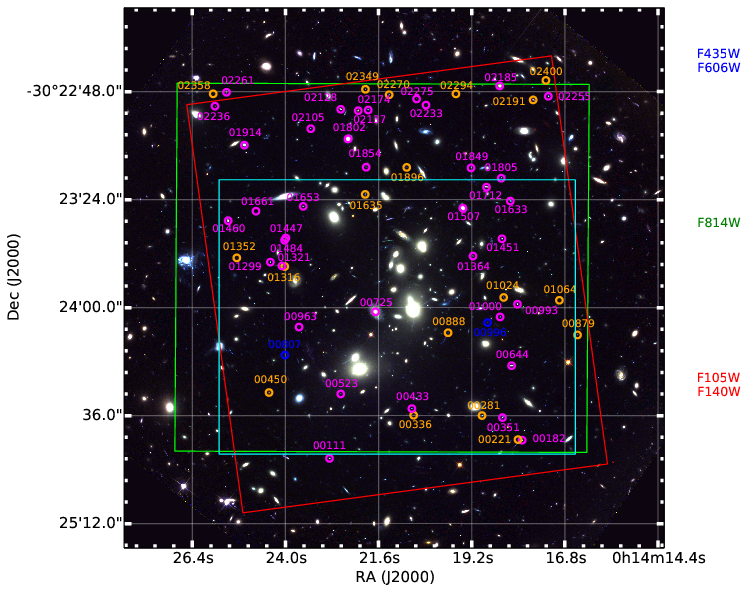
Figure 1.— The color composite image of Abell 2744 based on the HFF and GLASS imaging. The blue, green and red channels are composed by the filters on the right. The two distinct P.A.s of the spectroscopic GLASS pointings are shown by the red (P.A.=233 degrees) and green (P.A.=135 degrees) squares. Figure 2 shows the grism images corresponding to these two P.A.s. The locations of the emission line objects from Table 2 are marked by circles, with color coding reflecting the GLASS spectroscopic redshift quality (cf. Section 4.2 and column “Quality” in Table 2; 2=blue, 3=orange, and 4=magenta). The cyan square shows the outline of Figure 3.

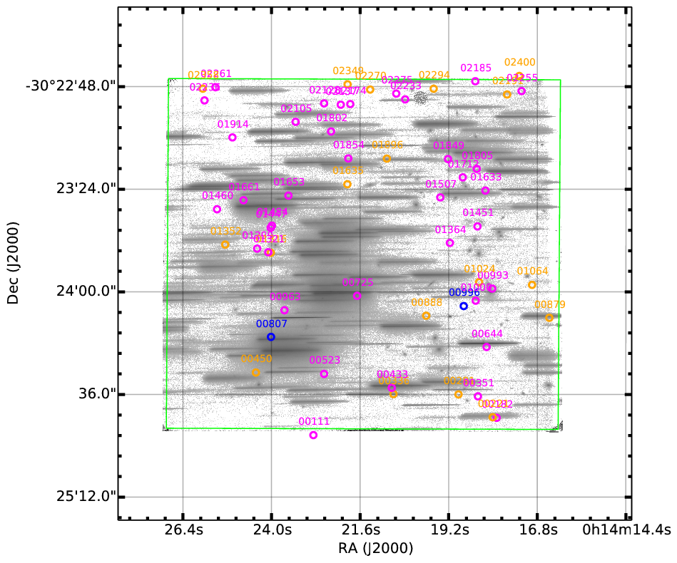
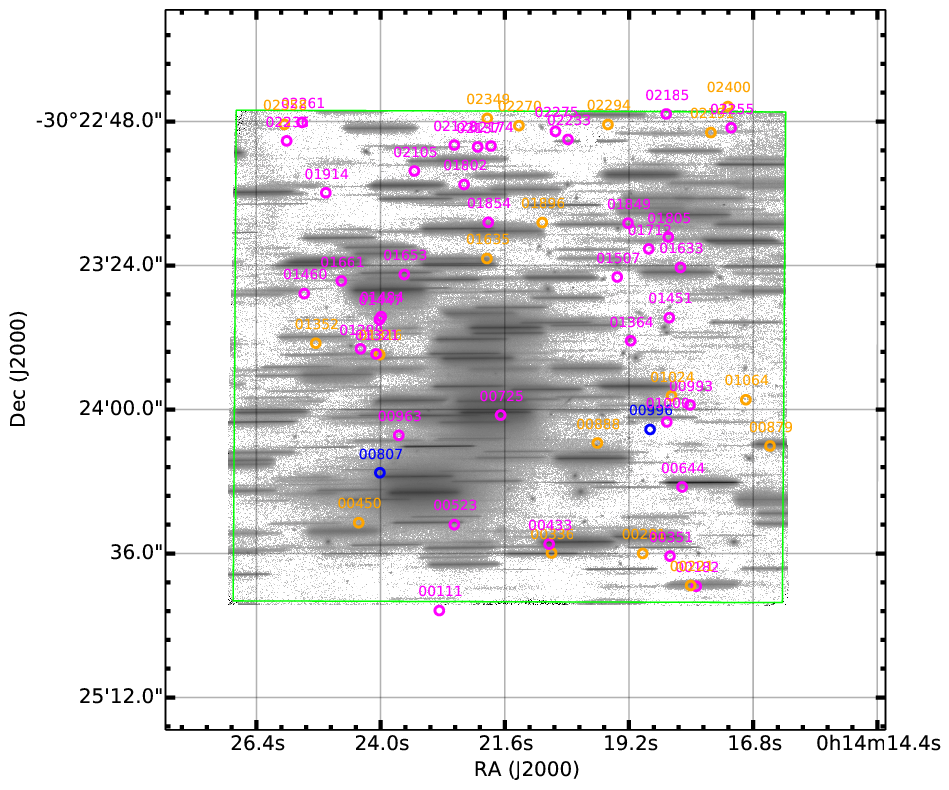
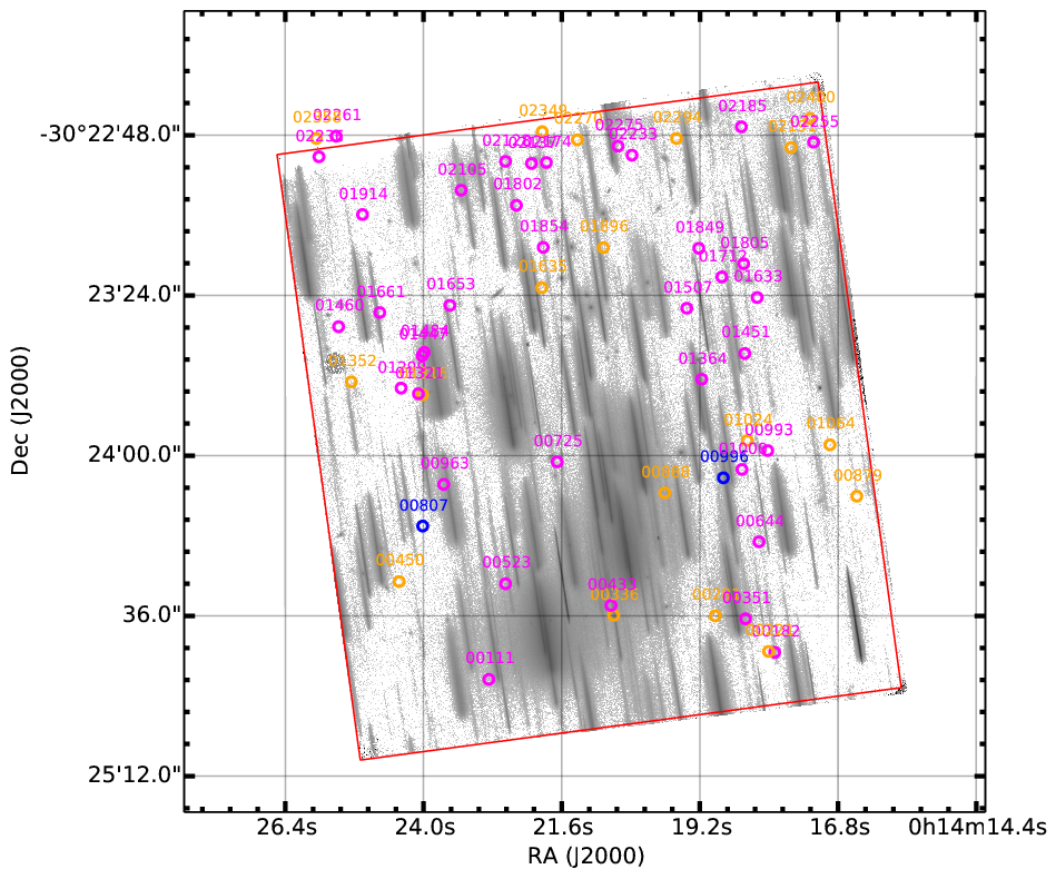
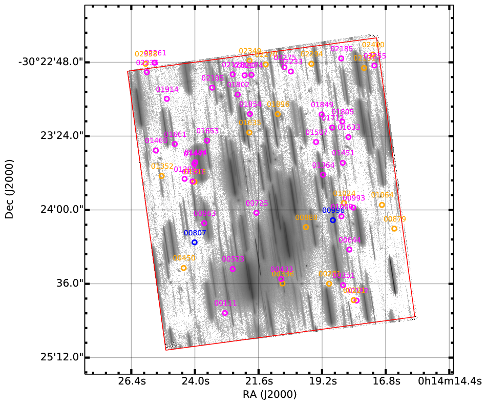
Figure 2.— The GLASS G102 (left) and G141 (right) grism pointings of Abell 2744 at two distinct P.A.s, with field-of-view shown by the red (P.A.=233 degrees) and green (P.A.=135 degrees) squares. The circles in all panels denote the positions of the emission line objects identified in this work, with color coding following the convention adopted in Figure 1.

The GLASS observations are designed to follow the 3D-HST observing strategy (Brammer et al., 2012). The data were processed with an updated version of the 3D-HST reduction pipeline. Below we summarize the main steps in the reduction process of the GLASS data but refer to Brammer et al. (2012) and the GLASS survey paper (Treu et al., 2015) for further details.

The data were taken in a 4-point dither pattern identical to the one shown in Figure 3 of Brammer et al. (2012) to optimize rejection of bad pixels and cosmic rays and improve sampling of the WFC3 point spread function. At each dither position, a combination, a direct (F105W or F140W), and a grism (G102 or G141) exposure were taken. The direct imaging is commonly taken in the filter “matching” the grism, i.e. pairs of F105W-G102 and F140W-G141. However, to accommodate searches for supernovae and the characterization of their curves in GLASS clusters, each individual visit is designed to have imaging in both filters. Hence several pairs of F140W-G102 observations exist in the GLASS data. This does not affect the reduction and extraction of the individual GLASS spectra.

The individual exposures were turned into mosaics using AstroDrizzle from the DrizzlePac (Gonzaga & et al., 2012), the replacement for MultiDrizzle (Koekemoer et al., 2003) used in earlier versions of the 3D-HST reduction pipeline. Then all exposures and visits were aligned using tweakreg, with backgrounds subtracted from the direct images by fitting a second order polynomial to each of the source-subtracted exposures. We subtracted the backgrounds using the master sky presented by Kümmel et al. (2011) for the G102 grism, while for the G141 data the master backgrounds were developed by Brammer et al. (2012) for 3D-HST. The individual sky-subtracted exposures were combined using a pixel scale of $0\farcs 06$ per pixel as described by Brammer et al. (2013) ($\sim$half a native WFC3 pixel) which corresponds to roughly 12Å/pixel and 22Å/pixel for the G102 and G141 grism dispersions, respectively. Figure 2 shows these full field-of-view mosaics of the two NIR grisms (G102 on the left and G141 on the right) at the two GLASS P.A. for Abell 2744. The individual spectra were extracted from these mosaics by predicting the position and extent of each two-dimensional spectrum according to the SExtractor (Bertin & Arnouts, 1996) segmentation maps from the corresponding direct images. This is done for every single object and contaminations, i.e., dispersed light from neighboring objects in the direct image, so these contaminations can be estimated and accounted for.

4. Identification of multiple images

In this section we describe how we identify and vet multiple image candidates using imaging (4.1) and spectroscopic (4.2 and 4.3) data.

4.1. Imaging data: identification and photometric redshifts

Merten et al. (2011) published the first detailed strong lensing analysis of Abell 2744 identifying a total of 34 multiple images (11 source galaxies) in imaging data pre-dating the HFF. With the addition of the much deeper HFF data, now a total of 176/56 candidate arc images/systems have been identified prior to this work (Atek et al., 2014, 2015; Zitrin et al., 2014; Richard et al., 2014; Jauzac et al., 2014; Lam et al., 2014; Ishigaki et al., 2015, see also Figure 3 and Table 1). We identify a new multiply imaged system (i.e. system 60 in Table 1) comprised of three images.

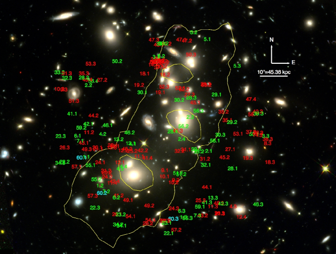
Figure 3.— All multiple images discovered to date in Abell 2744. Green images are used in the lens model, while red images are unused for reasons discussed in Section 4. Cyan images belong to a new multiple image system discovered in this work. The yellow line is the critical curve from our best-fit lens model at $z=9$. The RGB image is a combination of F105W, F125W and F160W.

Despite the vast number of identifications, only a handful of multiple images have been spectroscopically confirmed; arcs 4.3 and 6.1 were spectroscopically confirmed by Richard et al. (2014), arcs 3.1, 3.2 and 4.5 by Johnson et al. (2014), and arc 18.3 by Clément et al. (in preparation). All corresponding redshifts can be found in Table 1. When spectroscopy is lacking, confirming that images belong to the same source is much more difficult. Photometric redshifts alone are not adequate for confirmation. Ilbert et al. (2006) found that, within a given survey, the fraction of catastrophic errors in photometric redshift increases with faintness and redshift. Multiple images are typically faint and are necessarily at redshifts larger than the cluster redshift, which is $z=0.308$ for Abell 2744. The mean F140W magnitude of all images in Table 1 is 27.11, and the mean source redshift is $z=2.63$. Photometry of sources in cluster fields is complicated due to blending with cluster members and the ICL. While we do compute photometric redshifts in order to use the multiple images in our lens model, we do not rely on them alone to test the fidelity of the images.

We instead rely on color and morphology information to determine whether images belong to the same multiple image system; to first order, multiple images of the same source have identical colors. To compute colors, photometry is done using SExtractor in dual-image mode. We use F160W as the detection image because it detects the largest fraction of all multiple image candidates. We then measure isophotal magnitudes and errors in all seven photometric filters. Due to difficulties in detecting many of the multiple image candidates using the default SExtractor settings, we adopt a more aggressive set of settings for the objects with low $S/N$ and/or highly blended. We refer to the default SExtractor settings as “cold” mode and the more aggressive one as “hot” mode photometry. These are similar in spirit but not identical to those adopted by Guo et al. (2013). Even with the “hot” mode settings, we cannot detect all of the multiple image candidates, though the detected fraction is vastly increased over the “cold” mode settings. Using the seven HFF photometric filters, we compute 4 colors for each image: $F435W-F606W$, $F814W-F105W$, $F125W-F140W$, and $F140W-F160W$. The colors are computed within a fixed aperture (MAG_APER) that is $0.4^{\prime\prime}$ in diameter. We compute a reduced “color-$\chi^{2}$” for each image:

$$\chi^{2}_{I\nu}={1\over N-1}\sum_{i=1}^{N}\left({C_{i}-\bar{C}_{i}\over\sigma_{i}}\right)^{2},$$ (1)

where $i$ runs over the number of colors, $N$ is the total number of colors we are able to measure, $C_{i}$ is the $i$-th color, $\bar{C_{i}}$ is the inverse variance-weighted mean color of all images in the system, and $\sigma_{i}$ is the uncertainty in the $i$-th color.

Multiple images of the same source also have predictable morphologies. In rare cases, more than one images of the same source possess a number of uniquely identifiable features. For instance, there are two such systems in Abell 2744, i.e., systems 1 and 2. The counterparts to systems 1 and 2 are systems 55 and 56, respectively. We include both counterpart systems in the lens model at the spectroscopic redshifts of systems 1 and 2 that we measure in this work. All multiple images in Table 1 are visually inspected. We assign each image a grade that determines the likelihood that it is part of the system to which it is assigned. We perform this grading exercise in a lens model-independent fashion; we do not make any assumptions about the location of the critical curves relative to the graded images. There are, however, configurations of multiple images that are impossible to achieve through gravitational lensing by galaxy clusters, such as three individual images (not part of an elongated arc) on the same side of, and very distant from the cluster core with no counter-images. Other information such as surface brightness and symmetry can be incorporated independently of an assumed mass distribution, and we rely on this information much more heavily in assigning the morphology grade. The grading scheme based on morphological similarity is as follows:

4

Image is definitely part of the system

3

Image is very likely part of the system

2

Image is potentially part of the system

1

Image is very unlikely part of the system

0

Image is definitely not part of the system

Two inspectors (A.H. and M.B.) independently assign a grade to each image. The inspectors use several RGB images of the full HFF depth that span the full HST spectral coverage to assign the grade for each image. The two grades are then summed to get the reported morphology grade. Examples of multiple images that receive high and low morphology grades are shown in the Appendix.

We use the color and morphology information together to determine whether to include a multiple image in our model. The joint criteria are:

$$(\chi^{2}_{I\nu}<1.5\quad\lor\quad\textrm{M}>5)\quad\land\quad M>0,$$ (2)

where M is the summed morphology grade from each inspector, which ranges from 0-8. In cases where the contamination by foreground objects, clusters members or ICL is severe, we rely only on the morphology criterion, $M>5$. The particular $\chi^{2}_{I\nu}$ threshold value of $1.5$ was chosen because it is in the typical range for a good reduced chi-square test, and most of the images in spectroscopically confirmed systems are below this value. $M>5$ is chosen because in the least confident case that obeys this, $M=6$, the modelers either both think the image is very likely part of the system ($M=3$) or one thinks the image is potentially part of the system ($M=2$), while the other is sure of it ($M=4$).

For a multiple image system to constrain the lens model, we must estimate its redshift. Having photometric redshift measurements for multiple images of the same source can provide a tighter constraint than a single measurement. Individual photometric redshifts are computed using EAZY (Brammer et al., 2008). We then use a hierarchical Bayesian model to obtain a single redshift probability density function for each system (Dahlen et al., 2013). The mode of this probability density function will be referred to as $z_{\textrm{Bayes}}$. Only non-contaminated objects contribute to calculating $z_{\textrm{Bayes}}$. We graphically outline the procedure for measuring and including photometric redshifts as inputs to our lens model in Figure 4. 2/57 systems (36 and 52) are entirely contaminated, so we do not compute $z_{\textrm{Bayes}}$ for those systems. 14/57 systems have $z_{\textrm{Bayes}}<z_{\textrm{Cluster}}$, and thereby are not included in lens modeling (a fraction of those have poorly constrained posteriors, monotonically declining from 0; they are highly uncertain and considered unreliable; we label them by assigning $z_{\rm Bayes}=0.01$). 5/57 systems have a multi-modal or extremely broad Bayesian redshift distribution. We similarly do not include these systems in the lens modeling. For systems where only one image passed the color/morphology criteria and that image is not contaminated, we report $z_{\textrm{Bayes}}$ in Table 1, but we do not include these systems in the modeling. We show the posterior redshift distributions for some of these cases in the Appendix. System 18 consists of a spectroscopically confirmed image (18.3), but the system as a whole does not pass all criteria required to be considered a multiple image system. Our screening rules out all the above-mentioned systems and delivers a secure set of 25/57 multiple arc systems that are used in lens modeling.

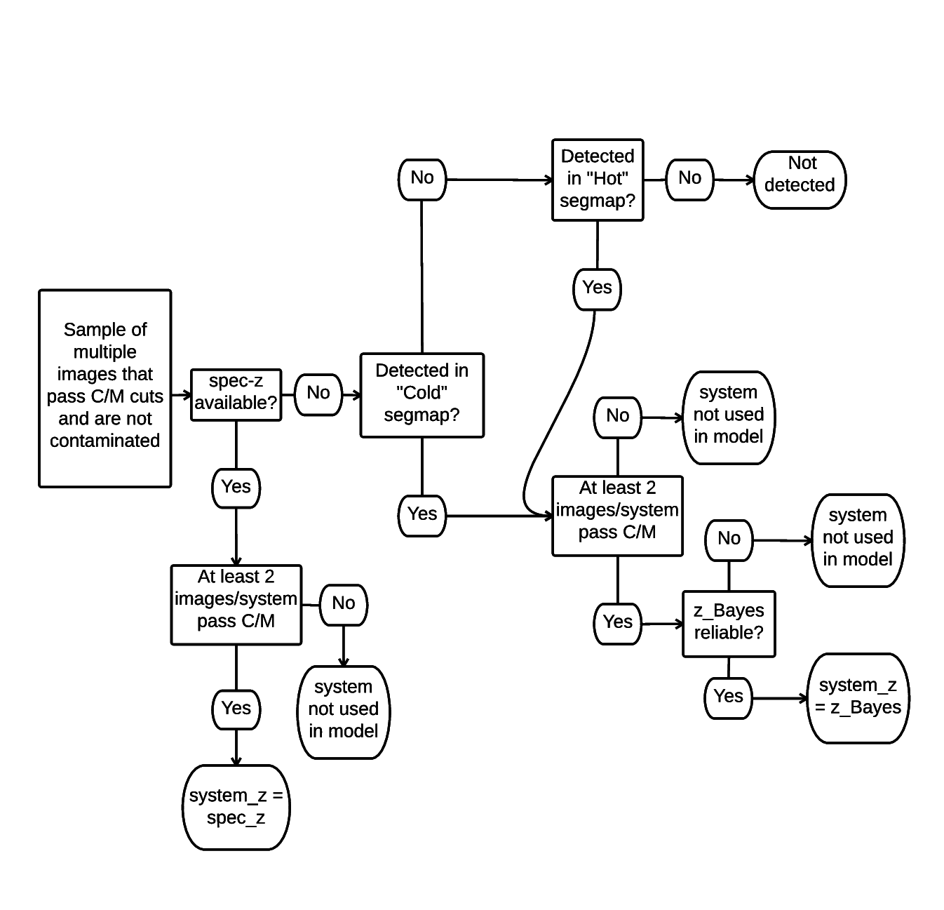
Figure 4.— Flow chart describing our procedure for assigning photometric redshifts to multiple image systems. Two segmentation maps, a “hot” and a “cold” version, were used for source detection. The detection and deblending thresholds are set to the SExtractor defaults in the cold segmentation map. Objects detected in the cold segmentation map, typically the brighter and more isolated ones, have more accurate photometry. The hot segmentation map was created using extremely aggressive detection and deblending thresholds. It detects the majority of the remaining multiple images that are not detected in the cold version. $\textrm{C}/\textrm{M}$ cuts refer to the color/morphology cuts used to purify the sample of multiple images. $z_{\mathrm{Bayes}}$ refers to the redshift obtained from combining multiple redshifts in a hierarchical Bayesian model (Dahlen et al., 2013). $z_{\mathrm{Bayes}}$ is considered reliable if it is larger than the redshift of Abell 2744, $z=0.308$, and it is not multi-valued. See the Appendix for examples of multiple image systems that pass and fail some of the tests in this flow chart.

4.2. Targeted GLASS spectroscopy

GLASS spectroscopy was carefully examined for a total of 179 multiply lensed arc candidates mostly seen on both P.A.s with the goal of measuring spectroscopic redshifts. As described in GLASS paper I, each spectrum was visually inspected by multiple investigators (X.W. and K.B.S.) using the GLASS Graphic User Interfaces (GUIs) GLASS Inspection GUI (GiG) and GLASS Inspection GUI for redshifts (GiGz) The results were then combined and a preliminary list of arcs with emission lines was drafted. In the end, another round of double-check by re-running GiGz was also executed to make sure no potential emission lines were missed. Following GLASS procedure, a quality flag was given to the redshift measurement: Q=4 is secure; Q=3 is probable; Q=2 is possible; Q=1 is likely an artifact. As described in paper I, these quality criteria take into account the signal to noise ratio of the detection, the probability that the line is a contaminant, and the identification of the feature with a specific emission line. For example, Q=4 is given for spectra where multiple emission have been robustly detected; Q=3 is given for spectra where either a single strong emission line is robustly detected and the redshift identification is supported by the photometric redshift, or when more than one feature is marginally detected; Q=2 is given for a single line detection of marginal quality. As shown in Table 2, new spectroscopic redshifts were obtained for 7 images in total, corresponding to 5 systems. Among them, 5 high-confidence (with quality flags 3 or 4) spectroscopic redshifts were measured for arcs 1.3, 6.1, 6.2, 6.3, 56.1. The spectra of these objects are shown in Figures 5–9. In particular for arc 6.1, our spectroscopic redshift matches that reported by Richard et al. (2014), and we provide the first spectroscopic confirmation that 6.2 and 6.3 are images of the same system. We note that our measured redshift for arc 56.1 $z_{\textrm{spec}}=1.20$ (Q=3; probable) differs signficantly from that given by Johnson et al. (2014) for arc 2.1 $z_{\textrm{spec}}=2.2$ (possible), even though the two systems are likely to be physically connected. Our measurement is based on three pieces of evidence. First, we detect a spectral feature in G141 at both P.A.s (see Figure 9 for details) with sufficiently high signal to noise ratio to study its spectra shape. The feature is better described by a single line (identified by us as H$\alpha$ at $z=1.2$) rather than a doublet like [OIII] ($\Delta\chi^{2}=2.4$). Second, a line is marginally detected in one of the G102 spectra at exactly the wavelength expected for [OIII] $z=1.2$. Third, the wide spectral coverage of our data and the data available in the literature rule out the possibility of the feature we see in G141 being other prominent lines such as MgII and [OII]. Taking into account both the evidence and previous results, we assign a quality flag of Q=3 (probable).

The uncertainty on our spectroscopic redshift measurements is limited by the resolution of approximately 50Å and by uncertainties in the zero point of the wavelength calibration. By comparing multiple observations of the same object we estimate the uncertainty of our measurements to be in the order of $\Delta z\sim 0.01$. This is sufficient for our purposes and we will not pursue more aggressive approaches to improve the overall redshift precision (e.g. Brammer et al., 2012).

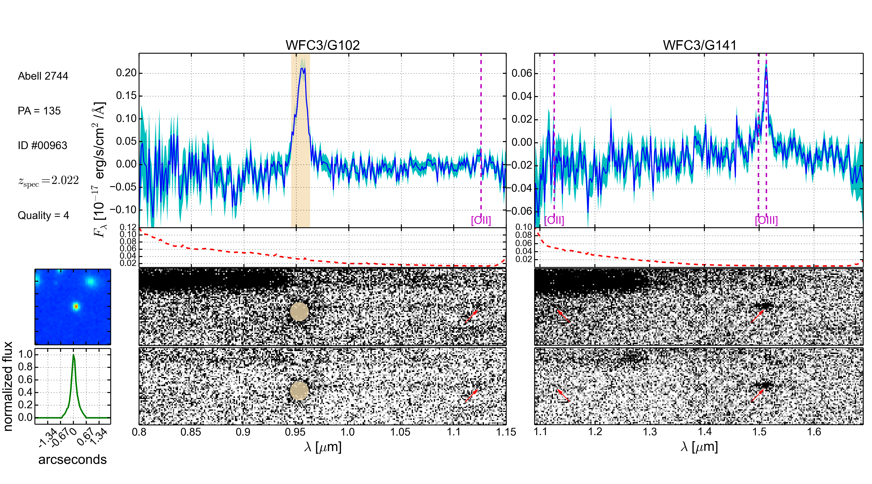
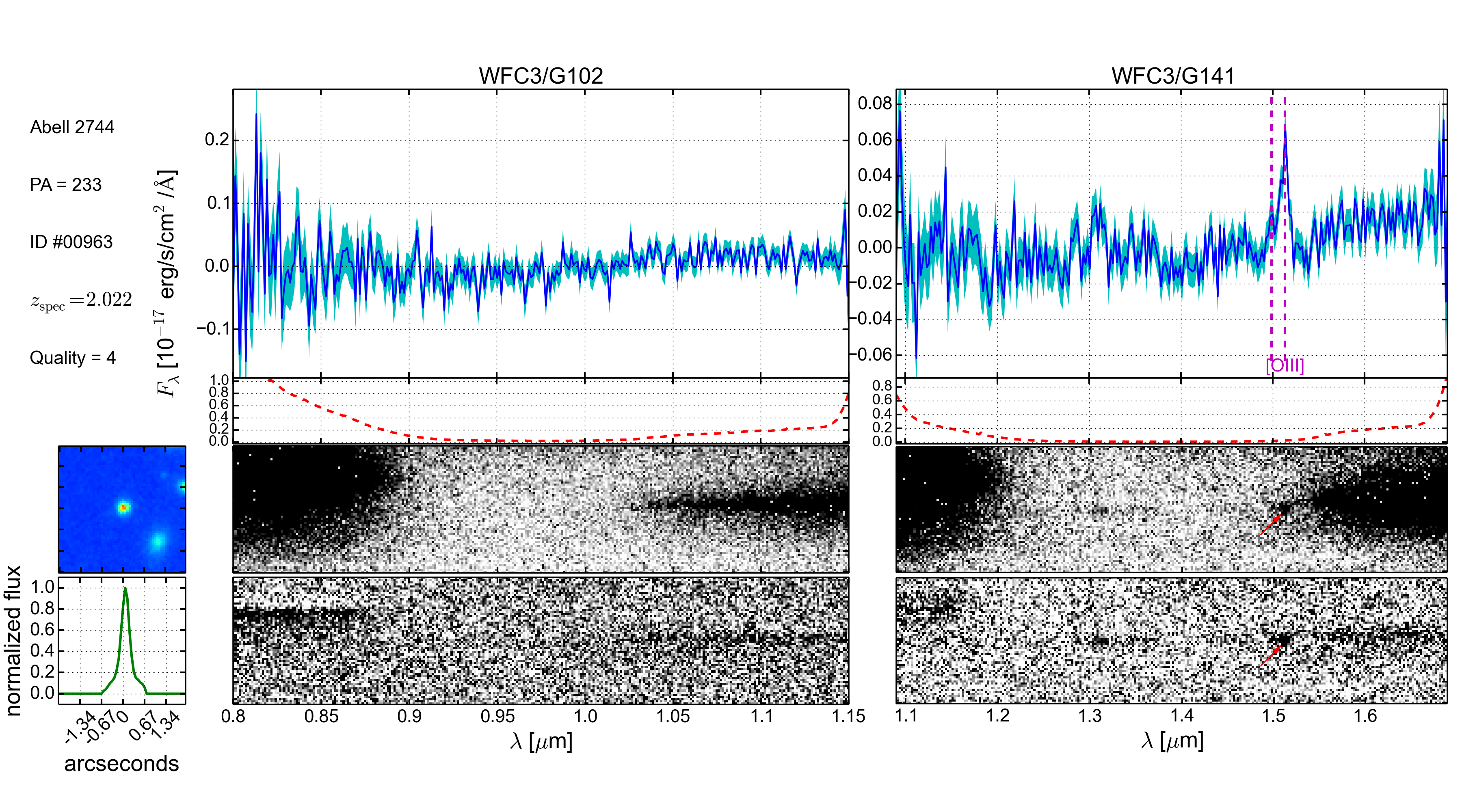
Figure 5.— Emission line detection results on object ID #00963 (arc 6.1) at the two P.A.s displayed in the two sub-figures accordingly. In each sub-figure, the two panels on the first row show the observed 1-dimensional spectra, where the contamination subtracted flux is denoted by the blue solid line and the noise level by the cyan shaded region. The two panels on the second row give the corresponding contamination model in red dashed line. For the four panels directly underneath, the top two display the interlaced 2-dimensional spectra whereas the bottom two have contamination subtracted. In the 1- and 2-dimensional spectra, the identified emission lines are denoted by vertical dashed lines in magenta and arrows in red, respectively. The wheat colored regions cover contamination model defects. The two panels on the far left refer to the 2-dimensional postage stamp created from the HFF co-adds through drizzling (on top) and the 1-dimensional collapsed image (on bottom). Note that these two panels share the same x-axis along the grism dispersion direction. Some ancillary information can also be seen in the upper left corner in each sub-figure.

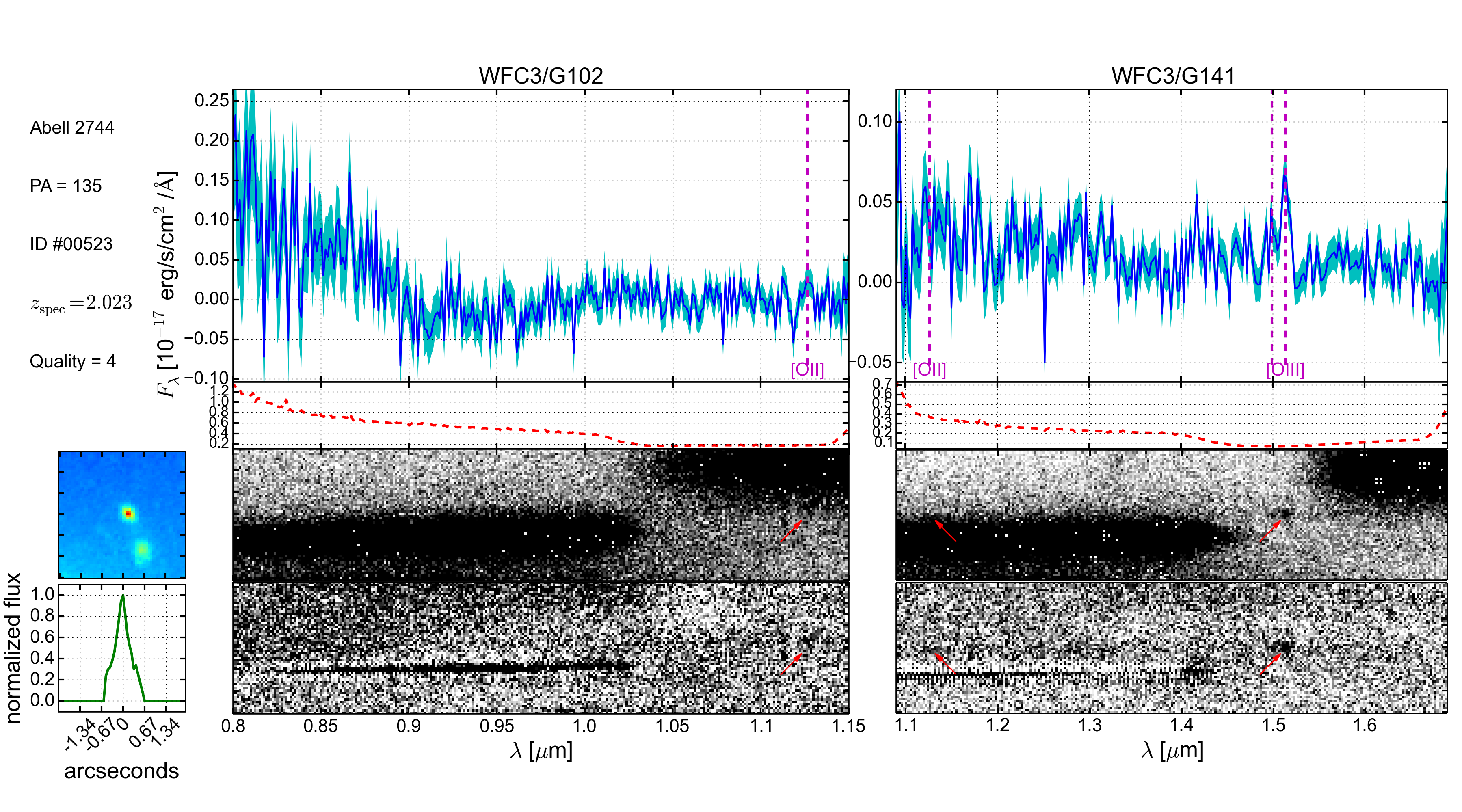
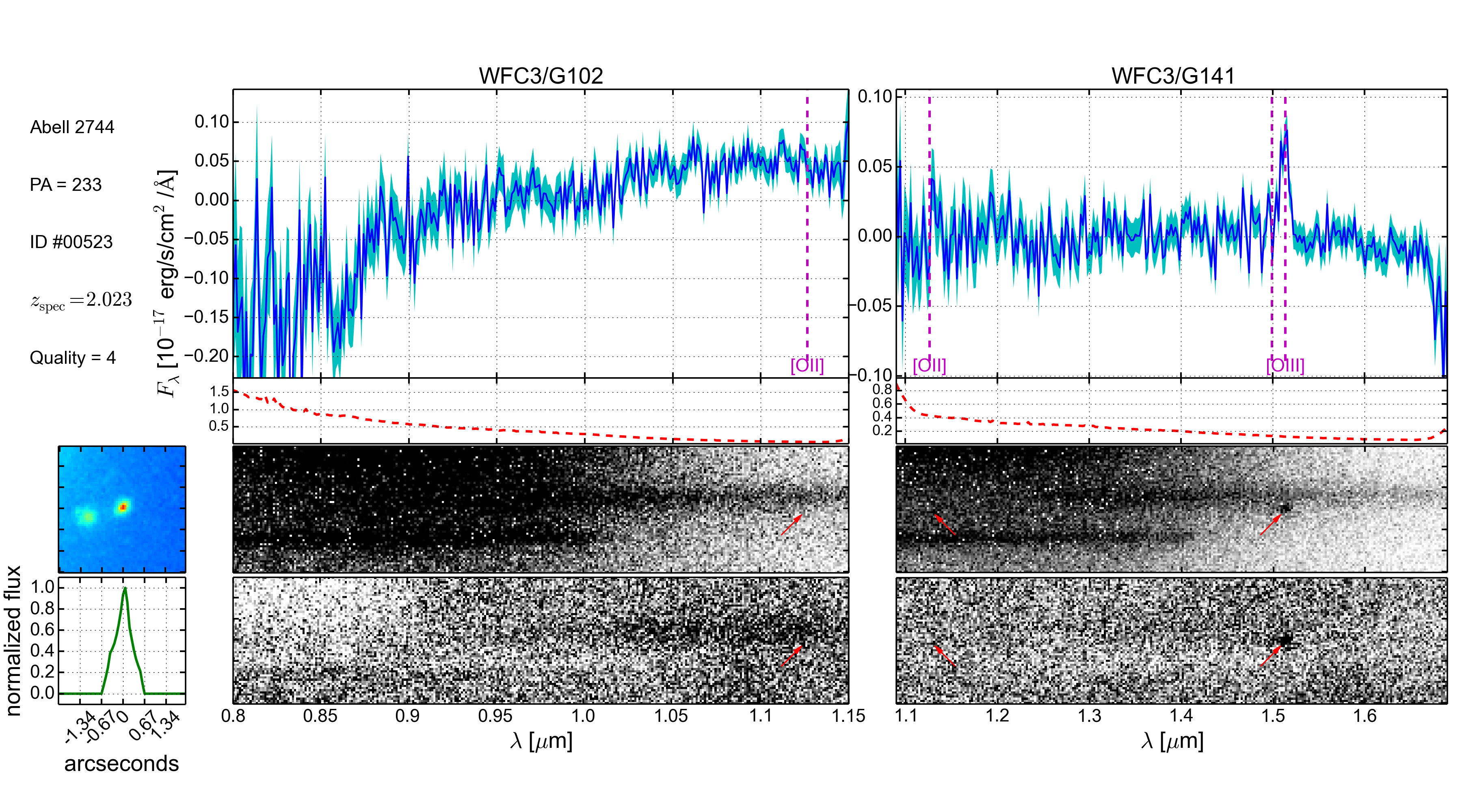
Figure 6.— Same as Figure 5, except that object ID #00523 (arc 6.2) is shown.

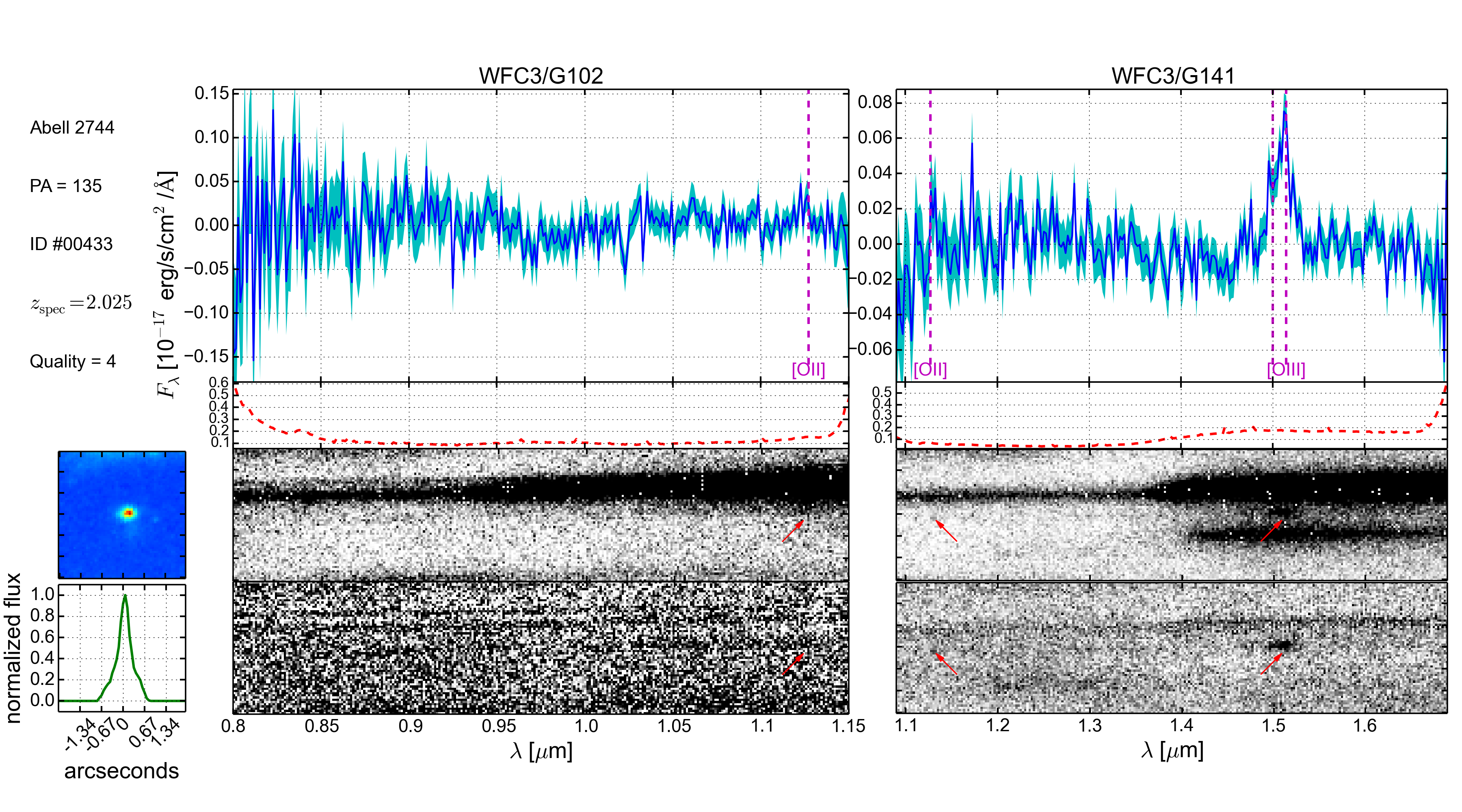
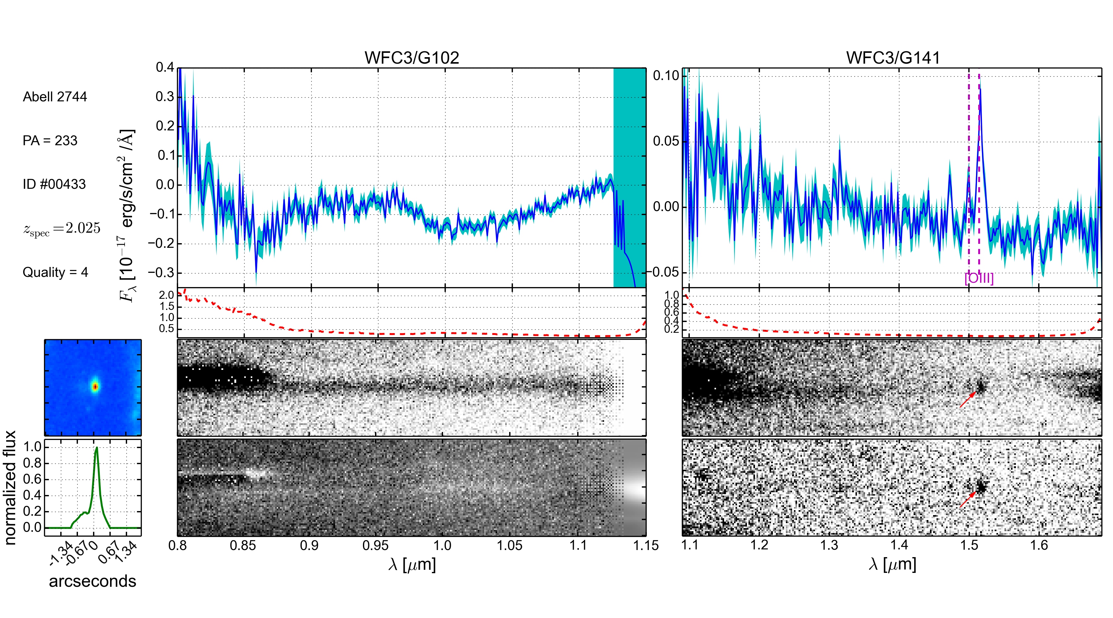
Figure 7.— Same as Figure 5, except that object ID #00433 (arc 6.3) is shown. Note here WFC3/G102 at the second P.A. is cut off on the right due to grism defect.

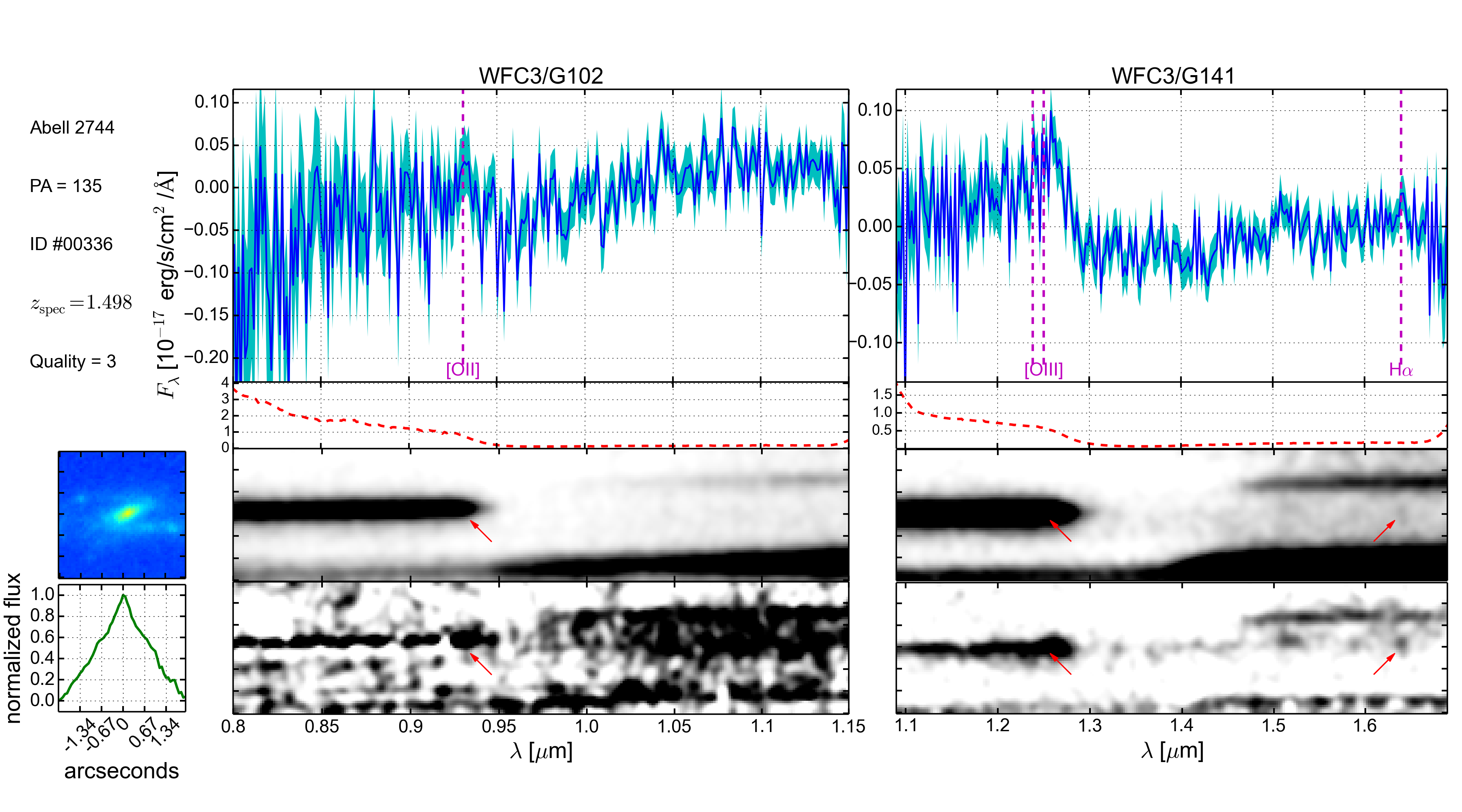
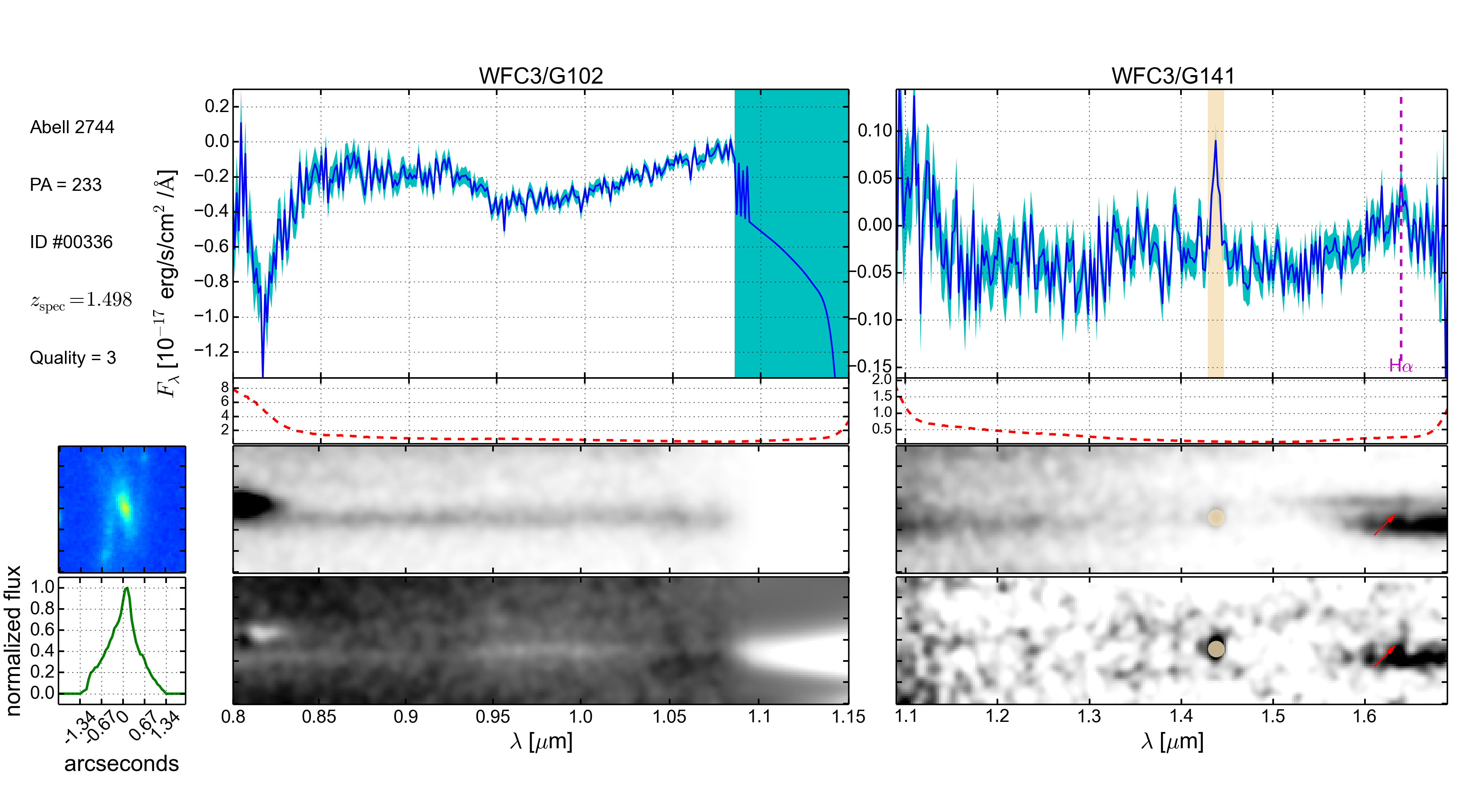
Figure 8.— Same as Figure 5, except that object ID #00336 (arc 1.3) is shown. Moreover, the 2-dimensional spectra are smoothed, whilst the 1-dimensional spectral resolution remains unchanged.

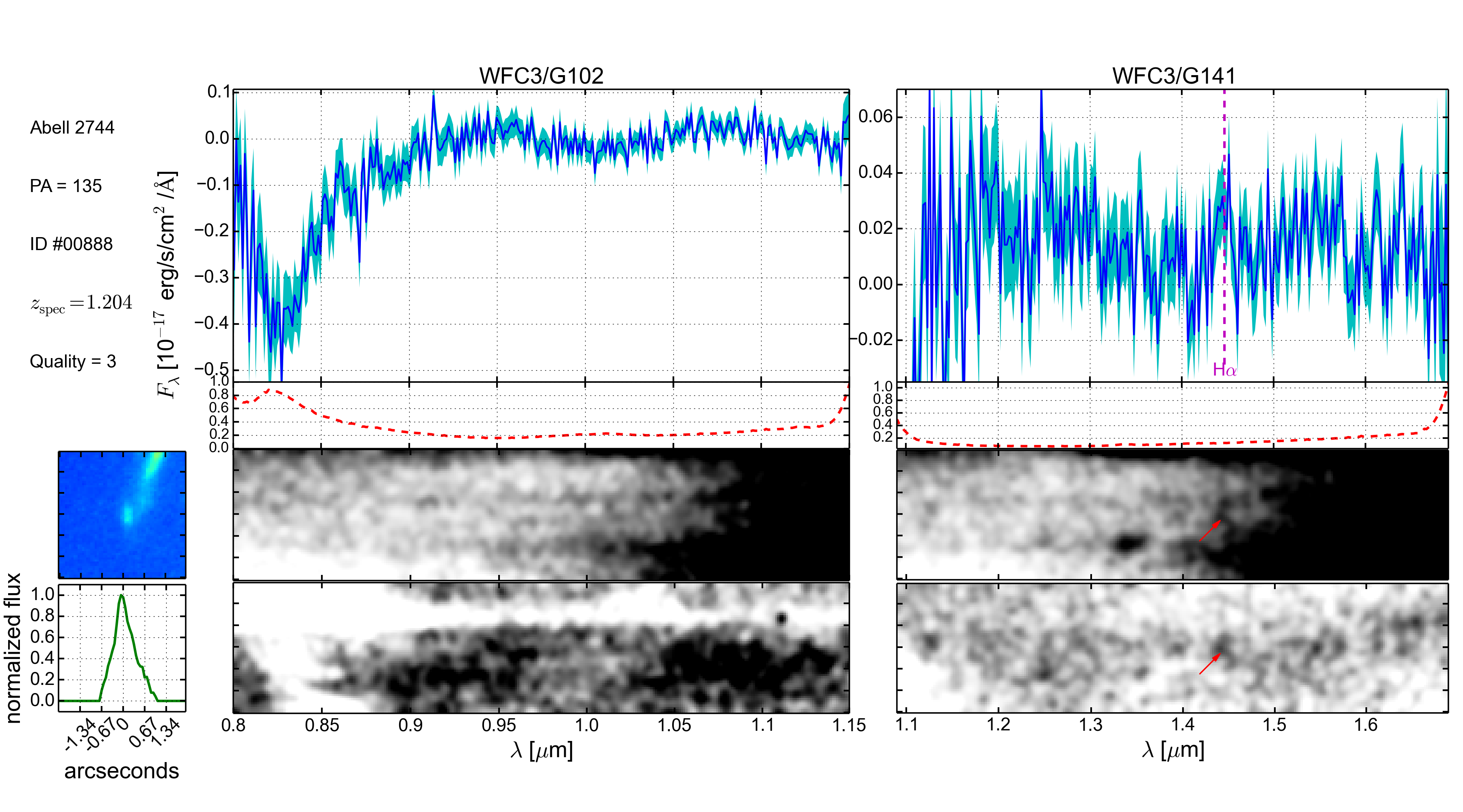
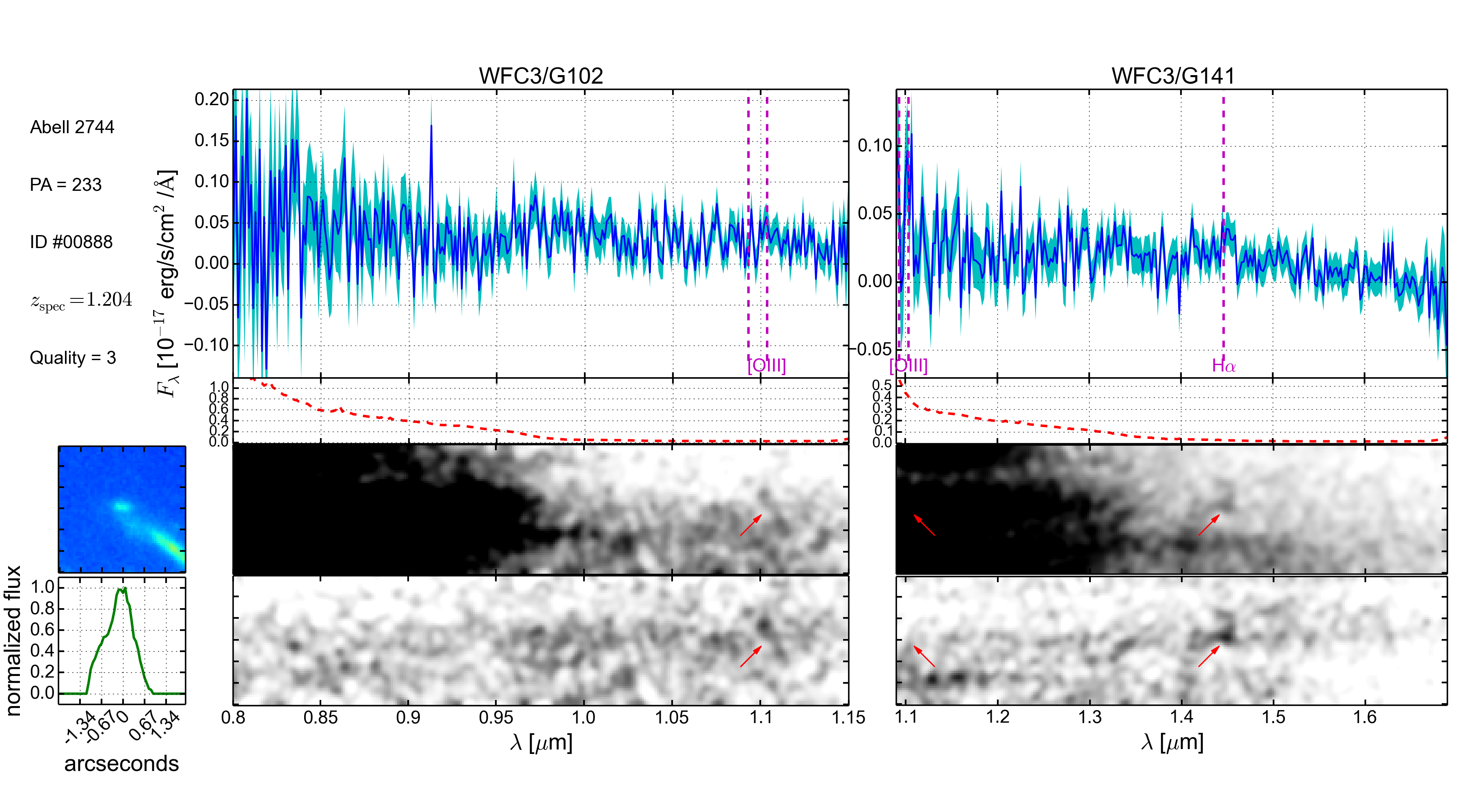
Figure 9.— Same as Figure 8, except that object ID #00888 (arc 56.1) is shown.

4.3. Blind search in GLASS data

The targeted spectroscopy done in Section 4.2 could potentially miss some multiply imaged sources that are not identified photometrically. In order to increase the redshift completeness of emission line sources (both multiply and singly imaged), we also conducted a blind search within the entire grism field-of-view. As a first step, one of us (T.T.) visually inspected all the 2D grism spectroscopic data, the contamination models, and residuals after contamination for each of the 2445 objects in the prime filed of Abell 2744 given by the GLASS catalog. This yielded a list of 133 candidate emission line systems that were later on inspected using the GLASS GUIs GIG and GIGz by two of us (X.W. and K.B.S.) to confirm emission line identifications and measure redshifts. In order to search for previously undiscovered multiple images we inspected each set of objects with mutually consistent redshift. None of the sets of galaxies at the same spectroscopic redshifts are consistent with being multiply lensed images of the same source. Some of them are ruled out because of their position in the sky, while others are ruled out because their colors and morphology are inconsistent with the lensing hypothesis.

Nonetheless, we compiled a list of singly imaged emission line objects, consisting of 18, 16, and 34 quality 2, 3, and 4 spectroscopic redshift measurements respectively, which are color coded in Figure 1. Among them, the high-confidence (with quality flag 3 or 4; orange and magenta circles in Figure 1) emission line identifications are also included in Table 2. As mentioned in Section 4.1, via running EAZY on the full-depth seven-filter HFF imaging data, we were able to measure photometric redshifts for those objects as well. As a result, a comparison between spectroscopic and photometric redshift measurements is possible, as displayed by Figure 10. We find that 25/55 photometric redshifts agree within their 1-$\sigma$ uncertainties with corresponding spectroscopic redshifts, when nebular emission lines are included in the fitting template. This suggests the presence of additional systematic errors that are likely related to the photometric redshift fitting method. In order to account for the unknown systematics, we increase the photometric redshift uncertainties for the sources used in the construction of the lens model.

We double-checked our spectroscopic redshift measurements by re-running GiGz on all the objects and also cross-checked the photometric redshift measurements through re-fitting the photometric redshifts using a different method by a subset of the authors (R.A., M.C., E.M) without knowing previous results. The general conclusions about the agreement between spectroscopic and photometric analyses remains unchanged.

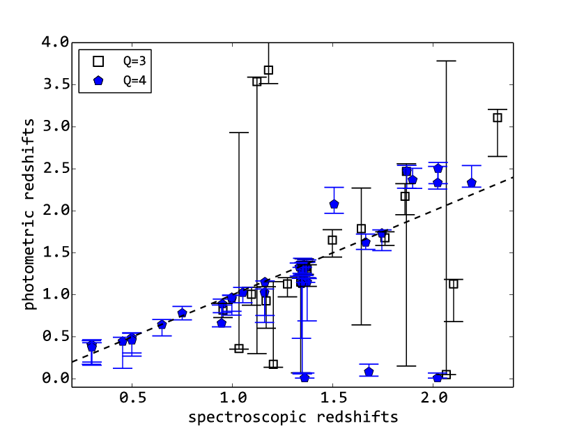
Figure 10.— Comparison between the spectroscopic and photometric redshifts for the 55 objects with high-confidence emission lines (quality flags 3 or 4). We also show the 1-$\sigma$ error bars (enclosing 68% of the total probability) around the photometric redshifts. There is reasonably good agreement between photometric and spectroscopic redshifts, with 25 out of 55 spectroscopic redshifts within the photometric redshift error bars. This is acceptable considering that the photometric redshift uncertainties only include the random component, even though they suggest that an additional systematic uncertainty component is present. In order to account for this systematic uncertainty, for the systems used to build the lens model we added 20% in quadrature to our photometric errors.

5. Gravitational Lens Model

Our lens modeling method, SWUnited (Bradač et al., 2009, Bradač et al., 2005), constrains the gravitational potential within a galaxy cluster field via $\chi^{2}$ minimization. It takes as input a simple initial model for the potential. A $\chi^{2}$ is then calculated from strong and weak gravitational lensing data on an adaptive, pixelated grid over the potential established by the initial model. The number of grid points is increased and the $\chi^{2}$ is recalculated. Once the minimum is found, and convergence is achieved, derivative lensing quantity maps, such as convergence ($\kappa$), shear ($\gamma$) and magnification ($\mu$), are produced from the best-fit potential map. Errors in these quantities are obtained via the method described below. Maps of the convergence and magnification are shown in Figure 11.

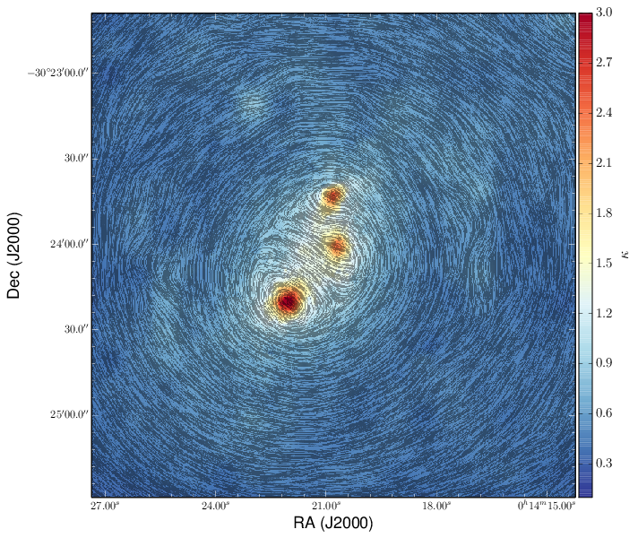
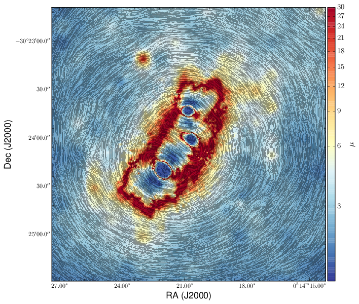
Figure 11.— Convergence (left), $\kappa$ and flux magnification (right), $\mu$, maps of Abell 2744 produced by our lens model for a source at $z=9$. Maps cover $3.5\times 3.5\,\textrm{arcmin}^{2}$. In both maps, the gray stick pattern indicates the phase angle of the shear. The figures are made using software written by Dan Coe.

A previous model of Abell 2744 using pre-HFF data was created using the same lens modeling code. The model was created as part of a call by STScI to model the HFF clusters, and it appears on the publicly accessible HFF lens modeling website as the Bradac v1 models. The previous model was constrained using 44 total multiple images belonging to 11 distinct systems. The weak lensing constraints were obtained by one of the modelers, Julian Merten, and distributed to all participating modeling teams. The same weak lensing constraints were used in the model that appears in this work. This model is also made available to the public on the HFF lens modeling website as the Bradac v2 model. In the v1 model, magnification uncertainties were estimated by bootstrap-resampling the weak lensing galaxies. In this work, however, we took a different approach to estimate uncertainties, one that we expect more accurately represents the true uncertainties. Because the number of multiple image systems used in this model is much larger than in the v1 model, 72 total multiple images belonging to 25 distinct systems, we bootstrap-resampled the multiple image systems that were not spectroscopically confirmed. These are the systems for which we use $z_{\textrm{Bayes}}$ in the lens model. We assess the impact of photometric redshift uncertainty on the derived lensing quantities by resampling the redshift of each system lacking spectroscopic confirmation from their full $z_{\textrm{Bayes}}$ posteriors. We compare the variance in magnification due to redshift uncertainty with the variance in magnification due to bootstrap-resampling the multiple image systems, finding that the latter is dominant. We nonetheless propagate both sources of error when reporting the errors on all derived lensing quantities in this work.

As a test of the improvement of the lens model with the addition of the new multiple image constraints from the HFF data, we calculate the magnification of SN HFF14Tom, a Type Ia Supernova (SN Ia) at $z=1.35$ discovered in the primary cluster field of Abell 2744 (Rodney et al., 2015). We compare the magnification predicted by our lens model with the magnification calculated directly from a comparison with other SNe Ia at similar redshifts, $\mu=2.03\pm 0.29$ (Rodney et al., 2015). The magnification predicted by the v1 model, using pre-HFF data was $\mu_{\mathrm{best}}=3.15$, with $\mu_{\mathrm{median}}=2.45^{+0.19}_{-0.16}$ ($68\%$ confidence). The new model presented in this work, v2, predicts a consistent magnification of $\mu_{\mathrm{best}}=2.23$, with $\mu_{\mathrm{median}}=2.24^{+0.07}_{-0.08}$ ($68\%$ confidence). The improved lensing constraints significantly improve the accuracy as well as the precision according to this test. We note that while we were not blind to the magnification of the supernova predicted by Rodney et al. (2015) when producing the v2 lens model, we did not use the magnification as an input to our model.

5.1. Comparison with previous work

Three teams (Jauzac et al., 2014, Lam et al., 2014 and Ishigaki et al., 2015) have published models of Abell 2744 using new multiple image constraints identified in the HFF imaging data. Of these teams, currently only the lens models produced by Ishigaki et al., 2015 (GLAFIC) are publicly available through the Mikulski Archive for Space Telescopes (MAST). We compare our models to theirs as well as the Sharon v2 models, which include updated spectroscopic measurements of multiple images identified before the HFF data were obtained (Johnson et al., 2014). Finally, we also compare our model with several updates of the CATS(v1) models (Jauzac et al. 2015, private communication). The CATS(v2) models are presented by Jauzac et al. (2014) and use a much larger number of multiple images than we include in our lens model. CATS(v2.1) employs the same set of multiple images as CATS(v2), but makes use of the spectroscopic redshifts obtained in this work. CATS(v2.2) uses the same set of multiple image constraints used in our model. We compare the surface mass density profiles (Figure 12) and cumulative magnified source plane areas (Figure 13) predicted by all models described above. The surface mass density profiles agree quite well at radii where multiple image constraints are plentiful. However, the models begin to differ rapidly near the boundaries of the constrained area. Our model disagrees with the CATS models most severely. It is interesting to note that the three CATS models agree internally extremely well, despite CATS(v2.2) using the same set of multiple images used in this work, a considerably different set than the one used in CATS(v2) and CATS(v2.1). The significant difference between our model and the CATS models may be due to differences in the modeling techniques or the fact that our method uses additional constraints (weak lensing). Weak lensing constraints have a stronger impact on the model at radii beyond where multiple images are observed. In contrast, there is excellent agreement among the models in the inferred magnified source plane area. Thus, even though there may be small but significant differences in the specific details of each reconstructions, by and large the total integrated properties are very similar.

We also note that our model supersedes the model obtained by members of our team as part of the initial HFF modeling effort based on pre-HFF data. The uncertainties in this current version of the model are smaller, consistent with the fact that we have increased the number of strong lensing constraints.

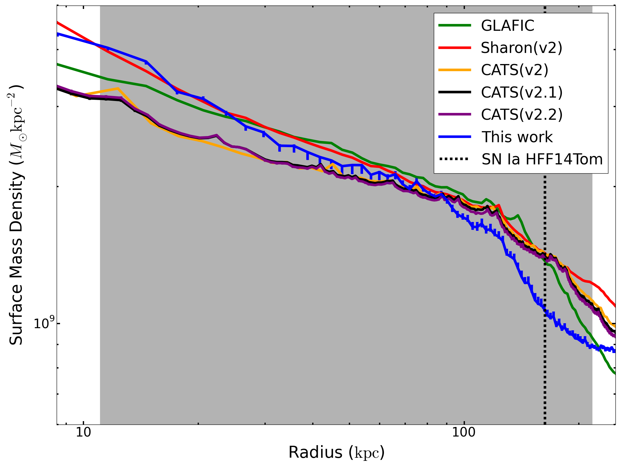
Figure 12.— Surface mass density profile for the lens model obtained in this work compared to several recently published lens models of Abell 2744. The Sharon v2 model is presented by Johnson et al. (2014), the GLAFIC model by Ishigaki et al. (2015), the CATS(v2) model in Jauzac et al. (2014), and the CATS(v2.1) and CATS(v2.2) models by Jauzac et al. (2015, private communication). The shaded gray region indicates the radii over which multiple image constraints are available. The models agree best within this region, and they begin to significantly disagree at radii $\gtrsim 200$kpc. The radius is measured from the center of the BCG. Error bars shown for our model represent $68\%$ confidence. Gaussian 1-$\sigma$ error bars are included on all three CATS models, but are almost entirely too small to discern.

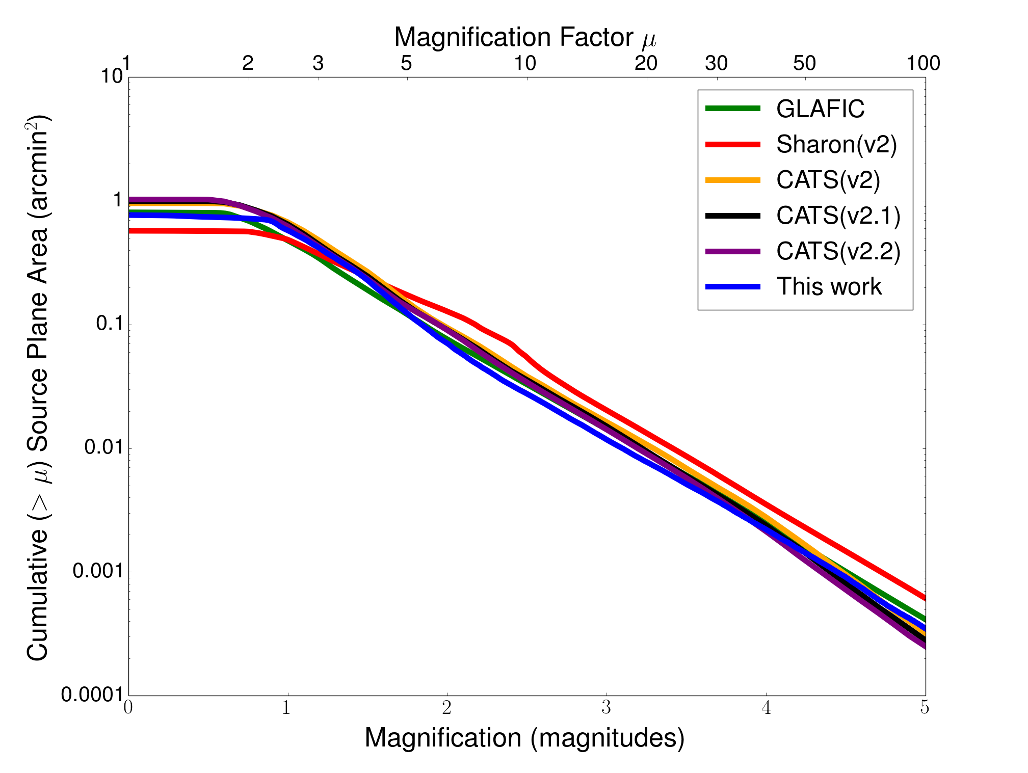
Figure 13.— Cumulative source plane area versus magnification at $z=9$. The models used in this comparison are the same as those described in Figure 12.

We also compare our method of estimating redshifts of multiple image systems with the one used by the CATS team (Richard et al., 2014, Jauzac et al., 2014). In Figure 14, $z_{\textrm{Bayes}}$ is the redshift obtained from hierarchical Bayesian modeling of the photometric redshifts obtained in this work. $z_{\textrm{model}}$ is the redshift obtained by Jauzac et al. (2014) by minimizing their analytical model uncertainty while leaving the redshift as a free parameter. It is important to check this procedure independently since leaving $z_{\textrm{model}}$ as a free parameter or predicting additional multiple images that belong to the same system could in principle lead to confirmation bias. Overall, we find good agreement between $z_{\textrm{Bayes}}$ and $z_{\textrm{model}}$, within the admittedly large uncertainties on $z_{\textrm{Bayes}}$. There are only two new systems with spectroscopic redshifts available to compare with $z_{\textrm{model}}$, and they are both inconsistent at $>5\sigma$. This may be due to small number statistics or perhaps an indication that the uncertainties on $z_{\textrm{model}}$ are underestimated. More spectroscopic redshifts are needed to perform this test in a more stringent manner.

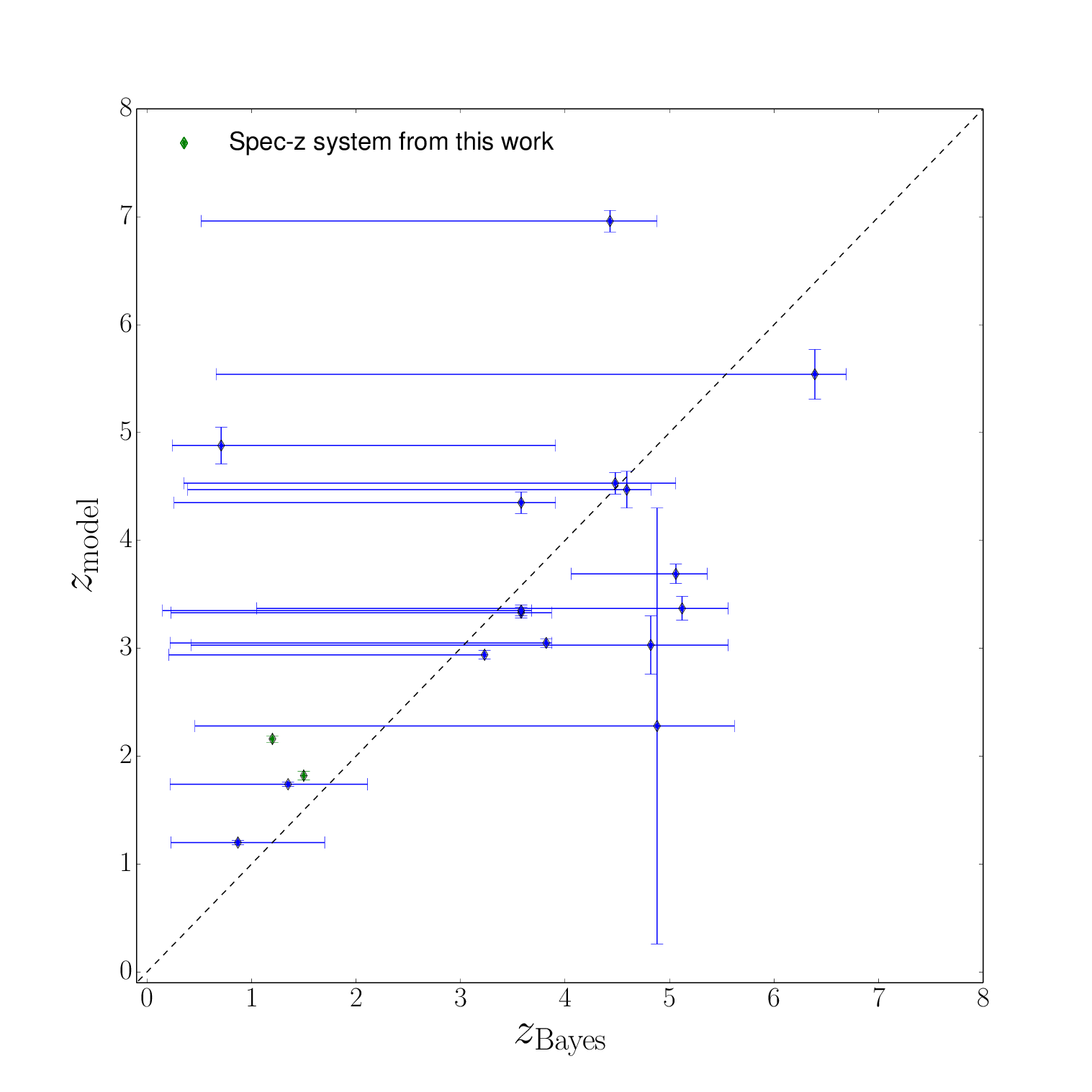
Figure 14.— Comparison of the redshifts determined in this work ($z_{\textrm{Bayes}}$) versus the model-predicted redshifts given by Jauzac et al. (2014) for all multiple image systems used in the lens model. Note that the previously confirmed spectroscopic systems are left out of this comparison because $z_{\textrm{m}odel}$ were not calculated. Two systems (green) are spectroscopically confirmed in this work for the first time and are included in the comparison. For these two objects, we use the new spectroscopic redshift on the horizontal axis in place of $z_{\textrm{Bayes}}$. The $z_{\textrm{model}}$ values are in significant disagreement with the spectroscopic values for these two systems. $z_{\textrm{Bayes}}$ represents the peak of a statistical combination of all available photometric redshift probability density functions (Dahlen et al., 2013). The vertical error bars reflect 1-$\sigma$ Gaussian error on $z_{\textrm{model}}$, and the horizontal error bars show the $68\%$ credible interval for $z_{\textrm{Bayes}}$. 12/16 systems are consistent at $68\%$ confidence level.

6. The spatial distribution of stellar and dark matter

6.1. Stellar mass map

The Spitzer IRAC $3.6\,\mu$m image samples close to rest-frame $K$-band for the cluster, so we use the $3.6\,\mu$m fluxes from cluster members to approximate the cluster stellar mass distribution. We first selected the red sequence cluster members brighter than the 25th mag in F814W from the color-magnitude and color-color diagrams following the procedure described in Richard et al. (2014). We also cross-matched the selected cluster members with the spectroscopic redshift catalog given by Owers et al. (2011) to ensure that we included all the cluster members confirmed with spectroscopy. We selected a total of 190 bright cluster members for their stellar mass distribution.

To create an image with $3.6\,\mu$m flux from cluster members only, we first created a mask with value 1 for pixels that belong to cluster members in the F160W image and 0 otherwise. We then convolved the mask with the $3.6\,\mu$m PSF to match the IRAC angular resolution, set the pixels below 10% of the peak value to zero, and resample the mask onto the IRAC pixel grid. We obtained the $3.6\,\mu$m map of cluster members by setting all IRAC pixels not belonging to cluster members to zero and smoothed the final surface brightness map with a two-pixel wide Gaussian kernel.

The IRAC surface brightness map was transformed into a surface mass density map by transforming the 3.6$\mu$m flux into K-band luminosity and then by multiplying by stellar mass to light ratio derived by Bell & de Jong (2001) using the so-called “diet”-Salpeter stellar initial mass function (IMF). The resulting stellar mass map in show in the left panel of Figure 15.

The main source of uncertainty on the stellar mass density is the unknown initial mass function. For example, if one were to adopt a Salpeter (1955) IMF – as suggested by studies of massive early-type galaxies, the stellar mass density would increase by a factor of 1.55.

6.2. Stellar to total mass ratio

We obtain the stellar to total mass ratio map by dividing the stellar surface mass density map obtained from photometry by the total surface mass density map obtained from gravitational lensing. This is shown in the right panel of Figure 15. We note that resolution effects are non-trivial to take into account, since the resolution of the lensing map depends on the density of local sources and the amount of regularization. Thus, the map should be interpreted keeping in mind this caveat. Interestingly the stellar to total mass ratio varies significantly across the cluster. Many but not all the massive ellipticals seem to reach values of 0.05 or more, which are typical of the central regions of isolated massive galaxies (e.g. Gavazzi et al., 2007). However, the ratio appears to be significantly lower in the center of the cluster and in the south-east quadrant. In future work, we plan to compare the observed map with those obtained from numerical simulations by taking into account the effects of finite resolution in the observed mass and light maps, in order to test whether the spread in stellar to total mass ratio is reproduced. Furthermore, we plan to carry out a systematic comparison with mass reconstructions where mass is assumed to follow light up to a scale factor (Zitrin et al., 2009). At face value our result is inconsistent with this assumption for a merging cluster like Abell 2744. However, uncertainties on both models and resolution effects must be taken into account in order to evaluate the significance of this apparent violation. Thus, this result should be considered as preliminary until confirmed by a more detailed analysis.

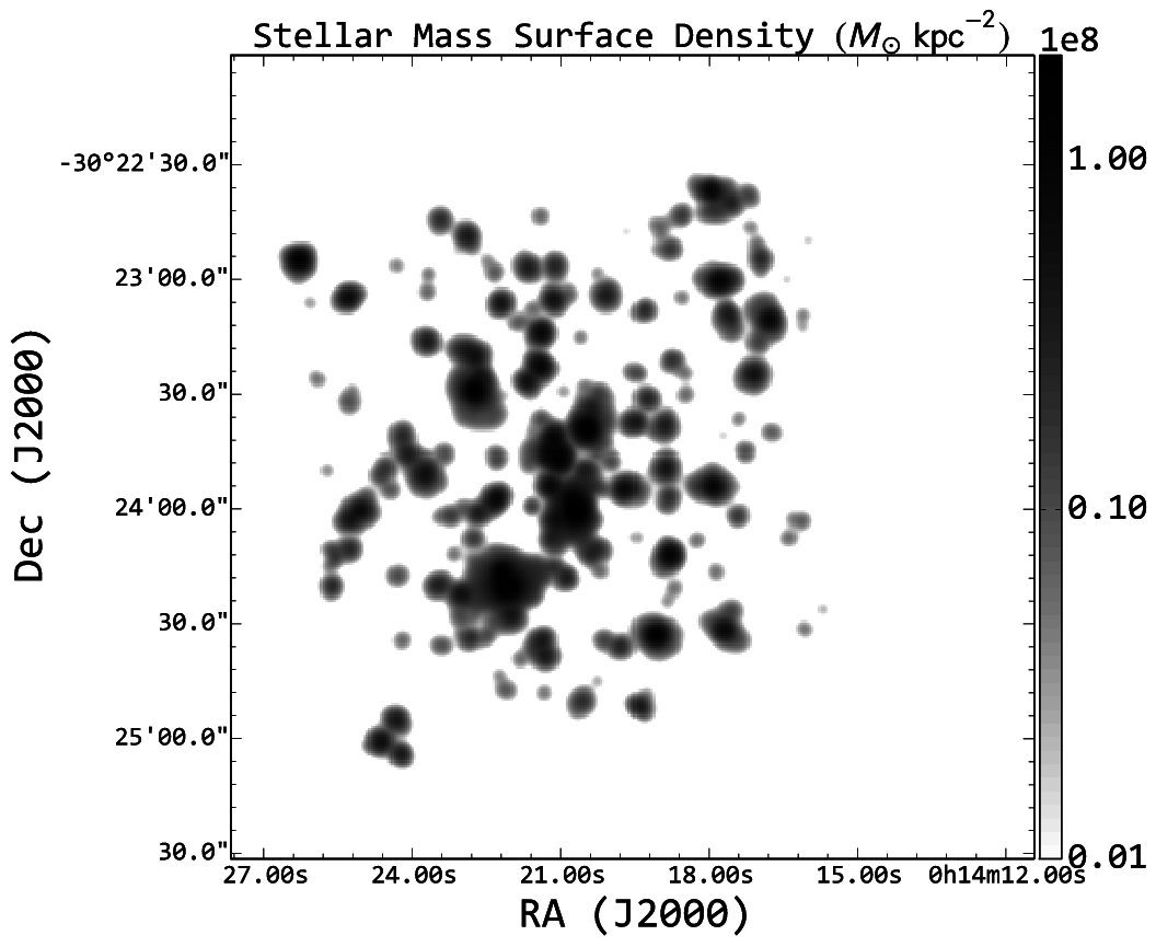
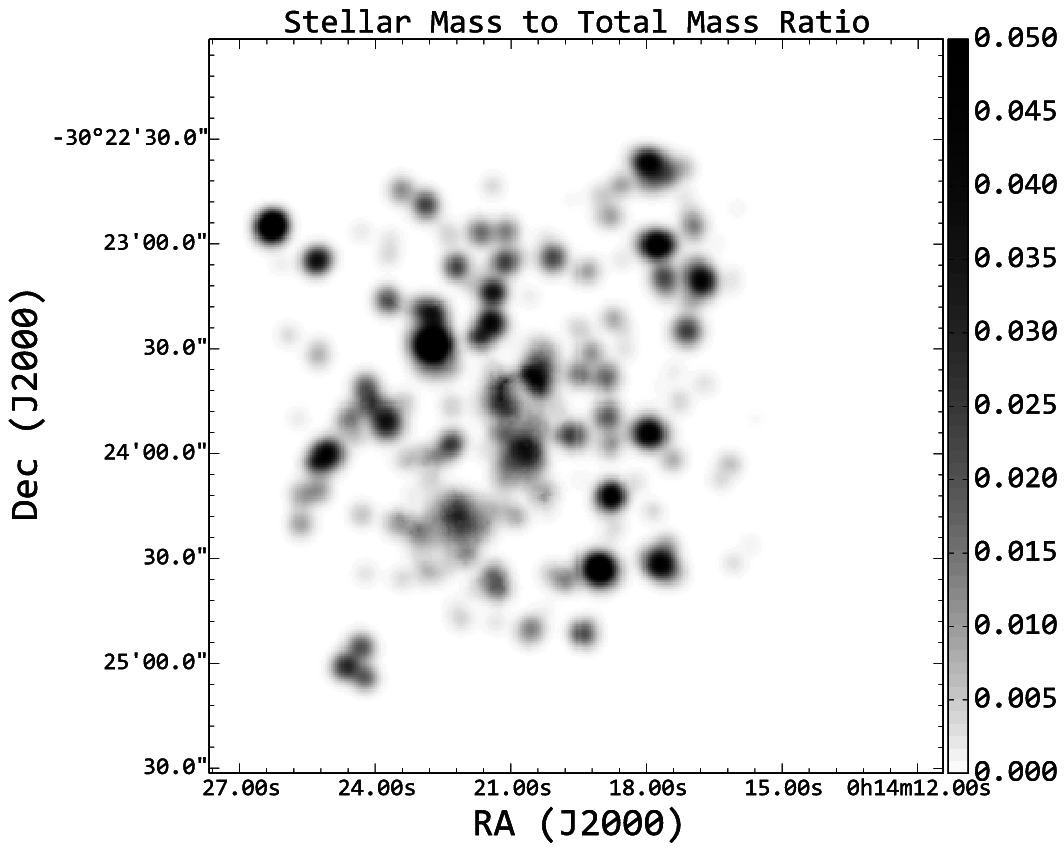
Figure 15.— Stellar mass surface density (left) and stellar to total mass ratio (right) distributions of Abell 2744. Stellar mass surface density is in the unit of $M_{\odot}\,\text{kpc}^{-2}$.

7. Conclusions

In this paper we have used spectroscopic data from the GLASS survey in combination with ultra-deep imaging data from the HFF program to construct a strong gravitational lens model for the cluster Abell 2744. In an effort to obtain a precise and accurate mass model we carried out a systematic search for spectroscopic redshifts of multiple images and we applied a rigorous algorithm to select only secure multiple image systems amongst the dozens that have been proposed in the literature. The lensing mass map is then combined with a stellar mass map derived from IRAC photometry to study the relative spatial distribution of luminous and dark matter. Our main results can be summarized as follows:

1. We have measured spectroscopic redshifts for 5 multiple image systems (quality flag 4 and 3, i.e. secure and probable). We have also confirmed spectroscopically that images 6.1, 6.2, 6.3 belong to the same source. The spectroscopically confirmed images are used to constrain the gravitational lens model. We also obtain 2 tentative redshifts, which are not used to to constrain the mass model, but could potentially be confirmed by future work.

2. From the GLASS data we derive an extensive redshift catalog of faint emission line systems which we use to test photometric and lensing determinations of redshift. Generally speaking, the measurements agree within the 1-$\sigma$ uncertainties, when nebular emission lines are included in the fitting template. In addition, we compare photometric redshifts with redshifts determined by Jauzac et al. (2014), based on their gravitational lens model and find an agreement within the large uncertainties of the former. For the two systems with new spectroscopic redshifts we find a significant difference with respect to model redshifts. This may be due to small number statistics or to the model redshifts uncertainties being underestimated. More spectroscopic redshifts are needed to make a more stringent test.

3. Our rigorous selection algorithm identifies a total of 25/72 multiple arc systems/images as secure out of a sample of 57/179 candidate multiple arc systems/images, compiled from the literature and from our own work. Most systems are rejected either on the basis of inconsistent morphology or inconsistent spectral energy distribution between the candidate multiple images, or because of insufficient evidence that they belong to the same source.

4. The derived mass model is found to be very precise, as measured by bootstrap- and redshift-resampling the set of multiple images used as input. Furthermore, we tested how well our model reproduces the magnification of the background SN Ia Tomas (Rodney et al., 2015). The SN Ia was not used as a constraint to the model and yet its magnification is consistent ($2.03\pm 0.29$ for the supernova vs 2.23${}^{+0.08}_{-0.07}$ from our mass model).

5. Abell 2744 is confirmed to be an excellent gravitational telescope, with a source plane area of $\sim 0.7$ arcminute square being magnified by a factor of 2.

6. We construct a stellar surface mass density map and the stellar to total mass ratio by selecting the light associated with red sequence cluster galaxies and using the total mass density map obtained from strong lensing. Albeit with significant uncertainties, we find that the stellar to mass ratio varies significantly across the cluster, tentatively suggesting that stellar mass does not trace total mass in this interacting system.

Table 1Multiply lensed arc systems identified in the Abell 2744 field

ID${}_{\textrm{arc}}$	R.A.	Dec.	F140W	$z_{\textrm{spec}}$	$z_{\textrm{Bayes}}$	Quality				Pass Flag		Magnification
	(deg.)	(deg.)	(mag)
						$z_{\textrm{Bayes}}$	Color-$\chi^{2}$	Morphology	Contaminated?	System	Image
1.1 J	3.597540	-30.403920	22.16		1.70 [1.08-2.01]		0.487	8	0	1	1	3.88 [4.04-5.26]
1.2 J	3.595960	-30.406820	22.24				3.079	8	0		1	3.81 [3.63-4.64]
1.3 G	3.586210	-30.409990	22.92	1.50			2.572	8	0		1	3.73 [3.52-4.66]
2.1 J	3.583250	-30.403350	24.87	1.20	0.01		0.892	8	0	1	1	7.34 [7.49-9.18]
2.2 J	3.597290	-30.396720	$\cdots$				$\cdots$	8	0		1	2.53 [2.45-2.59]
2.3 J	3.585420	-30.399900	27.46				1.702	8	1		1	14.84 [9.88-17.08]
2.4 J	3.586420	-30.402130	26.34				0.696	8	1		1	4.08 [4.22-4.66]
3.1 T	3.589380	-30.393870	24.28	3.98	4.06 [3.82-4.38]		0.830	8	0	1	1	16.59 [10.17-23.33]
3.2 T	3.588790	-30.393800	24.74	3.98			0.681	8	0		1	17.86 [9.74-23.48]
3.3 J	3.576620	-30.401810	26.26				1.323	6	0		1	2.94 [2.87-3.02]
4.1 J	3.592120	-30.402630	25.33		3.45 [3.21-6.47]		1.806	8	0	1	1	12.35 [16.57-77.81]
4.2 J	3.595630	-30.401620	24.97				3.395	8	0		1	6.52 [6.17-8.85]
4.3 R	3.580420	-30.408920	26.56	3.58			16.563	5	1		0	3.39 [3.12-3.53]
4.4 J	3.593210	-30.404910	25.86				2.044	8	1		1	12.65 [11.09-23.70]
4.5 T	3.593580	-30.405110	25.87	3.58			8.688	8	1		1	9.50 [6.94-13.66]
5.1 J	3.583420	-30.392070	27.68		3.58 [3.31-4.14]	1	0.102	8	0	1	1	162.55 [21.87-330.20]
5.2 J	3.585000	-30.391380	26.96				0.291	8	0		1	19.39 [13.00-65.20]
5.3 J	3.579960	-30.394760	29.51				0.075	7	0		1	9.25 [8.90-14.88]
6.1 R,G	3.598540	-30.401800	24.86	2.02	0.01		0.435	8	0	1	1	3.89 [3.60-4.74]
6.2 G	3.594040	-30.408010	24.66	2.02			0.966	8	0		1	1.75 [1.86-2.09]
6.3 G	3.586420	-30.409370	24.29	2.02			0.326	7	0		1	5.32 [5.08-6.09]
7.1 J	3.598250	-30.402320	24.98		3.27 [1.96-3.45]	1	0.626	8	0	1	1	6.31 [5.38-7.74]
7.2 J	3.595210	-30.407420	23.14				1.347	7	0		1	1.55 [1.62-2.06]
7.3 J	3.584580	-30.409810	25.12				0.385	8	0		1	5.50 [4.43-6.88]
8.1 J	3.589710	-30.394340	26.61		3.54 [2.10-9.44]	0	0.333	8	1	0	0	$\cdots$
8.2 J	3.588830	-30.394220	27.97				0.536	8	1		0	$\cdots$
8.3 J	3.576380	-30.402560	27.63				0.249	6	0		0	$\cdots$
9.1 J	3.588380	-30.405270	27.11		0.01	0	1.424	8	1	0	0	$\cdots$
9.2 J	3.587120	-30.406240	27.00				1.172	8	0		0	$\cdots$
9.3 J	3.600170	-30.397150	26.16				1.154	5	0		0	$\cdots$
10.1 J	3.588420	-30.405880	26.51		0.01	0	1.541	8	1	0	0	$\cdots$
10.2 J	3.587380	-30.406480	26.76				1.183	8	0		0	$\cdots$
10.3 J	3.600710	-30.397100	26.07				2.154	6	0		0	$\cdots$
11.1 J	3.591380	-30.403860	27.53		0.20	0	2.195	7	1	0	0	$\cdots$
11.2 J	3.597250	-30.401450	27.11				3.443	7	0		0	$\cdots$
11.3 J	3.582790	-30.408910	23.91				3.077	6	0		0	$\cdots$
11.4 J	3.594540	-30.406540	27.31				7.762	6	1		0	$\cdots$
12.1 J	3.593630	-30.404470	26.23		0.01	0	1.335	7	1	0	0	$\cdots$
12.2 J	3.593250	-30.403260	27.54				0.535	8	0		0	$\cdots$
12.3 J	3.594580	-30.402990	27.12				0.705	8	0		0	$\cdots$
12.4 J	3.579460	-30.409950	24.64				0.596	6	1		0	$\cdots$
13.1 J	3.592370	-30.402560	25.86		1.35 [0.94-5.77]	1	1.143	8	1	1	1	18.40 [15.27-194.08]
13.2 J	3.593790	-30.402160	25.84				0.698	8	0		1	11.75 [5.64-72.96]
13.3 J	3.582790	-30.408040	27.46				0.931	5	0		1	3.27 [3.19-4.00]
14.1 J	3.589750	-30.394640	26.79		0.01	0	0.359	8	0	0	0	$\cdots$
14.2 J	3.588460	-30.394440	27.04				1.199	8	1		0	$\cdots$
14.3 J	3.577580	-30.401710	26.86				1.408	5	0		0	$\cdots$
18.1 J	3.590750	-30.395560	24.85		5.30 [3.31-9.16]	0	0.619	8	0	0	0	$\cdots$
18.2 J	3.588380	-30.395640	27.72				0.553	6	1		0	$\cdots$
18.3 C	3.576130	-30.404470	26.50	5.66			2.959	5	0		0	$\cdots$
19.1 J	3.588920	-30.397440	$\cdots$		0.01	0	$\cdots$	7	1	0	0	$\cdots$
19.2 J	3.591420	-30.396690	28.16				2.114	5	0		0	$\cdots$
19.3 J	3.578710	-30.404040	25.34				2.039	5	1		0	$\cdots$
20.1 J	3.596250	-30.402970	27.50		0.01	0	0.116	7	0	0	0	$\cdots$
20.2 J	3.595170	-30.405470	28.07				0.427	7	1		0	$\cdots$
20.3 J	3.582000	-30.409570	28.18				0.798	6	0		0	$\cdots$
21.1 J	3.596170	-30.403120	28.74		0.01	0	0.284	7	0	0	0	$\cdots$
21.2 J	3.595250	-30.405320	29.66				0.435	7	1		0	$\cdots$
21.3 J	3.58196	-30.409620	28.18				1.157	6	0		0	$\cdots$
22.1 J	3.587920	-30.411610	27.54		5.12 [4.61-5.72]	1	0.287	7	0	1	1	5.88 [5.81-9.29]
22.2 J	3.600080	-30.404420	27.48				0.145	7	0		1	5.17 [4.89-6.26]
22.3 J	3.596540	-30.409030	27.28				0.235	7	0		1	5.63 [4.38-5.98]
23.1 J	3.588170	-30.410550	27.61		5.06 [4.65-5.44]	1	0.102	7	0	1	1	5.64 [3.86-9.06]
23.2 J	3.593540	-30.409720	26.79				0.046	7	0		1	3.92 [3.15-5.02]
23.3 J	3.600540	-30.401840	27.38				0.225	6	0		1	3.31 [3.09-3.95]
24.1 J	3.595920	-30.404480	26.02		0.87 [0.71-6.05]	0	0.942	8	0	0	0	$\cdots$
24.2 J	3.595120	-30.405930	26.52				2.487	8	1		0	$\cdots$
24.3 J	3.587330	-30.409100	26.91				1.489	6	0		0	$\cdots$
25.1 J	3.594460	-30.402740	27.23		0.01	0	3.212	6	0	0	0	$\cdots$
25.2 J	3.592170	-30.403330	27.38				1.070	6	1		0	$\cdots$
25.3 J	3.584210	-30.408290	29.13				1.662	6	0		0	$\cdots$
26.1 J	3.593960	-30.409690	28.28		0.20	0	3.172	5	0	0	0	$\cdots$
26.2 J	3.590370	-30.410590	24.95				0.809	5	1		0	$\cdots$
26.3 J	3.600080	-30.402970	27.74				0.291	5	0		0	$\cdots$
27.1 J	3.580750	-30.403150	28.95		0.01	0	0.431	5	0	0	0	$\cdots$
27.2 J	3.595710	-30.396170	28.54				0.317	5	0		0	$\cdots$
27.3 J	3.585500	-30.397650	$\cdots$				$\cdots$	5	1		0	$\cdots$
28.1 J	3.580460	-30.405070	27.20		6.39 [3.68-7.44]	1	0.957	7	0	1	1	4.88 [4.29-5.11]
28.2 J	3.597830	-30.395960	27.38				1.667	7	0		1	3.14 [3.13-3.42]
28.3 J	3.585290	-30.397970	27.22				0.610	6	1		1	2.86 [2.89-4.13]
28.4 J	3.587460	-30.401370	27.36				0.181	6	1		1	3.24 [2.99-4.32]
29.1 J	3.582330	-30.397640	29.30		4.82 [1.82-6.98]	1	0.394	5	0	1	1	47.33 [19.69-103.88]
29.2 J	3.580540	-30.400430	28.97				0.193	5	0		1	7.87 [6.10-8.44]
29.3 J	3.583630	-30.396600	30.58				2.121	4	1		0	20.38 [21.25-50.53]
30.1 J	3.591000	-30.397440	25.77		0.87 [0.75-6.47]	1	1.513	8	0	1	1	8.21 [4.77-10.53]
30.2 J	3.586710	-30.398190	26.41				3.772	6	1		1	4.52 [4.22-4.77]
30.3 J	3.581920	-30.401700	25.81				0.914	8	0		1	4.07 [4.16-8.70]
31.1 J	3.585920	-30.403170	28.91		11.90	0	0.507	8	1	0	0	$\cdots$
31.2 J	3.583710	-30.404120	28.63				0.398	8	1		0	$\cdots$
31.3 J	3.599830	-30.395520	$\cdots$				$\cdots$	3	0		0	$\cdots$
32.1 J	3.583580	-30.404720	27.70		0.71 [0.99-6.51]	1	0.769	5	0	1	1	3.22 [2.71-3.30]
32.2 J	3.586670	-30.403350	27.43				0.893	5	1		0	29.09 [16.59-26.21]
32.3 J	3.599790	-30.395980	26.78				0.640	4	0		1	1.66 [1.65-1.71]
33.1 J	3.584710	-30.403150	28.72		4.43 [3.12-5.54]	1	2.351	7	1	1	1	667.25 [61.64-609.99]
33.2 J	3.584420	-30.403390	27.91				0.356	5	0		1	16.15 [20.27-214.71]
33.3 J	3.600670	-30.395420	28.63				0.664	7	0		1	2.39 [2.40-2.53]
34.1 J	3.593420	-30.410840	27.69		3.82 [1.03-4.33]	1	1.898	8	0	1	1	74.50 [9.39-37.41]
34.2 J	3.593830	-30.410720	27.84				1.135	5	0		1	66.45 [11.48-40.75]
34.3 J	3.600580	-30.404530	26.91				0.215	6	0		1	4.26 [3.98-5.10]
35.1 J	3.581080	-30.400210	27.00		0.01	0	0.307	7	0	0	0	$\cdots$
35.2 J	3.581540	-30.399390	26.33				0.773	7	0		0	$\cdots$
35.3 J	3.597830	-30.395540	27.05				2.534	6	0		0	$\cdots$
36.1 J	3.589460	-30.394410	29.50		0.01	$\cdots$	4.101	8	1	0	0	$\cdots$
36.2 J	3.588670	-30.394300	28.60				2.210	8	1		0	$\cdots$
36.3 J	3.577500	-30.401500	28.28				1.193	6	1		0	$\cdots$
37.1 J	3.589040	-30.394910	27.15		0.01	$\cdots$	5.976	7	1	0	0	$\cdots$
37.2 J	3.588710	-30.394850	$\cdots$				$\cdots$	7	1		0	$\cdots$
37.3 J	3.578330	-30.401400	25.38				2.109	5	0		0	$\cdots$
38.1 J	3.589420	-30.394110	29.12		0.78 [0.99-5.63]	0	0.243	6	0	0	0	$\cdots$
38.2 J	3.588960	-30.394040	28.39				0.336	6	0		0	$\cdots$
38.3 J	3.576380	-30.402130	28.17				1.254	4	0		0	$\cdots$
39.1 J	3.588790	-30.392530	27.61		3.58 [0.80-4.10]	1	1.154	7	0	1	1	12.03 [9.80-35.06]
39.2 J	3.588540	-30.392510	27.13				1.355	7	0		1	53873.97 [21.17-147.82]
39.3 J	3.577460	-30.399560	25.49				0.231	2	0		1	4.38 [3.79-5.90]
40.1 J	3.589080	-30.392660	28.23		3.77 [2.94-6.14]	0	0.427	7	0	0	0	$\cdots$
40.2 J	3.588210	-30.392550	29.01				0.850	7	0		0	$\cdots$
40.3 J	3.577540	-30.399370	28.53				0.014	5	0		0	$\cdots$
41.1 J	3.599170	-30.399580	28.45		4.48 [2.24-6.23]	1	1.133	4	0	1	1	3.36 [3.24-3.79]
41.2 J	3.593790	-30.407820	29.78				1.485	4	1		0	1.48 [1.42-1.60]
41.3 J	3.583460	-30.408500	28.40				0.437	4	0		1	5.73 [4.78-7.22]
41.4 J	3.590420	-30.404040	28.90				0.270	4	1		0	2.07 [1.75-2.07]
42.1 J	3.597290	-30.400610	28.56		3.58 [1.31-6.51]	1	1.162	5	0	1	1	4.64 [4.35-5.92]
42.2 J	3.590960	-30.403260	28.69				0.796	5	1		0	1.64 [1.55-1.66]
42.3 J	3.581580	-30.408630	28.54				0.359	5	0		1	3.51 [3.59-5.39]
42.4 J	3.594250	-30.406390	28.58				3.629	5	1		0	1.72 [1.67-2.03]
43.1 J	3.597830	-30.402500	27.35		3.72 [1.68-6.98]	0	0.156	5	0	0	0	$\cdots$
43.2 J	3.583960	-30.409820	27.22				0.147	5	0		0	$\cdots$
44.1 J	3.583460	-30.406970	27.75		0.24	0	0.069	4	0	0	0	$\cdots$
44.2 J	3.596710	-30.399760	27.96				0.090	4	0		0	$\cdots$
45.1 J	3.584830	-30.398470	28.12		2.99 [1.77-9.07]	0	0.311	7	1	0	0	$\cdots$
45.2 J	3.581420	-30.403950	27.09				2.834	6	0		0	$\cdots$
45.3 J	3.586880	-30.401290	26.34				3.243	5	1		0	$\cdots$
45.4 J	3.597420	-30.396150	$\cdots$				$\cdots$	4	1		0	$\cdots$
46.1 Z	3.595040	-30.400750	27.53	10.00	8.76 [3.40-9.30]		0.780	7	0	1	1	7.58 [6.30-8.67]
46.2 Z	3.592500	-30.401490	27.89				0.059	7	0		1	15.03 [9.21-15.25]
46.3 Z	3.577500	-30.408700	29.68				1.565	6	0		1	2.68 [2.67-2.71]
47.1 J	3.586460	-30.392130	29.38		3.58 [1.96-8.93]	0	1.843	2	0	0	0	$\cdots$
47.2 J	3.585830	-30.392240	27.39				1.952	2	0		0	$\cdots$
47.3 J	3.589670	-30.392140	28.90				0.423	1	0		0	$\cdots$
47.4 J	3.578330	-30.398130	29.45				3.755	1	0		0	$\cdots$
48.1 J	3.594250	-30.402840	27.06		1.50 [1.45-8.37]	0	0.320	4	0	0	0	$\cdots$
48.2 J	3.592790	-30.403130	28.14				0.969	4	1		0	$\cdots$
48.3 J	3.582080	-30.408580	$\cdots$				$\cdots$	4	0		0	$\cdots$
49.1 J	3.592670	-30.408270	29.25		0.04	0	0.637	4	1	0	0	$\cdots$
49.2 J	3.590210	-30.408810	$\cdots$				$\cdots$	5	0		0	$\cdots$
49.3 J	3.597500	-30.403140	28.24				0.101	5	0		0	$\cdots$
50.1 J	3.577960	-30.401620	28.23		4.59 [1.12-5.91]	1	0.422	6	0	1	1	4.01 [3.61-4.09]
50.2 J	3.593960	-30.394300	28.14				0.440	6	0		1	4.07 [4.18-5.19]
50.3 J	3.585330	-30.393630	26.11				0.674	4	1		0	1.93 [1.83-2.05]
51.1 J	3.586830	-30.405550	28.70		4.88 [1.91-6.61]	1	0.364	7	0	1	1	50.72 [26.92-369.66]
51.2 J	3.586460	-30.405670	29.04				0.462	6	0		1	170.12 [35.98-623.76]
51.3 J	3.599000	-30.398300	$\cdots$				$\cdots$	4	1		0	2.96 [2.73-3.51]
52.1 J	3.586580	-30.397010	25.30		0.01	$\cdots$	0.002	6	1	0	0	$\cdots$
52.2 J	3.586130	-30.397130	$\cdots$				$\cdots$	6	1		0	$\cdots$
52.3 J	3.588460	-30.396860	29.05				0.689	3	1		0	$\cdots$
53.1 J	3.579830	-30.401590	28.35		1.60 [1.64-8.46]	0	0.000	7	0	0	0	$\cdots$
53.2 J	3.583540	-30.396700	$\cdots$				$\cdots$	7	1		0	$\cdots$
53.3 J	3.597040	-30.394550	$\cdots$				$\cdots$	1	0		0	$\cdots$
54.1 J	3.592370	-30.409890	27.59		6.69 [1.59-8.56]	0	0.294	7	0	0	0	$\cdots$
54.2 J	3.588250	-30.410340	$\cdots$				$\cdots$	7	1		0	$\cdots$
54.3 J	3.588420	-30.410320	27.25				0.289	7	1		0	$\cdots$
54.4 J	3.590080	-30.410270	$\cdots$				$\cdots$	7	1		0	$\cdots$
55.1 L	3.597042	-30.404746	25.57	1.50	0.03		1.777	8	0	1	1	12.63 [10.24-24.00]
55.2 L	3.596371	-30.406161	25.84				1.463	8	1		1	10.28 [4.69-9.87]
55.3 L	3.585726	-30.410085	27.14				1.417	8	0		1	3.50 [3.07-3.45]
56.1 G	3.582526	-30.402290	25.52	1.20	2.61 [1.08-6.09]		1.934	8	0	1	1	5.54 [4.09-7.62]
56.2 L	3.596728	-30.396298	26.88				2.895	8	0		1	2.52 [2.53-2.61]
56.3 L	3.584467	-30.399292	26.52				4.941	8	1		1	10.39 [9.14-11.08]
56.4 L	3.586219	-30.400850	24.28				4.457	8	1		1	4.04 [3.57-4.56]
57.1 I	3.598676	-30.40491	24.59		1.05 [0.71-2.70]	0	0.490	0	0	0	0	$\cdots$
57.2 I	3.587053	-30.41126	24.98				0.733	0	0		0	$\cdots$
57.3 I	3.596818	-30.40783	27.40				0.494	0	1		0	$\cdots$
58.1 I	3.578090	-30.39964	25.04		0.01	0	7.221	4	0	0	0	$\cdots$
58.2 I	3.589237	-30.39444	24.18				3.590	4	0		0	$\cdots$
59.1 I	3.584284	-30.40893	26.84		4.27 [1.45-6.56]	1	0.037	1	0	1	1	8.12 [4.82-9.31]
59.2 I	3.598125	-30.40098	27.61				0.108	1	0		1	5.15 [3.47-6.64]
60.1 G	3.5980768	-30.403991	27.39		0.07	0	2.501	8	0	0	0	$\cdots$
60.2 G	3.5957195	-30.40755	27.27				0.763	8	1		0	$\cdots$
60.3 G	3.587391	-30.410149	27.37				1.588	8	0		0	$\cdots$

Note. — Objects for which F140W magnitudes are not reported are not detected by SExtractor. Contaminated objects are only required to fulfill the morphology criterion, $M>5$, but they are not used to compute $z_{\textrm{Bayes}}$. Arc images with pass flag = 1 fulfill Color+Morphology+Contamination criteria & $z_{\textrm{Bayes}}>z_{\textrm{cluster}}$ & $z_{\textrm{Bayes}}$ single-valued. Note that arc systems 1 and 55 have the same physical origin and therefore have the same $z_{\textrm{spec}}$ through our identification of arc 1.3 (object ID #336). So do systems 2 and 56, for which $z_{\textrm{spec}}$ is measured through arc 56.1 (object ID #888). Systems 15, 16, and 17 are not included in the table or the lens model because they belong to northern subclumps with $>1$ arcminute separation from the cluster center shown in Fig. 3. The coordinates of these systems can be found in Richard et al. (2014).

Table 2Emission line detection results on multiply and singly lensed sources

ID${}_{\textrm{GLASS}}$	ID${}_{\textrm{arc}}$	R.A.	Dec.	F140W	$z_{\textrm{phot}}$	$z_{\textrm{spec}}$	Quality	P.A.	Nlines	Line(s)	Line Flux	Magnification
		(deg.)	(deg.)	(mag)				(deg.)			(10-17ergs s-1cm-2)
00336	1.3	3.586232335	-30.409968879	22.92$\pm$0.01	$3.54^{+0.05}_{-3.24}$	1.50	3	135	3	[OII] [OIII] H$\alpha$	4.1$\pm$1.0 10.4$\pm$0.9 1.5$\pm$0.5	3.74 [3.63-4.22]
								233	1	H$\alpha$	0.3$\pm$0.5
00433	6.3	3.586426870	-30.409349590	24.29$\pm$0.02	$1.79^{+0.48}_{-1.15}$	2.02	4	135	2	[OII] [OIII]	0.4$\pm$1.0 10.1$\pm$0.7	5.32 [5.08-6.09]
								233	1	[OIII]	7.0$\pm$0.6
00523	6.2	3.594060460	-30.407997680	24.66$\pm$0.02	$0.05^{+3.73}_{-0.01}$	2.02	4	135	2	[OII] [OIII]	2.4$\pm$1.1 5.3$\pm$0.6	1.75 [1.86-2.09]
								233	2	[OII] [OIII]	0.7$\pm$0.9 7.5$\pm$0.6
00807	22.2	3.600055342	-30.404393062	27.18$\pm$0.15	$1.65^{+0.12}_{-0.20}$	4.84	2	135	1	MgII	1.3$\pm$0.5	5.10 [4.83-6.16]
								233	1	MgII	0.7$\pm$0.4
00888	56.1	3.582540997	-30.402326944	24.07$\pm$0.04	$0.17^{+0.98}_{-0.03}$	1.20	3	135	1	H$\alpha$	1.8$\pm$0.6	6.40 [5.87-7.84]
								233	2	[OIII] H$\alpha$	0.9$\pm$0.6 3.3$\pm$0.6
00963	6.1	3.598536690	-30.401796690	24.86$\pm$0.02	$2.14^{+0.17}_{-0.18}$	2.02	4	135	2	[OII] [OIII]	2.5$\pm$1.0 7.3$\pm$0.6	3.89 [3.60-4.74]
								233	1	[OIII]	4.5$\pm$0.6
00996	37.3	3.578300682	-30.401388115	25.18$\pm$0.04	$1.60^{+0.14}_{-0.09}$	1.14	2	135	2	[OIII] H$\alpha$	3.0$\pm$0.7 1.8$\pm$0.5	2.68 [2.51-2.81]
								233	0	None	None
00111	$\cdots$	3.595269940	-30.413962810	23.22$\pm$0.01	$0.78^{+0.08}_{-0.08}$	0.75	4	135	$\cdots$	$\cdots$	$\cdots$	2.18 [2.05-2.19]
								233	1	H$\alpha$	8.7$\pm$0.9
00182	$\cdots$	3.574583680	-30.412278150	22.83$\pm$0.01	$1.15^{+0.04}_{-0.46}$	1.37	4	135	3	[OII] [OIII] H$\alpha$	5.4$\pm$1.2 4.8$\pm$0.8 7.9$\pm$0.5	2.21 [2.21-2.34]
								233	1	[OIII]	11.4$\pm$0.9
00221	$\cdots$	3.575032820	-30.412223240	24.05$\pm$0.02	$1.31^{+0.05}_{-0.21}$	1.37	3	135	2	[OIII] H$\alpha$	8.7$\pm$1.1 4.4$\pm$0.5	2.23 [2.22-2.38]
								233	1	[OIII]	11.8$\pm$1.2
00281	$\cdots$	3.578893880	-30.409998270	22.77$\pm$0.01	$1.13^{+0.08}_{-0.15}$	1.27	3	135	2	[OIII] H$\alpha$	8.9$\pm$1.0 2.9$\pm$0.6	2.06 [2.07-2.26]
								233	2	[OIII] H$\alpha$	8.1$\pm$1.0 0.9$\pm$0.5
00351	$\cdots$	3.576698590	-30.410185030	22.90$\pm$0.01	$1.62^{+0.10}_{-0.08}$	1.66	4	135	2	[OII] [OIII]	9.3$\pm$0.9 7.9$\pm$0.7	1.84 [1.84-1.90]
								233	2	[OII] [OIII]	5.9$\pm$0.5 6.9$\pm$0.6
00450	$\cdots$	3.601762350	-30.407861940	22.16$\pm$0.01	$2.50^{+0.07}_{-0.18}$	1.10	3	135	1	H$\alpha$	10.0$\pm$0.7	2.93 [2.97-3.30]
								233	1	H$\alpha$	7.0$\pm$0.7
00644	$\cdots$	3.575720740	-30.405377810	21.70$\pm$0.01	$1.01^{+0.08}_{-0.13}$	0.65	4	135	1	H$\alpha$	11.1$\pm$0.4	1.56 [1.56-1.61]
								233	1	H$\alpha$	16.1$\pm$0.8
00725	$\cdots$	3.590332930	-30.400389630	18.43$\pm$0.01	$2.33^{+0.19}_{-0.07}$	0.50	4	135	1	H$\alpha$	63.6$\pm$0.7	4.39 [4.14-4.43]
								233	1	H$\alpha$	53.1$\pm$0.7
00879	$\cdots$	3.568643290	-30.402533060	23.95$\pm$0.01	$0.65^{+0.06}_{-0.13}$	1.03	3	135	1	H$\alpha$	3.6$\pm$0.6	2.13 [2.12-2.21]
								233	1	H$\alpha$	3.5$\pm$0.6
00993	$\cdots$	3.575088880	-30.399687000	21.82$\pm$0.01	$0.49^{+0.06}_{-0.22}$	1.74	4	135	2	[OII] [OIII]	7.1$\pm$0.6 19.8$\pm$0.7	2.30 [2.18-2.39]
								233	2	[OII] [OIII]	7.3$\pm$0.64 18.4$\pm$0.7
01000	$\cdots$	3.576954590	-30.400863030	23.70$\pm$0.01	$0.36^{+2.57}_{-0.01}$	1.33	4	135	2	[OIII] H$\alpha$	12.5$\pm$1.1 5.1$\pm$0.5	2.53 [2.50-2.75]
								233	2	[OIII] H$\alpha$	12.4$\pm$1.0 4.0$\pm$0.5
01024	$\cdots$	3.576571150	-30.399058380	23.43$\pm$0.02	$0.01^{+0.06}_{-0.01}$	1.87	3	135	1	[OIII]	2.7$\pm$0.6	2.80 [2.78-2.97]
								233	1	[OIII]	7.7$\pm$0.6
01064	$\cdots$	3.570589220	-30.399321550	24.93$\pm$0.07	$1.73^{+0.04}_{-0.21}$	1.17	3	135	2	[OIII] H$\alpha$	1.1$\pm$0.6 1.0$\pm$0.5	2.43 [2.41-2.53]
								233	2	[OIII] H$\alpha$	0.5$\pm$0.5 0.6$\pm$0.5
01299	$\cdots$	3.601617480	-30.395788330	23.33$\pm$0.01	$1.33^{+0.05}_{-0.11}$	0.95	4	135	2	[OIII] H$\alpha$	4.3$\pm$0.8 4.6$\pm$0.7	1.75 [1.74-1.91]
								233	2	[OIII] H$\alpha$	13.9$\pm$0.9 5.8$\pm$0.6
01316	$\cdots$	3.600071860	-30.396194440	22.98$\pm$0.01	$2.47^{+0.09}_{-2.32}$	0.95	3	135	0	None	None	1.86 [1.82-1.90]
								233	1	H$\alpha$	4.6$\pm$0.6
01321	$\cdots$	3.600368590	-30.396140420	22.51$\pm$0.01	$0.93^{+0.17}_{-0.33}$	0.95	4	135	1	H$\alpha$	8.9$\pm$0.7	1.87 [1.81-1.90]
								233	1	H$\alpha$	8.1$\pm$0.9
01352	$\cdots$	3.605220170	-30.395395410	23.80$\pm$0.01	$0.89^{+0.06}_{-0.10}$	1.18	3	135	1	H$\alpha$	2.7$\pm$0.5	2.00 [1.95-2.08]
								233	1	H$\alpha$	2.7$\pm$0.5
01364	$\cdots$	3.579866430	-30.395231500	23.90$\pm$0.01	$0.82^{+0.08}_{-0.09}$	0.45	4	135	1	H$\alpha$	3.6$\pm$0.6	1.53 [1.51-1.57]
								233	1	H$\alpha$	3.8$\pm$0.7
01447	$\cdots$	3.600090790	-30.393760160	22.53$\pm$0.01	$0.66^{+0.22}_{-0.04}$	1.35	4	135	3	[OII] [OIII] H$\alpha$	9.0$\pm$1.2 12.6$\pm$1.1 11.8$\pm$0.6	1.90 [1.89-2.09]
								233	3	[OII] [OIII] H$\alpha$	6.6$\pm$1.0 7.6$\pm$0.8 5.2$\pm$0.5
01451	$\cdots$	3.576754780	-30.393626570	22.87$\pm$0.01	$3.67^{+2.12}_{-0.16}$	1.37	4	135	3	[OII] [OIII] H$\alpha$	7.4$\pm$1.1 10.7$\pm$0.8 7.0$\pm$0.5	3.11 [2.88-3.17]
								233	3	[OII] [OIII] H$\alpha$	8.1$\pm$1.2 17.3$\pm$0.9 9.4$\pm$0.5
01460	$\cdots$	3.606143820	-30.391952720	20.94$\pm$0.01	$0.45^{+0.05}_{-0.32}$	2.10	4	135	1	[OII]	12.5$\pm$1.3	1.93 [1.91-2.67]
								233	1	[OIII]	23.8$\pm$0.7
01484	$\cdots$	3.599948240	-30.393553790	23.18$\pm$0.01	$1.17^{+0.08}_{-1.10}$	1.35	4	135	3	[OII] [OIII] H$\alpha$	9.6$\pm$1.2 19.6$\pm$0.9 13.5$\pm$0.5	1.87 [1.87-2.08]
								233	3	[OII] [OIII] H$\alpha$	10.0$\pm$1.3 26.2$\pm$1.1 12.3$\pm$0.5
01507	$\cdots$	3.580947550	-30.390801210	19.20$\pm$0.01	$1.33^{+0.08}_{-0.13}$	0.30	4	135	1	H$\alpha$	75.2$\pm$1.4	$\cdots$
								233	1	H$\alpha$	76.5$\pm$2.0
01633	$\cdots$	3.575857490	-30.390134740	22.74$\pm$0.01	$1.13^{+0.05}_{-0.45}$	1.16	4	135	2	[OIII] H$\alpha$	10.3$\pm$0.5 5.2$\pm$0.5	2.81 [2.54-2.71]
								233	2	[OIII] H$\alpha$	9.8$\pm$0.6 8.7$\pm$0.6
01635	$\cdots$	3.591438810	-30.389519210	23.06$\pm$0.01	$1.26^{+0.07}_{-1.20}$	1.36	3	135	1	H$\alpha$	2.2$\pm$0.5	2.83 [2.71-3.03]
								233	1	H$\alpha$	3.3$\pm$0.5
01653	$\cdots$	3.598087370	-30.390624110	22.97$\pm$0.01	$0.40^{+0.05}_{-0.23}$	1.00	4	135	2	[OIII] H$\alpha$	12.7$\pm$0.7 8.3$\pm$0.6	1.87 [1.86-1.97]
								233	2	[OIII] H$\alpha$	8.9$\pm$0.7 6.7$\pm$0.6
01661	$\cdots$	3.603158470	-30.391072110	25.49$\pm$0.04	$1.15^{+0.01}_{-0.40}$	2.19	4	135	1	[OIII]	2.8$\pm$0.5	2.19 [2.07-2.27]
								233	1	[OIII]	3.0$\pm$0.5
01712	$\cdots$	3.578412620	-30.388848560	21.44$\pm$0.01	$1.33^{+0.07}_{-0.13}$	1.16	4	135	1	H$\alpha$	34.3$\pm$0.8	3.01 [2.80-3.45]
								233	1	H$\alpha$	14.2$\pm$1.1
01802	$\cdots$	3.593272850	-30.384377640	18.65$\pm$0.01	$0.95^{+0.05}_{-0.14}$	0.30	4	135	1	H$\alpha$	102.4$\pm$1.3	$\cdots$
								233	1	H$\alpha$	112.4$\pm$1.4
01805	$\cdots$	3.576834160	-30.388022630	24.56$\pm$0.02	$2.33^{+0.21}_{-0.05}$	1.36	4	135	2	[OIII] H$\alpha$	4.5$\pm$0.8 2.9$\pm$0.5	3.04 [2.81-3.04]
								233	3	[OII] [OIII] H$\alpha$	2.6$\pm$1.0 5.1$\pm$0.8 2.1$\pm$0.5
01849	$\cdots$	3.580075540	-30.387061960	23.66$\pm$0.01	$1.03^{+0.04}_{-0.35}$	1.05	4	135	2	[OIII] H$\alpha$	5.0$\pm$0.6 2.6$\pm$0.6	2.92 [2.77-3.00]
								233	2	[OIII] H$\alpha$	6.9$\pm$0.7 6.4$\pm$0.6
01854	$\cdots$	3.591335080	-30.387003820	23.65$\pm$0.02	$0.40^{+0.06}_{-0.20}$	1.36	4	135	2	[OIII] H$\alpha$	2.9$\pm$0.8 1.7$\pm$0.5	2.19 [2.06-2.20]
								233	2	[OIII] H$\alpha$	1.9$\pm$0.8 2.3$\pm$0.5
01896	$\cdots$	3.586980110	-30.387019390	24.88$\pm$0.02	$0.01^{+0.06}_{-0.01}$	1.86	3	135	1	[OIII]	1.7$\pm$0.5	3.31 [2.85-3.20]
								233	2	MgII [OIII]	0.4$\pm$3.0 4.7$\pm$0.7
01914	$\cdots$	3.604404830	-30.384953900	20.81$\pm$0.01	$1.03^{+0.06}_{-0.12}$	0.30	4	135	1	H$\alpha$	14.5$\pm$1.1	$\cdots$
								233	1	H$\alpha$	21.6$\pm$1.2
02105	$\cdots$	3.597276410	-30.383435900	24.43$\pm$0.02	$1.33^{+0.06}_{-0.18}$	1.35	4	135	2	[OIII] H$\alpha$	6.6$\pm$0.8 1.8$\pm$0.5	2.13 [2.10-2.17]
								233	2	[OIII] H$\alpha$	3.5$\pm$0.8 2.3$\pm$0.5
02128	$\cdots$	3.594060590	-30.381637580	22.03$\pm$0.01	$2.17^{+0.15}_{-0.22}$	1.00	4	135	2	[OIII] H$\alpha$	6.8$\pm$0.5 7.1$\pm$0.6	1.98 [1.95-2.00]
								233	2	[OIII] H$\alpha$	4.4$\pm$0.6 7.4$\pm$0.6
02137	$\cdots$	3.592183020	-30.381766970	21.87$\pm$0.01	$0.38^{+0.06}_{-0.21}$	1.34	4	135	2	[OII] H$\alpha$	7.1$\pm$0.9 13.5$\pm$0.5	2.33 [2.28-2.37]
								233	2	[OII] H$\alpha$	2.4$\pm$1.1 15.3$\pm$0.5
02174	$\cdots$	3.591108650	-30.381705040	22.94$\pm$0.01	$1.33^{+0.10}_{-0.09}$	1.90	4	135	1	[OIII]	17.4$\pm$0.5	2.73 [2.66-2.78]
								233	1	[OIII]	23.3$\pm$0.8
02185	$\cdots$	3.577000440	-30.379478020	19.94$\pm$0.01	$0.97^{+0.03}_{-0.21}$	0.50	4	135	$\cdots$	$\cdots$	$\cdots$	1.42 [1.41-1.43]
								233	1	H$\alpha$	33.6$\pm$0.6
02191	$\cdots$	3.573407710	-30.380770410	21.76$\pm$0.01	$1.13^{+0.07}_{-0.65}$	1.76	3	135	2	[OII] [OIII]	7.0$\pm$0.5 10.0$\pm$0.7	2.46 [2.37-2.47]
								233	2	[OII] [OIII]	12.9$\pm$0.9 8.2$\pm$0.5
02233	$\cdots$	3.584913910	-30.381249090	25.71$\pm$0.08	$2.37^{+0.14}_{-0.10}$	0.91	4	135	1	[OIII]	1.4$\pm$0.6	1.83 [1.78-1.83]
								233	1	[OIII]	0.2$\pm$0.6
02236	$\cdots$	3.607558590	-30.381347470	24.36$\pm$0.02	$0.46^{+0.08}_{-0.15}$	1.36	4	135	1	[OIII]	3.1$\pm$0.6	1.79 [1.81-1.92]
								233	2	[OIII] H$\alpha$	9.0$\pm$0.8 4.5$\pm$0.5
02255	$\cdots$	3.571779860	-30.380436770	23.82$\pm$0.01	$1.68^{+0.07}_{-0.09}$	1.68	4	135	2	[OII] [OIII]	2.8$\pm$0.6 12.5$\pm$0.9	2.49 [2.43-2.50]
								233	2	[OII] [OIII]	3.2$\pm$0.7 14.1$\pm$0.7
02261	$\cdots$	3.606322260	-30.380060610	22.73$\pm$0.02	$2.08^{+0.20}_{-0.11}$	1.34	4	135	0	None	None	1.92 [1.94-2.07]
								233	3	[OII] [OIII] H$\alpha$	2.5$\pm$1.0 5.5$\pm$0.8 14.8$\pm$0.8
02270	$\cdots$	3.588863100	-30.380291140	23.50$\pm$0.01	$1.35^{+0.03}_{-0.12}$	1.36	3	135	2	[OIII] H$\alpha$	13.4$\pm$1.3 2.4$\pm$0.5	2.42 [2.39-2.50]
								233	2	[OII] [OIII]	2.9$\pm$1.3 9.8$\pm$1.1
02275	$\cdots$	3.585920460	-30.380684720	25.16$\pm$0.03	$0.08^{+0.09}_{-0.05}$	1.87	4	135	2	[OII] [OIII]	1.0$\pm$0.6 5.9$\pm$0.6	2.20 [2.09-2.19]
								233	2	[OII] [OIII]	2.7$\pm$0.6 7.1$\pm$0.6
02294	$\cdots$	3.581696660	-30.380207990	24.31$\pm$0.02	$1.15^{+0.07}_{-1.08}$	2.32	3	135	0	None	None	2.61 [2.50-2.61]
								233	2	[OII] [OIII]	1.7$\pm$0.7 5.7$\pm$0.7
02349	$\cdots$	3.591408500	-30.379785150	24.29$\pm$0.02	$1.35^{+0.07}_{-0.11}$	1.12	3	135	1	H$\alpha$	2.8$\pm$0.5	2.16 [2.13-2.18]
								233	1	H$\alpha$	4.9$\pm$0.5
02358	$\cdots$	3.607749030	-30.380202320	25.60$\pm$0.12	$2.47^{+0.07}_{-0.20}$	1.64	3	135	0	None	None	1.83 [1.84-1.96]
								233	2	[OII] [OIII]	0.6$\pm$0.6 6.6$\pm$0.7
02400	$\cdots$	3.572036460	-30.378964260	25.82$\pm$0.05	$3.11^{+0.10}_{-0.46}$	2.07	3	135	$\cdots$	$\cdots$	$\cdots$	2.59 [2.52-2.60]
								233	3	MgII [OII] [OIII]	1.2$\pm$1.4 0.6$\pm$0.9 11.7$\pm$0.7

Note. — The first part of this table consists of emission line identifications for the arcs of quality levels 4, 3, and 2, whereas the second part is comprised of only high-confidence (quality 3 or 4) emission line objects newly discovered during the blind search procedure, as described in Section 4.3. The uncertainty ranges and error bars quoted here all represent 1-$\sigma$ confidence level.

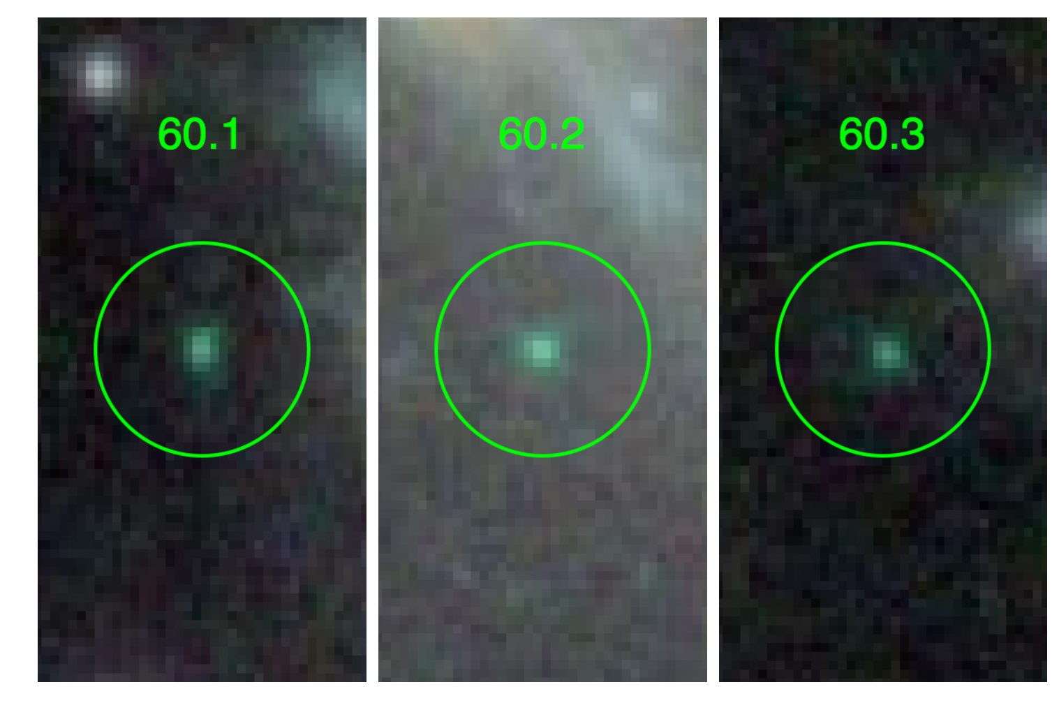
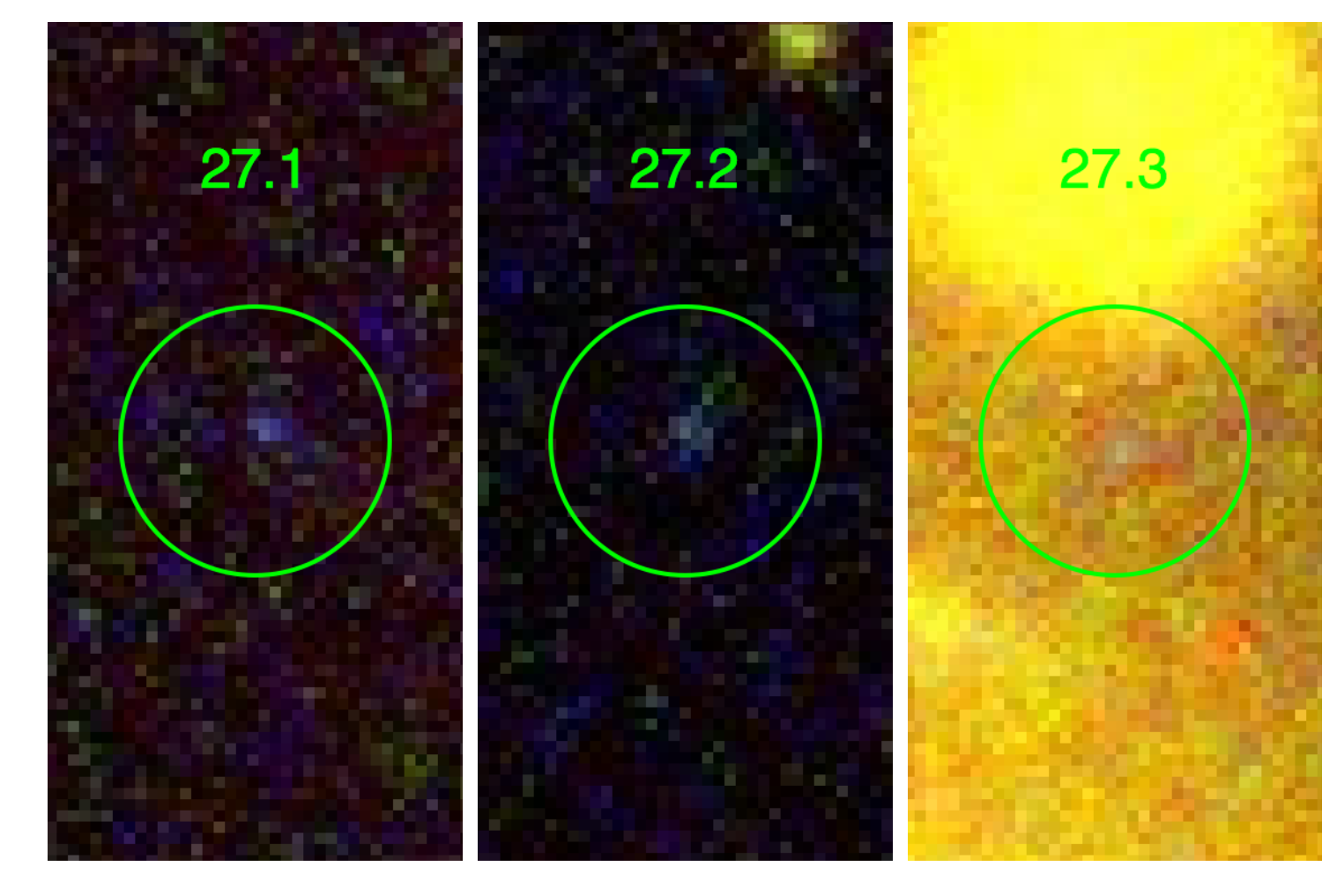
Figure 16.— Left: System 60, an example of a multiple image system whose images fulfill the morphology criteria, all three of which receive maximum grades ($M$) of 8. The images all possess the same point-like morphology and have similar surface brightnesses. This multiple image system is discovered for the first time in this work. Unfortunately, the photometric redshifts for this system were not reliable, so we could not use the image system in the lens model. The RGB image for system 60 is made from a combination of frames: F105W, F125W and F160W, with a pixel scale of 60 milli-arcseconds. Right: System 27, a multiple image system whose images fail to fulfill the color/morphology criteria due to poor morphology grades. All three images receive a morphology grade of 5. Both inspectors independently gave the images a low grade because they were too faint to discern any shareable features. The color scale is the same for all three images, showing the severe foreground contamination due to the ICL in image 27.3. Without spectroscopic redshifts and morphological details, there is no assurance that these images are of the same source other than their colors, which are largely uncertain due to the extreme faintness of the images. The RGB image for system 27 is made from a combination of frames: F435W, F814W and F125W, with a pixel scale of 60 milli-arcseconds. Out of all possible RGB combinations of HST images, the images are most discernible in this one. In both system 60 and system 27, the radius of the green circles is 0.72 arcseconds.

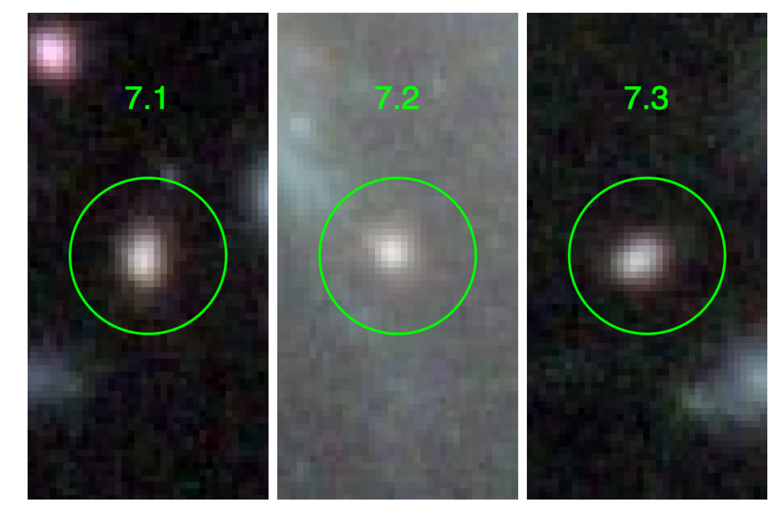
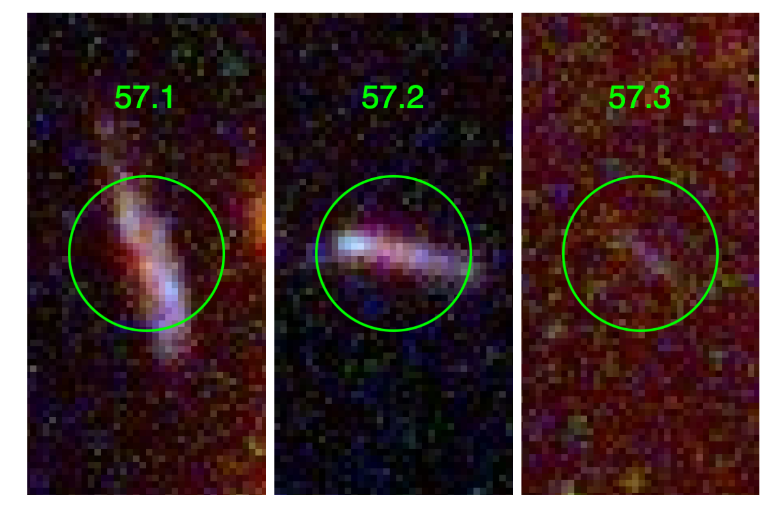
Figure 17.— Left: System 7, an example of a multiple image system whose images receive high morphology grades ($M$) of 8, 7 and 8, respectively. The RGB image for system 7 is made from a combination of frames: F105W, F125W and F160W. Right: System 57, a multiple image system that we can rule out due to an impossible lensing configuration, for which $M=0$ is assigned for all images. The proposed images are in a naked-cusp configuration and should all therefore have similar magnification. 57.3 is barely detected, yet 57.1 and 57.2 are detected at high S/N, thus invalidating the system. If 57.3 were simply misidentified, there should still be a counter-image with the same color, similar magnification and elongation as 57.1 and 57.2 nearby 57.3. We find no such counter-image. There may be another lensing configuration in which 57.1 and 57.2 are indeed multiple images of the same source, in which case there may be additional counter-images elsewhere in the cluster field that have yet to be found. The RGB image for system 57 is made from a combination of frames: F435W, F606W and F105W. In both systems 7 and 57, the radius of the green circles is 0.72 arcseconds.

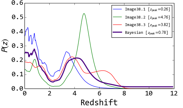
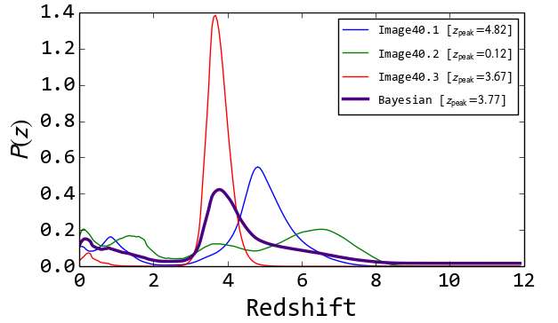
Figure 18.— Two examples of arc systems that we exclude from the lens model due to poorly-constrained redshifts. Shown are the photometric redshift probability density functions, $P(z)$, for the individual images (blue, green, red) along with a combined $P(z)$ obtained via hierarchical Bayesian modeling (purple). Left System 38 is excluded because it is bimodal with comparable probabilities under each peak. Right System 40 is excluded because the individual photometric redshifts of images 40.1, 40.2 and 40.3 are in significant disagreement.

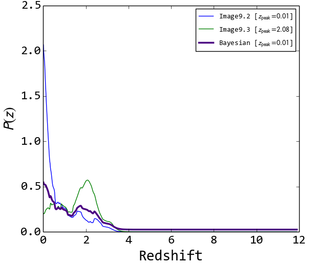
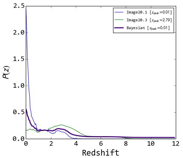
Figure 19.— Two examples of arc systems that we exclude from the lens model due to a peak in the combined Bayesian redshift below the cluster redshift of Abell 2744, $z=0.308$. Left System 9. The $P(z)$ for image 9.1 is not shown because the object is flagged as contaminated. Right System 20. Likewise, $P(z)$ for image 20.2 is not shown because the object is flagged as contaminated.

References

- Atek et al. (2014) Atek, H., Richard, J., Kneib, J.-P., et al. 2014, ApJ, 786, 60
- Atek et al. (2015) —. 2015, ApJ, 800, 18
- Bayliss et al. (2014) Bayliss, M. B., Rigby, J. R., Sharon, K., et al. 2014, ApJ, 790, 144
- Bell & de Jong (2001) Bell, E. F., & de Jong, R. S. 2001, ApJ, 550, 212
- Bertin & Arnouts (1996) Bertin, E., & Arnouts, S. 1996, Astronomy and Astrophysics Supplement, 117, 393
- Bradač et al. (2012) Bradač, M., Vanzella, E., Hall, N., et al. 2012, The Astrophysical Journal Letters, 755, L7
- Bradač et al. (2005) Bradač, M., Erben, T., Schneider, P., et al. 2005, A&A, 437, 49
- Bradač et al. (2006) Bradač, M., Clowe, D., Gonzalez, A. H., et al. 2006, ApJ, 652, 937
- Bradač et al. (2009) Bradač, M., Treu, T., Applegate, D., et al. 2009, ApJ, 706, 1201
- Bradač et al. (2014) Bradač, M., Ryan, R., Casertano, S., et al. 2014, ApJ, 785, 108
- Brammer et al. (2014) Brammer, G. B., Pirzkal, N., McCullough, P. R., & MacKenty, J. W. 2014, STScI IRS
- Brammer et al. (2008) Brammer, G. B., van Dokkum, P. G., & Coppi, P. 2008, The Astrophysical Journal, 686, 1503
- Brammer et al. (2013) Brammer, G. B., van Dokkum, P. G., Illingworth, G. D., et al. 2013, The Astrophysical Journal Letters, 765, L2
- Brammer et al. (2012) Brammer, G. B., van Dokkum, P. G., Franx, M., et al. 2012, The Astrophysical Journal Supplement, 200, 13
- Clowe et al. (2006) Clowe, D., Bradač, M., Gonzalez, A. H., et al. 2006, ApJ, 648, L109
- Coe et al. (2015) Coe, D., Bradley, L., & Zitrin, A. 2015, ApJ, 800, 84
- Dahlen et al. (2013) Dahlen, T., Mobasher, B., Faber, S. M., et al. 2013, The Astrophysical Journal, 775, 93
- Ferguson et al. (2000) Ferguson, H. C., Dickinson, M., & Williams, R. 2000, Annu. Rev. Astro. Astrophys., 38, 667
- Gavazzi et al. (2007) Gavazzi, R., Treu, T., Rhodes, J. D., et al. 2007, ApJ, 667, 176
- Gonzaga & et al. (2012) Gonzaga, S., & et al. 2012, The DrizzlePac Handbook (STScI)
- Guo et al. (2013) Guo, Y., Ferguson, H. C., Giavalisco, M., et al. 2013, ApJS, 207, 24
- Huang et al. (2015) Huang, K.-H., Bradač, M., Lemaux, B. C., et al. 2015, ArXiv e-prints, arXiv:1504.02099
- Ilbert et al. (2006) Ilbert, O., Arnouts, S., McCracken, H. J., et al. 2006, A&A, 457, 841
- Ishigaki et al. (2015) Ishigaki, M., Kawamata, R., Ouchi, M., et al. 2015, ApJ, 799, 12
- Jauzac et al. (2014) Jauzac, M., Richard, J., Jullo, E., et al. 2014, ArXiv e-prints, arXiv:1409.8663
- Johnson et al. (2014) Johnson, T. L., Sharon, K., Bayliss, M. B., et al. 2014, ApJ, 797, 48
- Johnson et al. (2014) Johnson, T. L., Sharon, K., Bayliss, M. B., et al. 2014, The Astrophysical Journal, 797, 48
- Kempner & David (2004) Kempner, J. C., & David, L. P. 2004, MNRAS, 349, 385
- Kneib & Natarajan (2011) Kneib, J.-P., & Natarajan, P. 2011, A&A Rev., 19, 47
- Koekemoer et al. (2003) Koekemoer, A. M., Fruchter, A. S., Hook, R. N., & Hack, W. 2003, The 2002 HST Calibration Workshop : Hubble after the Installation of the ACS and the NICMOS Cooling System, 337
- Kümmel et al. (2011) Kümmel, M., Kuntschner, H., Walsh, J. R., & Bushouse, H. 2011, ST-ECF Instrument Science Report WFC3-2011-01, 1
- Lam et al. (2014) Lam, D., Broadhurst, T., Diego, J. M., et al. 2014, ApJ, 797, 98
- Laporte et al. (2015) Laporte, N., Streblyanska, A., Kim, S., et al. 2015, A&A, 575, A92
- Merten et al. (2011) Merten, J., Coe, D., Dupke, R., et al. 2011, MNRAS, 417, 333
- Merten et al. (2015) Merten, J., Meneghetti, M., Postman, M., et al. 2015, ApJ, 806, 4
- Newman et al. (2013) Newman, A. B., Treu, T., Ellis, R. S., & Sand, D. J. 2013, ApJ, 765, 25
- Oke (1974) Oke, J. B. 1974, ApJS, 27, 21
- Owers et al. (2011) Owers, M. S., Randall, S. W., Nulsen, P. E. J., et al. 2011, The Astrophysical Journal, 728, 27
- Pettini et al. (2002) Pettini, M., Rix, S. A., Steidel, C. C., et al. 2002, ApJ, 569, 742
- Postman et al. (2012) Postman, M., Coe, D., Benítez, N., et al. 2012, The Astrophysical Journal Supplement, 199, 25
- Richard et al. (2014) Richard, J., Jauzac, M., Limousin, M., et al. 2014, MNRAS, 444, 268
- Rodney et al. (2015) Rodney, S. A., Patel, B., Scolnic, D., et al. 2015, ArXiv e-prints, arXiv:1505.06211
- Ryan et al. (2014) Ryan, Jr., R. E., Gonzalez, A. H., Lemaux, B. C., et al. 2014, ApJ, 786, L4
- Salpeter (1955) Salpeter, E. E. 1955, ApJ, 121, 161
- Sand et al. (2008) Sand, D. J., Treu, T., Ellis, R. S., Smith, G. P., & Kneib, J. 2008, ApJ, 674, 711
- Sharon et al. (2014) Sharon, K., Gladders, M. D., Rigby, J. R., et al. 2014, ApJ, 795, 50
- Shirazi et al. (2014) Shirazi, M., Vegetti, S., Nesvadba, N., et al. 2014, MNRAS, 440, 2201
- Treu et al. (2015) Treu, T., Schmidt, K. B., Bradač, M., et al. 2015, apJ, submitted.
- Williams et al. (1996) Williams, R. E., Blacker, B., Dickinson, M., et al. 1996, AJ, 112, 1335
- Yee et al. (1996) Yee, H. K. C., Ellingson, E., Bechtold, J., Carlberg, R. G., & Cuillandre, J.-C. 1996, AJ, 111, 1783
- Zitrin et al. (2009) Zitrin, A., Broadhurst, T., Umetsu, K., et al. 2009, MNRAS, 396, 1985
- Zitrin et al. (2014) Zitrin, A., Zheng, W., Broadhurst, T., et al. 2014, ApJ, 793, L12