Time-of-flight images of Mott insulators in the Hofstadter-Bose-Hubbard model

Abstract

We analyze the momentum distribution function and its artificial-gauge-field dependence for the Mott insulator phases of the Hofstadter-Bose-Hubbard model. By benchmarking the results of the random-phase approximation (RPA) approach against those of the strong-coupling expansion (SCE) for the Landau and symmetric gauges, we find pronounced corrections to the former results, which is a clear manifestation of the critical role played by quantum fluctuations in two dimensions.

Introduction: The momentum distribution function $n(\mathbf{k})$ of atoms, which is defined as the Fourier transform of the one-body density matrix, can be directly measured in cold-atom systems by time-of-flight absorption imaging of freely expanding gas lewenstein07 ; bloch08 ; giorgini08 . Since these systems are extremely dilute, the atom-atom interactions are negligible during such an expansion, and the position of atoms at time $\tau$ are strongly correlated with their velocity distribution at the moment of release from the trap, i.e., $\mathbf{r}=\hbar\mathbf{k}\tau/m$ with $\hbar$ the Planck constant and $m$ the atomic mass. Therefore, the $n(\mathbf{k})$ of atoms has not only been the easiest observable to measure but also been routinely used for probing distinct phases of matter in atomic systems.

In addition, followed by the recent advances in creating artificial gauge fields in atomic systems dalibard11 ; galitski13 , there has been growing interest in first the realization of the Hofstadter-type lattice Hamiltonians and then the detection of the resultant many-body phases garcia12 ; struck12 ; aidelsburger13 ; miyake13 ; kennedy15 . For instance, the MIT group has in their latest preprint measured the $n(\mathbf{k})$ of atoms in the superfluid (SF) phase kennedy15 , revealing both the reduced symmetry of their specific gauge field and the resultant degeneracy of the ground state leblanc15 . There is no doubt that such a capacity to tune strong gauge fields together with strong interactions paves ultimately the way for creating and observing uncharted many-body phases and transitions in between, one of the immediate candidates of which is the renowned SF-MI transition lewenstein07 ; bloch08 .

Motivated by these recent works, in this brief paper, we study $n(\mathbf{k})$ of atoms for the MI phases of the Hofstadter-Bose-Hubbard model on a square lattice. For this purpose, we compare the results of RPA and SCE approaches for the Landau and symmetric gauges, and find substantial corrections to the former results depending strongly on the specified gauge.

Hamiltonian and Phase Diagram: These results are obtained for the following Hamiltonian

$$H=-\sum_{ij}t_{ij}c_{i}^{\dagger}c_{j}+\frac{U}{2}\sum_{i}\widehat{n}_{i}(\widehat{n}_{i}-1)-\mu\sum_{i}\widehat{n}_{i},$$ (1)

where the hopping parameter $t_{ij}=te^{i\theta_{ij}}$ connects nearest-neighbor sites with phase factor $\theta_{ij}$ taking the gauge fields into account, $c_{i}^{\dagger}$ ($c_{i}$) creates (annihilates) a boson on site $i$, the boson-boson interaction is on-site and repulsive $U\geq 0$, $\widehat{n}_{i}=c_{i}^{\dagger}c_{i}$ is the number operator, and $\mu\geq 0$ is the chemical potential. In this paper, we compare the results of the usual $(A)$ no-gauge limit, where $\theta_{ij}=0$ for all hoppings; with those of $(B)$ Landau gauge, where $\theta_{ij}=2\pi\phi u$ for $(u,v)$ to $(u,v+1)$ and $0$ for $(u,v)$ to $(u+1,v)$ hoppings; $(C)$ symmetric gauge, where $\theta_{ij}=\pi\phi u$ for $(u,v)$ to $(u,v+1)$ and $-\pi\phi v$ for $(u,v)$ to $(u+1,v)$ hoppings; and $(D)$ MIT gauge kennedy15 , where $\theta_{ij}=2\pi\phi(u+v)$ for $(u,v)$ to $(u,v+1)$ and $0$ for $(u,v)$ to $(u+1,v)$ hoppings. Here, $(u,v)$ corresponds to the Cartesian coordinates of site $i$, and $\theta_{ij}$ are chosen such that the magnetic flux $\phi=p/q$ is the same for all gauges, where $p$ and $q$ are co-prime numbers with $p\leq q$.

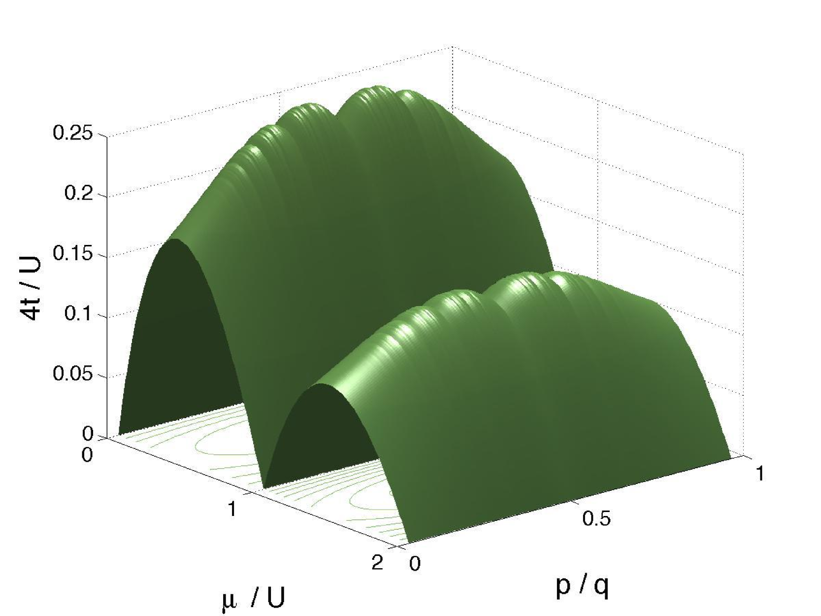
Figure 1: (Color online) The ground-state phase diagram is shown as a function of chemical potential $\mu$, magnetic flux $\phi=p/q$ and hopping strength $4t$.

In the atomic ($t=0$) limit, since $H$ commutes with $\widehat{n}_{i}$, the thermal average $n_{i}=\langle\widehat{n}_{i}\rangle$ is such that the ground-state energy is minimised for a given $\mu$, leading to a uniform occupation ($n_{i}=n$) of bosons thanks to the translational invariance of $H$. When $U=0$ and $\mu=0$, the spectrum of $H$ corresponds to the celebrated Hofstadter butterfly hofstadter76 ; kohmoto89 . It is also very well-known that the range of $\mu$ about which the ground state is a MI with an integer occupation $n$ decreases as a function of increasing $t/U$, and depending on $n$ and $\phi$, the MIs disappear at a critical value of $t/U$, beyond which the system becomes a SF niemeyer99 . For instance, the qualitative phase diagram of $H$ can be obtained within the mean-field approximation, e.g., the decoupling or variational Gutzwiller techniques, leading to umucalilar07 ; goldbaum09 ; iskina

$$\frac{1}{\epsilon^{pq}}=\frac{n+1}{Un-\mu}-\frac{n}{U(n-1)-\mu}$$ (2)

at zero temperature for the MI-SF phase transition boundary, where $n\geq 0$ is an integer number. Here, $\epsilon^{pq}$ is the minimal eigenvalue of the hopping matrix $\sum_{j}(-t_{ij})f_{j}=\epsilon^{pq}f_{i}$ and it corresponds to the maximal single-particle kinetic energy of the Hofstadter butterfly, e.g., $\epsilon^{0}=4t$ when $\phi=0$. Since the effects of $\theta_{ij}$ enter Eq. (2) through its dependence on $\epsilon^{pq}$, the mean-field phase boundary is clearly independent of the gauge, which is simply because only the position in the magnetic Brillouin zone but not the value of $\epsilon^{pq}$ depends on the gauge. However, this is not the case for the SF properties which are gauge dependent within the mean-field approaches.

In Fig. 1, we show the ground-state phase diagram as a function of $\mu$, $\phi=p/q$ and $4t$, which is obtained by solving Eq. (2) together with the Harper’s equation. Both the symmetry around $p/q=1/2$ and the intriguing structure of the MI-SF phase transition boundary are due to the dependence of $\epsilon^{pq}$ on $\phi$ hofstadter76 ; kohmoto89 . In addition, the incompressible (compressible) MI (SF) phase grows (shrinks) when $\phi$ increases from $0$, a consequence of which is due to the localizing effects of magnetic flux on particles, and all of these results are in agreement with earlier findings niemeyer99 ; umucalilar07 ; goldbaum09 ; iskina . Having introduced the model Hamiltonian and reviewed its phase diagram, next we are ready to discuss the momentum distribution of bosons for the MIs.

Momentum Distribution: As discussed in the Introduction, the $n(\mathbf{k})$ of atoms corresponds to the Fourier transform of the one-body density matrix, and it is given by freericks09 ; iskin09 ; moller10 ; sinha11

$$n(\mathbf{k})=\frac{|w(\mathbf{k})|^{2}}{M}\sum_{jj^{\prime}}\langle c_{j^{\prime}}^{\dagger}c_{j}\rangle e^{i\mathbf{k}\cdot(\mathbf{r_{j^{\prime}}}-\mathbf{r_{j}})},$$ (3)

where $M$ is the number of sites and $\mathbf{r_{j}}=(ua,va)$ is the position of site $j$ with $a$ the lattice spacing. In the following, we set the Fourier transform of the Wannier function $w(\mathbf{k})$ to $1$, since it depends on the particular optical lattice potential and has nothing to do with our $H$.

In this paper, we calculate $n(\mathbf{k})$ for the MIs using two approaches: $(I)$ RPA sinha11 ; iskin09 and $(II)$ SCE in $t/U$ freericks09 ; iskin09 . We emphasize that while the result of the RPA approach corresponds to the exact $n(\mathbf{k})$ only in the limit of infinite dimensions and zero magnetic flux, the results of the SCE approach are exact in two dimensions for the specified gauges up to the given order in $t/U$.

(I) Random-Phase Approximation: In the RPA approach sinha11 ; iskin09 , since the thermal averages of products of operators are replaced by the product of their thermal averages, the fluctuations are not fully taken into account. After a lengthy but straightforward algebra, one finds

$$n_{\textrm{RPA}}^{pq}(\mathbf{k})=\frac{1}{2q}\sum_{\ell=0}^{q-1}\frac{\varepsilon_{\ell}^{pq}(\mathbf{k})+\widetilde{U}}{\sqrt{\left[\varepsilon_{\ell}^{pq}(\mathbf{k})\right]^{2}+2\widetilde{U}\varepsilon_{\ell}^{pq}(\mathbf{k})+U^{2}}}-\frac{1}{2}$$ (4)

for a MI with $n$ bosons per site at zero temperature, where $\widetilde{U}=U(2n+1)$ and $\varepsilon_{\ell}^{pq}(\mathbf{k})$ is the energy dispersion of a single particle in the $\ell$th Hofstadter band. Note that the form of Eq. (4) is exactly the same as the usual Bose-Hubbard model, i.e., the main difference is a sum over the Hofstadter bands, and that it has an overall factor of $1/q$ in comparison to the one given in Ref. sinha11 . While the set of $\varepsilon_{\ell}^{pq}(\mathbf{k})$ values depends only on $\phi$ and lattice geometry, their corresponding positions in the 1st magnetic Brillouin zone, and therefore $n(\mathbf{k})$, are gauge dependent moller10 ; sinha11 . For instance, $n(\mathbf{k})$ exhibits $q$ peaks as a function of $\mathbf{k}$, and only the number $q$ but not the positions are controlled by $\phi$. Note that $\epsilon^{pq}\equiv\max\{\varepsilon_{\ell}^{pq}(\mathbf{k})\}$ in Eq. (2) which is also a gauge-independent quantity as remarked above. In particular, when $\phi=0$, a $d$-dimensional hypercubic lattice gives rise to a single band with dispersion $\varepsilon^{0}(\mathbf{k})=-2t\sum_{k_{i},i=1}^{d}\cos(k_{i}a)$, and it is already established that $n_{\textrm{RPA}}^{0}(\mathbf{k})$ becomes exact as $d\to\infty$ while keeping $dt$ fixed freericks09 ; iskin09 .

To compare Eq. (4) with our exact results of the SCE approach derived below, let us expand $n_{\textrm{RPA}}^{pq}(\mathbf{k})$ in a power series up to $3$rd order in $t/U$, leading to

$$n_{\textrm{RPA}}^{pq}(\mathbf{k}) =n-\frac{2n(n+1)}{qU}\sum_{\ell=0}^{q-1}\varepsilon_{\ell}^{pq}(\mathbf{k})$$

$$+\frac{3n(n+1)(2n+1)}{qU^{2}}\sum_{\ell=0}^{q-1}\left[\varepsilon_{\ell}^{pq}(\mathbf{k})\right]^{2}$$

$$-\frac{4n(n+1)(5n^{2}+5n+1)}{qU^{3}}\sum_{\ell=0}^{q-1}\left[\varepsilon_{\ell}^{pq}(\mathbf{k})\right]^{3}.$$ (5)

For a given $\phi$, the sums over Hofstadter bands can be easily evaluated for a given gauge by noting $\sum_{\ell=0}^{q-1}\left[\varepsilon_{\ell}^{pq}(\mathbf{k})\right]^{s}=\textrm{Trace}\big{\{}\left[T^{pq}(\mathbf{k})\right]^{s}\big{\}},$ where $T^{pq}(\mathbf{k})$ describes the kinetic energy of a single particle in the $1$st magnetic Brillouin zone.

For instance, $T^{pq}(\mathbf{k})$ is a $q\times q$ matrix in the Landau gauge hofstadter76 ; kohmoto89

$$\begin{bmatrix}h_{0}&-te^{ik_{x}a}&0&.&-te^{-ik_{x}a}\\ -te^{-ik_{x}a}&h_{1}&-te^{ik_{x}a}&.&0\\ 0&-te^{-ik_{x}a}&h_{2}&.&.\\ .&.&.&.&-te^{ik_{x}a}\\ -te^{ik_{x}a}&0&.&-te^{-ik_{x}a}&h_{q-1}\end{bmatrix}$$ (6)

with $h_{\ell}=-2t\cos(k_{y}a+2\pi\phi\ell)$, for which the $s=1$ trace equals to $-2t[\cos(k_{x}a)+\cos(k_{y}a)]$ when $(p,q)=(1,1)$ and it vanishes for $q>1$; the $s=2$ trace equals to $4t^{2}\left[\cos(k_{x}a)+\cos(k_{y}a)\right]^{2}$ when $(p,q)=(1,1)$, to $8t^{2}\left[\cos^{2}(k_{x}a)+\cos^{2}(k_{y}a)\right]$ when $(p,q)=(1,2)$ and to $4qt^{2}$ for $q>2$; and lastly the $s=3$ trace equals to $-8t^{3}\left[\cos(k_{x}a)+\cos(k_{y}a)\right]^{3}$ when $(p,q)=(1,1)$ and to $-6t^{3}\left[\cos(3k_{x}a)+\cos(3k_{y}a)\right]$ when $q=3$, but it vanishes for $q>3$. Thus, Eq. (Time-of-flight images of Mott insulators in the Hofstadter-Bose-Hubbard model) reduces to

$$n_{\textrm{RPA}}^{11}(\mathbf{k}) =n+\frac{4n(n+1)}{(U/t)}[\cos(k_{x}a)+\cos(k_{y}a)]+\frac{12n(n+1)(2n+1)}{(U/t)^{2}}[\cos(k_{x}a)+\cos(k_{y}a)]^{2}$$

$$+\frac{32n(n+1)(5n^{2}+5n+1)}{(U/t)^{3}}[\cos(k_{x}a)+\cos(k_{y}a)]^{3},$$ (7)

$$n_{\textrm{RPA}}^{12}(\mathbf{k}) =n+\frac{6n(n+1)(2n+1)}{(U/t)^{2}}[\cos(2k_{x}a)+\cos(2k_{y}a)+2]+\mathcal{O}(t/U)^{4},$$ (8)

$$n_{\textrm{RPA}}^{p3}(\mathbf{k}) =n+\frac{12n(n+1)(2n+1)}{(U/t)^{2}}+\frac{8n(n+1)(5n^{2}+5n+1)}{(U/t)^{3}}[\cos(3k_{x}a)+\cos(3k_{y}a)],$$ (9)

$$n_{\textrm{RPA}}^{p,q>3}(\mathbf{k}) =n+\frac{12n(n+1)(2n+1)}{(U/t)^{2}}+\mathcal{O}(t/U)^{4}.$$ (10)

Equations (Time-of-flight images of Mott insulators in the Hofstadter-Bose-Hubbard model-10) clearly show that the first $\mathbf{k}$ dependence of $n_{\textrm{RPA}}^{pq}(\mathbf{k})$ arises at the $q$th order in $t/U$. More importantly, we note that Eqs. (Time-of-flight images of Mott insulators in the Hofstadter-Bose-Hubbard model-10) are symmetric in $k_{x}$ and $k_{y}$ even though the spatial symmetry between $x$ and $y$ directions is explicitly broken by the Landau gauge. Note also that Eq. (Time-of-flight images of Mott insulators in the Hofstadter-Bose-Hubbard model) coincides with that of the $\phi=0$ result since $\varepsilon_{\ell}^{pq}(\mathbf{k})$ is a periodic function of $\phi$ with a period of $1$ hofstadter76 ; kohmoto89 . Unlike the $\phi=0$ case for which the RPA approach captures the essential features of $n^{0}(\mathbf{k})$ even in finite dimensions freericks09 ; iskin09 , next we use the SCE approach and show that the corrections to $n_{\textrm{RPA}}^{pq}(\mathbf{k})$ are quite dramatic in the presence of gauge fields in two dimensions.

(II) Strong-Coupling Expansion: In the SCE approach freericks09 ; iskin09 , the wave function of MIs is achieved via a many-body perturbation theory in the kinetic energy term up to $3$rd order in $t/U$. In principle, one can apply the perturbation theory on the $0$th-order wave function $|\Psi_{\rm MI}^{(0)}\rangle=\prod_{j=1}^{M}\left(c_{j}^{\dagger}\right)^{n}|0\rangle/\sqrt{n!},$ where $|0\rangle$ is the vacuum state, and calculate $|\Psi_{\rm MI}\rangle$ up to any desired order. However, since the number of intermediate states increases dramatically, here we perform this expansion only up to $3$rd order in $t/U$, and obtain $|\Psi_{\rm MI}\rangle=|\psi_{\rm MI}\rangle/A$ where

$$|\psi_{\rm MI}\rangle =|\Psi_{\rm MI}^{(0)}\rangle+\sum_{m^{\prime}}\frac{V_{m^{\prime}0}}{E_{0m^{\prime}}}|m^{\prime}\rangle+\sum_{m^{\prime}m^{\prime\prime}}\frac{V_{m^{\prime\prime}m^{\prime}}V_{m^{\prime}0}}{E_{0m^{\prime\prime}}E_{0m^{\prime}}}|m^{\prime\prime}\rangle$$

$$+\sum_{m^{\prime}m^{\prime\prime}m^{\prime\prime\prime}}\frac{V_{m^{\prime\prime\prime}m^{\prime\prime}}V_{m^{\prime\prime}m^{\prime}}V_{m^{\prime}0}}{E_{0m^{\prime\prime\prime}}E_{0m^{\prime\prime}}E_{0m^{\prime}}}|m^{\prime\prime\prime}\rangle+\cdots$$ (11)

is the unnormalized wave function which needs to be divided by a proper normalization coefficient $A$ in order to get the correct order of perturbation. Here, $V_{m^{\prime}0}=-\sum_{jj^{\prime}}t_{jj^{\prime}}\langle m^{\prime}|c_{j}^{\dagger}c_{j^{\prime}}|\Psi_{\rm MI}^{(0)}\rangle$ connects the $1$st-order intermediate states $|m^{\prime}\rangle$ to $|\Psi_{\rm MI}^{(0)}\rangle$, $E_{0m^{\prime}}=E_{\rm MI}^{(0)}-E_{m^{\prime}}^{(0)}$ is their $0$th-order energy difference, and $|m^{\prime\prime}\rangle$ and $|m^{\prime\prime\prime}\rangle$ are respectively the $2$nd and $3$rd-order intermediate states. Note that while $|\Psi_{\rm MI}^{(0)}\rangle$ and $|m^{\prime}\rangle$, $|m^{\prime}\rangle$ and $|m^{\prime\prime}\rangle$, and $|m^{\prime\prime}\rangle$ and $|m^{\prime\prime\prime}\rangle$ states are connected to each other with a single hopping, $|m^{\prime\prime}\rangle$ and $|m^{\prime\prime\prime}\rangle$ states must be different from the $|\Psi_{\rm MI}^{(0)}\rangle$ state. Therefore, the normalization condition $\langle\Psi_{\rm MI}|\Psi_{\rm MI}\rangle=1$ gives $A^{2}=1+4n(n+1)Mt^{2}/U^{2}+O(t/U)^{4},$ which has vanishing $1$st and $3$rd order terms.

After a very lengthy and tedious algebra, one finds

$$\langle\Psi_{\rm MI}|a_{j^{\prime}}^{\dagger} a_{j}|\Psi_{\rm MI}\rangle=n\delta_{jj^{\prime}}+\frac{2n(n+1)}{U}t_{jj^{\prime}}$$

$$+\frac{3n(n+1)(2n+1)}{U^{2}}\left(\sum_{j_{1}}t_{jj_{1}}t_{j_{1}j^{\prime}}-4t^{2}\delta_{jj^{\prime}}\right)$$

$$+\frac{4n(n+1)(5n^{2}+5n+1)}{U^{3}}\sum_{j_{1}j_{2}}t_{jj_{2}}t_{j_{2}j_{1}}t_{j_{1}j^{\prime}}$$

$$-\frac{n(n+1)(131n^{2}+131n+26)}{U^{3}}t^{2}t_{jj^{\prime}}$$ (12)

for a square lattice with nearest-neighbor hopping at zero temperature. We note in Eq. (Time-of-flight images of Mott insulators in the Hofstadter-Bose-Hubbard model) that the $2$ terms that are explicitly proportional to $t^{2}$ are finite-$d$ corrections, including the $2$nd term in the $2$nd line and the $4$th line, as they vanish in the $d\to\infty$ limit while keeping $dt$ fixed. Since Eq. (Time-of-flight images of Mott insulators in the Hofstadter-Bose-Hubbard model) is derived exactly using a generic hopping matrix $t_{ij}$, we are ready to benchmark it against the results of the RPA approach for a number of specified gauges. For this purpose, we make use of the following identities: the sum $\sum_{\ell=0}^{q-1}\cos(\alpha-2n\pi\phi\ell)$ equals to $q\cos(\alpha)$ when $q=n$ and it vanishes for $q>n$; the sum $\sum_{\ell=0}^{q-1}\cos^{2}(\alpha-2\pi\phi\ell)$ equals to $q\cos^{2}(\alpha)$ when $(p,q)=\{(1,1),(1,2)\}$ and $q/2$ for $q>2$; and the sum $\sum_{\ell=0}^{q-1}\cos^{3}(\alpha-2\pi\phi\ell)$ equals to $\cos^{3}(\alpha)$ when $(p,q)=(1,1)$ and to $3\cos(3\alpha)/4$ when $q=3$, but it vanishes for $(p,q)=(1,2)$ or $q>3$.

(II-A) No-Gauge Limit: Setting $\theta_{ij}=0$ for all hoppings in Eq. (Time-of-flight images of Mott insulators in the Hofstadter-Bose-Hubbard model), we obtain

$$n^{0}(\mathbf{k}) =n-\frac{2n(n+1)}{U}\varepsilon^{0}(\mathbf{k})$$

$$+\frac{3n(n+1)(2n+1)}{U^{2}}\{[\varepsilon^{0}(\mathbf{k})]^{2}-4t^{2}\}$$

$$-\frac{4n(n+1)(5n^{2}+5n+1)}{U^{3}}[\varepsilon^{0}(\mathbf{k})]^{3}$$

$$+\frac{n(n+1)(131n^{2}+131n+26)}{U^{3}}t^{2}\varepsilon^{0}(\mathbf{k}),$$ (13)

where $\varepsilon^{0}(\mathbf{k})=-2t\left[\cos(k_{x}a)+\cos(k_{y}a)\right]$ is the usual dispersion relation for a square lattice. Since the two terms that are explicitly proportional to $t^{2}$ are finite-$d$ corrections, they are not captured by the result of the RPA approach that is given in Eq. (Time-of-flight images of Mott insulators in the Hofstadter-Bose-Hubbard model).

(II-B) Landau Gauge: On the other hand, setting $\theta_{ij}=2\pi\phi u$ for $(u,v)$ to $(u,v+1)$ and $0$ for $(u,v)$ to $(u+1,v)$ hoppings in Eq. (Time-of-flight images of Mott insulators in the Hofstadter-Bose-Hubbard model), we obtain

$$n_{\textrm{L}}^{11}(\mathbf{k}) =n+\frac{4n(n+1)}{(U/t)}[\cos(k_{x}a)+\cos(k_{y}a)]+\frac{12n(n+1)(2n+1)}{(U/t)^{2}}\big{\{}[\cos(k_{x}a)+\cos(k_{y}a)]^{2}-1\big{\}}$$ (14)

$$+\frac{32n(n+1)(5n^{2}+5n+1)}{(U/t)^{3}}[\cos(k_{x}a)+\cos(k_{y}a)]^{3}-\frac{2n(n+1)(131n^{2}+131n+26)}{(U/t)^{3}}[\cos(k_{x}a)+\cos(k_{y}a)],$$

$$n_{\textrm{L}}^{12}(\mathbf{k}) =n+\frac{4n(n+1)}{(U/t)}\cos(k_{x}a)+\frac{6n(n+1)(2n+1)}{(U/t)^{2}}[\cos(2k_{x}a)+\cos(2k_{y}a)]$$ (15)

$$+\frac{32n(n+1)(5n^{2}+5n+1)}{(U/t)^{3}}\cos(k_{x}a)[\cos^{2}(k_{x}a)+\cos^{2}(k_{y}a)]-\frac{2n(n+1)(131n^{2}+131n+26)}{(U/t)^{3}}\cos(k_{x}a),$$

$$n_{\textrm{L}}^{p3}(\mathbf{k}) =n+\frac{4n(n+1)}{(U/t)}\cos(k_{x}a)+\frac{6n(n+1)(2n+1)}{(U/t)^{2}}\cos(2k_{x}a)$$ (16)

$$+\frac{8n(n+1)(5n^{2}+5n+1)}{(U/t)^{3}}[\cos(3k_{x}a)+\cos(3k_{y}a)+6\cos(k_{x}a)]-\frac{2n(n+1)(131n^{2}+131n+26)}{(U/t)^{3}}\cos(k_{x}a),$$

$$n_{\textrm{L}}^{p,q>3}(\mathbf{k}) =n+\frac{4n(n+1)}{(U/t)}\cos(k_{x}a)+\frac{6n(n+1)(2n+1)}{(U/t)^{2}}\cos(2k_{x}a)$$ (17)

$$+\frac{8n(n+1)(5n^{2}+5n+1)}{(U/t)^{3}}\big{\{}\cos(3k_{x}a)+[7+2\cos(2\pi p/q)]\cos(k_{x}a)\big{\}}-\frac{2n(n+1)(131n^{2}+131n+26)}{(U/t)^{3}}\cos(k_{x}a).$$

Note that Eq. (14) exactly coincides with Eq. (Time-of-flight images of Mott insulators in the Hofstadter-Bose-Hubbard model) since $\phi=1$ and $0$ are equivalent in this gauge. We also note that, unlike the results of the RPA approach that are given in Eqs. (Time-of-flight images of Mott insulators in the Hofstadter-Bose-Hubbard model-10), these exact results are not symmetric in $k_{x}$ and $k_{y}$, showing that it is only the first $k_{y}$ dependence that arises at the $q$th order in $t/U$. This is not surprising because while the one-body correlation operator $c_{j^{\prime}}^{\dagger}c_{j}$ connects $|\Psi_{\rm MI}\rangle$ to itself at the $1$st order in $x$ direction, the connection is established at the $q$th order in $y$ direction due to the presence of $2\pi\phi u$. In addition, on top of the RPA contributions, Eqs. (14-17) contain various other terms, showing that the finite-$d$ corrections are quite substantial in the presence of gauge fields in two dimensions footnote . Thus, one of our main conclusions in this paper is that the mismatch between the results of RPA and SCE approaches grows so dramatically as $q$ increases from $1$ that the former approach fails to reproduce any of the exact terms up to $3$rd order in $t/U$ for $q>3$.

(II-C) Symmetric Gauge: Similarly, setting $\theta_{ij}=\pi\phi u$ for $(u,v)$ to $(u,v+1)$ and $-\pi\phi v$ for $(u,v)$ to $(u+1,v)$ hoppings in Eq. (Time-of-flight images of Mott insulators in the Hofstadter-Bose-Hubbard model), we obtain

$$n_{\textrm{S}}^{11}(\mathbf{k}) =n+\frac{12n(n+1)(2n+1)}{(U/t)^{2}}\big{\{}[\cos(k_{x}a)$$

$$+\cos(k_{y}a)]^{2}-1\big{\}}+\mathcal{O}(t/U)^{4},$$ (18)

$$n_{\textrm{S}}^{p,q>1}(\mathbf{k}) =n+\mathcal{O}(t/U)^{4}.$$ (19)

Note that Eq. (Time-of-flight images of Mott insulators in the Hofstadter-Bose-Hubbard model) does not reproduce Eq. (Time-of-flight images of Mott insulators in the Hofstadter-Bose-Hubbard model) since $\phi=1$ and $0$ are not equivalent in this gauge. We also note that, unlike the results of the SCE approach for the Landau gauge that are given in Eqs. (14-17), here the $\mathbf{k}$ dependence is not only symmetric in $k_{x}$ and $k_{y}$, thanks to the spatial symmetry between $x$ and $y$ directions, but also the first $\mathbf{k}$ dependence arises at the $2q$th order in $t/U$. This is also not surprising because the one-body correlation operator $c_{j^{\prime}}^{\dagger}c_{j}$ connects $|\Psi_{\rm MI}\rangle$ to itself at the $2q$th order in both directions due to the presence of $\pi\phi u$. In addition, the $\mathbf{k}$-independent $2$nd order term in Eq. (18) is a finite-$d$ correction to the result of the RPA approach in this gauge. Therefore, $n_{S}^{pq}(\mathbf{k})$ becomes more and more featureless function of $\mathbf{k}$ as $q$ increases from $1$, especially deep in the MIs when $t/U$ is very small.

(II-D) MIT Gauge: Lastly, setting $\theta_{ij}=2\pi\phi(u+v)$ for $(u,v)$ to $(u,v+1)$ and $0$ for $(u,v)$ to $(u+1,v)$ hoppings in Eq. (Time-of-flight images of Mott insulators in the Hofstadter-Bose-Hubbard model) leads exactly to Eqs. (14-17), and therefore, the MIT kennedy15 and Landau gauges have exactly the same $n(\mathbf{k})$.

Conclusions: To summarize, we studied the expansion images of atoms for the MI phases of the Hofstadter-Bose-Hubbard model on a square lattice. In particular, we explicitly calculated the momentum distribution function for the Landau and symmetric gauges with both RPA and SCE approaches, and found marked corrections to the former results depending strongly on the specified gauge. Such a comparison clearly manifests the importance of the critical role played by quantum fluctuations in two dimensions.

Acknowledgments: We gratefully acknowledge funding from TÜB$\dot{\mathrm{I}}$TAK Grant No. 1001-114F232.

References

• (1) M. Lewenstein, A. Sanpera, V. Ahufinger, B. Damski, A. Sen De, and U. Sen, Adv. Phy. 56, 243 (2007).
• (2) I. Bloch, J. Dalibard, and W. Zwerger, Rev. Mod. Phys. 80, 885 (2008).
• (3) S. Giorgini, L. P. Pitaevskii, and S. Stringari, Rev. Mod. Phys. 80, 1215 (2008).
• (4) J. Dalibard, F. Gerbier, G. Juzelinas, and P. Γ–hberg, Rev. Mod. Phys. 83, 1523 (2011).
• (5) V. Galitski and I. B. Spielman, Nature 494, 49 (2013).
• (6) K. JimΓ©nez-GarcΓ­a, L. J. LeBlanc, R. A. Williams, M. C. Beeler, A. R. Perry, and I. B. Spielman, Phys. Rev. Lett. 108, 225303 (2012).
• (7) J. Struck, C. Γ–lschlΓ€ger, M. Weinberg, P. Hauke, J. Simonet, A. Eckardt, M. Lewenstein, K. Sengstock, and P. Windpassinger, Phys. Rev. Lett. 108, 225304 (2012).
• (8) M. Aidelsburger, M. Atala, M. Lohse, J. T. Barreiro, B. Paredes, and I. Bloch, Phys. Rev. Lett. 111, 185301 (2013).
• (9) H. Miyake, G. A. Siviloglou, C. J. Kennedy, W. C. Burton, and W Ketterle, Phys. Rev. Lett. 111, 185302 (2013).
• (10) C. J. Kennedy, W. C. Burton, W. C. Chung, and W. Ketterle, arXiv:1503.08243 (2015).
• (11) See also: L. J. LeBlanc, K. JimΓ©nez-Garc a, R. A. Williams, M. C. Beeler, W. D. Phillips, and I. B. Spielman, arXiv:1502.07443 (2015) for a somewhat related work in continuum.
• (12) D. R. Hofstadter, Phys. Rev. B 14, 2239 (1976).
• (13) M. Kohmoto, Phys. Rev. B 39, 11943 (1989).
• (14) M. Niemeyer, J. K. Freericks, and H. Monien, Phys. Rev. B 60, 2357 (1999).
• (15) R. O. UmucalΔ±lar and M. Γ–. Oktel, Phys. Rev. A 76, 055601 (2007).
• (16) D. S. Goldbaum and E. J. Mueller, Phys. Rev. A 79, 021602(R) (2009).
• (17) M. Iskin, Eur. Phys. J. B 85, 76 (2012).
• (18) J. K. Freericks, H. R. Krishnamurthy, Y. Kato, N. Kawashima, and N. Trivedi, Phys. Rev. A 79, 053631 (2009).
• (19) M. Iskin and J. K. Freericks, Phys. Rev. A 80, 063610 (2009).
• (20) S. Sinha and K. Sengupta, EPL 93, 30005 (2011).
• (21) G. MΓΆller and N. R. Cooper, Phys. Rev. A 82, 063625 (2010).
• (22) We note that since the $\mathbf{k}$-independent $2$nd order RPA terms that are found in Eqs.Β (9-10) are coincidentally canceled by the finite-$d$ correction that is found in Eq.Β (Time-of-flight images of Mott insulators in the Hofstadter-Bose-Hubbard model), these terms do not appear in Eqs.Β (16-17).