Spatially discrete reaction-diffusion equations with discontinuous hysteresis

Abstract

We address the question: Why may reaction-diffusion equations with hysteretic nonlinearities become ill-posed and how to amend this? To do so, we discretize the spatial variable and obtain a lattice dynamical system with a hysteretic nonlinearity. We analyze a new mechanism that leads to appearance of a spatio-temporal pattern called rattling: the solution exhibits a propagation phenomenon different from the classical traveling wave, while the hysteretic nonlinearity, loosely speaking, takes a different value at every second spatial point, independently of the grid size. Such a dynamics indicates how one should redefine hysteresis to make the continuous problem well-posed and how the solution will then behave. In the present paper, we develop main tools for the analysis of the spatially discrete model and apply them to a prototype case. In particular, we prove that the propagation velocity is of order $at^{-1/2}$ as $t\to\infty$ and explicitly find the rate $a$.

1 Introduction

1.1 Background

Hysteresis, or, more generally, bistability, refers to a class of nonlinear phenomena which are observed in numerous real-world systems. It arises in description of ferromagnetic materials, shape-memory alloys, elasto-plastic bodies, as well as many biological, economical, and social models, see [20, 27, 8, 22, 23, 21]. The primary goal of the present paper is to analyze a new mechanism (which we call rattling) for pattern formation in spatially discrete systems of reaction-diffusion equations (lattice dynamical systems) with hysteresis. The phenomenon occurs in any space dimension, including dimension one, and persists even for scalar equations. As it is explained below, our results are relevant not only for lattice dynamical systems, but also for continuous systems with hysteresis. On the other hand, they link pattern formation mechanisms in hysteretic and bistable slow-fast systems.

Let us begin with the prototype spatially continuous problem

$$\left\{\begin{aligned} &v_{\tau}=v_{xx}+{\mathcal{H}}(v),\quad x\in(-1,1),\ \tau>0,\\ &v(x,0)=\varphi(x),\quad x\in(-1,1),\end{aligned}\right.$$ (1.1)

supplemented with, e.g., Neumann boundary conditions. Here ${\mathcal{H}}(\cdot)$ is the simplest hysteresis operator, namely, the non-ideal relay or bistable switch, see Fig. 1.1.a and the (slightly modified) rigorous definition in Section 2.

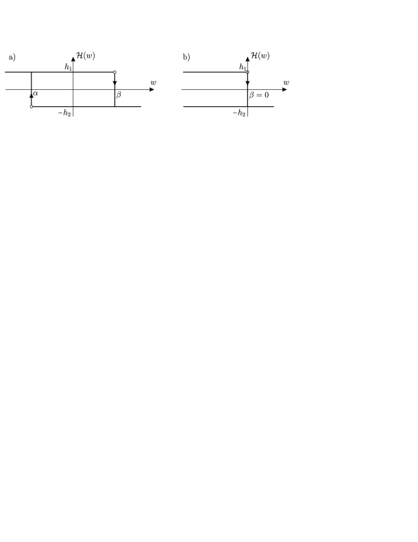
Figure 1.1: Hysteresis a) with thresholds $\alpha<\beta$. b) with thresholds $\alpha=-\infty$ and $\beta=0$.

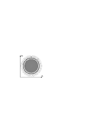
Figure 1.2: Bacteria density at end of experiment.

Hysteresis is defined by two thresholds $\alpha<\beta$ and two values $h_{1},-h_{2}\in\mathbb{R}$ (in what follows, we are interested in the case $h_{1}>0\geq-h_{2}$). Given a continuous input function $w(\tau)$, its output ${\mathcal{H}}(w)(\tau)$ remains constant unless the input achieves the lower threshold $\alpha$ or the upper threshold $\beta$. In the former case, the output either switches to $h_{1}$ if it was equal to $-h_{2}$ “just before” or otherwise remains $h_{1}$. Analogously, in the latter case, the output either switches to $-h_{2}$ if it was equal to $h_{1}$ “just before” or otherwise remains $-h_{2}$. Since the function $v(x,\tau)$ in (1.1) depends not only on $\tau$, but also on the spatial variable $x$, one defines ${\mathcal{H}}(v)={\mathcal{H}}(v(x,\cdot))(\tau)$ “pointwise”, i.e., for each fixed $x$. Thus, the hysteresis operator ${\mathcal{H}}$ becomes spatially distributed.

Problem (1.1) is the simplest model of a reaction-diffusion process in which a diffusive substance with density $v(x,\tau)$ interacts in a hysteretic way with a non-diffusive substance that affects the diffusive one via the reaction term taking values $h_{1}$ or $-h_{2}$. The first model of such a type was suggested by Hoppensteadt and Jäger [16]. It consisted of two reaction-diffusion equations and one ordinary differential equation and described the concentric rings pattern that occurs in a colony of bacteria (Salmonella typhimurium) on a Petri plate (Fig. 1.2).

Numerical simulations in [16, 17] yielded a pattern that was consistent with experiments, however the rigorous mathematical description of the model was lacking. To begin with, the well-posedness was an open question, due to the discontinuous nature of the hysteresis operator. First analytical results were obtained in [3, 26] (see also [2, 19, 27] and a recent survey [28]), where existence of solutions for multi-valued hysteresis was proved. Formal asymptotic expansions of solutions were recently obtained in a special case in [18]. Questions about the uniqueness of solutions and their continuous dependence on the initial data as well as a thorough analysis of pattern formation still remained open.

In [12, 13], we formulated the so-called transversality condition for the initial data $\varphi(x)$ in (1.1) that guaranteed existence, uniqueness, and continuous dependence of solutions on initial data for scalar equations with hysteresis. In [14], this condition was generalized to systems, and in [10] to the case $x\in{\mathbb{R}}^{2}$. For problem (1.1), the transversality loosely speaking means that if $\varphi(x_{0})=\alpha$ or $\varphi(x_{0})=\beta$ for some $x_{0}\in(-1,1)$, then $\varphi^{\prime}(x_{0})\neq 0$. Due to [12, 13, 14], either the solution exists and is unique for all $\tau\in[0,\infty)$, or there is $T>0$ such that the solution exists and is unique for $\tau\in[0,T]$ and $v(x,T)$ is not transverse. The approach of [12, 13, 14] was based on treating the problem with transverse initial data as a special free boundary problem. The study of regularity of the emerging free boundary was initiated in [5, 6]. For an overview on classical free boundary problems of both elliptic and parabolic types, we refer the reader to [9, 25, 24] and the references therein.

The key question which we address in this paper is how the solution may behave after it becomes nontransverse. To answer this question, we consider the nontransverse initial data. First, set $\beta=0$ (without loss of generality) and consider an initial function $\varphi(x)=-cx^{2}+o(x^{2})$ in a neighborhood $\mathcal{B}(0)$ of $x=0$. By taking a smaller neighborhood if needed, we have $\varphi(x)<0$ for $x\in\mathcal{B}(0)\setminus\{0\}$. We define the hysteresis at the initial moment in this neighborhood as follows: ${\mathcal{H}}(\varphi(0))=-h_{2}$ and ${\mathcal{H}}(\varphi(x))=h_{1}$ for $x\neq 0$. Now we “regularize” the parabolic equation in $\mathcal{B}(0)$ by discretizing the spatial variable: for any $\varepsilon>0$, setting $v_{n}(\tau;\varepsilon):=v(\varepsilon n,\tau)$, we replace the continuous model (1.1) in $\mathcal{B}(0)$ by the discrete one

$$\left\{\begin{aligned} &\dfrac{dv_{n}}{d\tau}=\dfrac{\Delta v_{n}}{\varepsilon^{2}}+{\mathcal{H}}(v_{n}),\quad\tau>0,\ n=-N_{\varepsilon},\dots,N_{\varepsilon},\\ &v_{n}(0)=-c(\varepsilon n)^{2}+o(\varepsilon^{2}n^{2}),\quad n=-N_{\varepsilon},\dots,N_{\varepsilon},\end{aligned}\right.$$ (1.2)

where $\Delta v_{n}:=v_{n+1}-2v_{n}+v_{n-1}$ and $N_{\varepsilon}\to\infty$ as $\varepsilon\to 0$. Since we are interested in small $\varepsilon$ and in the behavior near the threshold $\beta=0$ (i.e., in a small neighborhood $\mathcal{B}(0)$), we consider the next approximation by omitting $o(\varepsilon^{2}n^{2})$ in the initial data, replacing $N_{\varepsilon}$ by $\infty$, and formally setting $\alpha:=-\infty$. Thus, (1.2) assumes the form

$$\left\{\begin{aligned} &\dfrac{dv_{n}}{d\tau}=\dfrac{\Delta v_{n}}{\varepsilon^{2}}+{\mathcal{H}}(v_{n}),\quad\tau>0,\ n\in{\mathbb{Z}},\\ &v_{n}(0)=-c(\varepsilon n)^{2},\quad n\in{\mathbb{Z}},\end{aligned}\right.$$ (1.3)

the hysteresis operator is represented by Fig. 1.1.b (see the rigorous definition in Section 2).

A nontrivial dynamics occurs in the case $h_{1}>2c>0\geq-h_{2}$. To indicate the difficulty, note that, due to the initial configuration of hysteresis, we have $\dfrac{dv_{0}}{d\tau}(0;\varepsilon)=-h_{2}-2c<0$, but $\dfrac{dv_{n}}{d\tau}(0;\varepsilon)=h_{1}-2c>0$ for $n\in{\mathbb{Z}}\setminus\{0\}$. Thus, for small $\tau>0$, $v_{0}(\tau;\varepsilon)$ decreases, while all the other nodes $v_{n}(\tau;\varepsilon)$, $n\in{\mathbb{Z}}\setminus\{0\}$, increase. It is not clear at all, which node achieves the threshold $\beta=0$ and switches first and hence what a further dynamics is.

In fact, numerical analysis does not reveal any general rule that could describe the behavior of $v_{n}(\tau;\varepsilon)$ for small $\tau$. However, it reveals the formation of quite a specific spatio-temporal pattern for large $\tau$, see Fig. 1.3.

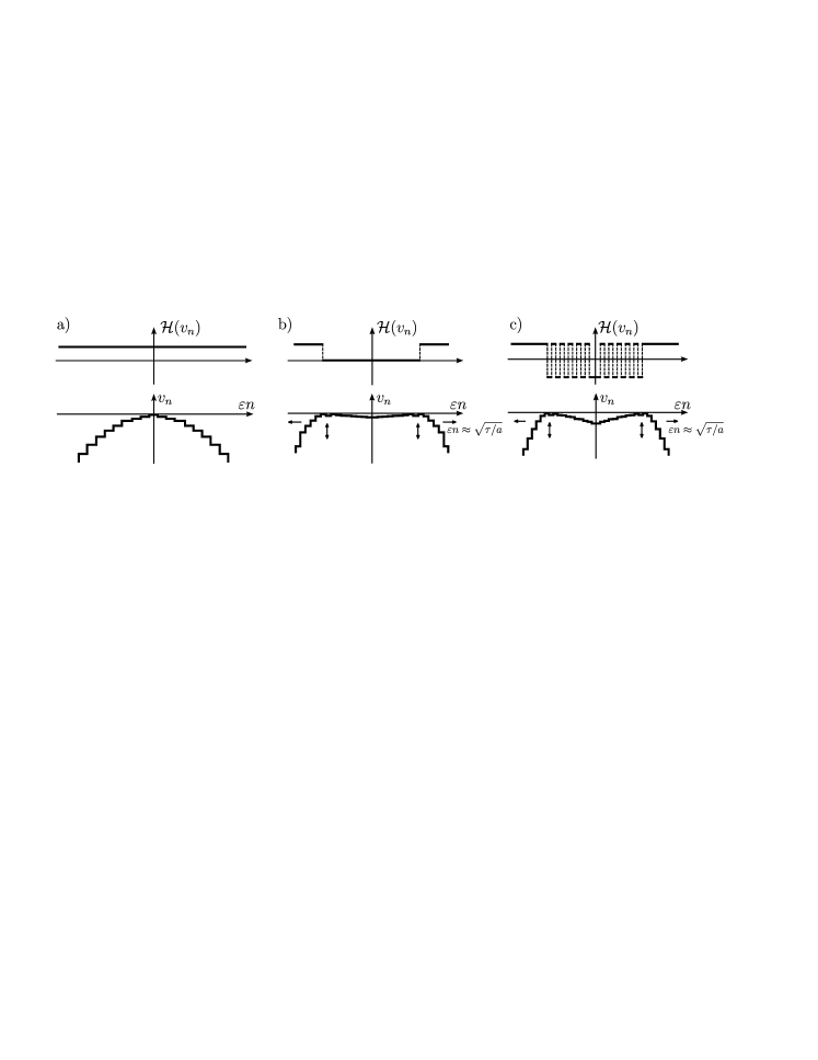
Figure 1.3: Upper graphs represent spatial profiles of the hysteresis ${\mathcal{H}}(v_{n})$ and lower graphs the spatial profiles of the solution $v_{n}$. a) Nontransverse initial data. b) Spatial profiles at a moment $\tau>0$ for $h_{2}=0$. c) Spatial profiles at a moment $\tau>0$ for $h_{2}=h_{1}>0$.

If $h_{2}=0$, then each node eventually achieves the threshold $\beta=0$ and thus ${\mathcal{H}}(v_{n})$ eventually switches from $h_{1}$ to $h_{2}=0$ for each $n\in{\mathbb{Z}}$. If $h_{2}>0$, then some nodes achieve the threshold and some do not. If we denote by $N_{1}(j)$ and $N_{2}(j)$ the number of nodes in the set $\{v_{0},v_{\pm 1},\dots,v_{\pm j}\}$ that switch and do not switch, respectively, on the time interval $[0,\infty)$, then numerics suggests that

$$\lim\limits_{j\to\infty}\dfrac{N_{2}(j)}{N_{1}(j)}=\dfrac{h_{2}}{h_{1}}.$$ (1.4)

Moreover, if $h_{2}/h_{1}=p_{2}/p_{1}$, where $p_{1}$ and $p_{2}$ are co-prime integers, then, for any $j$ large enough, the set $\{v_{j+1},\dots,v_{j+p_{1}+p_{2}}\}$ contains exactly $p_{1}$ nodes that switch and $p_{2}$ nodes that do not switch on the time interval $[0,\infty)$.

The next numerical observation is as follows. Let $\tau_{n}=\tau_{n}(\varepsilon)$ be the switching moment of the node $v_{n}(\tau;\varepsilon)$ if this node switches on the time interval $[0,\infty)$ and $\tau_{n}:=\infty$ otherwise. Then, for any fixed $h_{2}\geq 0$, the $\tau_{n}$’s that are finite satisfy, as $n\to\infty,$

$$\tau_{n}=a(\varepsilon n)^{2}+\begin{cases}\varepsilon^{2}O(\sqrt{n})&\text{if }h_{2}=0,\\ \varepsilon^{2}O(n)&\text{if }h_{2}>0,\end{cases}$$ (1.5)

where $a>0$ depends on $h_{1}/c$ but does not depend on $h_{2}$ or $\varepsilon$ and $O(\cdot)$ does not depend on $\varepsilon$.

Remark 1.1.

In Section 1.2, we will show that $\varepsilon$ in (1.3) can be scaled out, see scaling (1.8). In particular, all the numerical observations concerning the dynamics of $v_{n}$ have been done for $\varepsilon=1$ and then transferred to an arbitrary $\varepsilon$ according to the scaling in (1.8).

Consider the function

$$H(x,\tau;\varepsilon):={\mathcal{H}}(v_{n}(\cdot;\varepsilon))(\tau),\quad x\in[\varepsilon n-\varepsilon/2,\varepsilon n+\varepsilon/2),\ n\in{\mathbb{Z}},$$

which is supposed to approximate the hysteresis ${\mathcal{H}}(v(x,\cdot))(\tau)$ in (1.1). Assuming the dynamics (1.4) and (1.5) and taking into account Remark 1.1, we see that $H(x,\tau;\varepsilon)$ has no pointwise limit as $\varepsilon\to 0$, but converges in a certain weak sense to the function $H(x,\tau)$ given by $H(x,\tau)=0$ for $\tau>ax^{2}$ and $H(x,\tau)=h_{1}$ for $\tau<ax^{2}$. We emphasize that $H(x,\tau)$ does not depend on $h_{2}$ (because $a$ does not). On the other hand, if $h_{2}>0$, the hysteresis operator ${\mathcal{H}}(v(x,\cdot))(\tau)$ in (1.1) cannot take value $0$ by definition, which clarifies the essential difficulty with the well-posedness of the original problem (1.1) in the nontransverse case. To overcome the non-wellposedness, one need to allow the intermediate value $0$ for the hysteresis operator.

Such a re-definition of hysteresis is consistent with the behavior of $v(x,\tau)$ (also observed numerically) in the following sense. For a fixed $\varepsilon>0$, the spatial profile of $v_{n}(\cdot;\varepsilon)(\tau)$ forms two humps propagating away from the origin according to (1.5). The cavity between the humps has a bounded steepness characterized by the relations

$$|v_{k+1}(\tau;\varepsilon)-v_{k}(\tau;\varepsilon)|\leq b\varepsilon^{2},\quad|k|\leq n,\ \tau\geq\tau_{n},\ n=0,1,2,\dots,$$ (1.6)

where $b>0$ does not depend on $k$, $n$, and $\varepsilon$. As time goes on, the profile executes downwards and upwards motions, always remaining beneath the threshold $\beta=0$ and hitting this threshold at specific nodes characterized by (1.4). We call such a behavior of $v_{n}$ and ${\mathcal{H}}(v_{n})$ rattling. Furthermore, numerics indicates that, as $\varepsilon\to 0$, the function

$$V(x,\tau;\varepsilon):=v_{n}(\tau;\varepsilon),\quad x\in[\varepsilon n-\varepsilon/2,\varepsilon n+\varepsilon/2),\ n\in{\mathbb{Z}},$$

approximates a smooth function $V(x,\tau)$, which satisfies $V(x,\tau)=0$ for $\tau>ax^{2}$ due to (1.5) and (1.6). In other words, $V(x,\tau)$ sticks to the threshold line $\beta=0$ on the expanding interval $x\in(-\sqrt{\tau/a},\sqrt{\tau/a})$.

We recall paper [3], in which Alt proved the existence of a function $V(x,\tau)$ that satisfies the equation

$$V_{\tau}=V_{xx}+\gamma(x,\tau),$$

where $\gamma(x,\tau)={\mathcal{H}}(V(x,\cdot))(\tau)$ a.e. on the set $A:=\{(x,\tau):V(x,\tau)\neq\alpha,\beta\}$ and $\gamma(x,\tau)=0$ a.e. on the set $B:=\{(x,\tau):V(x,\tau)=\alpha\ \text{or}\ \beta\}$ (which potentially may have a nonzero measure). Thus, our heuristic argument provides a qualitative description of the sets $A$ and $B$ and justifies the completion of hysteresis by the zero value via the thermodynamical limit. To make this argument mathematically rigorous, we should first rigorously describe the rattling phenomenon in the discrete system (1.3). This is the central topic of the present paper, in which we concentrate on the case $h_{2}=0$ and develop general tools for treating discrete reaction-diffusion equations with discontinuous hysteresis. The application of these tools to the case $h_{2}>0$ will be a subject of a forthcoming paper. We expect that these tools will be applicable whenever $h_{2}/h_{1}$ is rational.

Before we proceed with the description of our tools and of the structure of the paper, let us make two more comments. First, the rattling phenomenon also occurs in multidimensional domains. For example, Fig. 1.4 illustrates the switching pattern for a two-dimensional analog of (1.3), where we have implemented spatial discretizations on the square and triangular lattices, respectively.

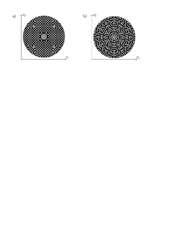
Figure 1.4: A snapshot for a time moment $\tau>0$ of a two-dimensional spatial profile of hysteresis taking values $h_{1}>4c>0$ and $h_{2}=h_{1}>0$. The nontrasverse initial data is given by $\varphi(x)=-c(x_{1}^{2}+x_{2}^{2})$. Grey (black) squares or hexagons correspond to the nodes that have (not) switched on the time interval $[0,\tau]$. a) Discretization on the square lattice. b) Discretization on the triangular lattice.

Moreover, numerical analysis of the Hoppensteadt–Jäger system indicates that the solution remains transverse as long as the central disc in Fig. 1.2 gets formed, but the formation of all the rings occurs via rattling.

Second, the rattling phenomenon is not a pure consequence of a discontinuous nature of hysteresis, but rather a consequence of bistability in a system. In particular, it persists in bistable slow-fast reaction-diffusion systems. The simplest example is the system

$$v_{\tau}=v_{xx}+w,\qquad\delta w_{\tau}=f(v,w),$$ (1.7)

where $\delta>0$ is a small parameter and the nullcline of $f(v,w)$ is $Z$- or $S$-shaped. Formally, system (1.7) can be treated as another regularization of system (1.1). In the case where the nullcline of $f(v,w)$ is $S$-shaped, one should replace $h_{1}$ and $-h_{2}$ in the definition of hysteresis ${\mathcal{H}}(v)$ by appropriate functions $H_{1}(v)$ and $H_{2}(v)$, see Fig. 1.5.

As $\delta\to 0$, the spatial profiles of $v$ and $w$ in (1.7) behave similarly to $V(x,\tau;\varepsilon)$ and $H(x,\tau;\varepsilon)$, respectively, as $\varepsilon\to 0$, see Fig. 1.6, with the exception that the profile of $w$ remains continuous and forms steep transition layers between mildly sloping steps of width tending to $0$ as $\delta\to 0$. Interestingly, the time-scale separation parameter $\delta$ in (1.7) yields the same effect as the grid-size parameter $\varepsilon$ in (1.3). As far as we know, such a rattling phenomenon for slow-fast systems has not been explained in the literature, either.

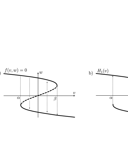
Figure 1.5: a) The nullcline of the $S$-shaped nonlinearity $f(v,w)$. b) Hysteresis with nonconstant branches $H_{1}(v)$ and $H_{2}(v)$.

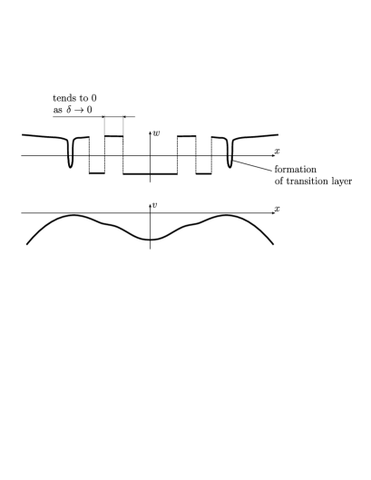
Figure 1.6: Upper and lower graphs are spatial profiles of the solution $w(x,\tau)$ and $v(x,\tau)$, respectively, for problem (1.7) with initial data $v|_{\tau=0}=-cx^{2}+o(x^{2})$, $w|_{\tau=0}=h_{1}$.

1.2 Structure of the paper

Now we come back to the main topic of this paper, namely, discrete system (1.3). As it was mentioned in Remark 1.1, $\varepsilon$ in (1.3) can be scaled out. Indeed, setting

$$t:=\varepsilon^{-2}\tau,\quad u_{n}(t):=\varepsilon^{-2}v_{n}(\tau;\varepsilon)$$ (1.8)

and using the equalities (recall that $\alpha=-\infty$ and $\beta=0$)

$${\mathcal{H}}(v_{n})(\tau)={\mathcal{H}}(\varepsilon^{2}u_{n}(\varepsilon^{-2}\cdot))(\tau)={\mathcal{H}}(u_{n}(\varepsilon^{-2}\cdot))(\tau)={\mathcal{H}}(u_{n})(\varepsilon^{-2}\tau)={\mathcal{H}}(u_{n})(t),$$

we can rewrite (1.3) as follows:

$$\left\{\begin{aligned} &\dot{u}_{n}=\Delta u_{n}+{\mathcal{H}}(u_{n}),\quad t>0,\ n\in{\mathbb{Z}},\\ &u_{n}(0)=-cn^{2},\quad n\in{\mathbb{Z}},\end{aligned}\right.$$ (1.9)

where $\dot{}=d/dt$. Problem (1.9) does not involve $\varepsilon$, which justifies the fact that $u_{n}(t)$ in (1.8) does not depend on $\varepsilon$. Note that $c$ in (1.9) could be also scaled out replacing $u_{n}(t)$, $h_{1}$ and $-h_{2}$ by $c\tilde{u}_{n}(t)$, $c\tilde{h}_{1}$ and $-c\tilde{h}_{2}$, respectively. We prefer not to do this, in order to keep track of what exactly is influenced in our intermediate calculations by the “tangency” constant $c$.

From now on, we concentrate on the case $h_{2}=0$. Due to (1.5) and (1.8), the asymptotics for the switching moment $t_{n}$ of the node $u_{n}(t)$ is expected to be

$$t_{n}=an^{2}+q_{n},\quad|q_{n}|\leq E\sqrt{n},$$ (1.10)

where $E>0$ does not depend on $n\in{\mathbb{Z}}$.

Our main result (Theorem 3.2) is as follows. Let $h_{1}>2c>0$ and $h_{2}=0$. Assume that

$$\text{finitely many nodes}\ u_{n}(t)$$ (1.11)

$$\text{switch at moments}\ t_{n},\ n=0,1,\dots,n_{0},\ \text{satisfying\leavevmode\nobreak\ \eqref{eqtnExpected}},$$

where the constants $a=a(h_{1}/c)>0$ and $n_{0}=n_{0}(E)=n_{0}(E,h_{1},c)$ will be explicitly specified in the main text. Then each node $u_{n}(t)$, $n\in{\mathbb{Z}}$, switches; moreover, the switching occurs at a time moment $t_{n}$ satisfying (1.10).

Since we will provide an explicit formula for the solution $u_{n}(t)$, the fulfillment of finitely many assumptions (1.11) can be verified numerically with an arbitrary accuracy for any given values of $h_{1}$ and $c$ (see Fig. 1.7).

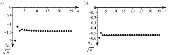
Figure 1.7: Values of $q_{n}/\sqrt{n}$ for $c=1/2$ and a) $h_{1}=1.5$, b) $h_{1}=2.0$.

The paper is organized as follows. In Section 2, we give definitions for the hysteresis operator and for the solution of problem (1.9). Next, we formulate the existence and uniqueness theorem (Theorem 2.5), which includes a representation of the solution $u_{n}(t)$ via the discrete Green function $y_{n}(t)$. In particular, Theorem 2.5 implies that $u_{n}(t)=u_{-n}(t)$, $n\in{\mathbb{Z}}$.

In Section 3, we formulate our main result (Theorem 3.2).

In Section 4, we formulate three main ingredients for the proof of the main result.

1. The first ingredient is asymptotic formulas for the Green function $y_{n}(t)$ and for its time derivatives, which were derived in [11].

2. The second ingredient is three equations for finding the constant $a$ from equation (1.10). The equivalence of these equations as well as the existence and uniqueness of their root $a>0$ are proved in Appendix A.

3. The third ingredient is the approximation of some singular integrals by Riemann sums and corresponding error estimates, which are proved in [15].

Sections 5, 6, and 7 are three key steps in the proof of our main result. The scheme of the proof is inductive. Assume we have proved that $t_{0},t_{1},\dots,t_{n-1}$ satisfy (1.10) for some fixed $n\geq n_{0}+1$. We fix the hysteresis configuration, i.e., set $H_{n}:={\mathcal{H}}(u_{n})(t_{n-1})$ and consider the solution $v_{n}(t)$ of the problem

$$\left\{\begin{aligned} &\dot{v}_{n}=\Delta v_{n}+H_{n},\quad t>t_{n-1},\ n\in{\mathbb{Z}},\\ &v_{n}(t_{n-1})=u(t_{n-1}),\quad n\in{\mathbb{Z}}\end{aligned}\right.$$

(we abuse the notation by using the same letter $v$ as in Section 1.1). Obviously, $v_{n}(t)=u_{n}(t)$ as long as the nodes $v_{n}(t),v_{n+1}(t),v_{n+2}(t),\dots$ remain below the threshold $\beta=0$.

The main theorem of Section 5 (Theorem 5.4) claims that the equation $v_{n}(an^{2}+q_{n})=0$ has a root $q_{n}$ satisfying (1.10). To prove this, we use an explicit representation of $v_{n}(t)$ via the convolution of $H_{n}$ with the Green function $y_{n}(t)$ (see (5.19)). Then we use asymptotic formulas for $y_{n}(t)$ (the first ingredient from Section 4) and replace the convolution by a singular integral (the third ingredient from Section 4). As a result, we obtain a leading order term of order $n^{2}$, which depends only on $a$ and $h_{1}/c$, and a remainder of order $\sqrt{n}$, which also depends on $q_{0},q_{1},\dots,q_{n-1}$ (that are known due to the inductive hypothesis) and on the unknown $q_{n}$. It appears that the coefficient at $n^{2}$ vanishes due to the choice of $a$ (the second ingredient from Section 4). The hard part is to show that the remainder vanishes for some $q_{n}$ satisfying (1.10). This is done by an application of Brouwer’s fixed-point theorem.

The time moment $t_{n}:=an^{2}+q_{n}$ given by Theorem 5.4 is a candidate for being the switching moment of $u_{n}(t)$. To show that it is the switching moment, we have to prove that neither of the nodes $v_{n+1}(t),v_{n+2}(t),\dots$ achieves the value $\beta=0$ on the interval $(t_{n-1},t_{n}]$, while $v_{n}(t)$ achieves it at the moment $t_{n}$ for the first time. This is done in Sections 6 and 7.

In Section 6, we prove that $v_{n+1}(t_{n})<0$ (Theorem 6.2). To do so, we estimate the gradient $\nabla v_{n}(t_{n}):=v_{n+1}(t_{n})-v_{n}(t_{n})$ by using the representation of $\nabla v_{n}(t)$ via the gradient $\nabla y_{n}(t)$ of the Green function, applying asymptotic formulas for $\nabla y_{n}(t)$ (recall the first ingredient from Section 4) and again replacing the corresponding convolution by an integral (recall the third ingredient from Section 4). It appears that the leading order term of order $n$ vanishes due to the second ingredient from Section 4. Thus, we calculate the next term in the asymptotics, which turns out to be $-3h_{1}/4<0$. Hence, $v_{n+1}(t_{n})=\nabla v_{n}(t_{n})\leq-3h_{1}/8<0$.

In Section 7, we first show that $v_{n}(t)$ does not achieve the threshold $\beta=0$ for $t\in(t_{n-1},t_{n})$ (Theorem 7.1). To do so, we divide the interval $(t_{n-1},t_{n})$ into two parts. We prove that the function $\dot{v}_{n}(t)$ is so small on the first interval that it cannot overcome the distance exceeding $-3h_{1}/8$ (the value coming from Theorem 6.2 with $n+1$ replaced by $n$). Then we prove that $\ddot{v}_{n}(t)$ is nonnegative on the second interval. Hence, the equation $v_{n}(t)=0$ has a unique root, which must be $t_{n}$. In particular, $v_{n}(t)<0$ for $t\in(t_{n-1},t_{n})$. Finally, we show that $\nabla v_{j}(t)<0$ for all $t\in(t_{n-1},t_{n}]$ and $j\geq n$, which implies that the nodes $v_{n+1}(t),v_{n+2}(t),\dots$ remain negative for $t\in(t_{n-1},t_{n}]$ (Theorem 7.3).

In Section 8, we combine the results from Sections 5, 6, and 7 and rigorously implement the inductive scheme, which completes the proof of the main result, namely, Theorem 3.2.

The crucial role in our main result (Theorem 3.2) is played by the number $n_{0}=n_{0}(E)$, which determines the number of switchings one has to check “by hand” (see (1.11)). The number $n_{0}(E)$ is determined explicitly by 12 inequalities that must hold for $n\geq n_{0}(E)$. Each inequality is referred to as a requirement and is introduced in the text where it is used for the first time. These 12 requirements contain constants that are also introduced in the text where they are used for the first time. For reader’s convenience, we have collected all those constants in Appendices B.1–B.3 and the 12 requirements in Appendix B.4.

The graphs in Fig. 1.8 represent the values of $a$, $E$, and $n_{0}(E)$ that fulfill assumptions (1.11) for $c=1/2$ and $h_{1}=1.1,1.2,1.3,\dots,2.5$.

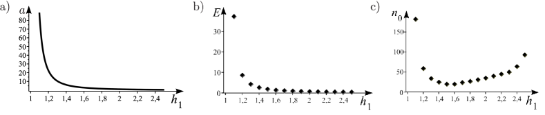
Figure 1.8: Dependence on $h_{1}$ of the values of $a$, $E$, and $n_{0}(E)$ that fulfill assumptions (1.11) for $c=1/2$. a) The values of $a$ are found explicitly for all $h_{1}>1$ (see Section 4.2 below). b), c) The values of $E$ and $n_{0}(E)$ are calculated numerically for $h_{1}=1.1,1.2,1.3,\dots,2.5$.

2 Setting of the problem and a proof of its well-posedness

For a sequence $\{v_{n}\}_{n\in{\mathbb{Z}}}$ of real numbers, we use the notation

$$\nabla v_{n}:=v_{n+1}-v_{n},\qquad\Delta v_{n}:=\nabla v_{n}-\nabla v_{n-1}=v_{n-1}-2v_{n}+v_{n+1}.$$

Let $\{u_{n}(t)\}_{n\in{\mathbb{Z}}}$ be real-valued functions defined for $t\geq 0$. We study the problem

$$\dot{u}_{n}=\Delta u_{n}+{\mathcal{H}}(u_{n}),\quad t>0,\ n\in{\mathbb{Z}},$$ (2.1)

$$u_{n}(0)=-cn^{2},\quad n\in\mathbb{Z},$$ (2.2)

where $c>0$ and ${\mathcal{H}}(w)(t)$, $t\geq 0$, is the hysteresis operator defined for functions $w\in C[0,\infty)$ such that $w(0)\leq 0$ by

$${\mathcal{H}}(w)(t):=\begin{cases}h_{1}&\text{if }w(s)<0\ \text{for all }s\in[0,t],\\ 0&\text{if }w(s)=0\ \text{for some}\ s\in[0,t],\end{cases}$$ (2.3)

where $h_{1}>0$ is fixed. In other words, the output of hysteresis is $h_{1}$ unless the input achieves the zero threshold; at this moment, the hysteresis switches and since then the output of hysteresis remains $0$. In the context of problem (2.1)–(2.3), we will say “a node $u_{n}(t)$ switches” or “a node $n$ switches” whenever $u_{n}(t)$ achieves the value zero for the first time.

Remark 2.1.

In the terminology of, e.g., [20, 27], the hysteresis operator (2.3) is a non-ideal relay with the thresholds $-\infty$ and $0$; see Fig. 1.1.b.

From now on, we assume throughout that the following condition holds.

Condition 2.2.

$h_{1}>2c>0$.

We note that the function ${\mathcal{H}}(v)(t)$ may have discontinuity (actually, at most one) even if $v\in C^{\infty}[0,\infty)$. Therefore, one cannot expect that a solution of problem (2.1)–(2.3) is continuously differentiable on $[0,\infty)$. Thus, we define a solution as follows.

Definition 2.3.

We say that a sequence $\{u_{n}(t)\}_{n\in{\mathbb{Z}}}$ is a solution of problem (2.1)–(2.3) on the time interval $(0,T)$, $T>0$, if

1. $u_{n}\in C[0,T]$ for all $n\in{\mathbb{Z}}$,

2. for each $t\in[0,T]$, there exists $A,\alpha\geq 0$ such that $\sup\limits_{s\in[0,t]}|u_{n}(s)|\leq Ae^{\alpha|n|}$ for all $n\in{\mathbb{Z}}$,

3. there is a finite sequence $0=\tau_{0}<\tau_{1}<\dots<\tau_{J}=T$, $J\geq 1$, such that $u_{n}\in C^{1}(\tau_{j},\tau_{j+1})$ for all $n\in{\mathbb{Z}}$ and $j=0,\dots,J-1$,

4. the equations in (2.1) hold in $(\tau_{j},\tau_{j+1})$ for all $n\in{\mathbb{Z}}$ and $j=0,\dots,J-1$,

5. $u_{n}(0)=-cn^{2}$ for all $n\in{\mathbb{Z}}$.

We say that a sequence $\{u_{n}(t)\}_{n\in{\mathbb{Z}}}$ is a solution of problem (2.1)–(2.3) on the time interval $(0,\infty)$ if it is a solution on $(0,T)$ for all $T>0$.

Remark 2.4.

If $\{u_{n}(t)\}_{n\in{\mathbb{Z}}}$ is a solution, then, as we have mentioned above, the function ${\mathcal{H}}(u_{n})(t)$ has at most one discontinuity point for each fixed $n\in{\mathbb{Z}}$. Hence, the equations in (2.1) imply that each function $\dot{u}_{n}(t)$ has at most one discontinuity point on $[0,\infty)$.

Before we treat existence and uniqueness of a solution, let us introduce one of our main tools, namely, the so-called discrete Green function

$$y_{n}(t):=\dfrac{1}{2\pi}\int_{-\pi}^{\pi}\dfrac{1-e^{-2t(1-\cos\theta)}}{2(1-\cos\theta)}\,e^{in\theta}\,d\theta,\quad t\geq 0.$$ (2.4)

One can directly check that $y_{n}\in C^{\infty}[0,\infty)$ and $y_{n}(t)$ solves the problem

$$\left\{\begin{aligned} &\dot{y}_{0}=\Delta y_{0}+1,&&t>0,\\ &\dot{y}_{n}=\Delta y_{n},&&t>0,\ n\neq 0,\\ &y_{n}(0)=0,&&n\in\mathbb{Z}.\end{aligned}\right.$$ (2.5)

Below, we will use the fact that

$$\dot{y}_{n+1}(t)<\dot{y}_{n}(t),\quad t>0,\ n=0,1,2,\dots,$$ (2.6)

which follows from the formula $\dot{y}_{n}(t)=e^{-2t}I_{n}(2t)$, where $I_{n}(s)$ is the modified Bessel function of the first kind (see [1, Sec. 9.6.19]), and from, e.g., [4]. We will also use the estimate, which follows from the series representation of the modified Bessel function [1, Sec. 9.6.10]:

$$0\leq\dot{y}_{n}(t)=e^{-2t}I_{n}(2t)=e^{-2t}t^{|n|}\sum\limits_{m=0}^{\infty}\dfrac{t^{2m}}{m!(m+|n|)!}\leq\dfrac{e^{t^{2}-2t}t^{|n|}}{|n|!},\quad n\in{\mathbb{Z}}.$$ (2.7)

Below we prove the following existence and uniqueness result.

Theorem 2.5.

1. Problem (2.1)–(2.3) has a unique solution $\{u_{n}(t)\}_{n\in{\mathbb{Z}}}$ on the time interval $(0,\infty)$.

2. Let $t_{n}$ be the switching moment of the node $u_{n}(t)$ if this node switches on the time interval $[0,\infty)$ and $t_{n}:=\infty$ otherwise. Then

   $$t_{n}\geq\dfrac{cn^{2}}{h_{1}-2c},\quad n\in{\mathbb{Z}}.$$ (2.8)

3. Let $S(t)$ be the set of nodes that switch on the time interval $[0,t]$, i.e.,

   $$S(t):=\{k\in{\mathbb{Z}}:{\mathcal{H}}(u_{k})(t)=0\},$$ (2.9)

   and let $|S(t)|$ be the number of elements in $S(t)$. Then $S(t)$ is finite for each $t>0$, symmetric with respect to the origin, $|S(t)|\to\infty$ as $t\to\infty$, and

   $$u_{n}(t)=-cn^{2}+(h_{1}-2c)t-h_{1}\sum\limits_{k\in S(t)}y_{n-k}(t-t_{k}),\quad t\in[0,\infty),$$ (2.10)

   where we put $y_{n-k}(t-t_{k})=0$ for $t<t_{k}$,

4. for each $n\in{\mathbb{N}}$, we have $t_{-n}=t_{n}$ and $u_{-n}(t)\equiv u_{n}(t)$.

Proof.

Step 1. Using (2.5), we see that the functions

$$z_{n}^{(1)}(t):=-cn^{2}+(h_{1}-2c)t-h_{1}y_{n}(t),\quad n\in{\mathbb{Z}},$$ (2.11)

satisfy the initial condition (2.2) and the equation in (2.1) as long as $z_{n}^{(1)}(t)<0$ for all $n\in{\mathbb{Z}}\setminus\{0\}$. By comparing $z_{n}^{(1)}(t)$ with the solution

$$z_{n}^{+}(t)=-cn^{2}+(h_{1}-2c)t$$ (2.12)

of problem (2.1)–(2.3) with ${\mathcal{H}}(u_{n})$ replaced by $h_{1}$ for all $n\in{\mathbb{Z}}$, it is not difficult to see that

$$z_{n}^{(1)}(t)\leq z_{n}^{+}(t),\quad t\geq 0,\ n\in{\mathbb{Z}}.$$ (2.13)

Therefore, the time moment $t_{n}$ at which $z_{n}(t)$ vanishes for the first time is not less than the moment $t_{n}^{+}=cn^{2}/(h_{1}-2c)$ at which $z_{n}^{+}(t)$ vanishes.

In particular, $z_{n}^{(1)}(t)<0$ for all $n\in{\mathbb{Z}}\setminus\{0\}$ and $t\in[0,c/(h_{1}-2c))$. Let $\tau_{1}:=\sup\{t>0:z_{n}^{(1)}(t)<0\ \forall n\in{\mathbb{Z}}\setminus\{0\}\}$. It follows from (2.11), (4.3), and (4.7) that $\tau_{1}$ is finite. As we have seen, $\tau_{1}\geq c/(h_{1}-2c)>0$. Furthermore, $z_{n}^{(1)}(t)$ satisfy the growth condition from item 2 of Definition 2.3 for $t\in[0,\tau_{1}]$. This follows from (2.11) and the fact that $|y_{n}(t)|$ given by (2.4) are bounded on any finite time interval, uniformly with respect to $n\in{\mathbb{Z}}$. Thus, $u_{n}(t):=z_{n}^{(1)}(t)$ is a solution of problem (2.1)–(2.3) on the time interval $(0,\tau_{1})$.

Let us prove that the solution $u_{n}(t)$ is unique on $(0,\tau_{1})$. Assume we have another solution $\tilde{u}_{n}(t)$ on a time interval $(0,\tilde{\tau}_{1})$, where $\tilde{\tau}_{1}\leq\tau_{1}$ is such that $\tilde{u}_{n}(t)<0$ for all $t\in(0,\tau_{1})$ and $n\in{\mathbb{Z}}\setminus\{0\}$. Then the difference $w_{n}(t):=u_{n}(t)-\tilde{u}_{n}(t)$ must satisfy the homogeneous diffusion equation on the time interval $(0,\tilde{\tau}_{1})$ with the zero initial data

$$\dot{w}_{n}(t) =\Delta w_{n}(t),\quad t\in(0,\tilde{\tau}_{1}),\ n\in{\mathbb{Z}},$$

$$w_{n}(0) =0,\quad n\in{\mathbb{Z}}.$$

If we looked for solutions that are square summable with respect to $n\in{\mathbb{Z}}$, then the application of the discrete Fourier transform would immediately imply that all $w_{n}(t)\equiv 0$. However, we are interested in solutions that may have exponential growth with respect to $n\in{\mathbb{N}}$ (see item 2 in Definition 2.3). We will argue as follows. For each $N\in{\mathbb{N}}$, we consider the functions

$$\zeta_{n}(t)=\zeta_{n}^{N}(t):=w_{n}(t)\ \text{for }|n|\leq N,\qquad\zeta_{n}(t)=\zeta_{n}^{N}(t):=0\ \text{for }|n|\geq N+1.$$ (2.14)

They satisfy the relations

$$\dot{\zeta}_{n}(t) =\Delta\zeta_{n}(t)+G_{n}^{N}(t),\quad t\in(0,\tilde{\tau}_{1}),\ n\in{\mathbb{Z}},$$ (2.15)

$$\zeta_{n}(0) =0,\quad n\in{\mathbb{Z}},$$

where $G_{n}^{N}(t)=0$ for $|n|\leq N-1$ and $|n|\geq N+2$, $G_{\pm N}^{N}(t)=w_{\pm(N+1)}(t)$, and $G_{\pm(N+1)}^{N}(t)=-w_{\pm N}(t)$. Since no more than finitely many elements in the sequences $\{\zeta_{n}(t)\}_{n\in{\mathbb{Z}}}$ and $\{G_{n}^{N}(t)\}_{n\in{\mathbb{Z}}}$ are nonzero, we can apply the discrete Fourier transform to (2.15) and obtain

$$\zeta_{n}^{N}(t)=\sum\limits_{|k|=N}^{N+1}\int_{0}^{t}\dot{y}_{n-k}(t-s)\,G_{k}^{N}(s)\,ds,\quad t\in[0,\tilde{\tau}_{1}],\ n\in{\mathbb{Z}}.$$ (2.16)

Now let us fix $n\geq 0$ and $t\in[0,\tilde{\tau}_{1}]$. By assumption, there exist $A,\alpha\geq 0$ such that

$$\sup\limits_{s\in[0,t]}|w_{k}(s)|\leq Ae^{\alpha|k|},\quad k\in{\mathbb{Z}}.$$ (2.17)

Combining (2.14), (2.16), (2.7), (2.17) and choosing $N\geq n$, we have

$$|w_{n}(t)|=|\zeta_{n}^{N}(t)|\leq t\sum\limits_{|k|=N}^{N+1}\sup\limits_{s\in[0,t]}\left(|\dot{y}_{n-k}(s)|\cdot|G_{k}^{N}(s)|\right)\leq c\dfrac{t^{N}e^{\alpha N}}{(N-n)!}\to 0\quad\text{as }N\to\infty,$$

where $c=c(n,t)\geq 0$ does not depend on $N$. Therefore, $w_{-n}(t)\equiv w_{n}(t)\equiv 0$. This proves that $u_{n}(t)$ is a unique solution of problem (2.1)–(2.3) on the time interval $(0,\tau_{1})$.

Step 2. Set $S(\tau_{1}):=\{0\}\cup\{n\in{\mathbb{Z}}:z_{n}^{(1)}(\tau_{1})=0$}, cf. (2.9). Due to (2.12) and (2.13), the set $S(\tau_{1})$ is finite. Due to (2.11) and the symmetry $y_{n}(t)\equiv y_{-n}(t)$, the set $S(\tau_{1})$ is symmetric with respect to the origin. Note that $t_{0}=0$ is the switching moment of the node $0$, while $t_{n}=\tau_{1}$ are the switching moments of the nodes $n\in S(\tau_{1})\setminus\{0\}$.

Using (2.5) and assuming $y_{n}(t):=0$ for $t<0$, we see that the functions

$$z_{n}^{(2)}(t) =-cn^{2}+(h_{1}-2c)t-h_{1}\left(y_{n}(t)+\sum\limits_{k\in S(\tau_{1})\setminus\{0\}}y_{n-k}(t-\tau_{1})\right)$$ (2.18)

$$=-cn^{2}+(h_{1}-2c)t-h_{1}\sum\limits_{k\in S(\tau_{1})}y_{n-k}(t-t_{k}),\quad t\in[0,\infty),$$

satisfy the equations in (2.1) as long as $z_{n}^{(2)}(t)<0$ for all $n\in{\mathbb{Z}}\setminus S(\tau_{1})$, i.e., as long as $S(t)=S(\tau_{1})$. Obviously, $z_{n}^{(2)}(t)$ also satisfy the initial condition (2.2).

As in Step 1, we see that the time moment $t_{n}$ at which $z_{n}(t)$, $n\in{\mathbb{Z}}\setminus S(\tau_{1})$, vanishes for the first time is not less than $cn^{2}/(h_{1}-2c)$. Hence, there is a positive time interval (of length bigger than $\tau_{1}$) on which $z_{n}^{(2)}(t)<0$ for all $n\in{\mathbb{Z}}\setminus S(\tau_{1})$.

Let $\tau_{2}:=\sup\{t>0:z_{n}^{(2)}(t)<0\ \forall n\in{\mathbb{Z}}\setminus S(\tau_{1})\}$. It follows from (2.11), (4.3), and (4.7) that $\tau_{2}$ is finite. We have proved that $\tau_{2}>\tau_{1}$. Furthermore, $z_{n}^{(2)}(t)$ satisfy the growth condition from item 2 of Definition 2.3 for $t\in[0,\tau_{2}]$. Thus, $u_{n}(t):=z_{n}^{(2)}(t)$ is a solution of problem (2.1)–(2.3) on the time interval $(0,\tau_{2})$. Note that $u_{n}(t)=z_{n}^{(1)}(t)$ for $t\in[0,\tau_{1}]$. The uniqueness of $u_{n}(t)$ on the interval $(\tau_{1},\tau_{2})$ can be proved similarly to Step 1.

Continuing these steps, we obtain the desired infinite sequence $\{\tau_{j}\}_{j\geq 0}$ from Definition 2.3. On each step, we compare $u_{n}(t)$ with $z_{n}^{+}(t)$ given by (2.12) and conclude that the switching moments satisfy $t_{n}\geq cn^{2}/(h_{1}-2c)$. Hence, $\tau_{j}\to\infty$ as $j\to\infty$. ∎

3 Main result

We recall that Condition 2.2 is assumed to hold throughout. Below in the text we define $a>0$ (see Lemma 4.2), $E_{0}>0$ (see (5.12)) and an increasing function $n_{0}:(E_{0},\infty)\to{\mathbb{N}}$ (see Requirements 1–12 in Section B.4).

Definition 3.1.

We say that a number $E\geq E_{0}$ is admissible if the following holds:

1. each node $u_{k}$, $k=0,\pm 1\,\dots,\pm n_{0}=\pm n_{0}(E)$ switches at a moment $t_{k}$ satisfying

   $$t_{k}=ak^{2}+q_{k},\quad|q_{k}|\leq E\sqrt{n_{0}},$$ (3.1)

   while neither of the nodes $u_{\pm(n_{0}+1)},u_{\pm(n_{0}+2)},\dots$ switches on the time interval $[0,t_{n_{0}}]$;

2. at the switching moment $t_{n_{0}}$, we have

   $$u_{n_{0}+1}(t_{n_{0}})=\nabla u_{n_{0}}(t_{n_{0}})\leq-\dfrac{3h_{1}}{8}.$$ (3.2)

The main result of this paper is as follows. If finitely many nodes $k=0,\dots,n_{0}(E)$ switch at time moments $t_{k}$ satisfying (3.1), then all the nodes $n\in\mathbb{Z}$ will switch and their switching moments will be of order $an^{2}$. On Fig. 1.8.b, one can see the values of admissible $E$, which we found numerically for $c=1/2$ and $h_{1}=1.1,1.2,1.3,\dots,2.5$. Figures 1.8.a and 1.8.c depict corresponding values of $a$ and $n_{0}(E)$, respectively.

The rigourous formulation of our main result is as follows.

Theorem 3.2.

Assume that $E\geq E_{0}$ is an admissible number, and let $n_{0}=n_{0}(E)$. Then for all $n\geq n_{0}+1$$:$

1. Each of the nodes $u_{n}$ switches at a moment $t_{n}$ satisfying

   $$t_{n}=an^{2}+q_{n},\quad|q_{n}|\leq E\sqrt{n},$$ (3.3)

   $$t_{k}<t_{n_{0}}<t_{n_{0}+1}<\dots,\quad k=0,1,\dots,n_{0}-1,$$

2. There exists $A_{\nabla}>0$ depending on $h_{1},c,E$, but not on $n$, such that

   $$\left|\nabla u_{n}(t_{n})+\dfrac{3h_{1}}{4}\right|\leq A_{\nabla}n^{-1/2},\qquad\nabla u_{n}(t_{n})\leq-\dfrac{3h_{1}}{8}.$$

4 Auxiliary Statements

In this section, we formulate several auxiliary statements. Each of them is a key ingredient in the proof of our main result, i.e., Theorem 3.2.

In Section 4.1 (Proposition 4.1), we establish asymptotic formulas for the discrete Green function $y_{n}(t)$ given by (2.4). It is essential that the leading order terms in the asymptotics depend only on $n/\sqrt{t}$, while the remainders are estimated uniformly with respect to $n$.

In Section 4.2, we consider three expressions containing integrals (4.12) of leading order terms in the asymptotics of $y_{n}(t)$, $\nabla y_{n}(t)$, and $\dot{y}_{n}(t)$, respectively. These three expressions will enter the leading order terms in asymptotic formulas for $u_{n}(t_{n})$, $\nabla u_{n}(t_{n})$, and $\dot{u}_{n}(t_{n})$. In Proposition 4.2, we show that these terms vanish for the same value of $a$, thus determining the “propagation rate” $an^{2}$ in the switching moment asymptotics for $t_{n}$ in (3.1) and (3.3).

In Section 4.3, we elaborate on properties of integrals (4.12) from Section 4.2. In the proof of our main result, these integrals will play the role of approximation of some Riemann sums. Note that the corresponding integrands are not smooth functions, but have singularities of order $(1-x)^{1/2}$ or $(1-x)^{-1/2}$ at $x=1$. In Propositions 4.3 and 4.4, we provide error estimates for approximation of such integrals by their Riemann sums.

4.1 Properties of the discrete Green function $y_{n}(t)$

Consider the functions $h,f,g,\tilde{f}:{\mathbb{R}}^{+}\to{\mathbb{R}}$ given by

$$h(x):=\dfrac{1}{2\sqrt{\pi}}\,e^{-\frac{x^{2}}{4}},\quad f(x):=2x\int\limits_{x}^{\infty}y^{-2}h(y)\,dy,\quad g(x):=f^{\prime}(x),\quad\tilde{f}(x):=-\frac{h^{\prime\prime\prime}(x)}{6x}.$$ (4.1)

Note that these functions belong to $C^{\infty}[0,\infty)$ and decay to zero as $x\to\infty$, together with all their derivatives, faster than any exponential. Moreover,

$$h(x)=g^{\prime}(x)=f^{\prime\prime}(x),\quad 2h(x)+xg(x)-f(x)=0,\quad g(0)=-\frac{1}{2}.$$ (4.2)

Consider the functions $r_{0},\tilde{r}_{1},r_{1},r_{2},w_{0},w_{1}:({\mathbb{N}}\cup\{0\})\times{\mathbb{R}}_{+}\to{\mathbb{R}}$ satisfying the following relations for $n=0,1,2,\dots$ and $t>0$:

$$y_{n}(t) =\sqrt{t}f\!\left(\!\dfrac{n}{\sqrt{t}}\!\right)+r_{0}(n,t), y_{n}(t) =\sqrt{t}f\!\left(\!\dfrac{n}{\sqrt{t}}\!\right)+\frac{1}{\sqrt{t}}\tilde{f}\!\left(\!\dfrac{n}{\sqrt{t}}\!\right)+\tilde{r}_{1}(n,t),$$ (4.3)

$$\dot{y}_{n}(t) =\frac{1}{\sqrt{t}}h\!\left(\!\dfrac{n}{\sqrt{t}}\!\right)+r_{1}(n,t), \ddot{y}_{n}(t) =\frac{1}{t\sqrt{t}}h^{\prime\prime}\!\left(\!\dfrac{n}{\sqrt{t}}\!\right)+r_{2}(n,t),$$ (4.4)

$$\nabla\dot{y}_{n}(t) =\frac{1}{t}h^{\prime}\!\left(\!\dfrac{n}{\sqrt{t}}\!\right)+w_{1}(n,t), \nabla y_{n}(t) =g\!\left(\!\dfrac{n}{\sqrt{t}}\!\right)+\frac{1}{2\sqrt{t}}h\!\left(\!\dfrac{n}{\sqrt{t}}\!\right)+w_{0}(n,t).$$ (4.5)

We fix throughout the paper

$$\tau_{0}>0.$$ (4.6)

The following estimates are proved in [11].

Proposition 4.1.

There exist constants $A_{0},A_{1},A_{2},\tilde{A}_{1},B_{0},B_{1},A_{2}^{*},B_{2}^{*}>0$ $($depending on $\tau_{0}$$)$ such that, for all $t\geq\tau_{0}$, $n=0,1,2,\dots,$ and $i=0,1,2$, the following inequalities hold$:$

$$|r_{i}(n,t)| \leq A_{i}\frac{1}{t^{i}\sqrt{t}}, |\tilde{r}_{1}(n,t)| \leq\tilde{A}_{1}\frac{1}{t\sqrt{t}},$$ (4.7)

$$|w_{0}(n,t)| \leq B_{0}\frac{1}{t}, |w_{1}(n,t)| \leq B_{1}\frac{1}{t\sqrt{t}},$$ (4.8)

$$|\ddot{y}_{n}(t)| \leq A_{2}^{*}\frac{1}{t\sqrt{t}}, |\nabla\ddot{y}_{n}(t)| \leq B_{2}^{*}\frac{1}{t^{2}}.$$ (4.9)

4.2 Equivalence of some equations

Consider the functions

$$F(a,x) :=\sqrt{a(1-x^{2})}\,f\left(\dfrac{1}{\sqrt{a}}\sqrt{\dfrac{1-x}{1+x}}\right), G(a,x) :=g\left(\dfrac{1}{\sqrt{a}}\sqrt{\dfrac{1-x}{1+x}}\right),$$ (4.10)

$$H(a,x) :=\dfrac{1}{\sqrt{a(1-x^{2})}}\,h\left(\dfrac{1}{\sqrt{a}}\sqrt{\dfrac{1-x}{1+x}}\right), H_{1}(a,x) :=\dfrac{1}{a(1-x^{2})}\!h^{\prime}\!\left(\dfrac{1}{\sqrt{a}}\sqrt{\dfrac{1-x}{1+x}}\right),$$ (4.11)

where $a>0$, $x\in(-1,1)$ and $f,g,h$ are given by (4.1). Set

$$I_{F}(a):=\int_{-1}^{1}F(a,x)dx,\quad I_{G}(a):=\int_{-1}^{1}G(a,x)dx,\quad I_{H}(a):=\int_{-1}^{1}H(a,x)dx.$$ (4.12)

The following proposition is proved in Appendix A.

Proposition 4.2.

Each of the three equations

$$-c+(h_{1}-2c)a-h_{1}I_{F}(a) =0,$$ (4.13)

$$-2c-h_{1}I_{G}(a) =0,$$ (4.14)

$$(h_{1}-2c)-h_{1}I_{H}(a) =0$$ (4.15)

has a unique root on the interval $(0,\infty)$. Moreover, all these equations have the same root.

In what follows, we fix $a$ given by Proposition 4.2 and write $F(x)$, $G(x)$, $H(x)$, $H_{1}(x)$, $I_{F}$, $I_{G}$, $I_{H}$, omitting the dependence on $a$.

4.3 Error estimates for Riemann sums

Let $N\in{\mathbb{N}}$, and let $z_{0}=-1$ or $z_{0}=0$. The following propositions are proved in [15].

Proposition 4.3.

Assume that a function $F_{1}(x)$ can be represented as

$$F_{1}(x)=c_{1}(1-x)^{1/2}+c_{2}(1-x)^{3/2}+\tilde{F}_{1}(x),$$

where $c_{1},c_{2}\in{\mathbb{R}}$ and $\tilde{F}_{1}\in C^{2}[z_{0},1]$. Denote the error estimate of the Riemann sum of the integral $\int_{z_{0}}^{1}F_{1}(x)dx$ by

$$R_{n}:=\int_{z_{0}}^{1}F_{1}(x)dx-\left(\frac{1}{2n}F_{1}(z_{0})+\frac{1}{2n}F_{1}(1)+\sum_{k=z_{0}n+1}^{n-1}\frac{1}{n}F_{1}\!\left(\!\dfrac{k}{n}\!\right)\right).$$

1. There exists $L_{1}=L_{1}(F_{1},N)>0$ such that

   $$\left|R_{n}\right|\leq L_{1}\frac{1}{n^{3/2}},\quad n\geq N.$$

2. If, additionally, $\tilde{F}_{1}(x)=c_{3}(1-x)^{5/2}+c_{4}(1-x)^{7/2}+\bar{F}_{1}(x)$, where $c_{3},c_{4}\in{\mathbb{R}}$ and $\bar{F}\in C^{4}[z_{0},1]$, then there exists $\bar{L}_{1}=\bar{L}_{1}(F_{1},N)>0$ such that

   $$\left|(n+1)^{2}R_{n+1}-n^{2}R_{n}\right|\leq\bar{L}_{1}\frac{1}{n^{1/2}}\quad n\geq N.$$

Proposition 4.4.

Assume that a function $F_{2}(x)$ can be represented as

$$F_{2}(x)=c_{1}(1-x)^{-1/2}+c_{2}(1-x)^{1/2}+\tilde{F}_{2}(x),$$ (4.16)

where $c_{1}>0$, $c_{2}\in{\mathbb{R}}$, and $\tilde{F}_{2}\in C^{1}[z_{0},1]$. Then there exists $L_{2}=L_{2}(F_{2},N)>0$, $L_{2}^{*}=L_{2}^{*}(F_{2},N)>c_{1}$ and $l_{2}=l_{2}(F_{2},N)$ such that

$$L_{2}^{*}\frac{1}{n^{1/2}}-l_{2}\frac{1}{n}\leq\int_{z_{0}}^{1}F_{2}(x)dx-\sum_{k=z_{0}n}^{n-1}\frac{1}{n}F_{2}\!\left(\!\dfrac{k}{n}\!\right)\leq L_{2}\frac{1}{n^{1/2}},\quad n\geq N.$$ (4.17)

In particular, $\left|\sum\limits_{k=z_{0}n}^{n-1}\frac{1}{n}F_{2}\!\left(\!\frac{k}{n}\!\right)\right|$ is bounded.

Proposition 4.5.

Assume that $F_{3}\in C^{0}[-1,1)$ and $|(1-x)^{3/2}F_{3}(x)|$ is bounded on $[-1,1)$. Then there exists $L_{3}=L_{3}(F_{3},N)>0$ such that

$$\left|\sum_{|k|\leq n-1}\frac{1}{n}F_{3}\!\left(\!\frac{k}{n}\!\right)\right|\leq L_{3}{n^{1/2}},\quad n\geq N.$$

5 Asymptotics for $u_{n}(t_{n})$

5.1 Preliminaries

Set ($h$ is defined in (4.1))

$$h_{a}(x):=h\!\left(\!\frac{x}{\sqrt{a}}\!\right)+h\!\left(\!\frac{1}{x\sqrt{a}}\!\right),\quad D_{a}:=\inf_{x\in(0,1]}h_{a}(x)>h(a^{-1/2}),$$ (5.1)

$$p:=\sup_{x\in(0,1]}\frac{h_{a}^{\prime}(x)x}{h_{a}(x)},\quad\Phi_{p}(x):=\frac{h_{a}(x)}{x^{p}},\quad x>0.$$ (5.2)

Lemma 5.1.

1. $0<p\leq 2e^{-1}<1$.

2. The function $\Phi_{p}(x)$ is nonincreasing on $(0,1)$.

Proof.

1. Let $\mu:=1/(4a)$. Then
$2\sqrt{\pi}h_{a}(x)=e^{-\mu x^{2}}\left(1+e^{\mu x^{2}-\mu x^{-2}}\right)>e^{-\mu x^{2}},$
$2\sqrt{\pi}h_{a}^{\prime}(x)x=e^{-\mu x^{2}}2\mu\left(-x^{2}+x^{-2}e^{\mu x^{2}-\mu x^{-2}}\right)\leq e^{-\mu x^{2}}2\mu(x^{-2}-x^{2})e^{-\mu(x^{-2}-x^{2})}\leq 2e^{-1}e^{-\mu x^{2}}.$ Hence, $h_{a}^{\prime}(x)x<2e^{-1}h_{a}(x)$ and $p\leq 2e^{-1}$. The inequality $p>0$ is obvious.

2. Relations (5.2) imply the following for $x\in(0,1]$:

$$\Phi^{\prime}_{p}(x)=\frac{h^{\prime}_{a}(x)x^{p}-h_{a}(x)px^{p-1}}{x^{2p}}=\frac{1}{x^{p+1}}(h^{\prime}_{a}(x)x-ph_{a}(x))\leq 0.$$

Hence, $\Phi_{p}$ is nonincreasing on $(0,1)$. ∎

For any $N\in{\mathbb{N}}$, set

$$D_{p1}:=2^{\frac{1-p}{2}}-1,\quad D_{p2}:=N\!\left(\!\!\left(\!1+\frac{1}{N}\!\right)^{\frac{1+p}{2}}-1\!\right).$$ (5.3)

Lemma 5.2.

For any $N\in{\mathbb{N}}$ we have for $k\geq 1$, $n\geq N$ the following inequalities hold

$$\left(1+\frac{1}{k}\right)^{\frac{1-p}{2}}\geq 1+D_{p1}\frac{1}{k},\quad\left(1+\frac{1}{n}\right)^{\frac{1+p}{2}}\geq 1+D_{p2}\frac{1}{n},$$ (5.4)

$$D_{p1}<D_{p2},\quad D_{p1}<\frac{1}{2}.$$ (5.5)

Proof.

Fix $\alpha\in(0,1)$. Note that

$$(1+x)^{1-\alpha}\leq 1+x(1-\alpha),\quad x\in(0,1].$$ (5.6)

Consider the function $P_{\alpha}(x):=((1+x)^{\alpha}-1)/x$. Inequality (5.6) implies that

$$P^{\prime}_{\alpha}(x)=\frac{\alpha(1+x)^{\alpha-1}x-((1+x)^{\alpha}-1)}{x^{2}}\leq 0.$$

Hence, $P_{\alpha}(x)$ is nonincreasing and, for any $k_{1}\geq k_{2}$, the following holds:

$$P_{\alpha}(1/k_{1})\geq P_{\alpha}(1/k_{2}).$$ (5.7)

Inequalities (5.4) are straightforward consequences of (5.7) for $\alpha=(1-p)/2$ and $\alpha=(1+p)/2$, respectively. Obviously, $D_{p2}\geq 2^{(1+p)/2}-1>D_{p1}$ and $D_{p1}<\sqrt{2}-1<1/2$. ∎

Set ($D_{p1}$, $D_{p2}$ are given by (5.3))

$$\varkappa:=D_{p2}-D_{p1}-2(D_{p1}+D_{p2})D_{p1}\frac{1}{N}.$$ (5.8)

Lemma 5.1 and relations (5.3) imply that $\varkappa>0$ for large enough $N$. In what follows, we fix

$$N\in{\mathbb{N}}\quad\mbox{such that}\quad\varkappa>0.$$ (5.9)

Assume that $n_{0}=n_{0}(E)$ satisfies the following. (We remind that the complete list of requirements determining $n_{0}(E)$ is given in Section B.4.)

Requirement 1.

$n_{0}\geq N$.

Set

$$C_{n}:=-cn^{2}+(h_{1}-2c)an^{2}-h_{1}\sum_{|k|\leq n-1}y_{n-k}(a(n^{2}-k^{2})).$$ (5.10)

In other words, the values $C_{n}$ are obtained by formally substituting $t=an^{2}$, $t_{k}=ak^{2}$, and $S(t)=\{-(n-1),\dots,n-1\}$ in (2.10). In Section 5.3 below, we will prove the following.

Proposition 5.3.

There exist $K,K^{\prime}>0$ such that for $n\geq N$ the following inequalities hold:

$$\left|C_{n+1}-C_{n}\right|\leq K\frac{1}{\sqrt{n}},\quad|C_{n}|\leq K^{\prime}\sqrt{n}.\\$$ (5.11)

Fix $K$ and $K^{\prime}$ from Proposition 5.3 and set

$$E_{0}:=\frac{K+\varkappa K^{\prime}}{(h_{1}-2c)\varkappa}.$$ (5.12)

Note that $E_{0}>0$ due to (5.9). For each $E>E_{0}$, set

$$a^{\rm min}_{n}:=a-\frac{2E\sqrt{n}}{2n-1},\quad a^{\rm max}_{n}:=a+\frac{2E\sqrt{n}}{2n-1}.$$ (5.13)

We assume that $n_{0}=n_{0}(E)$ satisfies the following requirement.

Requirement 2.

$a^{\rm min}_{n}\geq\tau_{0}/(2n-1)$ for all $n\geq n_{0}$, where $\tau_{0}$ was fixed in (4.6).

Note that Requirement 2 implies that

$$a(n^{2}-k^{2})-2E\sqrt{n}\geq\tau_{0},\quad n\geq n_{0},\;|k|\leq n-1.$$ (5.14)

Set

$$\delta_{n}:=\frac{2A_{1}}{aD_{a}}\frac{1}{n}+\frac{2A_{2}^{*}Ea^{1/2}}{D_{a}(a^{\rm min}_{n})^{3/2}}\frac{1}{\sqrt{n}}.$$ (5.15)

Obviously,

$$a^{\rm min}_{n}\to a,\quad\delta_{n}\to 0\quad\mbox{as $n\to\infty$},$$

$$a^{\rm min}_{n+1}>a^{\rm min}_{n},\quad\delta_{n+1}<\delta_{n},\quad n\geq n_{0}.$$

We assume that $n_{0}=n_{0}(E)$ satisfies the following requirement.

Requirement 3.

$\delta_{n}+\delta_{n+1}\leq 2D_{p1}$ for all $n\geq n_{0}$.

Below we will use the following constants $S_{\alpha}$, $T_{\alpha}$, and $R$. For $\alpha>0$, let $S_{\alpha}$ be the smallest number satisfying the inequalities

$$\sum_{|k|\leq n-1}\frac{(n-k)^{\alpha}}{(n^{2}-k^{2})^{\alpha+1/2}}\leq S_{\alpha}\frac{1}{\sqrt{n}},\quad n\geq N.$$ (5.16)

For $\alpha>1$, let $T_{\alpha}$ be the smallest number satisfying the inequalities

$$\sum_{|k|\leq n-1}\frac{1}{(n^{2}-k^{2})^{\alpha}}\leq T_{\alpha}\frac{1}{n^{\alpha}},\quad n\geq N.$$ (5.17)

Let $R$ be the smallest number satisfying the inequalities

$$\sum_{|k|\leq n-1}\frac{1}{(n^{2}-k^{2})^{1/2}}\leq R\;(=\pi),\quad n\geq N.$$ (5.18)

5.2 Candidates for switching moments $t_{n}$

5.2.1 Formulation of a theorem on existence of the candidates

In this section, we will prove the following result.

Theorem 5.4.

Let the assumptions of Theorem 3.2 hold. Then there exists a sequence $t_{k}$, $k\in{\mathbb{Z}}$, such that $t_{0},t_{\pm 1},\dots,t_{\pm n_{0}}$ are given by (3.1),

$$t_{n}=an^{2}+q_{n},\quad|q_{n}|\leq E\sqrt{n},\quad t_{-n}=t_{n}\quad\text{for }n\geq n_{0}+1,$$

$$t_{k}<t_{n_{0}}<t_{n_{0}+1}<\dots,\quad k=0,1,\dots,n_{0}-1,$$

and the functions

$$v_{n}(t):=-cn^{2}+(h_{1}-2c)t-h_{1}\sum\limits_{|k|\leq n-1}y_{n-k}(t-t_{k}),\quad n\geq n_{0}+1,$$ (5.19)

satisfy

$$v_{n}(t_{n})=0,\quad n\geq n_{0}+1.$$ (5.20)

Remark 5.5.

The sequence $t_{k}$ in Theorem 5.4 is a sequence of candidates for switching moments in the following sense. Assume that, for some $n\geq n_{0}+1$, we know the following (this is what we will in particular prove in Sections 6 and 7 below):

1. the nodes $u_{0},\dots,u_{n-1}$ switch at time moments $t_{0},\dots,t_{n-1}$, respectively,

2. the nodes $u_{n},u_{n+1},u_{n+2},\dots$ do not switch on the time interval $[0,t_{n})$.

Then $v_{n}(t)$ coincides with the solution $u_{n}(t)$ of problem (2.1)–(2.3) on the time interval $[0,t_{n})$ and equality (5.20) implies that $t_{n}$ is the switching moment of $u_{n}(t)$.

5.2.2 Proof of Theorem 5.4

First, we substitute (5.19) into (5.20), replace $t_{k}$ and $t_{n}$ by $ak^{2}+q_{k}$ and $an^{2}+q_{n}$, respectively, and expand $y_{n-k}$ into the Taylor series around $a(n^{2}-k^{2})$. This yields

$$0= -cn^{2}+(h_{1}-2c)(an^{2}+q_{n})-h_{1}\sum_{|k|\leq n-1}y_{n-k}(a(n^{2}-k^{2}))$$

$$-h_{1}\sum_{|k|\leq n-1}\dot{y}_{n-k}(a(n^{2}-k^{2}))(q_{n}-q_{k})$$

$$-h_{1}\sum_{|k|\leq n-1}\frac{1}{2}\ddot{y}_{n-k}(a(n^{2}-k^{2})+\xi_{n,k})(q_{n}-q_{k})^{2},\quad n\geq n_{0}+1,$$ (5.21)

where $|\xi_{n,k}|\leq|q_{n}-q_{k}|$. We introduce the notation

$$\alpha_{n,k}:=\dot{y}_{n-k}(a(n^{2}-k^{2})),\quad\beta_{n,k}(q_{n}):=\frac{1}{2}\ddot{y}_{n-k}(a(n^{2}-k^{2})+\xi_{n,k})(q_{n}-q_{k}),$$ (5.22)

where we omit an explicit indication of the dependence of $\beta_{n,k}$ on $q_{k}$ with $|k|\leq n-1$. Further, set for $k=1,2,\dots,n-1$

$$J_{n,k}(q_{n}) :=\alpha_{n,k}+\alpha_{n,-k}+\beta_{n,k}(q_{n})+\beta_{n,-k}(q_{n}),\quad J_{n,0}(q_{n}):=\alpha_{n,0}+\beta_{n,0}(q_{n}),$$ (5.23)

$$J_{n}(q_{n}) :=\sum_{k=0}^{n-1}J_{n,k},\quad D_{n}(q_{n}):=h_{1}-2c-h_{1}J_{n}(q_{n}).$$ (5.24)

Using this notation and recalling the definition of the constants $C_{n}$ in (5.10), we rewrite (5.21) as follows (it will also be convenient to replace $n$ by $n+1$):

$$C_{n+1}+D_{n+1}(q_{n+1})q_{n+1}+h_{1}\sum_{k=0}^{n}J_{n+1,k}(q_{n+1})q_{k}=0,\quad n\geq n_{0}.$$ (5.25)

Thus, it remains to find a sequence $q_{k}$, $k\in\mathbb{Z}$, such that $|q_{k}|\leq E\sqrt{n_{0}}$ for $k=0,\pm 1,\dots,\pm n_{0}$, $|q_{n+1}|\leq E\sqrt{n+1}$, $q_{-(n+1)}=q_{n+1}$ for $n=n_{0},n_{0}+1,\dots$, and the equalities (5.25) hold.

First, we note that $q_{0},\dots,q_{\pm n_{0}}$ are already prescribed by the assumption of the theorem. Moreover, (5.25) holds with $n+1$ replaced by $n_{0}$:

$$C_{n_{0}}+D_{n_{0}}(q_{n_{0}})q_{n_{0}}+h_{1}\sum_{k=0}^{n_{0}-1}J_{n_{0},k}(q_{n_{0}})q_{k}=0.$$ (5.26)

Indeed, Requirement 2 implies that $t_{n_{0}}>t_{k}$, $k=0,\dots,n_{0}-1$. Therefore, for all $t\in[t_{n_{0}-1},t_{n_{0}})$ holds $S(t)=\{-(n_{0}-1),\dots,n_{0}-1\},$ in (2.10) and

$$u_{n_{0}}(t_{n_{0}})=-cn_{0}^{2}+(h_{1}-2c)t_{n_{0}}-h_{1}\sum_{|k|\leq n_{0}-1}y_{n_{0}-k}(t_{n_{0}}-t_{k}).$$ (5.27)

Hence, (5.26) is obtained in the same way as (5.25) from (5.19) and (5.20).

Now we proceed by induction. Fix $n\geq n_{0}$. Suppose, we have constructed the desired sequence $q_{0},\dots,q_{n}$. Let us find $q_{n+1}$ satisfying $|q_{n+1}|\leq E\sqrt{n+1}$ and equation (5.25). We rewrite equation (5.25) in the form

$$q_{n+1}={\mathbf{F}}(q_{n+1}),\qquad{\mathbf{F}}(q_{n+1}):=-\dfrac{C_{n+1}}{D_{n+1}(q_{n+1})}-h_{1}\sum\limits_{k=0}^{n}\dfrac{J_{{n+1},k}(q_{n+1})}{D_{n+1}(q_{n+1})}\cdot q_{k}.$$ (5.28)

To prove Theorem 5.4, it now suffices to show that if $q_{k}\in[-E\sqrt{n},E\sqrt{n}]$ for $k=0,\pm 1,\dots,\pm n$, then ${\mathbf{F}}$ has a fixed point on the interval $[-E\sqrt{n+1},E\sqrt{n+1}]$.

To do so, we need to show that ${\mathbf{F}}$ maps the interval $[-E\sqrt{n+1},-E\sqrt{n+1}]$ into itself. Let us indicate the main difficulty on this way. We will see in Sections 5.3 and 5.4 that $C_{n}\sim\sqrt{n}$, $D_{n}\sim 1/\sqrt{n}$, and $J_{n+1,k}(q_{n+1})\sim 1/\sqrt{n^{2}-k^{2}}$, provided that $|q_{n+1}|\leq E\sqrt{n+1}$. Therefore, the straightforward attempt to estimate $|{\mathbf{F}}(q_{n+1})|$ would yield

$$|{\mathbf{F}}(q_{n+1})|\leq\left|\dfrac{C_{n+1}}{D_{n+1}(q_{n+1})}\right|+E\sqrt{n}\cdot h_{1}\sum\limits_{k=0}^{n}\left|\dfrac{J_{{n+1},k}(q_{n+1})}{D_{n+1}(q_{n+1})}\right|,$$ (5.29)

and we would obtain nothing better than $|{\mathbf{F}}(q_{n+1})|\leq{\rm const}\cdot n$.

To overcome this difficulty, we will use the following trick. Note that, by the induction hypothesis, (5.25) holds with $n+1$ replaced by $n$. Therefore, we can multiply (5.25) by $1+\varkappa/n$ with an appropriate $\varkappa>0$ and subtract (5.25) with $n+1$ replaced by $n$. As a result, we will obtain the equation

$$q_{n+1}=\tilde{{\mathbf{F}}}(q_{n+1}),\qquad\tilde{{\mathbf{F}}}(q_{n+1})=-\dfrac{\tilde{C}_{n+1}}{\tilde{D}_{n+1}(q_{n+1})}-h_{1}\sum\limits_{k=0}^{n}\dfrac{\tilde{J}_{{n+1},k}(q_{n+1})}{\tilde{D}_{n+1}(q_{n+1})}\cdot q_{k},$$ (5.30)

which is equivalent to (5.28). The advantage of this new representation will be that we will obtain $\tilde{C}_{n}\sim 1/\sqrt{n}$ and $\tilde{D}_{n}\sim 1/\sqrt{n}$. Hence, the first term in the formula for $\tilde{{\mathbf{F}}}$ can be estimated by a constant $\alpha_{1}>0$. Furthermore, we will show that the expression $h_{1}\sum\limits_{k=0}^{n}\left|\dfrac{\tilde{J}_{{n+1},k}(q_{n+1})}{\tilde{D}_{n+1}(q_{n+1})}\right|$ is estimated by $1-\alpha_{2}/\sqrt{n}$ with $\alpha_{2}>0$. Therefore, (5.30) will yield

$$|\tilde{{\mathbf{F}}}(q_{n+1})|\leq\alpha_{1}+E\sqrt{n}-E\alpha_{2}<E\sqrt{n+1},$$ (5.31)

if $E\geq E_{0}=\alpha_{1}/\alpha_{2}$. In particular, it will turn out that the appropriate $\varkappa$ is given by (5.8) and $E_{0}$ by (5.12). Interestingly, $\varkappa=0$ would not be sufficient for this scheme as it would then follow that $\alpha_{2}=0$.

To make the above argument rigorous, we need the following proposition, in which we do not explicitly indicate the dependence of the functions on $q_{n+1}$.

Proposition 5.6.

Let the assumptions of Theorem 3.2 hold. Then for any $n\geq n_{0}$ and $q_{0},q_{\pm 1},\dots,q_{\pm(n+1)}\in[-E\sqrt{n+1},E\sqrt{n+1}]$, the following holds with $\varkappa$ given by (5.8)$:$

1. $J_{n,k}\geq 0$, $k=0,1,\dots,n-1$,

2. $J_{n,k}-\left(1+\dfrac{\varkappa}{n}\right)J_{n+1,k}\geq 0$, $k=0,1,\dots,n-1$,

3. $D_{n}-h_{1}\left(1+\dfrac{\varkappa}{n}\right)J_{n+1,n}\geq 0$.

Now, assuming that Proposition 5.6 is true, we complete the proof of Theorem 5.4. After that, in Section 5.4, we prove Proposition 5.6.

Substituting $n$ instead of $n+1$ into (5.25) and using (5.26) for $n=n_{0}$ or the induction hypothesis for $n>n_{0}$ (and omitting the dependence of $J_{n,k}$ on $q_{n}$), we obtain the equation

$$C_{n}+D_{n}q_{n}+h_{1}\sum_{k=0}^{n-1}J_{n,k}q_{k}=0.$$

Multiplying (5.25) by $1+\varkappa/n$ and subtracting the latter expression we have

$$0 =(C_{n+1}-C_{n})+\frac{\varkappa}{n}C_{n+1}+\!\left(\!1+\frac{\varkappa}{n}\!\right)D_{n+1}q_{n+1}$$

$$\;\;\;\;+\!\left(\!\!\left(\!1+\frac{\varkappa}{n}\!\right)h_{1}J_{n+1,n}-D_{n}\!\right)q_{n}+h_{1}\sum_{k=0}^{n-1}\!\left(\!\!\left(\!1+\frac{\varkappa}{n}\!\right)J_{n+1,k}-J_{n,k}\!\right)q_{k}.$$

Equivalently (cf. (5.30)), $q_{n+1}=\tilde{{\mathbf{F}}}(q_{n+1})$, where $\tilde{{\mathbf{F}}}(q_{n+1})$ satisfies

$$\!\left(\!1+\frac{\varkappa}{n}\!\right)D_{n+1}\tilde{{\mathbf{F}}}(q_{n+1}) =-\!\left(\!(C_{n+1}-C_{n})+\frac{\varkappa}{n}C_{n+1}\!\right)+\!\left(\!D_{n}-\!\left(\!1+\frac{\varkappa}{n}\!\right)h_{1}J_{n+1,n}\!\right)q_{n}$$

$$\;\;\;\;+h_{1}\sum_{k=0}^{n-1}\!\left(\!J_{n,k}-\!\left(\!1+\frac{\varkappa}{n}\!\right)J_{n+1,k}\!\right)q_{k}.$$

According to Proposition 5.6, all the coefficients at $q_{k}$, $q_{n}$, $q_{n+1}$ are positive. The inductive hypothesis $|q_{k}|\leq E\sqrt{n}$, $k=0,\dots,n$, Proposition 5.3, and the inequality $E\geq E_{0}$ imply that

$$\left(1+\frac{\varkappa}{n}\right)D_{n+1}|\tilde{{\mathbf{F}}}(q_{n+1})|\leq\left|(C_{n+1}-C_{n})+\frac{\varkappa}{n}C_{n+1}\right|\\ +\left(D_{n}-\left(1\!+\!\frac{\varkappa}{n}\right)h_{1}J_{n+1,n}\right)E\sqrt{n}+h_{1}\sum_{k=0}^{n-1}\left(J_{n,k}-\left(1+\frac{\varkappa}{n}\right)J_{n+1,k}\right)E\sqrt{n}\\ \leq\frac{K+\varkappa K^{\prime}}{\sqrt{n}}+E\sqrt{n}\left(\!\!\left(\!D_{n}+h_{1}\!\sum_{k=0}^{n-1}J_{n,k}\!\right)\!\!-\!h_{1}\!\!\left(1\!+\!\frac{\varkappa}{n}\right)\!\!\left(\!J_{n+1,n}\!+\!\sum_{k=0}^{n-1}J_{n+1,k}\!\right)\!\!\right)\!\!.$$

Combining this with (5.24) yields (cf. (5.31))

$$\left(1+\frac{\varkappa}{n}\right)D_{n+1}|\tilde{{\mathbf{F}}}(q_{n+1})| \leq(K+\varkappa K^{\prime})\frac{1}{\sqrt{n}}+E\sqrt{n}\left((h_{1}-2c)-\!\left(\!1+\frac{\varkappa}{n}\!\right)((h_{1}-2c)-D_{n+1})\right)$$

$$=(K+\varkappa K^{\prime})\frac{1}{\sqrt{n}}+E\sqrt{n}D_{n+1}\left(1+\frac{\varkappa}{n}\right)-E\sqrt{n}(h_{1}-2c)\frac{\varkappa}{n}.$$

The latter estimate and the inequality $E\geq E_{0}$, where $E_{0}$ is given by (5.12), imply

$$\left(1+\frac{\varkappa}{n}\right)D_{n+1}|\tilde{{\mathbf{F}}}(q_{n+1})|\leq E\sqrt{n}D_{n+1}\!\left(\!1+\frac{\varkappa}{n}\!\right).$$

Hence, $|\tilde{{\mathbf{F}}}(q_{n+1})|\leq E\sqrt{n}<E\sqrt{n+1}$. Therefore, $\tilde{{\mathbf{F}}}$ maps $[-E\sqrt{n+1},E\sqrt{n+1}]$ into itself.

Furthermore, the function $\tilde{{\mathbf{F}}}$ is continuous, because the functions

$$\beta_{m,k}(q_{m})=\begin{cases}\frac{y_{m-k}(a(m^{2}-k^{2})+q_{m}-q_{k})-y_{m-k}(a(m^{2}-k^{2}))}{q_{m}-q_{k}}-\alpha_{m,k},\;&q_{m}\neq q_{k},\\ 0,\;&q_{m}=q_{k},\end{cases}$$

are continuous with respect to $q_{m}\in\mathbb{R}$ for $k=0,\dots,m-1$ and $D_{n+1}(q_{n+1})>0$ by Proposition 5.6. Hence, by Brouwer’s fixed-point theorem, the map $\tilde{{\mathbf{F}}}$ has a fixed point on the interval $[-E\sqrt{n+1},E\sqrt{n+1}]$. The latter implies Theorem 5.4.

It remains to prove Propositions 5.3 and 5.6, which we do in the next two sections.

5.3 Proof of Proposition 5.3

Taking into account equalities (4.3) and (4.13) we write (5.10) as follows:

$$C_{n}=C_{n}^{(1)}+C_{n}^{(2)}+C_{n}^{(3)},$$

where

$$C_{n}^{(1)} :=h_{1}\!\left(\!n^{2}I_{F}-\sum_{|k|\leq n-1}\sqrt{a(n^{2}-k^{2})}f\!\left(\!\frac{n-k}{\sqrt{a(n^{2}-k^{2})}}\!\right)\!\right),$$

$$C_{n}^{(2)} :=-h_{1}\sum_{|k|\leq n-1}\frac{1}{\sqrt{a(n^{2}-k^{2})}}\tilde{f}\!\left(\!\frac{n-k}{\sqrt{a(n^{2}-k^{2})}}\!\right),$$

$$C_{n}^{(3)} :=-h_{1}\sum_{|k|\leq n-1}\tilde{r}_{1}(n-k,a(n^{2}-k^{2})).$$

Proof of the second inequality in $(\ref{eqCn1})$.

Below we separately estimate $C_{n}^{(1)}$ and $C_{n}^{(2)}+C_{n}^{(3)}$.

Step 1. Proposition 4.3 (item 1) applied to the function $F(x)$ (see (4.10)), implies that

$$|C_{n}^{(1)}|\leq h_{1}L_{1}(F,N)\sqrt{n}=K^{\prime}_{1}\sqrt{n},\quad K^{\prime}_{1}:=h_{1}L_{1}(F,N).$$ (5.32)

Step 2. Due to (4.3), (4.3), and (4.7),

$$|C_{n}^{(2)}+C_{n}^{(3)}|=\left|h_{1}\!\!\sum_{|k|\leq n-1}r_{0}(n-k,a(n^{2}-k^{2}))\right|\leq h_{1}\!\!\sum_{|k|\leq n-1}\frac{A_{0}}{\sqrt{a(n^{2}-k^{2})}}\leq l_{1},$$

where, by (5.18),

$$l_{1}:=h_{1}A_{0}\frac{1}{a^{1/2}}R.$$ (5.33)

Hence inequality (5.11) is satisfied for

$$K^{\prime}:=K^{\prime}_{1}+l_{1}\frac{1}{\sqrt{N}}.$$ (5.34)

∎

Proof of the first inequality in $(\ref{eqCn1})$.

Below we separately estimate $C_{n+1}^{(1)}-C_{n}^{(1)}$, $C_{n+1}^{(2)}-C_{n}^{(2)}$, and $C_{n+1}^{(3)}-C_{n}^{(3)}$ in Steps 1, 2, and 3 respectively.

Step 1. Applying Proposition 4.3 (item 2) to the function $F(x)$, we conclude that

$$|C_{n+1}^{(1)}-C_{n}^{(1)}|\leq K_{1}\frac{1}{\sqrt{n}},\quad K_{1}:=h_{1}\bar{L}_{1}(F,N).$$ (5.35)

Step 2. Set

$$\tilde{F}(x):=\frac{1}{\sqrt{a(1-x^{2})}}\tilde{f}\!\left(\!\frac{1-x}{\sqrt{a(1-x^{2})}}\!\right),\quad I_{\tilde{F}}:=\int_{-1}^{1}\tilde{F}(x)dx.$$ (5.36)

Note that $\lim\limits_{x\to 1}\tilde{F}(x)(1-x)^{1/2}<0$. Therefore, by Proposition 4.4 applied to the function $-\tilde{F}(x)$, for some constants $L_{\tilde{f}}$, $L_{\tilde{f}}^{*}$, $l_{\tilde{f}}\geq 0$, we have

$$L_{\tilde{f}}^{*}\frac{1}{\sqrt{n}}-l_{\tilde{f}}\frac{1}{n}\leq-I_{\tilde{F}}-\frac{1}{h_{1}}C_{n}^{(2)}\leq L_{\tilde{f}}\frac{1}{\sqrt{n}}.$$ (5.37)

Hence,

$$|C_{n+1}^{(2)}-C_{n}^{(2)}|\leq K_{2}\frac{1}{\sqrt{n}},\quad K_{2}:=h_{1}\!\left(\!L_{\tilde{f}}-L_{\tilde{f}}^{*}+l_{\tilde{f}}\frac{1}{\sqrt{N}}\!\right)$$ (5.38)

Step 3. Inequalities (4.7) and (5.17) imply that

$$|C_{n}^{(3)}|\leq h_{1}\tilde{A}_{1}\sum_{|k|<n}\frac{1}{(a(n^{2}-k^{2}))^{3/2}}\leq h_{1}\tilde{A}_{1}\frac{1}{a^{3/2}}T_{3/2}\frac{1}{n^{3/2}}.$$

Hence,

$$|C_{n+1}^{(3)}-C_{n}^{(3)}|\leq K_{3}\frac{1}{n^{3/2}},\quad K_{3}:=2h_{1}\tilde{A}_{1}\frac{1}{a^{3/2}}T_{3/2}$$ (5.39)

Summarising (5.35), (5.38), and (5.39) yields

$$|C_{n+1}-C_{n}|\leq K\frac{1}{\sqrt{n}},\quad K:=K_{1}+K_{2}+K_{3}\frac{1}{N}.$$ (5.40)

∎

5.4 Proof of Proposition 5.6

5.4.1 Proof of Proposition 5.6$:$ Preliminaries

For $k=1,\dots,n-1$, consider the following representation of $J_{n,k}$ (see (5.23) and (4.4)):

$$J_{n,k}=J_{n,k}^{\rm main}+(w_{n,k}+w_{n,-k})+(\beta_{n,k}+\beta_{n,-k}),$$

$$J_{n,k}^{\rm main}:=\gamma_{n,k}+\gamma_{n,-k},\quad\gamma_{n,\pm k}:=\frac{1}{\sqrt{a(n^{2}-k^{2})}}h\left(\sqrt{\frac{n\mp k}{a(n\pm k)}}\right),\quad w_{n,\pm k}:=r_{1}(n\mp k,(a(n^{2}-k^{2})).$$

For $k=0$, we have

$$J_{n,0}=J_{n,0}^{\rm main}+w_{n,0}+\beta_{n,0},\quad J_{n,0}^{\rm main}:=\gamma_{n,0}:=\frac{1}{\sqrt{an^{2}}}h\left(\frac{1}{\sqrt{a}}\right),\quad w_{n,0}:=r_{1}(n,an^{2}).$$

The general idea is to prove each assertion of Proposition 5.6 for $J_{n,k}^{\rm main}$ first, and then consider $J_{n,k}$ as a small perturbation of $J_{n,k}^{\rm main}$. We formulate this fact as a lemma.

Lemma 5.7.

Let $\delta_{n}$ be given by (5.15). Then

$$\frac{|J_{n,k}-J_{n,k}^{\rm main}|}{J_{n,k}^{\rm main}}\leq\delta_{n}\frac{n}{n+k}\frac{1}{n-k},\quad k\in\{0,1,\dots,n-1\}.$$ (5.41)

Proof.

Fix $k\in\{1,\dots,n-1\}$ (the case $k=0$ is similar). Due to (4.7) and (5.14),

$$|w_{n,k}+w_{n,-k}|\leq 2A_{1}\frac{1}{(a(n^{2}-k^{2}))^{3/2}}.$$ (5.42)

Definition (5.22) of $\beta_{n,k}$, (5.14), (4.9) and (5.13) imply that

$$|\beta_{n,k}+\beta_{n,-k}| \leq\max_{|\xi_{n,k}|\leq|q_{n}-q_{k}|}|\ddot{y}_{n-k}(a(n^{2}-k^{2})+\xi_{n,k})|\cdot|q_{n}-q_{k}|$$

$$\leq\frac{2A_{2}^{*}E\sqrt{n}}{(a(n^{2}-k^{2})-2E\sqrt{n})^{3/2}}\leq\frac{2A_{2}^{*}E\sqrt{n}}{(a^{\rm min}_{n}(n^{2}-k^{2}))^{3/2}}.$$ (5.43)

Note that, by (5.1),

$$J_{n,k}^{\rm main}\geq\frac{D_{a}}{(a(n^{2}-k^{2}))^{1/2}}.$$ (5.44)

Relations (5.42)–(5.44) imply

$$\frac{|w_{n,k}+w_{n,-k}|}{J_{n,k}^{\rm main}} \leq\frac{2A_{1}\frac{1}{(a(n^{2}-k^{2}))^{3/2}}}{\frac{D_{a}}{(a(n^{2}-k^{2}))^{1/2}}}=\frac{2A_{1}}{aD_{a}}\frac{1}{n+k}\frac{1}{n-k},$$

$$\frac{|\beta_{n,k}+\beta_{n,-k}|}{J_{n,k}^{\rm main}} \leq\frac{\frac{2A_{2}^{*}E\sqrt{n}}{(a^{\rm min}_{n}(n^{2}-k^{2}))^{3/2}}}{\frac{D_{a}}{(a(n^{2}-k^{2}))^{1/2}}}=\frac{2A_{2}^{*}Ea^{1/2}}{D_{a}(a^{\rm min}_{n})^{3/2}}\frac{\sqrt{n}}{n+k}\frac{1}{n-k}.$$

Hence, inequality (5.41) holds. ∎

5.4.2 Proof of Proposition 5.6$:$ Part $1$

Since $J_{n,k}^{\rm main}>0$, it suffices to show that the right-hand side in (5.41) is less than or equal to 1. The latter is true because $\delta_{n}\leq 1$ due to (5.5) and Requirement 3.

5.4.3 Proof of Proposition 5.6$:$ Part $2$

Fix $k\in\{1,\dots,n-1\}$ (the case $k=0$ can be treated similarly). Note that

$$J_{n,k}^{\rm main}=\frac{1}{\sqrt{a(n^{2}-k^{2})}}\left(\sqrt{\frac{n-k}{n+k}}\right)^{p}\Phi_{p}\left(\sqrt{\frac{n-k}{n+k}}\right)=\frac{\Phi_{p}\left(\sqrt{\frac{n-k}{n+k}}\right)}{\sqrt{a}(n-k)^{(1-p)/2}(n+k)^{(1+p)/2}},$$

where $\Phi_{p}(x)$, $x\in(0,1]$, is given by (5.2). Taking into account that $\Phi_{p}(x)$ is nonincreasing (see Lemma 5.1, item 2) and using (5.4), we have

$$\frac{J_{n,k}^{\rm main}}{J_{n+1,k}^{\rm main}} \geq\frac{(n+1-k)^{(1-p)/2}(n+1+k)^{(1+p)/2}}{(n-k)^{(1-p)/2}(n+k)^{(1+p)/2}}=\left(1+\frac{1}{n-k}\right)^{(1-p)/2}\left(1+\frac{1}{n+k}\right)^{(1+p)/2}$$

$$\geq\left(1+D_{p1}\frac{1}{n-k}\right)\left(1+D_{p2}\frac{1}{n+k}\right)\geq 1+D_{p1}\frac{1}{n-k}+D_{p2}\frac{1}{n+k}.$$ (5.45)

Combining (5.45) with (5.41) yields

$$\frac{J_{n,k}}{J_{n+1,k}} =\frac{J_{n,k}^{\rm main}}{J_{n+1,k}^{\rm main}}\frac{1+\frac{J_{n,k}-J_{n,k}^{\rm main}}{J_{n,k}^{\rm main}}}{1+\frac{J_{n+1,k}-J_{n+1,k}^{\rm main}}{J_{n+1,k}^{\rm main}}}\geq\frac{J_{n,k}^{\rm main}}{J_{n+1,k}^{\rm main}}\frac{1-\frac{\delta_{n}}{n-k}\frac{n}{n+k}}{1+\frac{\delta_{n+1}}{n+1-k}\frac{n+1}{n+1+k}}$$

$$\geq\frac{J_{n,k}^{\rm main}}{J_{n+1,k}^{\rm main}}\left(1-\frac{\delta_{n}}{n-k}\frac{n}{n+k}\right)\left(1+\frac{\delta_{n+1}}{n-k}\frac{n}{n+k}\right)^{-1}$$

$$\geq\left(1+D_{p1}\frac{1}{n-k}+D_{p2}\frac{1}{n+k}\right)\left(1-(\delta_{n}+\delta_{n+1})\frac{n}{n+k}\frac{1}{n-k}\right).$$

It is easy to show that Requirenment 3 implies that the minimum of the last expression is achieved for $k=0$. Hence, using Requirenment 3 again, we obtain ($\varkappa$ is given by (5.8))

$$\frac{J_{n,k}}{J_{n+1,k}}\geq \left(1+(D_{p1}+D_{p2})\frac{1}{n}\right)\left(1-(\delta_{n}+\delta_{n+1})\frac{1}{n}\right)$$

$$\geq \;1+\left(D_{p1}+D_{p2}-(\delta_{n}+\delta_{n+1})-(D_{p1}+D_{p2})(\delta_{n}+\delta_{n+1})\frac{1}{N}\right)\frac{1}{n}\geq 1+\frac{\varkappa}{n}.$$

5.4.4 Proof of Proposition 5.6$:$ Part $3$

Using (5.24) and the notation in the beginning of Section 5.4.1, we write

$$D_{n}-h_{1}J_{n+1,n}\!\left(\!1+\frac{\varkappa}{n}\!\right)=(h_{1}-2c)-h_{1}J_{n}-h_{1}J_{n+1,n}\left(1+\frac{\varkappa}{n}\right)=\Sigma_{1,n}-(\Sigma_{2,n}+\Sigma_{3,n}+\Sigma_{4,n}),$$ (5.46)

where

$$\Sigma_{1,n} :=(h_{1}-2c)-h_{1}\sum_{k=0}^{n-1}J_{n,k}^{\rm main}, \Sigma_{2,n} :=h_{1}\gamma_{n+1,n}\left(1+\frac{\varkappa}{n}\right),$$

$$\Sigma_{3,n} :=h_{1}\sum_{k=0}^{n-1}\left(J_{n,k}-J_{n,k}^{\rm main}\right), \Sigma_{4,n} :=h_{1}\left(\left(J_{n+1,n}-J_{n+1,n}^{\rm main}\right)+\gamma_{n+1,-n}\right)\left(1+\frac{\varkappa}{n}\right).$$

In steps 1–4 below, we will estimate $\Sigma_{1,n},\dots,\Sigma_{4,n}$. We will see that $\Sigma_{1,n}$ and $\Sigma_{2,n}$ are “large” with respect to $\Sigma_{3,n}$ and $\Sigma_{4,n}$, which motivates the splitting in (5.46). Set

$$\tilde{H}_{1}(x):=H(x)+H(-x),\quad x\in[0,1),$$

where $H(x)$ is given by (4.11). Then for $k=1,\dots,n-1$ we have

$$J_{n,k}^{\rm main}=\frac{1}{n}\tilde{H}_{1}\!\left(\!\frac{k}{n}\!\right),\quad J_{n,0}^{\rm main}=\frac{1}{2n}\tilde{H}_{1}(0).$$

Step 1. Proposition 4.4 applied to the function $H(x)$ (see (4.11)) and equation (4.12) imply

$$\Sigma_{1,n}\geq h_{1}\!\left(\!C_{H}\frac{1}{\sqrt{n}}-l_{H}\frac{1}{n}\!\right),$$

$$C_{H}:=L_{2}^{*}(H,N),\quad l_{H}:=l_{2}(H,N).$$ (5.47)

Step 2. Since the function $h(x)$ is decreasing,

$$\Sigma_{2,n}\leq h_{1}\frac{1}{\sqrt{2a}}h(0)\frac{1}{\sqrt{n}}\left(1+\frac{\varkappa}{n}\right).$$

Step 3. Using (5.41) and Proposition 4.5 applied to the function $\dfrac{1}{1-x^{2}}H(x)$, we have

$$|\Sigma_{3,n}|\leq h_{1}\delta_{n}\sum_{k=0}^{n-1}\frac{n}{n^{2}-k^{2}}J_{n,k}^{\rm main}\leq h_{1}\delta_{n}C_{H2}\frac{1}{\sqrt{n}},$$

where

$$C_{H2}:=L_{3}\!\left(\!\frac{1}{1-x^{2}}H\!\right).$$ (5.48)

Step 4. Using (5.41), we obtain

$$|J_{n+1,n}-J_{n+1,n}^{\rm main}|\leq\;\delta_{n+1}\frac{n+1}{2n+1}J_{n+1,n}^{\rm main}\leq\;\delta_{n+1}\frac{n+1}{2n+1}\left(\frac{h(0)}{\sqrt{2a}}\frac{1}{\sqrt{n}}+\gamma_{n+1,-n}\right).$$

Note that

$$\gamma_{n+1,-n}\leq\frac{1}{\sqrt{2a}}h\left(\sqrt{\frac{2n+1}{a}}\right)\frac{1}{\sqrt{n}}.$$

Summarising the last two inequalities, we have

$$\Sigma_{4,n}\leq h_{1}\frac{1}{\sqrt{2a}}\left(1+\frac{\varkappa}{n}\right)\!\left(\!h(0)\frac{n+1}{2n+1}\delta_{n+1}+(1+\delta_{n+1})h\left(\sqrt{\frac{2n+1}{a}}\right)\!\right)\frac{1}{\sqrt{n}}.$$

Steps 1–4 yield Proposition 5.6 (part 2), if $n_{0}=n_{0}(E)$ satisfies the following.

Requirement 4.

For $n\geq n_{0}$, the following holds$:$

$$C_{H}-\frac{1}{\sqrt{2a}}h(0)\geq l_{H}\frac{1}{\sqrt{n}}+\frac{\varkappa}{\sqrt{2a}}h(0)\frac{1}{n}+C_{H2}\delta_{n}\\ +\frac{1}{\sqrt{2a}}\left(1+\frac{\varkappa}{n}\right)\left(h(0)\frac{n+1}{2n+1}\delta_{n+1}+(1+\delta_{n+1})h\left(\sqrt{\frac{2n+1}{a}}\right)\right).$$

Note that, according to (5.47) and Proposition 4.4, $C_{H}-h(0)/\sqrt{2a}>0$.

6 Asymptotics for $\nabla u_{n}(t_{n})$

We consider the sequence $t_{k}$ ($k\in{\mathbb{Z}}$) given by Theorem 5.4 and the quantities

$$\nabla v_{n}(t_{n})=-2cn-c-h_{1}\sum\limits_{|k|\leq n-1}\nabla y_{n-k}(t_{n}-t_{k}),\quad n\geq n_{0}+1,$$ (6.1)

where $v_{n}(t)$ is given by (5.19).

Remark 6.1.

Under the assumptions of Remark 5.5, we have $\nabla v_{n}(t_{n})=\nabla u_{n}(t_{n}).$

In this section, we will prove that $\nabla v_{n}(t_{n})<0$.

Theorem 6.2.

There exists $A_{\nabla}>0$ depending on $h_{1},c,E$ such that, for all $n\geq n_{0}+1$,

$$\left|\nabla v_{n}(t_{n})+\dfrac{3h_{1}}{4}\right|\leq A_{\nabla}n^{-1/2},\qquad\nabla v_{n}(t_{n})\leq-\dfrac{3h_{1}}{8}.$$

6.1 Preliminaries

Set

$$x_{n,k}:=\dfrac{k}{n}.$$ (6.2)

Consider a constant $K_{h1}$ such that

$$\left|\sum\limits_{|k|\leq n-1}\dfrac{1}{n}\dfrac{1}{a(1-x_{n,k}^{2})}h^{\prime}\left(\dfrac{1}{\sqrt{a}}\sqrt{\dfrac{1-x_{n,k}}{1+x_{n,k}}}\right)\right|\leq K_{h1},\quad n\geq N.$$ (6.3)

Such a constant exists because the left-hand side in (6.3) is the Riemann sum of a finite integral (note that $h^{\prime}(0)=0$).

6.2 Leading order terms

Substituting $t_{k}$ given by Theorem 5.4 into (6.1), we have

$$\nabla v_{n}(t_{n})=-2cn-c-h_{1}\sum\limits_{|k|\leq n-1}\nabla y_{n-k}(a(n^{2}-k^{2})+q_{n}-q_{k}).$$ (6.4)

Due to the Taylor expansion,

$$\sum\limits_{|k|\leq n-1}\nabla y_{n-k}(a(n^{2}-k^{2})+q_{n}-q_{k})=\sum\limits_{|k|\leq n-1}\nabla y_{n-k}(a(n^{2}-k^{2}))+\Sigma_{1,n},$$ (6.5)

where

$$\Sigma_{1,n}:=\sum\limits_{|k|\leq n-1}\nabla\dot{y}_{n-k}(a(n^{2}-k^{2}))(q_{n}-q_{k})+\dfrac{1}{2}\sum\limits_{|k|\leq n-1}\nabla\ddot{y}_{n-k}(a(n^{2}-k^{2})+\xi_{n,k})(q_{n}-q_{k})^{2}$$ (6.6)

with $|\xi_{n,k}|\leq|q_{n}-q_{k}|\leq 2En^{1/2}.$ Using (4.5) and the functions $G(x)=G(a,x)$ and $H(x)=H(a,x)$ given by (4.10) and (4.11), we represent the sum in (6.5) as follows:

$$\sum\limits_{|k|\leq n-1}\nabla y_{n-k}(a(n^{2}-k^{2}))=n\sum\limits_{|k|\leq n-1}\dfrac{1}{n}G(x_{n,k})+\dfrac{1}{2}\sum\limits_{|k|\leq n-1}\dfrac{1}{n}H(x_{n,k})+\Sigma_{2,n},$$ (6.7)

where

$$\Sigma_{2,n}:=\sum\limits_{|k|\leq n-1}w_{0}(n-k,a(n^{2}-k^{2})).$$ (6.8)

Now we replace the sums in (6.7) by the integrals. Set (recall that $G(1)=-1/2$)

$$\Sigma_{g,n} :=\sum\limits_{|k|\leq n-1}\dfrac{1}{n}G(x_{n,k})-I_{G}+\dfrac{G(1)}{2n}=\sum\limits_{|k|\leq n-1}\dfrac{1}{n}G(x_{n,k})-I_{G}-\dfrac{1}{4n},$$ (6.9)

$$\Sigma_{h,n} :=\sum\limits_{|k|\leq n-1}\dfrac{1}{n}H(x_{n,k})-I_{H},$$ (6.10)

where $I_{G}=I_{G}(a)$ and $I_{H}=I_{H}(a)$ are given by (4.12). Then (6.7) takes the form

$$\sum\limits_{|k|\leq n-1}\nabla y_{n-k}(a(n^{2}-k^{2}))=I_{G}n+\dfrac{I_{H}}{2}+\dfrac{1}{4}+n\Sigma_{g,n}+\dfrac{\Sigma_{h,n}}{2}+\Sigma_{2,n}.$$ (6.11)

Combining (6.4), (6.5), and (6.11) and using Lemma 4.2, we obtain

$$\nabla v_{n}(t_{n}) =(-2c-h_{1}I_{G})n+\left(-c-\dfrac{h_{1}I_{H}}{2}-\dfrac{h_{1}}{4}\right)-h_{1}\left(\Sigma_{1,n}+\Sigma_{2,n}+n\Sigma_{g,n}+\dfrac{\Sigma_{h,n}}{2}\right)$$

$$=-\dfrac{3h_{1}}{4}-h_{1}\left(\Sigma_{1,n}+\Sigma_{2,n}+n\Sigma_{g,n}+\dfrac{\Sigma_{h,n}}{2}\right).$$ (6.12)

6.3 Remainders and proof of Theorem 6.2

It remains to estimate $\Sigma_{1,n},\Sigma_{2,n},\Sigma_{g,n}$, and $\Sigma_{h,n}$ in (6.12).

Lemma 6.3.

$|\Sigma_{1,n}|\leq 2EK_{h1}n^{-1/2}+\left(\dfrac{2EB_{1}T_{3/2}}{a^{3/2}}+2E^{2}B_{2}^{*}\dfrac{T_{2}}{(a^{\rm min}_{n})^{2}}\right)n^{-1}$.

Proof.

Using (6.6), we write $\Sigma_{1,n}=\Sigma^{\prime}_{1,n}+\Sigma^{\prime\prime}_{1,n},$ where

$$\Sigma^{\prime}_{1,n} :=\sum\limits_{|k|\leq n-1}\nabla\dot{y}_{n-k}(a(n^{2}-k^{2}))(q_{n}-q_{k}),$$

$$\Sigma^{\prime\prime}_{1,n} :=\dfrac{1}{2}\sum\limits_{|k|\leq n-1}\nabla\ddot{y}_{n-k}(a(n^{2}-k^{2})+\xi_{n,k})(q_{n}-q_{k})^{2}.$$

Using (4.5), (4.8), (6.3), (5.17), and the inequality $|q_{n}-q_{k}|\leq 2En^{1/2}$, we have

$$|\Sigma^{\prime}_{1,n}| \leq 2En^{-1/2}\left|\sum\limits_{|k|\leq n-1}\dfrac{1}{n}\dfrac{1}{a(1-x_{n,k}^{2})}h^{\prime}\left(\dfrac{1}{\sqrt{a}}\sqrt{\dfrac{1-x_{n,k}}{1+x_{n,k}}}\right)\right|$$

$$\;\;\;\;+\sum\limits_{|k|\leq n-1}\dfrac{2EB_{1}n^{1/2}}{(a(n^{2}-k^{2}))^{3/2}}\leq 2EK_{h1}n^{-1/2}+\dfrac{2EB_{1}T_{3/2}}{a^{3/2}}n^{-1}.$$

Further, using (4.9), (5.13) and the inequalities $|\xi_{n,k}|\leq|q_{n}-q_{k}|\leq 2En^{1/2}$, we have

$$|\Sigma^{\prime\prime}_{1,n}|\leq\dfrac{1}{2}\sum\limits_{|k|\leq n-1}\dfrac{4E^{2}B_{2}^{*}n}{\left(a^{\rm min}_{n}(n^{2}-k^{2})\right)^{2}}\leq\dfrac{2E^{2}B_{2}^{*}T_{2}}{(a^{\rm min}_{n})^{2}}n^{-1}.$$ (6.13)

∎

Lemma 6.4.

$|\Sigma_{2,n}|\leq\sum\limits_{|k|\leq n-1}\dfrac{B_{0}}{a(n^{2}-k^{2})}$.

Proof.

Lemma 6.4 is a straightforward consequence of (6.8) and (4.8). ∎

Remark 6.5.

For $n\geq 4$, we have

$$\sum\limits_{|k|\leq n-1}\dfrac{1}{n^{2}-k^{2}}=n^{-2}+2\sum\limits_{k=1}^{n-1}\dfrac{1}{n^{2}-k^{2}}\leq n^{-2}+2n^{-1}\sum\limits_{k=1}^{n-1}\dfrac{1}{n-k}\leq n^{-1}(2\ln(n-1)+2+n^{-1})\to 0.$$

Propositions 4.3 (item 1) and 4.4 imply the following.

Lemma 6.6.

There exists $K_{g}>0$ such that for $n\geq N$ the following holds$:$ $|\Sigma_{g,n}|\leq K_{g}n^{-3/2}$.

Lemma 6.7.

There exists $K_{h}>0$ such that for $n\geq N$ the following holds$:$ $|\Sigma_{h,n}|\leq K_{h}n^{-1/2}$.

Now Theorem 6.2 follows from (6.12) and Lemmas 6.3–6.7, if the following is satisfied.

Requirement 5.

For $n\geq n_{0}$, the following holds$:$

$$2EK_{h1}n^{-1/2}+\left(\dfrac{2EB_{1}T_{3/2}}{a^{3/2}}+\dfrac{2E^{2}B_{2}^{*}T_{2}}{(a^{\rm min}_{n})^{2}}\right)n^{-1}+\sum\limits_{|k|\leq n-1}\dfrac{B_{0}}{a(n^{2}-k^{2})}+\left(K_{g}+\dfrac{K_{h}}{2}\right)n^{-1/2}\leq\dfrac{3}{8}.$$ (6.14)

7 Estimates of $u_{n}(t),u_{n+1}(t),\dots$ for $t\in(t_{n-1},t_{n})$

7.1 Uniqueness of a switching moment

As before, we consider the sequence $t_{k}$ and the functions $v_{n}$ given by Theorem 5.4. In this section, we will prove the following result.

Theorem 7.1.

For all $n\geq n_{0}+1$, we have

$$v_{n}(t)<0,\quad t\in[t_{n-1},t_{n}).$$ (7.1)

Fix $\theta_{0}>0$, satisfying the inequality ($K_{h}$ is given by Lemma 6.7)

$$\theta_{0}K_{h}<\dfrac{1}{4}.$$ (7.2)

The proof of Theorem 7.1 is based on the following proposition.

Proposition 7.2.

Let the assumptions of Theorem 3.2 hold. Then, for all $n\geq n_{0}+1$,

1. $\dot{v}_{n}(t)\leq\dfrac{3h_{1}K_{h}}{2}(n-1)^{-1/2}$ for all $t\in[t_{n-1},t_{n-1}+\theta_{0}(n-1)^{1/2}]$,

2. $\ddot{v}_{n}(t)\geq 0$ for all $t\in[t_{n-1}+\theta_{0}(n-1)^{1/2},t_{n}]$.

We first assume that Proposition 7.2 is true and prove Theorem 7.1. The proof of Proposition 7.2 is given in Sections 7.2 and 7.3 below.

Proof of Theorem 7.1.

By (3.2) (for $n=n_{0}+1$) and Theorem 6.2 (for $n\geq n_{0}+2$), we have $v_{n}(t_{n-1})\leq-3h_{1}/8$. Therefore, Proposition 7.2 (part 1) and inequality (7.2) imply that, for $t\in[t_{n-1},t_{n-1}+\theta_{0}(n-1)^{1/2}]$,

$$v_{n}(t)=v_{n}(t_{n-1})+\int_{t_{n-1}}^{t}\dot{v}_{n}(s)\,ds\leq-\dfrac{3h_{1}}{8}+\theta_{0}(n-1)^{1/2}\dfrac{3h_{1}K_{h}}{2}(n-1)^{-1/2}<0.$$ (7.3)

Now, for $t\in[t_{n-1}+\theta_{0}(n-1)^{1/2},t_{n}]$, Proposition 7.2 (part 2) imply that $v_{n}(t)$ can vanish no more than once, and thus, by Theorem 5.4, this happens no earlier than at $t=t_{n}$. ∎

As a corollary of Theorem 7.1, we obtain the following result.

Theorem 7.3.

For all $n\geq n_{0}+1$, we have

$$v_{j}(t)<0,\quad t\in[t_{n-1},t_{n}),\quad j\geq n.$$

Proof.

First, we show that

$$\nabla v_{j}(t_{n})<0,\quad j\geq n.$$ (7.4)

To do so, we estimate $\Delta v_{j}(t)$ for $t\in(t_{n-1},t_{n}]$ and $j\geq n$. Using (5.19), (2.5), and the fact that $\dot{y}_{n}(t)\geq 0$, we have

$$\Delta v_{j}(t)=-2c-h_{1}\sum\limits_{|k|\leq n-1}\Delta y_{j-k}(t-t_{k})=-2c-h_{1}\sum\limits_{|k|\leq n-1}\dot{y}_{j-k}(t-t_{k})\leq-2c.$$

In particular, $\Delta v_{j}(t_{n})<0$. Together with the relations $v_{n}(t_{n})=0$ (Theorem 5.4) and $v_{n+1}(t_{n})<0$ (Theorem 6.2), this yields (7.4).

On the other hand, (2.6) implies that $\nabla y_{j-k}(t-t_{k})$ decreases and thus

$$\nabla v_{j}(t)=-c(2j+1)-h_{1}\sum\limits_{|k|\leq n-1}\nabla y_{j-k}(t-t_{k})$$

increases. Together with (7.4), this yields $\nabla v_{j}(t)<0$ for all $t\in(t_{n-1},t_{n}]$ and $j\geq n$. Since, additionally, $v_{n}(t)<0$ for all $t\in[t_{n-1},t_{n})$ (Theorem 7.1), the desired result follows. ∎

Remark 7.4.

Under the assumptions of Remark 5.5, Theorem 7.3 implies that $t_{n}$ is indeed the switching moment of the node $u_{n}$.

Remark 7.5.

Theorem 7.1 implies that the equation in (5.28) has a unique root on the interval $[-E\sqrt{n+1},E\sqrt{n+1}]$

In the rest part of this section, we will prove Lemma 7.1

7.2 Proof of Proposition 7.2$:$ Part $1$

7.2.1 Leading order terms

We take $\theta\in[0,\theta_{0}(n-1)^{1/2}]$ and set $t=t_{n-1}+\theta\in[t_{n-1},t_{n-1}+\theta_{0}(n-1)^{1/2}]$.

First, we represent $\dot{v}_{n}(t_{n-1}+\theta)$, using (5.19) and the relation $t_{-(n-1)}=t_{n-1}$, as follows:

$$\dot{v}_{n}(t_{n-1}+\theta) =h_{1}-2c-h_{1}\sum\limits_{|k|\leq n-2}\dot{y}_{n-1-k}(t_{n-1}+\theta-t_{k})$$ (7.5)

$$\;\;\;\;-h_{1}\sum\limits_{|k|\leq n-2}\nabla\dot{y}_{n-1-k}(t_{n-1}+\theta-t_{k})-h_{1}\big{(}\dot{y}_{1}(\theta)+\dot{y}_{2n-1}(\theta)\big{)}.$$

Set

$$m:=n-1.$$

Since $\dot{y}_{1}(\theta)\geq 0$ and $\dot{y}_{2n-1}(\theta)\geq 0$ for all $\theta\geq 0$, we obtain

$$\dot{v}_{n}(t_{m}+\theta)\leq h_{1}-2c-h_{1}\sum\limits_{|k|\leq m-1}\dot{y}_{m-k}(t_{m}+\theta-t_{k})-h_{1}\Sigma_{3,m},$$ (7.6)

where

$$\Sigma_{3,m}:=\sum\limits_{|k|\leq m-1}\nabla\dot{y}_{m-k}(t_{m}+\theta-t_{k}).$$ (7.7)

Further, to apply the Taylor expansion in (7.6), we note that

$$t_{m}-t_{k}+\theta=a(m^{2}-k^{2})+\big{(}q_{m}-q_{k}+\theta\big{)}.$$

Therefore, using (4.4), the function $H(x)=H(a,x)$ given by (4.11), and (6.10), we obtain

$$\sum\limits_{|k|\leq m-1}\dot{y}_{m-k}(t_{m}+\theta-t_{k})=\sum\limits_{|k|\leq m-1}\dot{y}_{m-k}(a(m^{2}-k^{2}))+\Sigma_{4,m}$$ (7.8)

$$\qquad=\sum\limits_{|k|\leq m-1}\dfrac{1}{m}H(x_{m,k})+\Sigma_{5,m}+\Sigma_{4,m}=I_{H}+\Sigma_{h,m}+\Sigma_{5,m}+\Sigma_{4,m},$$

where

$$\Sigma_{4,m} :=\sum\limits_{|k|\leq m-1}\ddot{y}_{m-k}(a(m^{2}-k^{2})+\xi_{m,k})\big{(}q_{m}-q_{k}+\theta\big{)},$$ (7.9)

$$\Sigma_{5,m} :=\sum\limits_{|k|\leq m-1}r_{1}(m-k,a(m^{2}-k^{2})),$$ (7.10)

$x_{m,k}=m/k$, and $-2Em^{1/2}\leq\xi_{m,k}\leq 2Em^{1/2}+\theta_{0}m^{1/2}$.

Combining (7.6), (7.8), and Lemmas 4.2 and 6.7, we have

$$\dot{v}_{n}(t_{m}+\theta)\leq h_{1}\left(K_{h}m^{-1/2}+|\Sigma_{3,m}|+|\Sigma_{4,m}|+|\Sigma_{5,m}|\right).$$ (7.11)

7.2.2 Remainders

It remains to estimate $\Sigma_{3,m}$, $\Sigma_{4,m}$, and $\Sigma_{5,m}$ in (7.11).

Lemma 7.6.

$|\Sigma_{3,m}|\leq K_{h1}m^{-1}+\left(\dfrac{B_{1}T_{3/2}}{a^{3/2}}+(2E+\theta_{0})B_{2}^{*}\dfrac{T_{2}}{(a^{\rm min}_{m})^{2}}\right)m^{-3/2}$.

Proof.

Using (7.7), we write $\Sigma_{3,m}=\Sigma^{\prime}_{3,m}+\Sigma^{\prime\prime}_{3,m},$ where

$$\Sigma^{\prime}_{3,m} :=\sum\limits_{|k|\leq m-1}\nabla\dot{y}_{m-k}(a(m^{2}-k^{2})),$$

$$\Sigma^{\prime\prime}_{3,m} :=\sum\limits_{|k|\leq m-1}\nabla\ddot{y}_{m-k}(a(m^{2}-k^{2})+\xi_{m,k})(q_{m}-q_{k}+\theta).$$

Using (4.5), (4.8), (6.3), and (5.17), we have

$$|\Sigma^{\prime}_{3,m}| \leq m^{-1}\left|\sum\limits_{|k|\leq m-1}\dfrac{1}{m}\dfrac{1}{a(1-x_{m,k}^{2})}h^{\prime}\left(\dfrac{1}{\sqrt{a}}\sqrt{\dfrac{1-x_{m,k}}{1+x_{m,k}}}\right)\right|$$

$$+\sum\limits_{|k|\leq m-1}\dfrac{B_{1}}{(a(m^{2}-k^{2}))^{3/2}}\leq K_{h1}m^{-1}+B_{1}\dfrac{T_{3/2}}{a^{3/2}}m^{-3/2}.$$

Further, using (4.9), (5.17), and the inequalities $|q_{m}-q_{k}+\theta|\leq(2E+\theta_{0})m^{1/2}$ and $a(m^{2}-k^{2})+\xi_{m,k}\geq a^{\rm min}_{m}(m^{2}-k^{2})$, we have

$$|\Sigma^{\prime\prime}_{3,m}|\leq\sum\limits_{|k|\leq m-1}\dfrac{(2E+\theta_{0})m^{1/2}B_{2}^{*}}{\left(a^{\rm min}_{m}(m^{2}-k^{2})\right)^{2}}\leq(2E+\theta_{0})B_{2}^{*}\dfrac{T_{2}}{(a^{\rm min}_{m})^{2}}m^{-3/2}.$$

∎

Lemma 7.7.

$|\Sigma_{4,m}|\leq\dfrac{(2E+\theta_{0})A_{2}^{*}T_{3/2}}{(a^{\rm min}_{m})^{3/2}}m^{-1}$.

Proof.

Using (7.9), (4.9), (5.17), and the inequalities $|q_{m}-q_{k}+\theta|\leq(2E+\theta_{0})m^{1/2}$ and $a(m^{2}-k^{2})+\xi_{m,k}\geq a^{\rm min}_{m}(m^{2}-k^{2})$, we have

$$|\Sigma_{4,m}|\leq\sum\limits_{|k|\leq m-1}\dfrac{(2E+\theta_{0})A_{2}^{*}m^{1/2}}{\left(a^{\rm min}_{m}(m^{2}-k^{2})\right)^{3/2}}\leq\dfrac{(2E+\theta_{0})A_{2}^{*}T_{3/2}}{(a^{\rm min}_{m})^{3/2}}m^{-1}.$$

∎

Lemma 7.8.

$|\Sigma_{5,m}|\leq\dfrac{A_{1}T_{3/2}}{a^{3/2}}m^{-3/2}$.

Proof.

The assertion is a straightforward consequence of (7.10), (4.7), and (5.17). ∎

Now inequality (7.11) together with Lemmas 7.6–7.8 yield part 1 in Proposition 7.2, if the following requirement is satisfied

Requirement 6.

For $n\geq n_{0}$, the following holds$:$

$$\left(K_{h1}+\dfrac{(2E+\theta_{0})A_{2}^{*}T_{3/2}}{(a^{\rm min}_{m})^{3/2}}\right)m^{-1/2}+\left(\dfrac{B_{1}T_{3/2}}{a^{3/2}}+\dfrac{(2E+\theta_{0})B_{2}^{*}T_{2}}{(a^{\rm min}_{m})^{2}}+\dfrac{A_{1}T_{3/2}}{a^{3/2}}\right)m^{-1}\leq\dfrac{K_{h}}{2}.$$ (7.12)

7.3 Proof of Proposition 7.2$:$ Part $2$

7.3.1 Preliminaries

We introduce the function

$$\Psi(x):=h^{\prime\prime}\left(\dfrac{1}{\sqrt{a}}\sqrt{\dfrac{1-x}{1+x}}\right)+h^{\prime\prime}\left(\dfrac{1}{\sqrt{a}}\sqrt{\dfrac{1+x}{1-x}}\right),\quad x\in(0,1).$$ (7.13)

Note that

$$\lim\limits_{x\to 1}\Psi(x)=h^{\prime\prime}(0)=-\frac{1}{4\sqrt{\pi}}.$$ (7.14)

Fix

$$\eta\in\left(0,\frac{1}{4\sqrt{\pi}}\right).$$ (7.15)

We will need the following lemma.

Lemma 7.9.

There exist $x_{0}\in(0,1)$ and $\varepsilon_{0}>0$ such that

$$h^{\prime\prime}\left(\dfrac{1-x}{\sqrt{a(1-x^{2})+\varepsilon_{1}}}\right)+h^{\prime\prime}\left(\dfrac{1+x}{\sqrt{a(1-x^{2})+\varepsilon_{1}}}\right)\leq-\eta$$ (7.16)

for all $x\in[x_{0},(m-1)/m]$ and $\varepsilon_{1}$ with

$$-\min\left(\varepsilon_{0},\dfrac{a}{2m}\left(2-\dfrac{1}{m}\right)\right)\leq\varepsilon_{1}\leq\varepsilon_{0}.$$ (7.17)

Proof.

Choose $\eta_{1}\in(\eta,1/(4\sqrt{\pi}))$. Equation (7.14) implies that there is $x_{0}\in[0,1)$ such that

$$\Psi(x)\leq-\eta_{1},\quad x\in[x_{0},1).$$ (7.18)

It is not difficult to check that there exists $\varepsilon_{0}>0$ such that

$$\left|h^{\prime\prime}\left(\dfrac{1-x}{\sqrt{a(1-x^{2})+\varepsilon}}\right)-h^{\prime\prime}\left(\dfrac{1-x}{\sqrt{a(1-x^{2})}}\right)\right|\leq\frac{\eta_{1}-\eta}{2}$$ (7.19)

for all $x\in(-1,1)$ and $\varepsilon$ satisfying $|\varepsilon|\leq\varepsilon_{0}$ and $\varepsilon\geq-a(1-x^{2})/2$.

Formulas (7.18) and (7.19) imply Lemma 7.9. ∎

We fix $x_{0}$ and $\varepsilon_{0}$ from Lemma 7.9 and $b$ such that

$$b>2a.$$ (7.20)

We introduce numbers $R_{1}$ and $R_{2}$ satisfying

$$\sum\limits_{|k|<x_{0}m}\dfrac{1}{(m^{2}-k^{2})^{3/2}}\leq R_{1}m^{-2},\quad m\geq N,$$ (7.21)

$$\sum\limits_{k\in[x_{0}m,m-1]}\dfrac{1}{(a^{\rm max}_{m}(m^{2}-k^{2})+bm)^{3/2}}\geq R_{2}m^{-3/2},\quad m\geq\max\left(N,\dfrac{1}{1-x_{0}}\right).$$ (7.22)

Set

$$B_{h2}:=\sup_{x\in[0,\infty)}|h^{\prime\prime}(x)|=-h^{\prime\prime}(0),\quad B_{h4}:=\sup_{x\in[0,\infty)}|h^{\prime\prime\prime\prime}(x)|=h^{\prime\prime\prime\prime}(0).$$ (7.23)

7.3.2 Leading order terms

As before, we assume that $m=n-1$. We take $\theta\in[\theta_{0}m^{1/2},bm]$ and set $t=t_{m}+\theta$. Then $t\in[t_{m}+\theta_{0}m^{1/2},t_{m}+bm]$, and the latter interval contains $[t_{m}+\theta_{0}m^{1/2},t_{n}]$, if the following is satisfied.

Requirement 7.

For $n\geq n_{0}$, the following holds $($see (7.20)$)$$:$

$$a(n-1)^{2}-E(n-1)^{1/2}+b(n-1)\geq an^{2}+En^{1/2}.$$ (7.24)

First, we represent $\ddot{v}_{n}(t_{n-1}+\theta)$, using (5.19), as follows (cf. (7.5)):

$$\ddot{v}_{n}(t_{m}+\theta)=-h_{1}(I_{1,m}+I_{2,m}+\Sigma_{6,m}),$$ (7.25)

where

$$I_{1,m} :=\sum\limits_{|k|\leq m-1}\ddot{y}_{m-k}(t_{m}+\theta-t_{k}),\quad I_{2,m}:=\ddot{y}_{1}(\theta)+\ddot{y}_{2m+1}(\theta),$$ (7.26)

$$\Sigma_{6,m} :=\sum\limits_{|k|\leq m-1}\nabla\ddot{y}_{m-k}(t_{m}+\theta-t_{k}).$$ (7.27)

Using (4.4), we represent $I_{1,m}$ as follows:

$$I_{1,m}=\sum\limits_{|k|\leq m-1}\frac{1}{(a(m^{2}-k^{2})+q_{m}-q_{k}+\theta)^{3/2}}h^{\prime\prime}\left(\frac{m-k}{\sqrt{a(m^{2}-k^{2})+q_{m}-q_{k}+\theta}}\right)+\Sigma_{7,m},$$ (7.28)

where

$$\Sigma_{7,m}:=\sum\limits_{|k|\leq m-1}r_{2}(m-k,a(m^{2}-k^{2})+q_{m}-q_{k}+\theta).$$ (7.29)

Now we split the sum in (7.28) into two sums in which the summation is taken over $|k|<x_{0}m$ and $|k|\in[x_{0}m,m-1]$, respectively. Let us estimate the first sum, using (7.21), (7.23), and the inequality $a(m^{2}-k^{2})+q_{m}-q_{k}\geq a^{\rm min}_{m}(m^{2}-k^{2})$:

$$\left|\sum\limits_{|k|<x_{0}m}\dfrac{1}{(a(m^{2}-k^{2})+q_{m}-q_{k}+\theta)^{3/2}}h^{\prime\prime}\left(\dfrac{m-k}{\sqrt{a(m^{2}-k^{2})+q_{m}-q_{k}+\theta}}\right)\right|$$ (7.30)

$$\qquad\leq\sum\limits_{|k|<x_{0}m}\dfrac{B_{h2}}{(a^{\rm min}_{m}((m^{2}-k^{2}))^{3/2}}\leq\dfrac{B_{h2}R_{1}}{(a^{\rm min}_{m})^{3/2}}m^{-2}.$$

To estimate the second sum (which we do if $m-1\geq x_{0}m$, i.e., $m\geq 1/(1-x_{0})$), we set

$$\varepsilon_{m,k}:=\dfrac{q_{m}-q_{k}+\theta}{m^{2}}.$$

Below we assume that the following holds.

Requirement 8.

For $n\geq\max\left(n_{0}(E),\frac{1}{1-x_{0}}\right)$, the following holds$:$

$$-\min\left(\varepsilon_{0},\dfrac{a}{2m}\left(2-\dfrac{1}{m}\right)\right)\leq\dfrac{(\theta_{0}-2E)m^{1/2}}{m^{2}}.$$

Requirement 9.

For $n\geq\max\left(n_{0}(E),\frac{1}{1-x_{0}}\right)$, the following holds$:$

$$\dfrac{2Em^{1/2}+bm}{m^{2}}\leq\varepsilon_{0}.$$

Then

$$-\min\left(\varepsilon_{0},\frac{a}{2m}\left(2-\frac{1}{m}\right)\right)\leq\varepsilon_{m,k}\leq\varepsilon_{0},\quad\quad a^{\rm min}_{m}\leq\frac{a(m^{2}-k^{2})+q_{m}-q_{k}}{m^{2}-k^{2}}\leq a^{\rm max}_{m}$$ (7.31)

Using (7.31) as well as (7.16) and (7.22), we have ($x_{m,k}$ is given by (6.2))

$$\sum\limits_{|k|\in[x_{0}m,m-1]}\!\frac{1}{(a(m^{2}-k^{2})+q_{m}-q_{k}+\theta)^{3/2}}h^{\prime\prime}\!\!\left(\!\frac{m-k}{\sqrt{a(m^{2}-k^{2})+q_{m}-q_{k}+\theta}}\!\right)$$ (7.32)

$$=\sum\limits_{k\in[x_{0}m,m-1]}\frac{1}{(a(m^{2}-k^{2})+q_{m}-q_{k}+\theta)^{3/2}}$$

$$\quad\quad\cdot\left[h^{\prime\prime}\left(\frac{1-x_{m,k}}{\sqrt{a(1-x_{m,k}^{2})+\varepsilon_{m,k}}}\right)+h^{\prime\prime}\left(\frac{1+x_{m,k}}{\sqrt{a(1-x_{m,k}^{2})+\varepsilon_{m,k}}}\right)\right]$$

$$\leq-\eta\sum\limits_{k\in[x_{0}m,m-1]}\frac{1}{(a^{\rm max}_{m}(m^{2}-k^{2})+bm)^{3/2}}\leq-\eta R_{2}m^{-3/2}.$$

Thus, using (7.28), (7.30), and (7.32), we obtain the following estimate for $I_{1,m}$ in (7.26):

$$I_{1,m}\leq-\eta R_{2}m^{-3/2}+\dfrac{B_{h2}R_{1}}{(a^{\rm min}_{m})^{3/2}}m^{-2}+\Sigma_{7,m}.$$ (7.33)

In what follows, we assume that the following is satisfied.

Requirement 10.

For $n\geq n_{0}$, the following holds$:$

$$\tau_{0}\leq\theta_{0}n^{1/2}.$$

Now we represent $I_{2,m}$ in (7.26), using (4.4) and the equalities $h^{\prime\prime}(0)=-1/(4\sqrt{\pi})$ and $h^{\prime\prime\prime}(0)=0$, as follows:

$$I_{2,m}=\dfrac{1}{\theta^{3/2}}h^{\prime\prime}\left(\dfrac{1}{\sqrt{\theta}}\right)+\dfrac{1}{\theta^{3/2}}h^{\prime\prime}\left(\dfrac{2m+1}{\sqrt{\theta}}\right)+r_{2}(1,\theta)+r_{2}(2m+1,\theta)$$

$$=\dfrac{1}{\theta^{3/2}}\!\left(\!-\dfrac{1}{4\sqrt{\pi}}+\dfrac{h^{\prime\prime\prime\prime}(\xi)}{2\theta}+h^{\prime\prime}\left(\dfrac{2m+1}{\sqrt{\theta}}\right)+\theta^{3/2}\bigl{(}r_{2}(1,\theta)+r_{2}(2m+1,\theta)\bigr{)}\!\right)\!,$$

where $\xi\in[0,\theta^{-1/2}]$. Below we assume that the following holds.

Requirement 11.

For $n\geq n_{0}$ and $m=n-1$, the following holds$:$

$$\dfrac{B_{h4}}{2\theta_{0}}m^{-1/2}+\sup_{x\geq\frac{2m+1}{\sqrt{bm}}}h^{\prime\prime}\left(x\right)+\dfrac{2A_{2}}{\theta_{0}^{1/2}}m^{-1/2}\leq\dfrac{1}{4\sqrt{\pi}}.$$

Hence,

$$I_{2,m}\leq 0.$$ (7.34)

Due to (7.25), (7.33), and (7.34), Proposition 7.2 (part 2) follows if

$$-\eta R_{2}m^{-3/2}+\dfrac{B_{h2}R_{1}}{(a^{\rm min}_{m})^{3/2}}m^{-2}+|\Sigma_{7,m}|+|\Sigma_{6,m}|\leq 0.$$ (7.35)

7.3.3 Remainders

Let us prove (7.35). To do so, we need to estimate $\Sigma_{6,m}$ and $\Sigma_{7,m}$.

Lemma 7.10.

$|\Sigma_{6,m}|\leq\dfrac{B_{2}^{*}T_{2}}{(a^{\rm min}_{m})^{2}}m^{-2}$.

Proof.

Using (7.27), (4.9), (5.17), and (7.31), we have

$$|\Sigma_{6,m}|\leq\sum\limits_{|k|\leq m-1}\dfrac{B_{2}^{*}}{(a^{\rm min}_{m}(m^{2}-k^{2}))^{2}}\leq\dfrac{B_{2}^{*}T_{2}}{(a^{\rm min}_{m})^{2}}m^{-2}.$$

Lemma 7.11.

$|\Sigma_{7,m}|\leq\dfrac{A_{2}T_{5/2}}{(a^{\rm min}_{m})^{5/2}}m^{-2}$.

Proof.

Using (7.29), (4.7), (5.17), and (7.31), we have

$$|\Sigma_{7,m}|\leq\sum\limits_{|k|\leq m-1}\dfrac{A_{2}}{(a^{\rm min}_{m}(m^{2}-k^{2})+\theta_{0}m^{1/2})^{5/2}}\leq\dfrac{A_{2}T_{5/2}}{(a^{\rm min}_{m})^{5/2}}m^{-5/2}.$$

Using Lemmas 7.10 and 7.11, we see that (7.35) holds, if the following is satisfied.

Requirement 12.

For $n\geq n_{0}$ and $m=n-1$, the following holds$:$

$$\left(\dfrac{B_{h2}R_{1}}{(a^{\rm min}_{m})^{3/2}}+\dfrac{B_{2}^{*}T_{2}}{(a^{\rm min}_{m})^{2}}\right)m^{-1/2}+\dfrac{A_{2}T_{5/2}}{(a^{\rm min}_{m})^{5/2}}m^{-1}\leq\eta R_{2}.$$ (7.36)

8 Main result: proof of Theorem 3.2

For $n=n_{0}+1$, Theorems 5.4 and 7.3 imply that the node $u_{n}(t)$ achieves the threshold $0$ at a time moment $t_{n}=an^{2}+q_{n}$, where $q_{n}\in[-E\sqrt{n},0]$ with the same $E$ as in (3.1). Moreover, neither of the nodes $u_{n},u_{n+1},\dots$ switches on the interval $[t_{n-1},t_{n})$, and thus $u_{n}(t)$ switches exactly at the moment $t_{n}$. Furthermore, by Theorem 6.2, the required estimates for $\nabla u_{n}(t_{n})$ hold. Thus, the assertion of Theorem 3.2 holds for $n=n_{0}+1$.

In particular, we see that items 1 and 2 in Definition 3.1 hold with $n_{0}$ replaced by $n_{0}+1$ and with the same $E$ as before. Hence, we can repeat the above argument to obtain the assertion of Theorem 3.2 for $n=n_{0}+2$, and so on, by induction, for any $n\geq n_{0}+1$.

Appendix A Equivalence of three equations: proof of Proposition 4.2

We prove that

1. equation (4.15) has a unique root,

2. equations (4.13) and (4.15) have the same roots,

3. equations (4.14) and (4.15) have the same roots.

We will prove in detail items 1 and 2.

Making the change of variables $y=\dfrac{1}{\sqrt{a}}\sqrt{\dfrac{1-x}{1+x}}$ in (4.11) and (4.10), we have

$$I_{H}(a)=\int_{0}^{+\infty}\frac{2h(y)}{1+ay^{2}}dy,\quad I_{G}(a)=\int_{0}^{+\infty}\frac{4ayg(y)}{(1+ay^{2})^{2}}dy,\quad I_{F}(a)=\int_{0}^{+\infty}\frac{8a^{2}y^{2}f(y)}{(1+ay^{2})^{3}}dy.$$

Now we see that $I_{H}(a)$ decreases from 1 to 0 as $a$ increases from $0$ to $+\infty$. Hence, for any $0<c<h_{1}/2$, equation (4.15) has a unique root $a>0$. Item 1 is proved.

Let us prove item 2. Integrating by parts and using equations (4.1) and (4.2), we obtain

$$I_{F}(a) =\int_{0}^{+\infty}\left(\frac{8a^{2}y^{2}}{(1+ay^{2})^{3}}-\frac{a}{1+ay^{2}}\right)f(y)dy+\int_{0}^{+\infty}\frac{a}{1+ay^{2}}f(y)dy$$

$$=\left.\frac{ay(-1+ay^{2})}{(1+ay^{2})^{2}}g(y)\right|_{0}^{+\infty}-\int_{0}^{+\infty}\frac{ay(-1+ay^{2})}{(1+ay^{2})^{2}}g(y)dy+\int_{0}^{+\infty}\frac{a}{1+ay^{2}}f(y)dy$$

$$=\int_{0}^{+\infty}\left(-\frac{ay(-1+ay^{2})}{(1+ay^{2})^{2}}+y\frac{a}{1+ay^{2}}\right)g(y)dy+\int_{0}^{+\infty}\frac{a}{1+ay^{2}}\left(f(y)-yg(y)\right)dy$$

$$=-\left.\frac{1}{1+ay^{2}}g(y)\right|_{0}^{+\infty}+\int_{0}^{+\infty}\frac{1}{1+ay^{2}}h(y)dy+\int_{0}^{+\infty}\frac{2a}{1+ay^{2}}h(y)dy$$

$$=-\frac{1}{2}+\int_{0}^{+\infty}\frac{2a+1}{1+ay^{2}}h(y)dy=\frac{2a+1}{2}I_{H}(a)-\frac{1}{2}.$$

It is easy to conclude from the last identity that equations (4.13) and (4.15) have the same roots. Item 2 is proved.

Similarly to item 2, integrating by parts and using relations (4.1) and (4.2), we obtain

$$I_{G}(a)=\int_{0}^{+\infty}\frac{4ay}{(1+ay^{2})^{2}}g(y)dy=\left.-\frac{2}{1+ay^{2}}g(y)\right|_{0}^{+\infty}+\int_{0}^{+\infty}\frac{2}{1+ay^{2}}h(y)=-1+I_{H}(a).$$

From this identity, it is easy to conclude item 3.

Appendix B Requirements on $n_{0}(E)$

In this appendix, we collect the constants that we use throughout the paper to determine $n_{0}(E)$ as well as all the 12 requirements on the number $n_{0}=n_{0}(E)$ entering Definition 3.1 of admissible $E$.

B.1 Constants not depending on $a$ or $E$

1. $\tau_{0}>0$ is an arbitrarily fixed real number (see (4.6)).

2. Set (see (4.7)) $A_{0}:=\sup_{n\geq 0,t\geq\tau_{0}}\sqrt{t}\left|y_{n}(t)-\sqrt{t}\,f\left(\frac{n}{\sqrt{t}}\right)\right|.$

3. Set (see (4.7)) $A_{1}:=\sup_{n\geq 0,t\geq\tau_{0}}t\sqrt{t}\left|\dot{y}_{n}(t)-\frac{1}{\sqrt{t}}\,h\left(\frac{n}{\sqrt{t}}\right)\right|.$

4. Set (see (4.7)) $\tilde{A}_{1}:=\sup_{n\geq 0,t\geq\tau_{0}}t\sqrt{t}\left|y_{n}(t)-\sqrt{t}\,f\left(\frac{n}{\sqrt{t}}\right)-\frac{1}{\sqrt{t}}\,\tilde{f}\left(\frac{n}{\sqrt{t}}\right)\right|.$

5. Set (see (4.7)) $A_{2}:=\sup_{n\geq 0,t\geq\tau_{0}}t^{2}\sqrt{t}\left|\ddot{y}_{n}(t)-\frac{1}{t\sqrt{t}}\,h^{\prime\prime}\left(\frac{n}{\sqrt{t}}\right)\right|.$

6. Set (see (4.8)) $B_{0}:=\sup_{n\geq 0,t\geq\tau_{0}}t\left|\nabla y_{n}(t)-g\left(\frac{n}{\sqrt{t}}\right)-\frac{1}{2\sqrt{t}}\,h\left(\frac{n}{\sqrt{t}}\right)\right|.$

7. Set (see (4.8)) $B_{1}:=\sup_{n\geq 0,t\geq\tau_{0}}t\sqrt{t}\left|\nabla\dot{y}_{n}(t)-\frac{1}{t}h^{\prime}\left(\frac{n}{\sqrt{t}}\right)\right|.$

8. Set (see (4.9)) $A_{2}^{*}:=\sup_{n\geq 0,t\geq\tau_{0}}t\sqrt{t}|\ddot{y}_{n}(t)|.$

9. Set (see (4.9)) $B_{2}^{*}:=\sup_{n\geq 0,t\geq\tau_{0}}t^{2}|\nabla\ddot{y}_{n}(t)|.$

10. We use the notation (see (5.18)) $R:=\pi.$

11. $B_{h2}$ is given by (see (7.23)) $B_{h2}:=\sup\limits_{x\in[0,\infty)}\left|h^{\prime\prime}(x)\right|=-h^{\prime\prime}(0).$

12. $B_{h4}$ is given by (see (7.23)) $B_{h4}:=\sup\limits_{x\in[0,\infty)}\left|h^{\prime\prime\prime\prime}(x)\right|=h^{\prime\prime\prime\prime}(0).$

B.2 Constants depending on $a$ but not depending on $E$

1. $a$ is a unique root of equation (4.13) (or equivalently (4.14), (4.15)).

2. Consider the function $h_{a}(x):=h\!\left(\!\frac{x}{\sqrt{a}}\!\right)+h\!\left(\!\frac{1}{x\sqrt{a}}\!\right).$ Set (see (5.1)) $D_{a}:=\inf_{x\in(0,1]}h_{a}(x).$

3. Set (see (5.2)) $p:=\sup_{x\in(0,1]}\frac{h_{a}^{\prime}(x)x}{h_{a}(x)}.$

4. $N$ is a fixed natural number satisfying (see (5.8), (5.9))
   $N\!\left(\!\!\left(\!\frac{N+1}{N}\!\right)^{\frac{1+p}{2}}-1\!\right)-\!\left(\!2^{\frac{1-p}{2}}-1\!\right)-\!\left(\!2^{\frac{1-p}{2}}-1+N\!\left(\!\!\left(\!\frac{N+1}{N}\!\right)^{\frac{1+p}{2}}-1\!\right)\!\right)\!\left(\!2^{\frac{1-p}{2}}-1\!\right)\frac{2}{N}>0.$

5. Set (see (5.3)) $D_{p1}:=2^{\frac{1-p}{2}}-1$, $D_{p2}:=N\!\left(\!\!\left(\!1+\frac{1}{N}\!\right)^{\frac{1+p}{2}}-1\!\right)$.

6. Constants needed to define $K$ and $K^{\prime}$ from Lemma 5.3

   1. Set (see (5.32)) $L_{1}(F,N):=\sup_{n\geq N}n^{3/2}\left|\int_{-1}^{1}F(x)dx-\sum_{|k|\leq n-1}\frac{1}{n}F\!\left(\!\frac{k}{n}\!\right)\right|,$ where the supremum exists due to Proposition 4.3. Set $K^{\prime}_{1}:=h_{1}L_{1}(F,N).$

   2. Set (see (5.33)) $l_{1}:=h_{1}A_{0}\frac{1}{a^{1/2}}R.$

   3. Set (see (5.34)) $K^{\prime}:=K^{\prime}_{1}+l_{1}\frac{1}{\sqrt{N}}.$

   4. Set $K_{1}:=\sup_{n\geq N}n^{1/2}|C_{n+1}^{(1)}-C_{n}^{(1)}|,$ where

      $$C_{l}^{(1)}:=h_{1}\!\left(\!l^{2}I_{F}-\sum_{|k|\leq l-1}\sqrt{a(l^{2}-k^{2})}f\!\left(\!\frac{l-k}{\sqrt{a(l^{2}-k^{2})}}\!\right)\!\right),\quad l=n,n+1.$$

      Note that the supremum exists due to (5.35).

   5. Consider the function $\tilde{F}(x):=\frac{1}{\sqrt{a(1-x^{2})}}\tilde{f}\!\left(\!\frac{1-x}{\sqrt{a(1-x^{2})}}\!\right)$ and constants $L_{\tilde{f}}$, $L_{\tilde{f}}^{*},l_{\tilde{f}}\geq 0$ such that (see (5.37))

      $$L_{\tilde{f}}^{*}\frac{1}{\sqrt{n}}-l_{\tilde{f}}\frac{1}{n}\leq-\int_{-1}^{1}\tilde{F}(x)dx+\sum_{-n\leq k\leq n-1}\frac{1}{n}\tilde{F}\!\left(\!\frac{k}{n}\!\right)\leq L_{\tilde{f}}\frac{1}{\sqrt{n}},\quad n\geq N.$$

      Set (see (5.38)) $K_{2}:=h_{1}\!\left(\!L_{\tilde{f}}-L_{\tilde{f}}^{*}+l_{\tilde{f}}\frac{1}{\sqrt{N}}\!\right).$

   6. Set (see (5.39)) $K_{3}:=2h_{1}\tilde{A}_{1}\frac{1}{a^{3/2}}T_{3/2}.$

   7. Set (see (5.40)) $K:=K_{1}+K_{2}+K_{3}\frac{1}{N}.$

   Remark B.1.

   In principle, due to Proposition 5.3, we could define $K^{\prime}:=\sup_{n\geq N}n^{-1/2}|C_{n}|$ and $K:=\sup_{n\geq N}n^{1/2}|C_{n+1}-C_{n}|$. However, calculation of the values $C_{n}$ is computationally consuming as it involves Bessel functions. We used the strategy described above, since it is based on error estimates of Riemann sums only.

7. Set (see (5.8)) $\varkappa:=D_{p2}-D_{p1}-2(D_{p1}+D_{p2})D_{p1}\frac{1}{N}\;(>0).\\$

8. Set (see (5.12)) $E_{0}:=\frac{K+\varkappa K^{\prime}}{(h_{1}-2c)\varkappa}\;(>0).$

9. For $\alpha>0$, set (see (5.16)) $S_{\alpha}:=\sup_{n\geq N}\!\left(\!\sqrt{n}\sum_{|k|\leq n-1}\frac{(n-k)^{\alpha}}{(n^{2}-k^{2})^{\alpha+1/2}}\!\right).$ We use only the values of $S_{1}$, $S_{2}$, and $S_{3}$ to determine $n_{0}(E)$.

10. For $\alpha>1$, set (see (5.17)) $T_{\alpha}:=\sup_{n\geq N}\!\left(\!\sum_{|k|\leq n-1}\frac{n^{\alpha}}{(n^{2}-k^{2})^{\alpha}}\!\right).$ We use only the values of $T_{3/2}$, $T_{2}$, and $T_{5/2}$ to determine $n_{0}(E)$.

11. Let constants $L_{2}^{*}(H,N)>\frac{1}{\sqrt{2a}}h(0)$ and $l_{2}(H,N)\geq 0$ be such that (see Proposition 4.4)

    $$L_{2}^{*}(H,N)\frac{1}{n^{1/2}}-l_{2}(H,N)\frac{1}{n}\leq I_{H}-\sum_{k=-n}^{n-1}\frac{1}{n}H\!\left(\!\frac{k}{n}\!\right),\quad n\geq N,$$

    where $H(x)$ is given by (4.11) and $I_{H}=I_{H}(a)$ is given by (4.12). Set (see (5.47)) $C_{H}:=L_{2}^{*}(H,N)$, $l_{H}:=l_{2}(H,N)$.

12. Consider the function $\bar{H}(x):=\frac{1}{1-x^{2}}H(x)$. Set (see (5.48))
    $C_{H2}:=\sup_{n\geq N}n^{-1/2}\left|\sum_{|k|\leq n-1}\frac{1}{n}\bar{H}\!\left(\!\frac{k}{n}\!\right)\right|.$

13. Set (see (6.3)) $K_{h1}:=\sup_{n\geq N}n^{-1}\left|\sum\limits_{|k|\leq n-1}\frac{1}{a(1-(k/n)^{2})}h^{\prime}\left(\frac{1}{\sqrt{a}}\sqrt{\frac{1-k/n}{1+k/n}}\right)\right|.$

14. Set (see Lemma 6.6 and (6.9)) $K_{g}:=\sup_{n\geq N}n^{3/2}\left|\sum\limits_{|k|\leq n-1}\frac{1}{n}G\!\left(\!\frac{k}{n}\!\right)-I_{G}-\frac{1}{4n}\right|,$ where $G(x)$ is given by (4.10), and $I_{G}=I_{G}(a)$ is given by (4.12).

15. Set (see Lemma 6.7 and (6.10)) $K_{h}:=\sup_{n\geq N}n^{1/2}\left|\sum\limits_{|k|\leq n-1}\frac{1}{n}H\!\left(\!\frac{k}{n}\!\right)-I_{H}\right|,$ where $H(x)$ is given by (4.11), and $I_{H}=I_{H}(a)$ is given by (4.12).

16. $\theta_{0}$ satisfies (see (7.2)) $\theta_{0}K_{h}<\frac{1}{4}.$

17. $\eta$ satisfies (see (7.15)) $\eta\in\left(0,\frac{1}{4\sqrt{\pi}}\right).$

18. $x_{0}\in[0,1)$ and $\varepsilon_{0}>0$ satisfy (see (7.16), (7.17))

    $$h^{\prime\prime}\left(\frac{1-x}{\sqrt{a(1-x^{2})+\varepsilon_{1}}}\right)+h^{\prime\prime}\left(\frac{1+x}{\sqrt{a(1-x^{2})+\varepsilon_{1}}}\right)\leq-\eta$$

    for all $x\in[x_{0},(n-1)/n]$ and $\varepsilon_{1}$ with

    $$-\min\left(\varepsilon_{0},\frac{a}{2n}\left(2-\frac{1}{n}\right)\right)\leq\varepsilon_{1}\leq\varepsilon_{0},\quad n\geq\max\left(N,\frac{1}{1-x_{0}}\right)$$

19. $b$ satisfies (see (7.20)) $b>2a.$

20. Set (see (7.21)) $R_{1}:=\sup_{n\geq N}n^{2}\sum\limits_{|k|<x_{0}n}\frac{1}{(n^{2}-k^{2})^{3/2}}$

B.3 Constants depending on $E$

1. Set (see (5.13)) $a^{\rm min}_{n}:=a-\frac{2En^{1/2}}{2n-1}.$

2. Set (see (5.13)) $a^{\rm max}_{n}:=a+\frac{2En^{1/2}}{2n-1}.$

3. Set (see (5.15)) $\delta_{n}:=\frac{2A_{1}}{aD_{a}}\frac{1}{n}+\frac{2A_{2}^{*}Ea^{1/2}}{D_{a}(a^{\rm min}_{n})^{3/2}}\frac{1}{\sqrt{n}}.$

4. Set (see (7.22)) $R_{2}:=\inf_{n\geq\max\left(N,1/(1-x_{0})\right)}\sum\limits_{k\in[x_{0}n,n-1]}\frac{n^{3/2}}{(a^{\rm max}_{n}(n^{2}-k^{2})+bn)^{3/2}}.$

B.4 Requirements on $n_{0}(E)$

We assume that the following requirements hold for $n\geq n_{0}(E)$:

1. $n\geq N.$

2. $a^{\rm min}_{n}\geq\frac{\tau_{0}}{2n-1}.$

3. $\delta_{n}+\delta_{n+1}\leq 2D_{p1}.$

4. $C_{H}-\frac{h(0)}{\sqrt{2a}}\geq\frac{l_{H}}{\sqrt{n}}+\frac{\varkappa h(0)}{\sqrt{2a}\cdot n}+C_{H2}\delta_{n}+\frac{1}{\sqrt{2a}}\!\left(\!1\!+\!\frac{\varkappa}{n}\!\right)\!\left(\!h(0)\frac{n+1}{2n+1}\delta_{n+1}+(1+\delta_{n+1})h\!\left(\!\!\sqrt{\frac{2n+1}{a}}\right)\!\right).$

5. $2EK_{h1}n^{-\frac{1}{2}}+\left(\frac{2EB_{1}T_{3/2}}{a^{3/2}}+\frac{2E^{2}B_{2}^{*}T_{2}}{(a^{\rm min}_{n})^{2}}\right)n^{-1}+\sum\limits_{|k|\leq n-1}\frac{B_{0}}{a(n^{2}-k^{2})}+\left(K_{g}+\frac{K_{h}}{2}\right)n^{-\frac{1}{2}}\leq\frac{3}{8}.$

6. $\left(K_{h1}+\frac{(2E+\theta_{0})A_{2}^{*}T_{3/2}}{(a^{\rm min}_{n})^{3/2}}\right)n^{-1/2}+\left(\frac{B_{1}T_{3/2}}{a^{3/2}}+\frac{(2E+\theta_{0})B_{2}^{*}T_{2}}{(a^{\rm min}_{n})^{2}}+\frac{A_{1}T_{3/2}}{a^{3/2}}\right)n^{-1}\leq\frac{K_{h}}{2}.$

7. $a(n-1)^{2}-E(n-1)^{1/2}+b(n-1)\geq an^{2}+En^{1/2}.$

8. $\frac{2E-\theta_{0}}{n^{3/2}}\leq\min\left(\varepsilon_{0},\frac{a}{2n}\left(2-\frac{1}{n}\right)\right)$   for   $n\geq\max\left(n_{0}(E),\frac{1}{1-x_{0}}\right).$

9. $2En^{-3/2}+bn^{-1}\leq\varepsilon_{0}$   for   $n\geq\max\left(n_{0}(E),\frac{1}{1-x_{0}}\right).$

10. $\tau_{0}\leq\theta_{0}n^{1/2}.$

11. $\frac{B_{h4}}{2\theta_{0}}n^{-1/2}+\sup_{x\geq\frac{2n+1}{\sqrt{bn}}}h^{\prime\prime}\left(x\right)+\frac{2A_{2}}{\theta_{0}^{1/2}}n^{-1/2}\leq\frac{1}{4\sqrt{\pi}}.$

12. $\left(\frac{B_{h2}R_{1}}{(a^{\rm min}_{n})^{3/2}}+\frac{B_{2}^{*}T_{2}}{(a^{\rm min}_{n})^{2}}\right)n^{-1/2}+\frac{A_{2}T_{5/2}}{(a^{\rm min}_{n})^{5/2}}n^{-1}\leq\eta R_{2}.$

References

- [1] Abramowitz M., Stegun I.: Handbook of mathematical functions with formulas, graphs, and mathematical tables. National Bureau of Standards Applied Mathematics Series, 55 (1965)
- [2] Aiki T., Kopfová J.: A Mathematical Model for Bacterial Growth Described by a Hysteresis Operator. Recent advances in nonlinear analysis – Proceedings of the International Conference on Nonlinear Analysis. Hsinchu, Taiwan (2006)
- [3] Alt H. W.: On the thermostat problem. Control Cyb., 14, 171–193 (1985)
- [4] Amos D. E.: Computation of modified Bessel functions and their ratios. Math. Comp., 47, 239–251 (1974)
- [5] Apushkinskaya D., Uraltseva N.: On regularity properties of solutions to the hysteresis-type problems. Interfaces Free Bound., 17, 93-115 (2015). DOI: 10.4171/IFB/335
- [6] Apushkinskaya D., Uraltseva N.: Free boundaries in problems with hysteresis. Philos. Trans. A, 373 (2015). http://arxiv.org/abs/1411.5376
- [7] Apushinskaya D., Uraltseva N., Shahgholian H.: Lipschitz property of the free boundary in the parabolic obstacle problem. St. Petersburg Math. J., 15, 375–391 (2004)
- [8] Brokate M., Sprekels J., Hysteresis and Phase Transitions. Springer (1996)
- [9] Caffarelli L.; Salsa S., A geometric approach to free boundary problems. Graduate Studies in Mathematics, 68. American Mathematical Society, Providence, RI (2005)
- [10] Curran M.: Local well-posedness of a reaction-diffusion equation with hysteresis. Masters Thesis, Free University of Berlin (2014)
- [11] Gurevich P.: Asymptotics of parabolic Green’s functions on lattices. Algebra i Analiz. 28, No. 5 (2016), 21-60. English transl.: St. Petersburg Math. J. (2017).
- [12] Gurevich P., Tikhomirov S.: Uniqueness of transverse solutions for reaction-diffusion equations with spatially distributed hysteresis. Nonlinear Anal., 75, 6610–6619 (2012)
- [13] Gurevich P., Shamin R., Tikhomirov S., Reaction-diffusion equations with spatially distributed hysteresi. SIAM J. Math. Anal., 4, 1328–1355 (2013)
- [14] Gurevich P., Tikhomirov S.: Systems of reaction-diffusion equations with spatially distributed hysteresis. Math. Bohem., 139, 239–257 (2014)
- [15] Gurevich P., Tikhomirov S.: Error estimates for certain Riemann sums. arXiv:1703.03203
- [16] Hoppensteadt F. C., Jäger W.: Pattern formation by bacteria. Lecture Notes in Biomath. 38 (W. Jäger, H. Rost, P. Tautu, eds.). Springer, Berlin, pp. 68–81 (1980)
- [17] Hoppensteadt F.C., Jäger W., Pöppe C.: A hysteresis model for bacterial growth patterns. Modelling of patterns in space and time. Lecture Notes in Biomath. 55 (W. Jäger, J.D. Murray, eds.). Springer, Berlin, pp. 123–134 (1984)
- [18] Il’in A. M., Markov B. A.: A nonlinear diffusion equation and Liesegang rings. Dokl. Math., 84, 730–733 (2011)
- [19] Kopfová J.:Hysteresis in biological models. Proceedings of the conference “International Workshop on Multi-rate processess and hysteresis”. Journal of Physics, Conference Series, 55, 130–134 (2007)
- [20] Krasnosel’skii M. A., Pokrovskii A. V.: Systems with Hysteresis. Springer-Verlag. Berlin–Heidelberg–New York (1989). Translated from Russian: Sistemy s Gisterezisom. Nauka. Moscow (1983)
- [21] Krejí P.: Hysteresis, convexity and dissipation in hyperbolic equations. Gakuto International Series. Mathematical Sciences and Applications, 8. Gakkotosho Co., Ltd., Tokyo (1996)
- [22] Mayergoyz I. D.: Mathematical Models of Hysteresis. Springer (1991)
- [23] Mielke A.: Evolution of rate-independent systems. Evolutionary Euations. Vol. II, 461–559, Handb. Differ. Equ., Elsevier/North-Holland, Amsterdam (2005)
- [24] Petrosyan A., Shahgholian H., Uraltseva N., Regularity of Free Boundaries in Obstacle-Type Problems. Graduate Studies in Mathematics, 36 (2012)
- [25] Shahgholian H., Uraltseva N., Weiss G.: A parabolic two-phase obstacle-like equation. Adv. Math., 221, 861–881 (2009)
- [26] Visintin A., Evolution problems with hysteresis in the source term. SIAM J. Math. Anal, 17, 1113–1138 (1986)
- [27] Visintin A.: Differential Models of Hysteresis. Springer-Verlag. Berlin — Heidelberg (1994)
- [28] Visintin A.: Ten issues about hysteresis. Acta Appl. Math., 132, 635–647 (2014)