Uplink Performance of Conventional and Massive MIMO Cellular Systems with Delayed CSIT

Abstract

Massive multiple-input multiple-output (MIMO) networks, where the base stations (BSs) are equipped with large number of antennas and serve a number of users simultaneously, are very promising, but suffer from pilot contamination. Despite its importance, delayed channel state information (CSI) due to user mobility, being another degrading factor, lacks investigation in the literature. Hence, we consider an uplink model, where each BS applies zero-forcing decoder, accounting for both effects, but with the focal point on the relative users’ movement with regard to the BS antennas. In this setting, analytical closed-form expressions for the sum-rate with finite number of BS antennas, and the asymptotic limits with infinite number of BS antennas epitomize the main contributions. In particular, the probability density function of the signal-to-interference-plus-noise ratio and the ergodic sum-rate are derived for any finite number of antennas. Insights of the impact of the arising Doppler shift due to user mobility into the low signal-to-noise ratio regime as well as the outage probability are obtained. Moreover, asymptotic analysis performance results in terms of infinitely increasing number of antennas, power, and both numbers of antennas and users (while their ratio is fixed) are provided. The numerical results demonstrate the performance loss in various Doppler shifts. An interesting observation is that massive MIMO is favorable even in time-varying channel conditions.

I Introduction

The rapidly increasing demand for wireless connectivity and throughput is one of the motivations for the continuous evolution of cellular networks [2, 3]. Very large multiple-input multiple-output (MIMO) has been identified as a new promising breakthrough technique aiming at achieving higher area throughput in wireless networks [4, 5, 6]. Its origin is found in [4], and it has been given many alternative names such as massive MIMO, hyper-MIMO, and full-dimension MIMO systems. In the typical envisioned architecture, each base station (BS) with an array of hundreds or even thousands antennas, exploiting the key idea of multi-user MIMO (MU-MIMO), serves tens or hundreds of single-antenna users simultaneously in the same frequency band, respectively, under coherent processing. This difference in the number of BS antennas $N$ and the number of users $K$ per cell provides unprecedented spatial degrees of freedom that leads to high signal gains, allowing at the same time low-complexity linear signal processing techniques and avoiding inter-user interference due to the (near) orthogonality between the channels.

On a similar note, zero-forcing (ZF) processing is regarded as a low-complexity alternative of maximum-likelihood multiuser detector and “dirty paper coding” [7], especially, when the BSs are equipped with massive antenna arrays. A lot of research has been conducted on single-cell systems with ZF receivers [8], but the main current interest has shifted to practical multi-cell scenarios, where pilot contamination degrades the system performance [4, 9].

Despite that the theory of massive MIMO has been now well established (see [4] and references therein), an important question that has been overlooked is how the performance of massive MIMO topology is affected by the relative movement of users. This scenario is of high practical importance, in urban environments, where users move rapidly within a geographical area. The main challenge in time-varying environments is to perform robust channel estimation, when the propagation channel changes over time. The dynamic channel behavior was modeled in terms of a stationary ergodic Gauss-Markov block fading channel model [10, 11, 12], where an autoregressive model was combined with the Jakes’ autocorrelation function that captures the time variation of the channel. Motivated by the above observation, this paper explores the robustness offered by massive MIMO against the practical setting of user mobility that results to delayed and degraded channel state information (CSI) at the BS, and thus, imperfect CSI. Such consideration is notably important because it can provide the quantification of the performance loss in various Doppler shifts.

A limited effort for studying the time variation of the channel due to the relative movement of users has been conducted in [10], where the authors provided deterministic equivalents (DEs) for the maximal ratio combining (MRC) receiver in the uplink and the matched filter (MF) in the downlink transmission. Fortunately, this analysis was extended in [11, 12] by deriving DEs for the minimum mean-square error (MMSE) receiver (uplink) and regularized zero-forcing (downlink) and by making a comparison regarding their performance. In this paper, we consider a generalized uplink massive MIMO system. Based on the aforementioned literature, we propose a tractable model that encompasses ZF receivers and describes the impact of user mobility in a cellular system with BSs having conventional and very large number of antennas, or even large number of both antennas and users, which stands in contrast to the previous works. The following are the main contributions of this paper:

• Contrary to [15], we consider more practical settings where the channel is imperfectly estimated at the BS. The effects of pilot contamination and time variation of the channels are taken in to account. The extension is not straightforward because apart of the development of the model, the mathematical manipulations are hampered. Apart of this, the results are contributory and novel.

• We derive the probability density function (PDF) of the signal-to-interference-plus-noise ratio (SINR) and the corresponding ergodic sum-rate for any finite number of antennas in closed forms. For the sake of completeness, the link of these results with previous known results is mentioned. Furthermore, a simpler and more tractable lower bound for the achievable uplink rate is derived.

• We elaborate on the low signal-to-noise ratio (SNR) regime, in order to get additional insights into the impact of Doppler shift. In particular, we study the behaviors of the minimum normalized energy per information bit to reliably convey any positive rate and the wideband slope.

• We present a simple expression for the outage probability, being an important metric in quasi-static models.

• We investigate the asymptotic performance presented by very large MIMO ($N\to\infty$) as well as large MIMO in terms of DEs ($N,K\to\infty$). This analysis aims at providing accurate approximation results that replace the need for lengthy Monte Carlo simulations.

Note that, although all the results incur significant mathematical challenges, they can be easily evaluated. Nevertheless, the purpose of DEs is to provide the deterministic tight approximations, in order to avoid lengthy Monte-Carlo simulations.

Notation: We use boldface lowercase and uppercase letters to denote vectors and matrices, respectively. The notation $(\cdot)^{\scriptscriptstyle\mathsf{H}}$ stands for the conjugate transpose, and $\|\cdot\|$ denotes the Euclidean norm of a vector, while $(\cdot)^{\dagger}$ denotes the pseudo-inverse of a matrix. We use the notation $x\overset{\tt d}{\sim}y$ to imply that $x$ and $y$ have the same distribution. Finally, we use ${\boldsymbol{z}}\sim\mathcal{CN}\left({\mathbf{0}},{{\boldsymbol{\Sigma}}}\right)$ to denote a circularly symmetric complex Gaussian vector ${\boldsymbol{z}}$ with zero mean and covariance matrix ${\boldsymbol{\Sigma}}$.

II System Model

Consider a cellular network which has $L$ cells. Each cell includes one $N$-antenna BS and $K$ single-antenna users. We consider the uplink transmission. The model is based on the assumptions that: i) $N\geq K$, and ii) all users in $L$ cells share the same time-frequency resource. Moreover, we assume that the channels are frequency flat and they vary from symbol to symbol, while during the symbol period they are considered constant due to the channel aging impact [10] (we will discuss about the channel aging model later). The channel vector ${\boldsymbol{g}}_{lik}[n]\in\mathbb{C}^{N\times 1}$ between the $k$th user in the $i$th cell and the $l$th BS at the $n$th symbol undergoes independent small-scale fading and large-scale fading. More precisely, ${\boldsymbol{g}}_{lik}[n]$ is modelled as

$${\boldsymbol{g}}_{lik}[n]=\sqrt{\beta_{lik}}{\boldsymbol{h}}_{lik}[n],$$ (1)

where $\beta_{lik}$ represents large-scale fading, and ${\boldsymbol{h}}_{lik}\in\mathbb{C}^{N\times 1}\sim\mathcal{CN}\left({{\boldsymbol{0}}},{{\bm{\mathrm{I}}}_{N}}\right)$ is the small-scale fading vector between the $l$th BS and the $k$th user in the $i$th cell.

Let $\sqrt{p_{r}}{\boldsymbol{x}}_{i}[n]\in\mathbb{C}^{K\times 1}$ be the zero-mean stochastic data signal vector of $K$ users in the $i$th cell at time instance $n$ ($p_{r}>0$ is the average transmitted power of each user, and ${\boldsymbol{x}}_{i}[n]\sim\mathcal{CN}\left({{\boldsymbol{0}}},{{\bm{\mathrm{I}}}_{N}}\right)$). Then, the $N\times 1$ received signal vector at the $l$th BS is

$${\boldsymbol{y}}_{l}[n]=\sqrt{p_{r}}\sum_{i=1}^{L}{\boldsymbol{G}}_{li}[n]{\boldsymbol{x}}_{i}[n]+{\boldsymbol{z}}_{l}[n],~{}~{}~{}l=1,2,...,L,$$ (2)

where ${\boldsymbol{G}}_{li}[n]\triangleq\left[{\boldsymbol{g}}_{li1}[n],\ldots,{\boldsymbol{g}}_{liK}[n]\right]\in\mathbb{C}^{N\times K}$ denotes the channel matrix between the $K$ users in the $i$th cell and the $l$th BS, and ${\boldsymbol{z}}_{l}[n]\sim\mathcal{CN}\left({{\boldsymbol{0}}},{{\bm{\mathrm{I}}}_{N}}\right)$ is additive white Gaussian noise (AWGN) vector at the $l$th BS.

To coherently detect the signals transmitted from the $K$ users in the $l$th cell, the BS needs CSI knowledge. Conventionally, the $l$th BS can estimate the channel via uplink training. We assume that the channel remains constant during the training phase [10]. In general, this assumption is not practical, but it yields a simple model which enables us to analyze the system performance and to obtain initial insights on the impact of channel aging. Furthermore, the impact of channel aging can be absorbed in the channel estimation error.

During the training phase, in each cell, $K$ users are assigned $K$ orthogonal pilot sequences of length $\tau$ symbols ($\tau\geq K$). Owing to the limitation of the coherence interval, the pilot sequences have to be reused from cell to cell. We assume that all $L$ cells use the same set of orthogonal pilot sequences. As a result, the pilot contamination occurs [4, 5]. Denote by ${\boldsymbol{\Psi}}\in\mathbb{C}^{K\times\tau}$, ($\tau\geq K$), be the pilot matrix transmitted from the $K$ users in each cell, where the $k$th row of ${\boldsymbol{\Psi}}$ is the pilot sequence assigned for the $k$th user. The matrix ${\boldsymbol{\Psi}}$ satisfies ${\boldsymbol{\Psi}}{\boldsymbol{\Psi}}^{\scriptscriptstyle\mathsf{H}}={\bm{\mathrm{I}}}_{K}$. Then, the $N\times\tau$ received pilot signal at BS $l$ is

$${\boldsymbol{Y}}^{\mathrm{tr}}_{l}[n]=\sqrt{p_{\mathrm{tr}}}\sum_{i=1}^{L}{\boldsymbol{G}}_{li}[n]{\boldsymbol{\Psi}}+{\boldsymbol{Z}}^{\mathrm{tr}}_{l}[n],~{}~{}~{}l=1,2,...,L,$$ (3)

where the subscript $()^{\mathrm{tr}}$ implies the uplink training stage, ${p_{\mathrm{tr}}}\triangleq\tau{p_{r}}$, and ${\boldsymbol{Z}}_{l}^{\mathrm{tr}}[n]\in\mathbb{C}^{N\times\tau}$ is spatially AWGN at BS $l$ during the training phase. We assume the the elements of ${\boldsymbol{Z}}^{\mathrm{tr}}_{l}[n]$ are i.i.d. $\mathcal{CN}\left({0},{1}\right)$ random variables (RVs). The MMSE channel estimate of ${{\boldsymbol{g}}}_{lik}[n]$ is given by [10]

$$\hat{{\boldsymbol{g}}}_{lik}[n]= \beta_{lik}{\boldsymbol{Q}}_{lk}\left(\sum_{j=1}^{L}{\boldsymbol{g}}_{ljk}[n]+\frac{1}{\sqrt{p_{\mathrm{tr}}}}\tilde{{\boldsymbol{z}}}^{\mathrm{tr}}_{lk}[n]\right)\!\!,$$ (4)

where ${\boldsymbol{Q}}_{lk}\!\triangleq\!\left(\frac{1}{p_{\mathrm{tr}}}\!+\!\sum_{i=1}^{L}\beta_{lik}\right)^{\!-1}\!{\bm{\mathrm{I}}}_{N}$, and $\tilde{{\boldsymbol{z}}}^{\mathrm{tr}}_{lk}[n]\!\sim\!\mathcal{CN}\!\left({\boldsymbol{0}},{\bm{\mathrm{I}}}_{N}\right)$ represents the additive noise.

With MMSE channel estimation, the channel estimate and the channel estimation error are uncorrelated. Thus, ${\boldsymbol{g}}_{lik}[n]$ can be rewritten as:

$${\boldsymbol{g}}_{lik}[n]=\hat{{\boldsymbol{g}}}_{lik}[n]+\tilde{{\boldsymbol{g}}}_{lik}[n],$$ (5)

where $\tilde{{\boldsymbol{g}}}_{lik}[n]\sim\mathcal{CN}\left({{\boldsymbol{0}}},{\left(\beta_{lik}-\hat{\beta}_{lik}\right){\boldsymbol{\mathrm{I}}}_{N}}\right)$ and $\hat{{\boldsymbol{g}}}_{lik}[n]\sim\mathcal{CN}\left({{\boldsymbol{0}}},{\hat{\beta}_{lik}}\right)$, with $\hat{\beta}_{lik}=\frac{\beta^{2}_{lik}}{\sum_{j=1}^{L}\beta_{ljk}+1/p_{\mathrm{tr}}}$, are the independent channel estimate and channel estimation error, respectively. Note that $\beta_{lik}$, $\hat{\beta}_{lik}$, and ${\boldsymbol{Q}}_{lk}$ are independent of $n$ $\forall l$, $i$, and $k$.

Besides pilot contamination, in any common propagation scenario, a relative movement takes place between the antennas and the scatterers that degrades more channel’s performance. Under these circumstances, the channel is time-varying and needs to be modeled by the famous Gauss-Markov block fading model, which is basically an autoregressive model of certain order that incorporate two-dimensional isotropic scattering (Jakes model). More specifically, our analysis achieves to relate the current channel state with its past samples. For the sake of analytical simplicity, we consider the following simplified autoregressive model of order $1$ [10]

$${\boldsymbol{g}}_{lik}[n]=\alpha{{\boldsymbol{g}}}_{lik}[n-1]+{\boldsymbol{e}}_{lik}[n],$$ (6)

where ${{\boldsymbol{g}}}_{lik}[n-1]$ and ${\boldsymbol{e}}_{lik}[n]\sim\mathcal{CN}\left({{\boldsymbol{0}}},{\left(1-\alpha^{2}\right)\beta_{lik}{\boldsymbol{\mathrm{I}}}_{N}}\right)$ are uncorrelated, denoting the channel at the previous symbol duration and the stationary Gaussian channel error vector due to the time variation of the channel, respectively. Note that $\alpha\!=\!\mathrm{J}_{0}\left(2\pi f_{D}T_{s}\right)$, where $\mathrm{J}_{0}(\cdot)$ is the zeroth-order Bessel function of the first kind, $f_{D}$ and $T_{s}$ are the maximum Doppler shift and the channel sampling period. Basically, $\alpha$, which is assumed known at the BS, corresponds to the temporal correlation parameter that describes the isotropic scattering according to the Jakes’ model. In particular, the maximum Doppler shift $f_{D}$ equals $f_{D}=\frac{vf_{c}}{c}$, where $v$ (in m/s) is the relative velocity of the user, $c=3\times 10^{8}$m/s is the speed of light, and $f_{c}$ is the carrier frequency.

Substituting (5) into (6), we obtain a model which combines both effects of channel estimation error and channel aging as follows:

$${\boldsymbol{g}}_{lik}[n] =\alpha{{\boldsymbol{g}}}_{lik}[n-1]+{\boldsymbol{e}}_{lik}[n]$$

$$=\alpha\hat{{\boldsymbol{g}}}_{lik}[n-1]+\tilde{{\boldsymbol{e}}}_{lik}[n],$$ (7)

where $\hat{{\boldsymbol{g}}}_{lik}[n-1]$ and $\tilde{{\boldsymbol{e}}}_{lik}[n]\triangleq\alpha\tilde{{\boldsymbol{g}}}_{lik}[n-1]+{\boldsymbol{e}}_{lik}[n]\sim\mathcal{CN}\left({{\boldsymbol{0}}},{\left(\beta_{lik}-\alpha^{2}\hat{\beta}_{lik}\right){\boldsymbol{\mathrm{I}}}_{N}}\right)$ are mutually independent. More concretely, we define $\hat{{\boldsymbol{G}}}_{li}[n]\triangleq\left[\hat{{\boldsymbol{g}}}_{li1}[n],\ldots,\hat{{\boldsymbol{g}}}_{liK}[n]\right]\in\mathbb{C}^{N\times K}$ and $\tilde{{\boldsymbol{E}}}_{li}\triangleq\left[\tilde{{\boldsymbol{e}}}_{li1}[n],\ldots,\tilde{{\boldsymbol{e}}}_{liK}[n]\right]\in\mathbb{C}^{N\times K}$ as the combined channel matrices from all users in cell $i$ to BS $l$. In particular, $\hat{{\boldsymbol{G}}}_{li}[n]$ can be expressed as [15]:

$$\hat{{\boldsymbol{G}}}_{li}[n]=\hat{{\boldsymbol{G}}}_{ll}[n]{\boldsymbol{{D}}}_{i},$$ (8)

where ${\boldsymbol{{D}}}_{i}=\mathrm{diag}\big{\{}\frac{{\beta}_{li1}}{{\beta}_{ll1}},\frac{{\beta}_{li2}}{{\beta}_{ll2}},\ldots,\frac{{\beta}_{liK}}{{\beta}_{llK}}\big{\}}$.

Making use of (7), we can rewrite the received signal ${\boldsymbol{y}}_{l}[n]$ at the $l$th BS $\left(l\in\left[1,L\right]\right)$ as

$${\boldsymbol{y}}_{l}[n]\!=\!\alpha\sqrt{p_{r}}\!\sum_{i=1}^{L}\!\!{\boldsymbol{\hat{G}}}_{li}[n\!-\!1]{\boldsymbol{x}}_{i}[n]\!+\!\sqrt{p_{r}}\!\sum_{i=1}^{L}\!\!{\boldsymbol{\tilde{E}}}_{li}[n]{\boldsymbol{x}}_{i}[n]\!+\!{\boldsymbol{z}}_{l}[n].$$ (9)

Moreover, we assume that the $l$th BS uses the ZF technique to detect the signals transmitted from $K$ users in its cells. With ZF, the received signal vector ${\boldsymbol{y}}_{l}[n]$ is pre-multiplied with $\alpha^{-1}\hat{{\boldsymbol{G}}}_{ll}^{\dagger}[n-1]$, where $\hat{{\boldsymbol{G}}}_{ll}^{\dagger}[n-1]$ is a $K\times N$ matrix representing the pseudo-inverse of $\hat{{\boldsymbol{G}}}_{ll}[n-1]$:

$$\!{\boldsymbol{r}}_{l}[n]=\sqrt{p_{r}}{\boldsymbol{x}}_{l}[n]+\sqrt{p_{r}}\sum_{i\neq l}^{L}\hat{{\boldsymbol{G}}}_{ll}^{\dagger}[n-1]{\boldsymbol{\hat{G}}}_{li}[n-1]{\boldsymbol{x}}_{i}[n]$$

$$\!+\!\alpha^{\!-\!1}\!\sqrt{p_{r}}\sum_{i=1}^{L}\!\hat{{\boldsymbol{G}}}_{ll}^{\dagger}[n\!-\!1]{\boldsymbol{\tilde{E}}}_{li}[n]{\boldsymbol{x}}_{i}[n]\!+\!\alpha^{\!-\!1}\hat{{\boldsymbol{G}}}_{ll}^{\dagger}[n\!-\!1]{\boldsymbol{z}}_{l}[n],$$ (10)

$$\!\!\!\!\gamma_{k}\!=\!\frac{\alpha^{2}p_{r}}{\alpha^{2}p_{r}\sum_{i\neq l}^{L}\!\left\|\!\left[\hat{{\boldsymbol{G}}}_{ll}^{\dagger}[n\!-\!1]\right]_{k}\!\hat{{\boldsymbol{G}}}_{li}[n\!-\!1]\right\|^{2}\!+\!p_{r}\sum_{i=l}^{L}\!\left\|\!\left[\hat{{\boldsymbol{G}}}_{ll}^{\dagger}[n\!-\!1]\right]_{k}\!\tilde{{\boldsymbol{E}}}_{li}[n]\!\right\|^{2}\!+\!\left\|\!\left[\hat{{\boldsymbol{G}}}_{ll}^{\dagger}[n\!-\!1]\right]_{k}\!\right\|^{2}}.$$ (12)

Then, the $k$th element of ${\boldsymbol{r}}_{l}[n]$ is used to detect the signal transmitted from the $k$th user. The post-processed received signal corresponding to the $k$th user is

$$\!\!\!{r}_{lk}[n]=\sqrt{p_{r}}{x}_{lk}[n]\!+\!\sqrt{p_{r}}\!\sum_{i\neq l}^{L}\!\left[\hat{{\boldsymbol{G}}}_{ll}^{\dagger}[n-1]\right]_{k}\!{\boldsymbol{\hat{G}}}_{li}[n\!-\!1]{\boldsymbol{x}}_{i}[n]$$

$$\!\!\!+\!\frac{1}{\alpha}\!\sqrt{p_{r}}\!\!\sum_{i=1}^{L}\!\left[\hat{{\boldsymbol{G}}}_{ll}^{\dagger}[n\!-\!1]\right]_{k}\!\!{\boldsymbol{\tilde{E}}}_{li}[n]{\boldsymbol{x}}_{i}[n]\!+\!\frac{1}{\alpha}\!\!\left[\hat{{\boldsymbol{G}}}_{ll}^{\dagger}[n\!-\!1]\right]_{k}\!{\boldsymbol{z}}_{l}[n],$$ (11)

where the notation $\left[{\boldsymbol{A}}\right]_{k}$ refers to the $k$th row of matrix ${\boldsymbol{A}}$, and ${x}_{lk}[n]$ is the $k$th element of ${\boldsymbol{x}}_{l}[n]$, i.e., it is the transmit signal from the $k$th user in the $l$th cell at the $n$th time slot. Treating (II) as a single-input single-output (SISO) system, we obtain the SINR of the transmission from the $k$th user in the $l$th cell to its BS in (12) shown at the top of the page. The SINR is obtained under the assumption that the $l$th BS knows the denominator value of (12). This assumption is reasonable since this value is just a scalar (which can be estimated).

III Achievable Uplink Sum Rate

In this section, we provide the sum-rate analysis for finite and infinite number of BS antennas taking into account the aforementioned effects.

III-A Finite-$N$ Analysis

Proposition 1

The uplink SINR of transmission between the $k$th user in the $l$th cell to its BS, under the delayed channels, is distributed as

$$\gamma_{k}\mathop{\sim}\limits^{\tt d}\frac{\alpha^{2}p_{r}X_{k}[n-1]}{\alpha^{2}p_{r}CX_{k}[n-1]+p_{r}Y_{k}[n]+1},$$ (13)

where $X_{k}$ and $Y_{k}$ are independent random variables (RVs) whose PDFs are, respectively, given by

$$\!\!p_{{X_{k}}}\left({x}\right) \!=\!\frac{e^{-x/\hat{\beta}_{llk}}}{\left(N-K\right)!\hat{\beta}_{llk}}\left(\frac{x}{\hat{\beta}_{llk}}\right)^{N-K},~{}x\geq 0$$ (14)

$$\!\!p_{{Y_{k}}}\left({y}\right) \!=\!\!\sum_{p=1}^{\varrho\left(\!\mathbf{\mathcal{A}}_{k}\!\right)}\!\sum_{q=1}^{\tau_{p}\left(\!\mathbf{\mathcal{A}}_{k}\!\right)}\!\!\!\!\mathcal{X}_{p,q}\left(\!\mathbf{\mathcal{A}}_{k}\!\right)\!\frac{\mu_{k,p}^{-q}}{\left(q\!-\!1\right)!}y^{q-1}e^{\frac{-y}{\mu_{k,p}}},~{}y\geq 0,$$ (15)

where $\mathbf{\mathcal{A}}_{k}\triangleq\mathrm{diag}\left(\tilde{{\boldsymbol{D}}}_{l1},\ldots,\tilde{{\boldsymbol{D}}}_{lL}\right)\in\mathbb{C}^{KL\times KL}$ with $\tilde{{\boldsymbol{D}}}_{li}$ a $K\times K$ diagonal matrix having elements $\left[\tilde{{\boldsymbol{D}}}_{li}\right]_{kk}=\left(\beta_{lik}-\alpha^{2}\hat{\beta}_{lik}\right)$, as well as $\varrho\left(\mathbf{\mathcal{A}}_{k}\right)$ denotes the numbers of distinct diagonal elements of $\mathbf{\mathcal{A}}_{k}$. Similarly, $\mu_{k,1},\mu_{k,2},...,\mu_{k,\varrho\left(\mathbf{\mathcal{A}}_{k}\right)}$ are the associated distinct diagonal elements in decreasing order and $\tau_{p}\left(\mathbf{\mathcal{A}}_{k}\right)$ are the multiplicities of $\mu_{k,p}$, while $\mathcal{X}_{p,q}\left(\mathbf{\mathcal{A}}_{k}\right)$ is the $\left(p,q\right)$th characteristic coefficients of $\mathbf{\mathcal{A}}_{k}$, as defined in [16, Definition 4]. Regarding $C$, it is a deterministic constant: $C\triangleq\sum_{i\neq l}^{L}\left(\frac{\beta_{lik}}{\beta_{llk}}\right)^{2}$.

Proof:

Division of each term of (12) by $\left\|\left[\hat{{\boldsymbol{G}}}_{ll}^{\dagger}[n-1]\right]_{k}\right\|^{2}$ leads to

$$\!\!\!\!\!\!\!\!\!\gamma_{k}\!=\!\frac{\alpha^{2}p_{r}\left\|\left[\hat{{\boldsymbol{G}}}_{ll}^{\dagger}[n-1]\right]_{k}\right\|^{-2}}{\alpha^{2}p_{r}C\left\|\left[\hat{{\boldsymbol{G}}}_{ll}^{\dagger}[n\!-\!1]\right]_{k}\right\|^{-2}\!\!+\!p_{r}\sum_{i=1}^{L}\left\|\hat{{\boldsymbol{Y}}}_{i}[n]\right\|^{2}\!\!+\!1},$$ (16)

where $C\triangleq\sum_{i\neq l}^{L}\left\|\!\left[\hat{{\boldsymbol{G}}}_{ll}^{\dagger}[n-1]\right]_{k}\hat{{\boldsymbol{G}}}_{li}[n-1]\!\right\|\mathop{=}\limits^{\tt\eqref{interchannelEstimated}}\sum_{i\neq l}^{L}\left(\frac{\beta_{lik}}{\beta_{llk}}\right)^{2}$ and $\hat{{\boldsymbol{Y}}}_{i}[n]\triangleq\frac{\left[\hat{{\boldsymbol{G}}}_{ll}^{\dagger}[n-1]\right]_{k}\tilde{{\boldsymbol{E}}}_{li}[n]}{\left\|\left[\hat{{\boldsymbol{G}}}_{ll}^{\dagger}[n-1]\right]_{k}\right\|}$.
Since $\left\|\left[\hat{{\boldsymbol{G}}}_{ll}^{\dagger}[n-1]\right]_{k}\right\|^{2}=\left[\left(\hat{{\boldsymbol{G}}}_{ll}^{\scriptscriptstyle\mathsf{H}}[n-1]\hat{{\boldsymbol{G}}}_{ll}[n-1]\right)^{-1}\right]_{kk},$ $\left\|\left[{\boldsymbol{G}}_{ll}^{\dagger}[n-1]\right]_{k}\right\|^{-2}$ has an Erlang distribution with shape parameter $N-K+1$ and scale parameter $\hat{\beta}_{llk}$ [17]. Then,

$$\left\|\left[\hat{{\boldsymbol{G}}}_{ll}^{\dagger}[n-1]\right]_{k}\right\|^{-2}\mathop{\sim}\limits^{\tt d}X_{k}[n-1].$$ (17)

Furthermore, conditioned on $\left[\hat{{\boldsymbol{G}}}_{ll}^{\dagger}[n-1]\right]_{k}$, $\hat{{\boldsymbol{Y}}}_{i}[n]$ is a zero-mean complex Gaussian vector with covariance matrix $\tilde{{\boldsymbol{D}}}_{li}$ which is independent of $\left[\hat{{\boldsymbol{G}}}_{ll}^{\dagger}[n-1]\right]_{k}$. Thus, $\hat{{\boldsymbol{Y}}}_{i}[n]\sim\mathcal{CN}\left({{\boldsymbol{0}}},{\tilde{{\boldsymbol{D}}}_{li}}\right)$, independent of $\left[\hat{{\boldsymbol{G}}}_{ll}^{\dagger}[n-1]\right]_{k}$. Hence, $\sum_{i=1}^{L}\left\|\hat{{\boldsymbol{Y}}}_{i}[n]\right\|^{2}$ is the sum of $KL$ statistically independent but not necessarily identically distributed exponential RVs. According to [18, Theorem 2], we obtain

$$\sum_{i=l}^{L}\left\|\hat{{\boldsymbol{Y}}}_{i}[n]\right\|^{2}\overset{\tt d}{\sim}Y_{k}[n].$$ (18)

Combining (16)–(18), we deduce (13). ∎

Remark 1

In the general case, the PDF of the uplink SINR (13) accounts for both the effects of pilot contamination and Doppler shift. More specifically, the time variation of the channel decreases both the desired and interference signal powers by a factor of $\alpha^{2}$ with comparison to the zeroth Doppler shift case, thus, degrading the SINR.

Remark 2

Increasing the relative velocity, the SINR presents ripples with peak and zero points following the behaviour of the $\mathrm{J}_{0}(\cdot)$ Bessel function. In the marginal case of $\alpha=1$, i.e., when there is no relative movement of the user, (13) expresses the downgrade of the system only to pilot contamination. Especially, if we assume very long training intervals (orthogonal pilot sequences) and no time variation, which is not practical in common scenarios with large number of antennas and moving users, our result coincides with [13, Eq. (6)]. At the other end, high velocity meaning $\alpha\to 0$ leads to zero SINR.

Corollary 1

Consider the high uplink power regime. We have

$$\gamma_{k}\mathop{\sim}\limits^{\tt d}\frac{\alpha^{2}X_{k}[n-1]}{\alpha^{2}CX_{k}[n-1]+Y_{k}[n]},\quad\text{as}~{}p_{r}\rightarrow\infty.$$ (19)

$$\!\!\mathcal{J}_{m,n}\left(a,b,\alpha\right) \triangleq\sum_{r=0}^{m}\!\binom{m}{r}\!\left(-b\right)^{m-r}\!\left[\sum_{s=0}^{n+r}\frac{\left(n+r\right)^{s}b^{n+r-s}}{\alpha^{s+1}a^{m-s}}\mathrm{Ei}\left(\!-b\right)-\frac{\left(n+r\right)^{n+r}e^{\alpha b/a}}{\alpha^{n+r+1}a^{m-n-r}}\mathrm{Ei}\left(\!-\frac{\alpha b}{a}-b\!\right)\right.$$

$$\hskip 108.12054pt\left.+\frac{e^{-b}}{\alpha}\sum_{s=0}^{n+r-1}\sum_{u=0}^{n+r-s-1}\frac{u!\left(n+r\right)^{s}\binom{n+r-s-1}{u}b^{n+r-s-u-1}}{\alpha^{s}a^{m-s}\left(\alpha/a+1\right)^{s+1}}\right]\!\!.$$ (20)

This corollary brings an important insight on the system performance, when $p_{r}$ increases asymptotically. As seen in (19), there is a finite SINR ceiling due to the simultaneous increment of the desired signal power as well as of the interference and channel estimation error powers.

Having obtained the PDF of the SINR, and by defining the function $\mathcal{J}_{m,n}\left(a,b,\alpha\right)$ as in (20) shown at the top of the previous page, where $\mathrm{Ei}\left(\cdot\right)$ denotes the exponential integral function [19, Eq. (8.211.1)], we first obtain the exact $R_{lk}\left(p_{r},\alpha\right)$ and a simpler lower bound $R_{L}\left(p_{r},\alpha\right)$ as follows:

Theorem 1

The uplink ergodic achievable rate of transmission between the $k$th user in the $l$th cell to its BS for any finite number of antennas, under delayed channels, is given by

$$\!\!R_{lk}\!\left(p_{r},\alpha\right)\!=\!\!\!\sum_{p=1}^{\varrho\left(\!\mathbf{\mathcal{A}}_{k}\!\right)}\!\sum_{q=1}^{\tau_{p}\left(\!\mathbf{\mathcal{A}}_{k}\!\right)}\!\!\!\!\frac{\mathcal{X}_{p,q}\left(\!\mathbf{\mathcal{A}}_{k}\!\right)\mu_{k,p}^{-q}\log_{2}e}{\left(q\!-\!1\right)!\!\left(N\!-\!K\right)!\hat{\beta}_{llk}^{N\!-\!K\!+\!1}\!}\left(\mathcal{I}_{1}\!-\!\mathcal{I}_{2}\right)\!,$$ (21)

where $\mathcal{I}_{1}$ and $\mathcal{I}_{2}$ are given by (III-A) and (23) shown at the top of next page, and where $U\left(\cdot,\cdot,\cdot\right)$ is the confluent hypergeometric function of the second kind [19, Eq. (9.210.2)].

Proof:

See Appendix -A. ∎

$$\mathcal{I}_{1} \!\triangleq\!\sum_{t=0}^{N-K}\left[-e^{\frac{1}{\hat{\beta}_{llk}\alpha^{2}p_{r}\left(C+1\right)}}\mathcal{J}_{q\!-\!1,N\!-\!K\!-\!t}\left(\!\frac{1}{\hat{\beta}_{llk}\alpha^{2}\left(C+1\right)},\frac{1}{\hat{\beta}_{llk}\alpha^{2}p_{r}\left(C+1\right)},\frac{1}{\mu_{k,p}}\!-\!\frac{1}{\hat{\beta}_{llk}\alpha^{2}\left(C+1\right)}\!\right)\right.$$

$$+\sum_{u=1}^{N-K-t}\frac{\left(u-1\right)!\left(-1\right)^{u}p_{r}^{-q}}{\left({\hat{\beta}_{llk}\alpha^{2}p_{r}\left(C+1\right)}\right)^{N-K-t-u}}\left.\Gamma\left(q\right)U\left(q,q+1+N-K-t-u,\frac{1}{\mu_{k,p}p_{r}}\right)\right]$$ (22)

$$\mathcal{I}_{2} \!\triangleq\!\!\sum_{t=0}^{N-K}\left[-e^{\frac{1}{\hat{\beta}_{llk}\alpha^{2}p_{r}C}}\mathcal{J}_{q\!-\!1,N\!-\!K\!-\!t}\left(\!\frac{1}{\hat{\beta}_{llk}\alpha^{2}C},\frac{1}{\hat{\beta}_{llk}\alpha^{2}p_{r}C},\frac{1}{\mu_{k,p}}\!-\!\frac{1}{\hat{\beta}_{llk}\alpha^{2}C}\!\right)\right.$$

$$+\sum_{u=1}^{N-K-t}\frac{\left(u-1\right)!\left(-1\right)^{u}p_{r}^{-q}}{\left({\hat{\beta}_{llk}\alpha^{2}p_{r}C}\right)^{N-K-t-u}}\left.\ \Gamma\left(q\right)U\left(q,q+1+N-K-t-u,\frac{1}{\mu_{k,p}p_{r}}\right)\right],$$ (23)

In the case that all diagonal elements of $\mathbf{\mathcal{A}}_{k}$ are distinct, we have $\varrho\left(\mathbf{\mathcal{A}}_{k}\right)=KL$, $\tau_{p}\left(\mathbf{\mathcal{A}}_{k}\right)=1$, and $\mathcal{X}_{p,1}\left(\mathbf{\mathcal{A}}_{k}\right)=\prod_{q=1,q\neq p}^{KL}\left(1-\frac{\mu_{k,q}}{\mu_{k,p}}\right)^{-1}$. The uplink rate becomes

$$R_{lk}\!\left(\!p_{r},\alpha\!\right) \!=\!\sum_{p=1}^{KL}\sum_{t=0}^{N-K}\!\frac{\prod_{q=1,q\neq p}^{KL}\left(\!1\!-\!\frac{\mu_{k,q}}{\mu_{k,p}}\!\right)^{-1}\!\!\!\log_{2}e}{\left(N\!-\!K\!-\!t\right)!(-1)^{N-K-t}\mu_{k,p}}\left(\bar{\mathcal{I}}_{1}\!-\!\bar{\mathcal{I}}_{2}\right),$$ (24)

where $\bar{\mathcal{I}}_{1}$ and $\bar{\mathcal{I}}_{2}$ are given by (III-A) and (26) shown at the top of next page. Note that, we have used the identity $U\left(1,b,c\right)=e^{x}x^{1-b}\Gamma\left(b-1,x\right)$ [29, Eq. (07.33.03.0014.01)] to obtain (24).

$$\bar{\mathcal{I}}_{1} \!=\!\sum_{t=0}^{N-K}\left[-e^{\frac{1}{\hat{\beta}_{llk}\alpha^{2}p_{r}\left(C+1\right)}}\mathcal{J}_{0,N\!-\!K\!-\!t}\left(\!\frac{1}{\hat{\beta}_{llk}\alpha^{2}\left(C+1\right)},\frac{1}{\hat{\beta}_{llk}\alpha^{2}p_{r}\left(C+1\right)},\frac{1}{\mu_{k,p}}\!-\!\frac{1}{\hat{\beta}_{llk}\alpha^{2}\left(C+1\right)}\!\right)\right.$$

$$+\sum_{u=1}^{N-K-t}\frac{\left(u-1\right)!\left(-1\right)^{u}}{\left({\hat{\beta}_{llk}\alpha^{2}\left(C+1\right)}\right)^{N-K-t-u}}e^{\frac{1}{\mu_{k,p}p_{r}}}\mu_{k,p}^{N+1-K-t-u}\Gamma\left(N+1-K-t-u,\frac{1}{\mu_{k,p}p_{r}}\right)\Biggl{.}\Biggr{]}$$ (25)

$$\bar{\mathcal{I}}_{2} \!=\!\!\sum_{t=0}^{N-K}\left[-e^{\frac{1}{\hat{\beta}_{llk}\alpha^{2}p_{r}C}}\mathcal{J}_{1,N\!-\!K\!-\!t}\left(\!\frac{1}{\hat{\beta}_{llk}\alpha^{2}C},\frac{1}{\hat{\beta}_{llk}\alpha^{2}p_{r}C},\frac{1}{\mu_{k,p}}\!-\!\frac{1}{\hat{\beta}_{llk}\alpha^{2}C}\!\right)\right.$$

$$+\sum_{u=1}^{N-K-t}\frac{\left(u-1\right)!\left(-1\right)^{u}}{\left({\hat{\beta}_{llk}\alpha^{2}C}\right)^{N-K-t-u}}\left.e^{\frac{1}{\mu_{k,p}p_{r}}}\mu_{k,p}^{N+1-K-t-u}\Gamma\left(N+1-K-t-u,\frac{1}{\mu_{k,p}p_{r}}\right)\right].$$ (26)

$$\small\displaystyle P_{{\tt out}}\!\left(\gamma_{{\tt th}}\right)\!=\!\left\{\!\!\!\begin{array}[]{l}1,\quad\text{if $\gamma_{{\tt th}}\geq 1/C$}\\ 1\!-\!e^{-\frac{\gamma_{{\tt th}}}{\hat{\beta}_{llk}\left(\alpha^{2}p_{r}-\alpha^{2}p_{r}C\gamma_{{\tt th}}\right)}}\!\sum\limits_{p=1}^{\varrho\left(\mathbf{\mathcal{A}}_{k}\right)}\!\sum\limits_{q=1}^{\tau_{p}\left(\mathbf{\mathcal{A}}_{k}\right)}\!\sum\limits_{t=0}^{N-K}\!\!\sum\limits_{s=0}^{t}\!\!\binom{t}{s}\mathcal{X}_{p,q}\!\left(\mathbf{\mathcal{A}}_{k}\!\right)\frac{\mu_{k,p}^{-q}}{\left(q\!-\!1\right)}\Gamma\left(s\!+\!q\right)\!\!\left(\hat{\beta}_{llk}\left(\alpha^{2}\!-\!\alpha^{2}C\gamma_{{\tt th}}\right)\!\!\right)^{s+q},\quad\text{if $\gamma_{{\tt th}}<1/C$}.\\ \end{array}\right.$$ (31)

Proposition 2

The uplink ergodic rate from the $k$th user in the $l$th cell to its BS, considering delayed channels, can be presented by a certain lower bound $R_{L}\left(p_{r},\alpha\right)$:

$$R_{lk}\left(p_{r},\alpha\right)\!\geq\!R_{L}\left(p_{r},\alpha\right)$$

$$\triangleq\log_{2}\!\!\left(\!\!1\!+\!\frac{1}{C+\frac{1}{\left(N-K\right)\alpha^{2}\hat{\beta}_{llk}}\!\left(\sum\limits_{i=1}^{L}\sum\limits_{k=1}^{K}\!\!\left(\!\beta_{lik}\!-\!\alpha^{2}\hat{\beta}_{lik}\!\right)\!+\!\frac{1}{p_{r}}\!\right)}\!\!\right)\!.$$ (27)

Proof:

See Appendix -B. ∎

III-A1 Outage Probability

Bearing in mind that we investigate a block fading model, the study of the outage probability is of crucial interest. Basically, it defines the probability that the instantaneous SINR $\gamma_{k}$ falls below a given threshold value $\gamma_{{\tt th}}$:

$$P_{{\tt out}}\left(\gamma_{{\tt th}}\right) ={\tt Pr}\left(\gamma_{k}\leq\gamma_{{\tt th}}\right).$$ (28)

Theorem 2

The outage probability of transmission from the $k$th user in the $l$th cell to its BS is given by (31), shown at the top of the page.

Proof:

See Appendix -C. ∎

III-B Characterization in the Low-SNR Regime

Even though Theorem 1 renders possible the exact derivation of the uplink sum-rate, it appears deficient to provide an insightful dependence on the various parameters such as the number of BS antennas and the transmit power. On that account, the study of the low power cornerstone, i.e., the low-SNR regime, is of great significance. There is no reason to consider the high-SNR regime, because in this regime an important metric such as the high-SNR slope $\mathcal{S}_{\infty}=\lim_{p_{r}\rightarrow 0}\frac{R_{lk}\left(p_{r},\alpha\right)}{\mathrm{log}_{2}p_{r}}$ [28] is zero due to the finite sum-rate, as shown in (19).

III-B1 Low-SNR Regime

In case of low-SNR, it is possible to represent the rate by means of second-order Taylor approximation as

$$R_{lk}\left(p_{r},\alpha\right)=\dot{R}_{lk}\left(0,\alpha\right)p_{r}+\ddot{R}_{lk}\left(0,\alpha\right)\frac{p_{r}^{2}}{2}+o\left(p_{r}^{2}\right),$$ (30)

where $\dot{R}_{lk}\left(p_{r},\alpha\right)$ and $\ddot{R}_{lk}\left(p_{r},\alpha\right)$ denote the first and second derivatives of $R_{lk}\left(p_{r},\alpha\right)$ with respect to SNR $p_{r}$. In fact, these parameters enable us to examine the energy efficiency in the regime of low-SNR by means of two key element parameters, namely the minimum transmit energy per information bit, $\frac{E_{b}}{N_{0}{{}_{\mathrm{min}}}}$, and the wideband slope $S_{0}$ [24]. Especially, we have

$$\frac{E_{b}}{N_{0}{{}_{\mathrm{min}}}} =\lim_{p_{r}\rightarrow 0}\frac{p_{r}}{R_{lk}\left(p_{r},\alpha\right)}=\frac{1}{\dot{R}_{lk}\left(0,\alpha\right)},$$ (31)

$$S_{0} =-\frac{2\left[\dot{R}_{lk}\left(0,\alpha\right)\right]^{2}}{\ddot{R}_{lk}\left(0,\alpha\right)}\mathrm{ln}2.$$ (32)

Theorem 3

In the low-SNR regime, the uplink sum-rate betweem the $k$th user in the $l$th cell to its BS in a multi-cell system, assuming delayed channels, can be captured by the minimum transmit energy per information bit, $\frac{E_{b}}{N_{0}{{}_{\mathrm{min}}}}$, and the wideband slope $S_{0}$, respectively, expressed by

$$\frac{E_{b}}{N_{0}{{}_{\mathrm{min}}}}=\frac{\mathrm{ln}2}{\alpha^{2}\left(N-K+1\right)\hat{\beta}_{llk}}$$ (33)

$$S_{0}\!=\!\frac{-2\!\left(N\!-\!K\!+\!1\right)/\left(N\!-\!K\!+\!2\right)}{\alpha^{4}\!+\!2\alpha^{2}C\!\left(\!N\!-\!K\!+\!3\!\right)\!+\!\frac{2}{N-K+2}\!\sum\limits_{p=1}^{\varrho\left(\!\mathbf{\mathcal{A}}_{k}\!\right)}\!\sum\limits_{q=1}^{\tau_{p}\left(\!\mathbf{\mathcal{A}}_{k}\!\right)}\!\!\frac{\mathcal{X}_{p,q}\!\left(\!\mathbf{\mathcal{A}}_{k}\!\right)\mu_{k,p}^{-q}q}{\hat{\beta}_{llk}\left(q-1\right)!}}.$$ (34)

Proof:

See Appendix -D. ∎

III-C Large Antenna Limit Analysis

In this section, we consider the large system limit by accounting for specific assumptions. Assuming constant transmit power $p_{r}$ and : i) the number of BS antennas $N$ grows infinitely large, while $K$ is fixed, ii) both the number of uses $K$ and BS antennas $N$ increase asymptotically by keeping their ratio $\kappa=\frac{N}{K}$ fixed; and with scaling the power with the number of antennas $N$, we obtain the corresponding SINRs, in order to scrutinize their properties. The purpose of this analysis is to exploit the reduction of the interference and thermal noise due to the property of orthogonal channels vectors between the BS and the users as $N\to\infty$ as well as to achieve increase of the sum-rate due to its dependence of $N$.

III-C1 $N\to\infty$ with fixed $p_{r}$ and $K$

Keeping in mind that an Erlang distribution with shape and scale parameters given by $N-K+1$ and $\hat{\beta}_{llk}$, respectively, can be related with the sum of independent normal RVs $W_{1}[n-1],W_{2}[n-1],...,W_{2\left(N-K+1\right)}[n-1]$, $X_{k}[n-1]$ as follows:

$$X_{k}[n-1]=\frac{\hat{\beta}_{llk}}{2}\sum_{i=1}^{2\left(N-K+1\right)}W_{i}^{2}[n-1].$$ (35)

By the substitution of (35) into (13) as well as by the use of the law of large numbers, the nominator and the first term of the denominator in (13) converge almost surely to $\alpha^{2}p_{r}\hat{\beta}_{llk}/2$ and $\alpha^{2}p_{r}C\hat{\beta}_{llk}/2$ as $N\to\infty$, while the second term of the denominator goes to $0$. As a result, the deterministic equivalent of the SINR, $\bar{\gamma_{k}}$, when $N\to\infty$, is expressed as:

$$\gamma_{k}\mathop{\rightarrow}\limits^{\tt a.s.}\bar{\gamma_{k}}=\frac{1}{C},\quad\text{as $N\to\infty$}.$$ (36)

The bounded SINR is expected because it is already known that as the number of BS antennas tends to infinity, both the intra-cell interference and noise are cancelled out, while the inter-cell interference due to pilot contamination remains.

III-C2 $K,N\to\infty$ with fixed $p_{r}$ and $\kappa={N}/{K}$

In practice, the number of serving users $K$ in each cell of next generation systems is not much less than the number of BS antennas $N$. In such case, the application of the law of numbers does not stand because the channel vectors between the BS and the users are not anymore pairwisely orthogonal. This in turn induces new properties at the scenario under study, which are going to be revealed after the following analysis. Basically, we are going to derive the deterministic approximation $\bar{\gamma}_{k}$ of the SINR ${\gamma}_{k}$ such that

$${\gamma}_{k}-\bar{\gamma}_{k}\xrightarrow[N\rightarrow\infty]{\mbox{a.s.}}0,$$ (37)

where $\xrightarrow[N\rightarrow\infty]{\mbox{a.s.}}$ denotes almost sure convergence.

Theorem 4

The deterministic equivalent $\bar{\gamma}_{k}$ of the uplink SINR between user $k$ and its BS with ZF decoder is given by

$$\bar{\gamma}_{k}=\frac{\alpha^{2}\hat{\beta}_{llk}\left(\kappa-1\right)}{\alpha^{2}C\hat{\beta}_{llk}\left(\kappa-1\right)+\sum_{i=1}^{L}\frac{1}{K}{\tt Tr}\tilde{{\boldsymbol{D}}}_{li}}.$$ (38)

Proof:

Knowing that $\hat{{\boldsymbol{Y}}}_{i}[n]\sim\mathcal{CN}\left({{\boldsymbol{0}}},{\tilde{{\boldsymbol{D}}}_{li}}\right)$, we can write it as:

$$\hat{{\boldsymbol{Y}}}_{i}[n] ={\boldsymbol{a}}_{i}^{\scriptscriptstyle\mathsf{H}}\tilde{{\boldsymbol{D}}}_{li}^{\frac{1}{2}},$$ (39)

where ${\boldsymbol{a}}_{i}\!\!~{}\!\sim\mathcal{CN}\left({{\boldsymbol{0}}},{{\bm{\mathrm{I}}}_{K}}\right)$. By substituting (35) as well as (39) into (13), we have

$$\gamma_{k} =\frac{\alpha^{2}p_{r}\frac{\hat{\beta}_{llk}}{2}\sum_{i=1}^{2\left(N-K+1\right)}W_{i}^{2}[n-1]}{\alpha^{2}p_{r}C\frac{\hat{\beta}_{llk}}{2}\!\!\sum\limits_{i=1}^{2\left(N-K+1\right)}\!\!W_{i}^{2}[n-1]+p_{r}\sum\limits_{i=1}^{L}{\boldsymbol{a}}_{i}^{H}\tilde{{\boldsymbol{D}}}_{li}{\boldsymbol{a}}_{i}+1}.$$ (40)

Next, if we divide both the nominator and denominator of (40) by $2\left(N-K+1\right)$ and by using [10, Lemma 1], under the assumption that $\tilde{{\boldsymbol{D}}}_{li}$ has uniformly bounded spectral norm with respect to $K$, we arrive at the desired result (38). ∎

Remark 3

Interestingly, in contrast to (36), the SINR is now affected by intra-cell interference as well as inter-cell interference and it is independent of the transmit power. In fact, the former justifies the latter, since both the desired and interference signals are changed by the same factor, if each user changes its power. Note that the interference terms remain because they depend on both $N$ and $K$; however, the dependence of thermal noise only from $N$ makes it vanish. As expected, (38) coincides with (42), if $N\gg K$, i.e., when $\kappa\to\infty$, the SINR goes asymptotically to ${1}/{C}$.

Next, the deterministic equivalent sum-rate can be obtained by means of the dominated convergence [25] and the continuous mapping theorem [26] as

$$R_{lk}(p_{r},\alpha)-\log_{2}\left(1+\bar{\gamma}_{k}\right)\xrightarrow[N\rightarrow\infty]{\mbox{a.s.}}0.$$ (41)

III-C3 Power-Scaling Law

Let consider $p_{r}=E/\sqrt{N}$, where $E$ is fixed regardless of $N$. Given that $\hat{\beta}_{llk}$ depends on $p_{\mathrm{tr}}=\frac{\tau E}{\sqrt{N}}$, we have from (36) that for fixed $K$ and $N\to\infty$,

$$\gamma_{k}\mathop{\rightarrow}\limits^{\tt a.s.}\frac{\alpha^{2}\tau E^{2}{\beta}_{llk}^{2}}{\alpha^{2}\tau E^{2}C{\beta}^{2}_{llk}+1},$$ (42)

which is a non-zero constant. This implies that, we can reduce the transmit power proportionally to $1/\sqrt{N}$, while remaining a given quality-of-service. In the case where the BS has perfect CSI and where there is no relative movement of the users, the result (42) is identical with the result in [13].

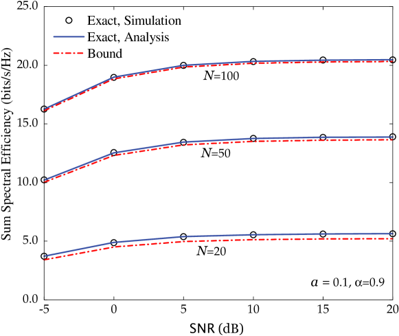
Figure 1: Sum spectral efficiency versus $\mathsf{SNR}$ for different $N(a=0.1$ and $\alpha=0.9)$.

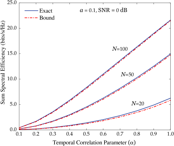
Figure 2: Sum spectral efficiency versus $\alpha$ for different $N(a=0.1$ and $\mathsf{SNR}=0\,$dB).

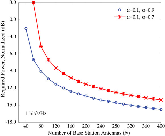
Figure 3: Transmit power required to achieve 1 bit/s/Hz per user versus $N(a=0.1$, $\alpha=0.7$ and $\alpha=0.9)$.

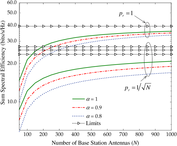
Figure 4: Sum spectral efficiency versus $N$ for different $\alpha$.

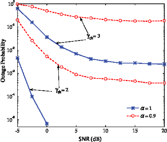
Figure 5: Outage probability versus $\mathsf{SNR}$ for different $\alpha$ and $\gamma_{\tt th}$ ($N=100$).

IV Numerical Results

In this section, we present numerical results to verify our analysis by considering a cellular network with $L=7$ cells and $K=10$ users per cell. The coherence interval is $T=200$ symbols (which corresponds to a coherence bandwidth of 200 kHz and a coherence time of 1 ms) and the length of training duration is $\tau=K$ symbols. Regarding the large-scale coefficients $\beta_{lik}$, we assume a simple scenario: $\beta_{llk}=1$ and $\beta_{lik}=a$, for $k=1,\ldots,K$, and $i\neq l$. Note that $a$ can be considered as an intercell interference factor. In all examples, we choose $a=0.1$. Furthermore, we define $\mathsf{SNR}\triangleq p_{r}$.

In the following, we will examine the sum spectral efficiency which is defined as:

$$\mathcal{S}_{l}\triangleq\left(1-\frac{\tau}{T}\right)\sum_{k=1}^{K}R_{lk}\left(p_{r},\alpha\right),$$ (43)

where $R_{lk}\left(p_{r},\alpha\right)$ is given by (21).

Figure 1 shows the sum spectral efficiency versus the SNR for $N=20$, $50$, and $100$, at the intercell interference factor $a=0.1$, and the temporal correlation parameter $\alpha=0.9$. The “Exact, Analysis” curves are computed by using (21), the “Exact, Simulation” curves are generated via (12) using Monte-Carlo simulations, while the “Bound” curves are obtained by using the bound result given in Proposition 2. The exact match between the analytical and simulated results validates our analysis. It can be seen from the figure that, the proposed bound is very tight, especially for large antenna arrays. Furthermore, we can see that, at high SNR, the sum spectral efficiency saturates. This is due to the fact that when SNR increases, both the desired signal power and intercell interference power are increased. To improve the system performance, we can use more antennas at the BS. At $\mathsf{SNR}=5$dB, the sum spectral efficiencies can be increased by the factors of $2.5$ or $5.5$ if we increase $N$ from $20$ to $50$ or from $20$ to $100$, respectively.

Next, we examine the effect of the temporal correlation parameter on the system performance as well as the tightness of our proposed bound given in Proposition 2. Figure 2 presents the sum spectral efficiency as a function of the temporal correlation parameter $\alpha$, at $\mathsf{SNR}=0$dB, for $N=20,50$, and $100$. We can see that the system performance degrades significantly when the temporal correlation parameter decreases (or the time variation in the channel increases). Half of the spectral efficiency is reduced when $\alpha$ reduces from 1 to $0.6$. Furthermore, at low $\alpha$, using more antennas at the BS does not help improve the system performance much. Regarding the tightness of the proposed bound, we can see that the bound is very tight across the entire temporal correlation range.

Figure 3 shows the transmit power, $p_{r}$, that is needed to reach $1$ bit/s/Hz per user. Here, we choose $a=0.1$ and $\alpha=0.7$ or $0.9$. As expected, the required transmit power decreases significantly when we increase the number of BS antennas. By doubling the number of BS antennas, we can cut back the transmit power by approximately $1.5$dB. This observation is in line with the results of [6].

To further verify our analysis on large antenna limits, we consider Figure 4. Figure 4 shows the sum spectral efficiency versus the number of base station antennas for different values of $\alpha$, and for two cases: the transmit power, $p_{r}$, is fixed regardless of $N$, and the transmit power is scaled as $p_{r}=1/\sqrt{N}$. The “Limits” curves are computed via the results obtained in Section III-C. As expected, as the number of the base station antennas increases, the sum spectral efficiencies converge to their limits. When the transmit power is fixed, the asymptotic performance (as $N\to\infty$) does not depend on the temporal correlation parameter. By contrast, when the transmit power is scaled as $1/\sqrt{N}$, the asymptotic performance depends on $\alpha$.

Finally, we consider the outage performance versus SNR at $N=100$, for different temporal correlation parameters ($\alpha=1$, and $0.9$), and for different threshold values ($\gamma_{\tt th}=2$, and $3$). See Figure 5. We can see that, the outage probability strongly depends on $\alpha$. At $\mathsf{SNR}=0$ dB, by reducing $\alpha$ form 1 to $0.9$, the outage probability increases from $7\times 10^{-6}$ to $5\times 10^{-3}$, and from $3\times 10^{-2}$ to $5\times 10^{-1}$ for $\gamma_{\tt th}=2$, and $3$, respectively. In addition, the outage probability significantly improves when the threshold values are slightly reduced. This is due to the fact that, with large antenna arrays, the channel hardening occurs, and hence, the SINR concentrates around its mean. As a results, by slightly reducing the threshold values, we can obtain a very low outage probability.

V Conclusions

In this paper, we characterized the uplink performance of a cellular network taking into account both the well-known pilot contamination and the unavoidable, but less studied, time variation. The latter effect, inherent in the vast majority of propagation scenarios, stems from the user mobility. Summarizing the main contributions of this work, new analytical closed-form expressions for the PDF of the SINR and the corresponding achievable sum-rate, that hold for any finite number of antennas, were derived. Moreover, a complete investigation of the low-SNR regime took place. Neveretheless, asymptotic expressions in the large antenna/user limit were also obtained, as well as the power-scaling law was studied. As a final point, numerical illustrations depicted how the time variation affects the performance in various Doppler shifts for finite and infinite number of antennas. Notably, the outcome is that large number of antennas should be preferred even in time-varying conditions.

-A Proof of Theorem 1

The uplink ergodic rate from the $k$th user in the $l$th cell to its BS (in bits/s/Hz) is given by

$$R_{lk}\!\left(\!p_{r},\alpha\!\right)\!=\!\operatorname{\mathbb{E}}_{{X_{k},Y_{k}\!\!\!}}\left\{{\!\log_{2}\!\!\left(\!\!1\!+\!\frac{p_{r}\alpha^{2}X_{k}[n-1]}{p_{r}\alpha^{2}CX_{k}[n\!-\!1]\!+\!p_{r}Y_{k}[n]\!+\!1}\!\right)}\right\}$$

$$\!=\!\int_{0}^{\infty}\!\!\!\!\int_{0}^{\infty}\!\!\!\log_{2}\left(\!1\!+\!\frac{p_{r}\alpha^{2}x}{p_{r}\alpha^{2}Cx+p_{r}y+1}\!\right)\!p_{{X_{k}}}\left({x}\right)p_{{Y_{k}}}\left({y}\right)dxdy$$

$$=\sum_{p=1}^{\varrho\left(\mathbf{\mathcal{A}}_{k}\right)}\sum_{q=1}^{\tau_{p}\left(\mathbf{\mathcal{A}}_{k}\right)}\!\frac{\mathcal{X}_{p,q}\left(\mathbf{\mathcal{A}}_{k}\right)\mu_{k,p}^{-q}\log_{2}e}{\left(q\!-\!1\right)!\left(N\!-\!K\right)!\hat{\beta}_{llk}^{N-K+1}}$$

$$\!\times\!\!\int_{0}^{\infty}\!\!\!\!\int_{0}^{\infty}\!\!\ln\!\!\left(\!\!1\!+\!\frac{p_{r}\alpha^{2}x}{p_{r}\alpha^{2}Cx\!+\!p_{r}y\!+\!1}\!\right)\!x^{N\!-\!K}e^{\frac{-x}{\hat{\beta}_{llk}}}y^{q-1}e^{\frac{-y}{\mu_{k,p}}}dxdy$$

$$=\sum_{p=1}^{\varrho\left(\mathbf{\mathcal{A}}_{k}\right)}\sum_{q=1}^{\tau_{p}\left(\mathbf{\mathcal{A}}_{k}\right)}\!\frac{\mathcal{X}_{p,q}\left(\mathbf{\mathcal{A}}_{k}\right)\mu_{k,p}^{-q}\log_{2}e}{\left(q\!-\!1\right)!\left(N\!-\!K\right)!\hat{\beta}_{llk}^{N-K+1}}$$

$$\!\times\!\bigg{(}\!\underbrace{\int_{0}^{\infty}\!\!\!\!\!\int_{0}^{\infty}\!\ln\!\!\left(\!1\!+\!\frac{p_{r}\alpha^{2}\left(\!C\!+\!1\!\right)x}{p_{r}y\!+\!1}\!\right)\!x^{N\!-\!K}e^{\frac{-x}{\hat{\beta}_{llk}}}y^{q-1}e^{\frac{-y}{\mu_{k,p}}}dxdy}_{\triangleq\mathcal{I}_{1}}$$

$$\!-\!\!\underbrace{\int_{0}^{\infty}\!\!\int_{0}^{\infty}\!\ln\left(\!1\!+\!\frac{p_{r}\alpha^{2}Cx}{\ p_{r}y\!+\!1}\!\right)\!x^{N\!-\!K}e^{\frac{-x}{\hat{\beta}_{llk}}}y^{q-1}e^{\frac{-y}{\mu_{k,p}}}dxdy}_{\triangleq\mathcal{I}_{2}}\!\!\bigg{)}\!\!\!\!$$ (44)

$$=\sum_{p=1}^{\varrho\left(\mathbf{\mathcal{A}}_{k}\right)}\sum_{q=1}^{\tau_{p}\left(\mathbf{\mathcal{A}}_{k}\right)}\!\frac{\mathcal{X}_{p,q}\left(\mathbf{\mathcal{A}}_{k}\right)\mu_{k,p}^{-q}\log_{2}e}{\left(q\!-\!1\right)!\left(N\!-\!K\right)!\hat{\beta}_{llk}^{N-K+1}}\left(\mathcal{I}_{1}-\mathcal{I}_{2}\right).$$ (45)

We first derive $\mathcal{I}_{1}$ by evaluating the integral over $x$. By using [19, Eq. (4.337.5)], we obtain

$$\mathcal{I}_{1} =\sum_{t=0}^{N-K}\!\int_{0}^{\infty}\!\left[-f(y)^{N-K-t}e^{-f(y)}\mathrm{Ei}\left(f(y)\right)\right.$$

$$\left.+\sum_{u=1}^{N-K-t}\left(u-1\right)!f(y)^{N-K-t-u}\right]y^{q-1}e^{\frac{-y}{\mu_{k,p}}}dy,$$ (46)

where $f(y)\triangleq-\frac{p_{r}y+1}{\hat{\beta}_{llk}p_{r}\alpha^{2}\left(C+1\right)}$. Using [23, Lemma 1] and [21, Eq. (39)], we can easily obtain $\mathcal{I}_{1}$ as given in (III-A). Similarly, we obtain $\mathcal{I}_{2}$ as given in (23). Substitution of $\mathcal{I}_{1}$ and $\mathcal{I}_{2}$ into (45) concludes the proof.

-B Proof of Proposition 2

By using Jensen’s inequality, we have

$$R_{lk}\left(p_{r},\alpha\right) =\operatorname{\mathbb{E}}\left\{{\log_{2}\left(1+\gamma_{k}\right)}\right\}=\operatorname{\mathbb{E}}\left\{{\log_{2}\left(1+\frac{1}{1/\gamma_{k}}\right)}\right\}$$

$$\geq\log_{2}\left(1+\frac{1}{\operatorname{\mathbb{E}}\left\{{1/\gamma_{k}}\right\}}\right)\triangleq R_{L}\left(p_{r},\alpha\right).$$ (47)

To compute $R_{L}\left(p_{r},\alpha\right)$, we need to compute $\operatorname{\mathbb{E}}\left\{{1/\gamma_{k}}\right\}$. From (16), we have

$$\operatorname{\mathbb{E}}\left\{{\frac{1}{\gamma_{k}}}\right\}=C+\frac{1}{\alpha^{2}}\sum_{i=1}^{L}\operatorname{\mathbb{E}}\left\{{\bigg{\|}\left[\hat{{\boldsymbol{G}}}_{ll}^{\dagger}[n-1]\right]_{k}\tilde{{\boldsymbol{E}}}_{li}[n]\bigg{\|}^{2}}\right\}$$

$$\hskip 99.58464pt+\frac{1}{\alpha^{2}p_{r}}\operatorname{\mathbb{E}}\left\{{\bigg{\|}\left[\hat{{\boldsymbol{G}}}_{ll}^{\dagger}[n-1]\right]_{k}\bigg{\|}^{2}}\right\}$$

$$\!=\!C\!+\!\frac{1}{\alpha^{2}}\!\!\operatorname{\mathbb{E}}\left\{{\bigg{\|}\!\!\left[\!\hat{{\boldsymbol{G}}}_{ll}^{\dagger}[n\!-\!1]\!\right]_{k}\!\bigg{\|}^{2}}\right\}\!\!\left(\sum_{i=1}^{L}\!\sum_{k=1}^{K}\!\left(\!\beta_{lik}\!-\!\alpha^{2}\hat{\beta}_{lik}\!\right)\!+\!\frac{1}{p_{r}}\!\right)$$

$$\!=\!C\!+\!\frac{1}{\left(\!N\!-\!K\!\right)\!\alpha^{2}\hat{\beta}_{llk}}\left(\sum_{i=1}^{L}\sum_{k=1}^{K}\!\left(\beta_{lik}\!-\!\alpha^{2}\hat{\beta}_{lik}\!\right)\!+\!\frac{1}{p_{r}}\right).$$ (48)

In the third equality of (48), we have considered the independence between the two variables, while in the last equality, we have used the following result:

$$\operatorname{\mathbb{E}}\left\{{\bigg{\|}\left[\hat{{\boldsymbol{G}}}_{ll}^{\dagger}[n-1]\right]_{k}\bigg{\|}^{2}}\right\}=\operatorname{\mathbb{E}}_{{X_{k}}}\left\{{\frac{1}{X_{k}[n-1]}}\right\}$$

$$\!=\!\int_{0}^{\infty}\!\!\!\frac{e^{-x/\hat{\beta}_{llk}}}{\left(N-K\right)!\hat{\beta}_{llk}^{2}}\!\!\left(\frac{x}{\hat{\beta}_{llk}}\right)^{N\!-\!K\!-\!1}\!\!\!\mathrm{d}x=\frac{1}{\left(N-K\right)\hat{\beta}_{llk}}.$$ (49)

Note that we have used [19, Eq. (3.326.2)] to obtain (49). Thus, the desired result (2) is obtained from (-B) and  (48).

-C Proof of Theorem 2

Clearly, from (13), $\gamma_{k}<1/C$. Thus, if $\gamma_{{\tt th}}\geq 1/C$, then $P_{{\tt out}}\left(\gamma_{{\tt th}}\right)=1$. Next, we consider the case where $\gamma_{{\tt th}}<1/C$. Taking the probability of the instantaneous SINR $\gamma_{k}$, given by (13), we can determine the outage probability as

$$P_{{\tt out}}\!=\!{\tt Pr}\left(\frac{\alpha^{2}p_{r}X_{k}}{\alpha^{2}p_{r}CX_{k}+p_{r}Y_{k}+1}\leq\gamma_{{\tt th}}\right)$$

$$\!=\!\int_{0}^{\infty}{\tt Pr}\left(X_{k}<\frac{\gamma_{{\tt th}}\left(p_{r}Y_{k}+1\right)}{\alpha^{2}p_{r}-\gamma_{{\tt th}}\alpha^{2}p_{r}C}\left.\right|Y_{k}\right)p_{Y_{k}}(y)\mathrm{d}y$$

$$\!=\!1\!-\!e^{\frac{-\gamma_{{\tt th}}}{p_{r}\bar{\gamma}_{{\tt th}}}}\!\sum^{N-K}_{t=0}\!\!\int_{0}^{\infty}\!\!\!e^{\frac{-y}{\bar{\gamma}_{{\tt th}}}}\!\sum^{N-K}_{t=0}\!\!\frac{\left(\frac{\gamma_{{\tt th}}}{\bar{\gamma}_{{\tt th}}}\right)^{\!\!t}}{t!}\!\left(\!y\!+\!\frac{1}{p_{r}}\!\right)^{\!\!t}\!\!p_{Y_{k}}(y)\mathrm{d}y$$

$$\!=\!1\!-\!e^{\frac{-\gamma_{{\tt th}}}{p_{r}\bar{\gamma}_{{\tt th}}}}\sum_{p=1}^{\varrho\left(\mathbf{\mathcal{A}}_{k}\right)}\sum_{q=1}^{\tau_{p}\left(\mathbf{\mathcal{A}}_{k}\right)}\sum_{t=0}^{N-K}\mathcal{X}_{p,q}\left(\mathbf{\mathcal{A}}_{k}\right)\frac{\mu_{k,p}^{-q}}{\left(q-1\right)}\frac{\left(\frac{\gamma_{{\tt th}}}{\bar{\gamma}_{{\tt th}}}\right)^{t}}{t!}$$

$$\hskip 85.35826pt\times\int_{0}^{\infty}y^{q-1}e^{\frac{-y}{\bar{\gamma}_{{\tt th}})}}\left(y+\frac{1}{p_{r}}\right)^{t}\mathrm{d}y$$

$$\!=\!1\!-\!e^{\frac{-\gamma_{{\tt th}}}{p_{r}\bar{\gamma}_{{\tt th}}}}\!\!\sum_{p=1}^{\varrho\left(\mathbf{\mathcal{A}}_{k}\right)}\!\sum_{q=1}^{\tau_{p}\left(\mathbf{\mathcal{A}}_{k}\right)}\!\sum_{t=0}^{N-K}\!\!\sum_{s=0}^{t}\!\!\binom{t}{s}\mathcal{X}_{p,q}\!\left(\mathbf{\mathcal{A}}_{k}\!\right)\!\frac{\Gamma\left(s\!+\!q\right)\!\bar{\gamma}_{{\tt th}}^{s+q}}{\mu_{k,p}^{q}\left(q\!-\!1\right)},$$ (50)

where $\bar{\gamma}_{{\tt th}}\triangleq\hat{\beta}_{llk}\left(\alpha^{2}-\alpha^{2}C\gamma_{{\tt th}}\right)$, and where in the third equality, we have used that the cumulative density function of $X_{k}$ (Erlang variable) is

$$F_{X_{k}}(x) ={\tt Pr}\left(X_{k}\leq x\right)$$

$$=1-\exp\left(-\frac{x}{\hat{\beta}_{llk}}\right)\sum_{t=0}^{N-K}\frac{1}{t!}\left(\frac{x}{\hat{\beta}_{llk}}\right)^{t}.$$ (51)

The last equality of (50) was derived after applying the binomial expansion of $(y+1/p_{r})^{t}$ and [19, Eq. (3.351.1)].

$$\!\!\!\!\ddot{R}_{lk}\left(p_{r},\alpha\right)=\frac{1}{\mathrm{ln}2}\operatorname{\mathbb{E}}_{{X_{k},Y_{k}}}\left\{{\frac{\alpha^{2}X_{k}[n-1]\left(\alpha^{4}X_{k}^{2}[n-1]+2\varsigma_{k}\left(1+p_{r}\varsigma_{k}\right)^{2}\left(1+\alpha^{2}p_{r}X_{k}[n-1]+p_{r}\varsigma_{k}\right)\right)}{\left(\alpha^{4}p_{r}^{2}\left(C+1\right)X_{k}^{2}[n-1]+pY_{k}[n]+1\right)^{2}\left(\alpha^{4}p_{r}^{2}CX_{k}^{2}[n-1]+p_{r}Y_{k}[n]+1\right)^{4}}}\right\},$$ (56)

-D Proof of Theorem 3

The initial step for the derivation of the minimum transmit energy per information bit is to cover the need for exact expressions regarding the derivatives of ${R}_{lk}\left(p_{r},\alpha\right)$. In particular, this can be given by

$$\!\!\dot{R}_{lk}\left(\!p_{r},\alpha\!\right)\!=\!\frac{1}{\mathrm{ln}2}$$

$$\!\!\!\!\times\!\operatorname{\mathbb{E}}_{{X_{k},Y_{k}\!\!\!}}\left\{{\!\!\frac{\alpha^{2}X_{k}[n\!-\!1]\big{/}\!\!\left(\!\alpha^{4}p_{r}^{2}CX_{k}^{2}[n\!-\!1]\!+\!p_{r}Y_{k}[n]\!+\!1\!\right)\!\!}{\left(\!\alpha^{4}p_{r}^{2}\left(\!C\!+\!1\!\right)\!X_{k}^{2}[n-1]\!+\!p_{r}Y_{k}[n]+1\!\right)}}\right\}\!\!.$$ (52)

Easily, its value at $p_{r}=0$ is

$$\dot{R}_{lk}\left(0,\alpha\right)=\frac{1}{\mathrm{ln}2}\operatorname{\mathbb{E}}_{{X_{k}}}\left\{{\alpha^{2}X_{k}[n-1]}\right\}.$$ (53)

Taking into account that $X_{k}[n-1]$ is Erlang distributed, its expectation can be written as

$$\operatorname{\mathbb{E}}_{{X_{k}}}\left\{{X_{k}[n-1]}\right\}=\left(N-K+1\right)\hat{\beta}_{llk}.$$ (54)

Substituting (54) and (53) into (31), we obtain the desired result.

The second derivative of ${R}_{lk}\left(p_{r},\alpha\right)$, needed for the evaluation of the wideband slope, is given by (56) shown at the top of the previous page, where $\varsigma_{k}\triangleq\alpha^{2}CX_{k}[n-1]+Y_{k}[n]$. Hence, $\ddot{R}_{lk}\left(0,\alpha\right)$ can be expressed by

$$\ddot{R}_{lk}\left(0,\alpha\right) =\frac{1}{\mathrm{ln}2}\mathbb{E}_{X_{k},Y_{k}}\left\{\alpha^{6}X_{k}^{3}[n-1]+2\alpha^{4}CX_{k}^{2}[n-1]\right.$$

$$\hskip 71.13188pt\left.+2\alpha^{2}X_{k}[n-1]Y_{k}[n]\right\}.$$ (57)

The moments of $X_{k}[n-1]$ are obtained by means of the corresponding derivatives of its moment generating function (MGF) at zero $\mathrm{M}_{X_{k}}^{\left(n\right)}\left(0\right)$, i.e., $\operatorname{\mathbb{E}}_{{X_{k}}}\left\{{X_{k}^{n}[n-1]}\right\}=\mathrm{M}_{X_{k}}^{\left(n\right)}\left(0\right)$. Thus, having in mind that the MGF of the Erlang distribution is

$$\mathrm{M}_{X_{k}}\left(t\right)=\frac{1}{\left(1-\hat{\beta}_{llk}t\right)^{N-K+1}},$$ (58)

we can obtain the required moments of $X_{k}[n-1]$ as

$$\operatorname{\mathbb{E}}_{{X_{k}}}\left\{{X_{k}^{2}[n-1]}\right\} =\mathrm{M}_{X_{k}}^{\left(2\right)}\left(0\right)$$

$$=\frac{\Gamma\left(N-K+3\right)}{\Gamma\left(N-K+1\right)}\hat{\beta}_{llk}^{2}$$ (59)

$$\operatorname{\mathbb{E}}_{{X_{k}}}\left\{{X_{k}^{3}[n-1]}\right\} =\mathrm{M}_{X_{k}}^{\left(3\right)}\left(0\right)$$

$$=\frac{\Gamma\left(N-K+4\right)}{\Gamma\left(N-K+1\right)}\hat{\beta}_{llk}^{3}.$$ (60)

In addition, since $X_{k}[n-1]$ and $Y_{k}[n]$ are uncorrelated, we have $\operatorname{\mathbb{E}}_{{X_{k},Y_{k}}}\left\{{X_{k}[n-1]Y_{k}[n]}\right\}=\operatorname{\mathbb{E}}_{{X_{k}}}\left\{{X_{k}[n-1]}\right\}\operatorname{\mathbb{E}}_{{Y_{k}}}\left\{{Y_{k}[n]}\right\}$. In other words, it is necessary to find the expectation of $Y_{k}[n]$. As aforementioned, the PDF of $Y_{k}[n]$ obeys (15) and has expectation given by definition as

$$\operatorname{\mathbb{E}}_{{Y_{k}}}\left\{{Y_{k}[n]}\right\} =\int_{0}^{\infty}yp_{{Y_{k}}}\left({y}\right)\mathrm{d}y$$

$$=\sum_{p=1}^{\varrho\left(\mathbf{\mathcal{A}}_{k}\right)}\sum_{q=1}^{\tau_{p}\left(\mathbf{\mathcal{A}}_{k}\right)}\!\!\!\mathcal{X}_{p,q}\left(\mathbf{\mathcal{A}}_{k}\right)\frac{\mu_{k,p}^{-q}}{\left(q-1\right)!}\int_{0}^{\infty}\!\!\!y^{q}e^{\frac{-y}{\mu_{k,p}}}\mathrm{d}y$$

$$=\sum_{p=1}^{\varrho\left(\mathbf{\mathcal{A}}_{k}\right)}\sum_{q=1}^{\tau_{p}\left(\mathbf{\mathcal{A}}_{k}\right)}\!\mathcal{X}_{p,q}\left(\mathbf{\mathcal{A}}_{k}\right)\frac{\mu_{k,p}^{-q}q}{\left(q-1\right)!},$$ (61)

where we have used [19, Eq. (3.326.2)] as well as the identity $\Gamma\left(q+1\right)=q!$. As a result, $\ddot{R}_{lk}\left(0,\alpha\right)$ follows by means of (-D), (60), (61). Finally, substitution of the (53) and (-D) into (32) yields the wideband slope.

References

• [1] A. Papazafeiropoulos, H. Q. Ngo, M. Matthaiou, and T. Ratnarajah, “Uplink performance of conventional and massive MIMO cellular systems with delayed CSIT,” in Proc. IEEE International Symposium on Personal, Indoor and Mobile Radio Communications (PIMRC), Washington, D.C., Sep. 2014.
• [2] “5G: A Technology Vision,” Huawei Technologies Co., Ltd., Shenzhen, China, Whitepaper, Nov. 2013. [Online]. www.huawei.com/ilink/en/download/HW_314849
• [3] D. Gesbert, M. Kountouris, R. W. Heath Jr., C. B. Chae, and T. Sälzer, “Shifting the MIMO paradigm,” IEEE Sig. Proc. Mag., vol. 24, no. 5, pp. 36–46, Oct. 2007.
• [4] T. L. Marzetta, “Noncooperative cellular wireless with unlimited numbers of base station antennas,” IEEE Trans. Wireless Commun., vol. 9, no. 11, pp. 3590–3600, Nov. 2010.
• [5] E. G. Larsson, F. Tufvesson, O. Edfors, and T. L. Marzetta, “Massive MIMO for next generation wireless systems,” IEEE Commun. Mag., vol. 52, no. 2, pp. 186–195, Feb. 2014.
• [6] H. Q. Ngo, E. G. Larsson, and T. L. Marzetta, “Energy and spectral efficiency of very large multiuser MIMO systems,” IEEE Trans. Commun., vol. 61, no. 4, pp. 1436–1449, Apr. 2013.
• [7] C. J. Chen and L. C. Wang, “Performance analysis of scheduling in multiuser MIMO systems with zero-forcing receivers,” IEEE J. Sel. Areas Commun., vol. 25, no. 7, pp. 1435–1445, Sep. 2007.
• [8] G. Caire and S. Shamai (Shitz), “On the achievable throughput of a multiantenna Gaussian broadcast channel,” IEEE Trans. Inf. Theory, vol. 49, no. 7, pp. 1691–1706, Jul. 2006.
• [9] J. Jose, A. Ashikhmin, T. L. Marzetta, and S. Vishwanath, “Pilot contamination and precoding in multi-cell TDD systems,” IEEE Trans. Wireless Commun., vol. 10, no. 8, pp. 2640–2651, Aug. 2011.
• [10] K. T. Truong and R. W. Heath, Jr., “Effects of channel aging in Massive MIMO Systems,” IEEE/KICS J. Commun. Netw., vol. 15, no. 4, pp. 338–351, Aug. 2013.
• [11] A. Papazafeiropoulos and T. Ratnarajah “Linear precoding for downlink massive MIMO with delayed CSIT and channel prediction” in Proc. IEEE WCNC 2014, Apr. 2014, pp. 821–826.
• [12] A. Papazafeiropoulos and T. Ratnarajah “Uplink performance of massive MIMO subject to delayed CSIT and anticipated channel prediction,” in Proc. IEEE ICASSP, May 2014.
• [13] H. Q. Ngo, M. Matthaiou, T. Q. Duong, and E. G. Larsson, “Uplink performance analysis of multicell MU-SIMO systems with ZF receivers,” IEEE Trans. Veh. Tech., vol. 62, no. 9, pp. 4471–4483, Nov. 2013.
• [14] S. Verdú, Multiuser Detection.   Cambridge, UK: Cambridge University Press, 1998.
• [15] H. Q. Ngo, M. Matthaiou, and E. G. Larsson. “Performance analysis of large scale MU-MIMO with optimal linear receivers,” in Proc. IEEE Swe-CTW, Oct. 2012, pp. 59–64.
• [16] H. Shin and M. Z. Win, “MIMO diversity in the presence of double scattering,” IEEE Trans. Inf. Theory, vol. 54, no. 7, pp. 2976–2996, Jul. 2008.
• [17] D. A. Gore, R. W. Heath Jr., and A. J. Paulraj, “Transmit selection in spatial multiplexing systems,” IEEE Commun. Lett., vol. 6, no. 11, pp. 491–493, Nov. 2002.
• [18] A. Bletsas, H. Shin, and M. Z. Win, “Cooperative communications with outage-optimal opportunistic relaying,” IEEE Trans. Wireless Commun., vol. 6, no. 9, pp. 3450–3460, Sep. 2007.
• [19] I. S. Gradshteyn and I. M. Ryzhik, Table of Integrals, Series, and Products, 7th ed.   San Diego, CA: Academic, 2007.
• [20] Wolfram, “The Wolfram functions site.” Available: http://functions.wolfram.com
• [21] M. Kang and M.-S. Alouini, “Capacity of MIMO Rician channels,” IEEE Trans. Wireless Commun., vol. 5, no. 1, pp. 112–122, Jan. 2006.
• [22] A. P. Prudnikov, Y. A. Brychkov, and O. I. Marichev, Integrals and Series, Volume 3: More Special Functions.   New York: Gordon and Breach Science, 1990.
• [23] H. Q. Ngo, T. Q. Duong, and E. G. Larsson, “Uplink performance analysis of multicell MU-MIMO with zero-forcing receivers and perfect CSI,” in Proc. IEEE Swe-CTW, Sweden, Nov. 2011, pp. 40–45.
• [24] S. Verdú, “Spectral effciency in the wideband regime,” IEEE Trans. Info. Theory, vol. 48, no. 6, pp. 1319–1343, Jun. 2002.
• [25] P. Billingsley, Probability and Measure, 3rd ed. John Wiley & Sons, Inc., 1995.
• [26] A. W. van der Vaart, Asymptotic Statistics (Cambridge Series in Statistical and Probabilistic Mathematics). Cambridge University Press, New York, 2000.
• [27] S. Shamai (Shitz) and S. Verdú, “The impact of frequency-flat fading on the spectral efficiency of CDMA,” IEEE Trans. Inf. Theory, vol. 47, no. 4, pp. 1302–1327, May 2001.
• [28] A. Lozano, A. M. Tulino, and S. Verdú, “High–SNR power offset in multiantenna communications,” IEEE Trans. Inf. Theory, vol. 51, no. 12, pp. 4134–4151, Dec. 2005.
• [29] Wolfram, “The Wolfram functions site.” Available: http://functions.wolfram.com