Rotation of a spheroid in a simple shear at small Reynolds number
Abstract
We derive an effective equation of motion for the orientational dynamics of a neutrally buoyant spheroid suspended in a simple shear flow, valid for arbitrary particle aspect ratios and to linear order in the shear Reynolds number. We show how inertial effects lift the degeneracy of the Jeffery orbits and determine the stabilities of the log-rolling and tumbling orbits at infinitesimal shear Reynolds numbers. For prolate spheroids we find stable tumbling in the shear plane, log-rolling is unstable. For oblate particles, by contrast, log-rolling is stable and tumbling is unstable provided that the aspect ratio is larger than a critical value. When the aspect ratio is smaller than this value tumbling turns stable, and an unstable limit cycle is born.
pacs:
83.10.Pp,47.15.G-,47.55.Kf,47.10.-gI Introduction
In this article we describe the effect of weak inertia upon the orientational dynamics of a neutrally buoyant spheroid in a simple shear flow using perturbation theory. In the absence of inertial effects the rotation of a neutrally buoyant spheroid in a simple shear was determined by Jeffery who found that there are infinitely many degenerate periodic orbitsJeffery (1922), the so-called ‘Jeffery orbits’. In this limit the initial orientation determines in which way the particle rotates. Fluid and particle inertia lift this degeneracy, but little is known about how this comes about. A notable exception is the work by Subramanian and Koch who have solved the problem for rod-shaped particles in the slender-body approximation Subramanian and Koch (2005). We discuss other theoretical results below in Section II.
The question is currently of great interest: several recent papers have reported results of direct numerical simulations (DNS) of the problem, using ‘lattice Boltzmann’ methods Qi and Luo (2003); Huang et al. (2012); Rosén, Lundell, and Aidun (2014); Mao and Alexeev (2014). These studies reveal that fluid and particle inertia affect the orientational dynamics of a neutrally buoyant spheroid in a simple shear in intricate ways. The DNS are performed at moderate and large shear Reynolds numbers, defined as where is the largest particle dimension, is the shear strength and the kinematic viscosity of the suspending fluid. DNS at very small Reynolds numbers are difficult to perform. But this limit ( of order unity and smaller) is of particular interest. There is a long-standing question whether or not a nearly spherical prolate spheroid exhibits stable ‘log-rolling’ in this limit, so that its symmetry axis aligns with the vorticity axis. It was first suggested by Saffman that this is the case Saffman (1956), in an attempt to explain Jeffery’s hypothesisJeffery (1922) that spheroids rotate in orbits that minimise energy dissipation. But stable log-rolling of prolate spheroids has not been found in DNS, and it has been suggested that higher -corrections may explain this discrepancyMao and Alexeev (2014). The small- limit is of interest also because it provides stringent tests for DNS.
These reasons motivated us to derive an equation of motion that takes into account the effect of weak fluid and particle inertia. Our main result is an approximate dynamical equation for the rotation of a neutrally buoyant spheroid suspended in a simple shear flow, valid for arbitrary aspect ratios and to first order in (Eq. (42) in Section IV). In the slender-body limit this equation is of the same form as the one derived in Ref. 2. In the completely inertia-free case our results reduce to Jeffery’s equationJeffery (1922). We find that corrections to this limit arise from both particle inertia (centrifugal and gyroscopic forces), as well as from fluid inertia (modifying the hydrodynamic torque on the particle). The particle-inertia corrections we report here are consistent with earlier numerical and analytical resultsLundell and Carlsson (2010); Einarsson, Angilella, and Mehlig (2014).
Fluid-inertia corrections are taken into account to first order in using a reciprocal theoremKim and Karrila (1991). Our approach is similar to the one adopted in Ref. 2 in the slender-body limit, but our equation of motion is valid for spheroids with arbitrary aspect ratios. By linear stability analysis we determine the stabilities of the periodic orbits of this equation at infinitesimal as a function of the particle aspect ratio. The stability calculation details how the degeneracy of the Jeffery orbits for a neutrally buoyant spheroid in a simple shear is lifted by weak inertia.
We find that the log-rolling orbit is unstable for prolate particles. This explains why stable log-rolling is not observed in DNSQi and Luo (2003); Huang et al. (2012); Rosén, Lundell, and Aidun (2014); Mao and Alexeev (2014) at the smallest shear Reynolds numbers accessible in the simulations. Moreover we find that tumbling in the flow-shear plane is stable for prolate particles. As the aspect ratio tends to unity there is a bifurcation: for nearly spherical oblate particles log-rolling is stable and tumbling in the flow-shear plane is unstable. There is a second bifurcation for oblate particles. At a critical aspect ratio tumbling becomes stable and an unstable limit cycle is born. This means that the behaviour of a very flat disk depends on its initial orientation for . We discuss how the shape of the limit cycle changes as the aspect ratio tends to zero.
The remainder of this article is organised as follows. In Section II we give an overview over the background of the problem. Section III summarises the method employed in this article, based on a reciprocal theorem Kim and Karrila (1991). We demonstrate how to calculate the effect of particle and fluid inertia to first order, and how we use the symmetries of the problem to make it tractable. Section IV summarises our results: the equation of motion and its stability analysis. We discuss the results in Section V and conclude with Section VI.
A brief account of the main results described in this article was given in Ref. 11. Here we describe the complete derivation. We also present additional results and discussion that could not be included in the shorter format: we quote precise asymptotic formulae for small and large aspect ratios, as well as for aspect ratios close to unity. We also characterise the limit cycle that arises for , and compute its linear stability.
II Background
The question of describing the rotation of a neutrally buoyant particle in a simple shear flow has a long history. Jeffery derived an expression for the torque on an ellipsoidal (tri-axial) particle neglecting inertial effects Jeffery (1922). To obtain an equation of motion for small particles he assumed that the dynamics is overdamped, that the particle rotates so as to instantaneously achieve zero torque. This gives rise to Jeffery’s equation that is commonly quoted for the special case of spheroidal (axisymmetric) particles. From this equation it follows that spheroids suspended in a simple shear tumble, they stay aligned with the flow direction for some time and then switch orientation by degrees. The dynamics is degenerate in that there are infinitely many different periodic orbits, the so-called ‘Jeffery orbits’. The initial orientation determines which particular orbit is selected. The goal of Jeffery’s calculation was to compute the viscosity of a dilute suspension of spheroids, and Jeffery hypothesised that the particles select orbits that minimise energy dissipation.
SaffmanSaffman (1956) pointed out that inertial effects lift the degeneracy of the Jeffery orbits, and he described the orientational dynamics of a nearly spherical particle in a simple shear taking into account fluid inertia. For prolate particles he concluded that log-rolling is stable, that tumbling in the shear plane is unstable, and that the stabilities are reversed for oblate particles. These results are stated in terms of an effective drift for the particle orientation (towards the vorticity axis for prolate particles). This conclusion supports Jeffery’s hypothesis. Saffman did not take into account particle inertia. His method of calculation rests on a joint expansion in small eccentricity and .
Harper & ChangHarper and Chang (1968) addressed the problem in a different way, modeling the dynamics of a rod in a simple shear in terms a dumb-bell, that is two spheres connected by an invisible rigid rod. The spheres are subject to Stokes drag and hydrodynamic lift forcesSaffman (1965). This approximation neglects hydrodynamic interactions between the two spheres, as well as the unsteady term in the Navier-Stokes equations. Harper & Chang arrive at the opposite conclusion, namely that log-rolling is unstable. Since their result pertains to the slender-body limit the question is how the stability of the log-rolling orbit depends on the particle aspect ratio.
It was subsequently shown by Hinch & LealHinch and Leal (1972) how weak rotational diffusion breaks the degeneracy of the Jeffery orbits, and their results form the basis for a large part of the work during the last decades on the rheology of dilute suspensions, see Refs. 15 and 16 for reviews.
Recently there has been a surge of interest in determining the effect of weak inertia upon a spheroid tumbling in a simple shear flow in the absence of rotational diffusion. Subramanian & KochSubramanian and Koch (2005) derived an effective equation of motion for a neutrally buoyant rod in the slender-body limit to first order in fluid and particle inertia. Their calculation uses a reciprocal theoremKim and Karrila (1991) and takes into account the unsteady term in the Navier Stokes equation as well as particle inertia. The authors arrive at qualitatively the same conclusion as Harper & Chang, namely that the orientation of the rod eventually drifts towards the flow-shear plane.
In a second paper Subramanian & KochSubramanian and Koch (2006) repeated Saffman’s calculation for a neutrally buoyant nearly spherical particle. They used a different method, similar to the one used in Ref. 2, and come to the same conclusion as Saffman, that log-rolling is stable for nearly-spherical prolate particles.
Recent DNSQi and Luo (2003); Huang et al. (2012); Rosén, Lundell, and Aidun (2014); Mao and Alexeev (2014) have explored the stability of log-rolling and tumbling orbits, mostly at moderate and large Reynolds numbers, and only for a small number of aspect ratios. The simulations show unstable log-rolling for prolate particles at the smallest Reynolds numbers studied. We note that You, Phan-Thien & TannerYu, Phan-Thien, and Tanner (2007) misquote Saffman when they describe their numerical results on the rotation of a spheroid in a Couette flow at Reynolds numbers of the order of and larger. In the introduction of Ref. 18 it is implied that Saffman’s theorySaffman (1956) predicts that nearly spherical prolate particles tend to the flow-shear plane.
III Method
In this section we give a brief but complete summary of our calculation. The most technical details and tabulations are deferred to appendices. We start with notation and the relevant dimensionless parameters determining the physics. Then we give the governing equations and explain how to express the hydrodynamic torque through a reciprocal theoremLorentz (1896); Happel and Brenner (1983); Kim and Karrila (1991); Subramanian and Koch (2005). Finally we explain the perturbation scheme and list the symmetries that severely constrain the form of the solution.
III.1 Notation
The calculations described in this paper involve vectors and tensors in three spatial dimensions. We employ index notation with the implicit summation convention for repated indices, and we use the Kronecker () and Levi-Civita () tensors.
III.2 Units and dimensionless numbers
The physics of the problem is governed by three dimensionless numbers: the shear Reynolds number (measuring fluid inertia), the Stokes number St (measuring particle inertia) and the particle aspect ratio .
We work with dimensionless variables. The length scale is given by the particle major axis . The velocity scale is taken to be where is the shear rate. The explicit time dependence of the flow (the time scale for the unsteady fluid inertia) scales as since it is determined by the particle angular velocity because to lowest order the unsteadiness arises from the particle motion. The corresponding scale for pressure is , and force and torque are measured in units of and , respectively.
From these scales the dimensionless parameters are formed. As mentioned in the Introduction, the shear Reynolds number is defined as
| (1) |
Here is the density and is the dynamic viscosity of the surrounding fluid ( is the kinematic viscosity).
The Stokes number, measuring the particle inertia, is given by the ratio of the typical rate of change of angular momentum and the typical torque:
| (2) |
Here is the particle density. For a neutrally buoyant particle, , we have .
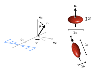
We define the particle aspect ratio as the ratio between the length along the symmetry axis and the length transverse to the symmetry axis (Fig. 1). That is denotes prolate particles while denotes oblate particles. Because we measure length in units of the major particle axis , the aspect ratio of a prolate particle is , while the aspect ratio of an oblate particle is , where denotes the length of the minor axis of the particle (see Fig. 1).
III.3 Equations of motion
Let denote the components of the unit vector pointing in the direction of the particle symmetry axis (Fig. 1), and the components of the angular velocity of the particle. Newton’s second law for the orientational degrees of freedom for an axisymmetric particle reads:
| (3) |
Dots denote time derivatives, and are the elements of the moment-of-inertia tensor of the particle, and is the torque exerted on the particle. The moment-of-inertia tensor of an axisymmetric particle with axis of symmetry is on the form
| (4) |
where and correspond to the moments-of-inertia around and transverse to the symmetry axis. Using the dimensionless variables introduced in Section III.2 we have for a prolate spheroid ()
| (5) |
and for an oblate spheroid ()
| (6) |
We rewrite the equation of motion (3) as
| (7) |
In the final step we used the definition (4) of and the equation of motion (3) for .
III.4 Calculation of the hydrodynamic torque to order
The straightforward approach to determine the torque on a particle in a fluid is to solve Navier-Stokes equations for the velocity and pressure fields, then compute the stress tensor and finally integrate the stress tensor over the surface of the particle. The reciprocal theoremLorentz (1896); Kim and Karrila (1991); Subramanian and Koch (2005) offers an alternative, and often more convenient, route to the hydrodynamic forces. In particular, we may avoid solving for the complete flow field. In this Section we specify the Navier-Stokes problem we need to solve, and explain how we use the reciprocal theorem to simplify the calculations.
Navier-Stokes problem for the disturbance flow. We consider a particle with boundary immersed in an linear ambient flow . Throughout this paper we express the ambient flow as
| (8) |
or equivalently with
| (9) |
Here and are the symmetric and antisymmetric parts of the flow gradient, given by
| (10) |
In dimensionless variables (Section III.2) the Navier-Stokes equations read
| (11) |
Note that the unsteady and convective inertia terms come with the same prefactor in this problem. This happens because the timescale of the particle motion is the same as the timescale of the flow. The boundary condition is no-slip on the surface of the particle
| (12) |
We introduce the disturbance field from the particle
| (13) |
If we assume that satisfies the Navier-Stokes equations we have the disturbance problem
| (14) |
and the boundary conditions is expressed in the slip angular velocity as
| (15) |
Finally, when applying the reciprocal theorem we shall use that, by definition, the divergence of the stress tensor satisfies the following equalities:
| (16) |
The Stokes solution. This paper concerns a spheroidal particle suspended in a linear flow. We thus need explicit solutions to Eq. (14) at in this geometry. We use a finite multipole expansionChwang and Wu (1975); Kim and Karrila (1991) (see Appendix A). In our notation they read
| (17) | ||||
where
Here , , , , , and are known constants that depend on the particle aspect ratio . The exact definition of the spheroidal multipoles and the values of all constants are given in Appendix A, see in particular Table 3.
The reciprocal theorem. This theoremLorentz (1896); Happel and Brenner (1983); Kim and Karrila (1991); Subramanian and Koch (2005) relates integrals of the velocity and stress fields of two incompressible and Newtonian fluids. The idea is the following. Let one set of fields represent the actual problem of interest, the primary problem. Then choose the second set of fields to be an auxiliary problem with known solution, such that an integral in the theorem relates to hydrodynamic torque of the primary problem. Provided that all integrals in the theorem converge and can be evaluated, we can solve the resulting equations for the hydrodynamic torque.
The reciprocal theorem for the two sets and can be stated as
| (18) |
Here is the differential force from the fluid on the surface element with normal vector . The volume integrals are to be taken over the entire fluid volume outside the particle, and the surface integrals over all surfaces bounding the fluid volume, with surface normals pointing out of the fluid volume.
In the following we apply the reciprocal theorem to the calculation of the hydrodynamic torque on a particle.
Calculation of the torque. We choose the auxiliary problem to be the Stokes flow around an identical particle rotating with an angular velocity in an otherwise quiescent fluid. Its solution is given by Eq. (17) with . The primary problem is the disturbance problem defined in Eq. (14). Inserting the boundary conditions into the reciprocal theorem yields
| (19) |
We also used that . This equality holds because is a Stokes flow. Both primary and auxiliary velocity fields vanish as , therefore both integration surfaces are only the particle surface . Note that the surface integrals are to be taken with surface normals out of the fluid domain, so that is the differential force exerted on the particle by the fluid. In the integrals we identify the hydrodynamic torque on the particle, it is given by
| (20) |
It follows:
| (21) |
The auxiliary torque together with the surface integral add up to the Jeffery torqueJeffery (1922) :
| (22) |
The constant is given in Table 3 in Appendix A. The contribution
| (23) |
evaluates to zero for any linear flow . It follows that Eq. (21) becomes
| (24) |
Since is linear in , this variable can be eliminated. We finally obtain:
| (25) |
where
| (26) | ||||
Thus far we have made no approximation, and Eq. (25) is exact, the difficulty lies in evaluating the Navier-Stokes disturbance flow . This is a complicated non-linear problem since , and all depend on the direction and upon the angular velocity of the particle. The flow equations thus couple non-linearly to the rigid body equations of motion for the particle. In the following we solve this system of equations in perturbation theory valid to first order in St and .
III.5 Perturbative calculation of the particle angular velocity
In this section we determine the angular velocity of the particle to lowest order in St and , assuming that both St and are small, so that is negligible. We recall the equation of motion (7) for the particle orientation, and insert the expression for the hydrodynamic torque obtained in Section III.4:
| (27) |
Now we expand the angular velocity as
| (28) |
Next, we insert these expansions into the equation of motion (7) and collect terms of equal order in St and :
| (29) |
In the last term it is understood that the volume integral need only be evaluated to , so that we may use the Stokes flow solutions for . The first equation gives the Jeffery angular velocity ,
| (30) |
The dynamics of is to lowest order given by
| (31) |
From Table 3 in Appendix A we infer that for both prolate and oblate spheroids
| (32) |
This shows that Eq. (31) is Jeffery’s equationJeffery (1922) for the orientational dynamics of a spheroid in a simple shear.
The two remaining equations in (29) may be inverted to
| (33) |
Eq. (28) together with Eqs. (30) and (33) yield the effective angular velocity under the effect of weak particle and fluid inertia. From the equation of motion (7) we define the effective vector field
| (34) |
This vector field describes the time evolution of . The first term is the Jeffery vector field (31). The two new terms represent the effects of particle inertia and fluid inertia. The terms due to particle inertia are straightforward to evaluate directly, but the volume integral in Eq. (33) is very tedious to evaluate. To make the calculation feasible we exploit the symmetries of the problem.
III.6 Symmetries of the effective equation of motion
Both correction terms in Eq. (34) are quadratic in the ambient flow gradient tensor . In other words, they are on the form
| (35) |
where the tensorial coefficients are composed of the remaining available tensor quantities: and ( is already used in ). We make an exhaustive enumeration of all possible combinations, and then use the symmetries listed in Table 1 to remove or combine items in the list. For example we start by letting
| (36) |
where the sum is over all permutations of , and are unique coefficients for each term. We include only odd powers of as any even terms would break the particle inversion symmetry. We then insert this enumeration into the first term of Eq. (35), and contract and apply the first three symmetries in Table 1 until we reach a list of unique candidate terms. In this case the only two unique terms turn out to be and . Finally, we use the fact that the equation of motion may not change the magnitude of the unit vector . This constraint forces the coefficients of the two unique terms to be the same magnitude but opposite sign. Upon renaming the coefficients we get the first term in Eq. (37). The other terms are derived similarly by inserting (36) into the other terms in Eq. (35). The result contains only six independent terms:
| (37) |
Here the scalar functions are linear in St and , and depend on the aspect ratio in a non-linear (and unknown) way. These coefficients are determined by evaluating the vector field in Eq. (34) for six independent directions of and solving the resulting system of linear equations for .
| Incompressible flow | |
| symmetric | |
| anti-symmetric | |
| Dynamics preserves magnitude | |
| Particle inversion symmetry |
In the particular case of a simple shear flow, we have explicitly (see Fig. 1 for the geometry)
| (38) |
We observe that for the simple shear , and . Then the form of the equation of motion simplifies to
| (39) |
with
| (40) |
Thus, for the case of the simple shear flow it suffices to evaluate the effective vector field in Eq. (34), in particular the volume integral in Eq. (33), with four independent values of in order to solve for the unknown scalar coefficients .
III.7 Evaluation of the volume integral in Eq. (33)
The volume integral in Eq. (33) contains four distinct terms: , represents unsteady fluid inertia, and the three terms represent convective fluid inertia. We compute these four terms using the explicit Stokes-flow solutions (17). While the Stokes flow has no explicit time dependence, both particle direction and angular velocity do. Thus each occurence of and has to be differentiated to compute the contribution due to unsteady fluid inertia. The differentiation and tensor contractions are implemented by a custom set of pattern matching rules in Mathematica®. The calculation is both long and error prone. We have therefore automated every possible step, including solving the Stokes-flow equations.
We demonstrate the remainder of the procedure by a small example. Consider the contribution in the -direction of Eq. (33) due to unsteady fluid inertia:
| (41) |
We first perform the time derivatives on (17) in the manner explained above. Then we insert the components of , and the explicit form of the shear flow (38). At this point we can explicitly perform the sum over all repeated indices. The result in this example consists of terms, after collecting terms with same spatial dependence. The terms have a prefactor that stem from the Stokes-flow coefficients (see Appendix A), and a spatial dependence coming from and the spheroidal integrals and (see Appendix B). For a typical term looks like this:
We note that the only spatial dependence on the azimuthal angle around the symmetry axis of the body comes from factors . We introduce a rotated coordinate system in which , such that is along the particle symmetry axis (see Appendix B). This change of basis enables integration of one spatial coordinate.
After this operation terms still remain which we program Mathematica® to express in spheroidal coordinates (Appendix C) and integrate over the remaining two spatial coordinates.
As a consistency check we have also evaluated the volume integral numerically over all three spatial dimensions by converting to spheroidal coordinates and choosing a specific value of . For extreme values of the numerics are difficult, nevertheless they serve as a check for a wide range of aspect ratios (see markers in Fig. 2).
IV Results
IV.1 Effective equation of motion
We parametrize the vector in a spherical coordinate system with the polar angle and the azimuthal angle (Fig. 1):
In these coordinates Eq. (39) is expressed as
| (42a) | ||||
| (42b) | ||||
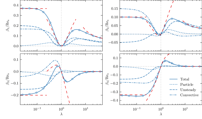
We compute the contributions to from three sources: particle inertia, unsteady fluid inertia and convective fluid inertia. Although the result is only valid for neutrally buoyant particles (), it is interesting to consider the contributions separately:
| (43) |
The contribution from particle inertia is straightforward to compute and can be expressed in closed form as
| (44) |
The coefficients on the r.h.s. of these equations are tabulated for both prolate and oblate spheroids in Table 3 in Appendix A. The coefficients in Eq. (44) are shown as dotted lines in Fig. 2.
| Thin oblate particles () | ||||
|---|---|---|---|---|
| Total | Unsteady | Convective | Particle | |
| Nearly spherical particles () | ||||
| Total | Unsteady | Convective | Particle | |
| Thin prolate particles () | ||||
| Total | Unsteady | Convective | Particle | |
The expressions for the contributions from fluid inertia are very lengthy and not particularly instructive. We therefore present the full result graphically as function of aspect ratio in Fig. 2. In addition we give the asymptotic behavior of all contributions to in Table 2 in three limiting cases: thin oblate particles (), thin prolate particles (, and nearly spherical particles. For nearly spherical particles we define a small parameter as follows
The asymptotic results for , , and for are shown as red dashed lines in Fig. 2.
IV.2 Linear stability analysis at infinitesimal
The effective equations of motion (42) have two special polar angles across which no orbit may pass, regardless of the values of . These angles are (the vorticity direction) and at (the flow-shear plane). In the Jeffery dynamics () the two orbits are called ‘log-rolling’ and ‘tumbling’, and they are both marginally stable, just like all other Jeffery orbits. When the are non-zero but infinitesimal, the log-rolling and tumbling Jeffery orbits still exist for any finite aspect ratio, but their stabilities change.
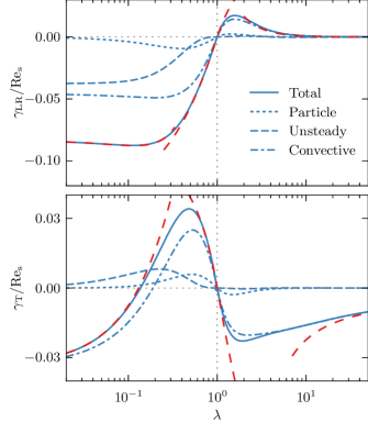
We quantify how particle and fluid inertia lift the degeneracy of the Jeffery orbits by computing the stability exponents for the log-rolling () and tumbling () orbits. The stability exponent is the exponential growth rate over one period of the orbit:
| (45) |
where is the Jeffery period. As we find
| (46) |
For these two exponents are shown as function of particle aspect ratio in Fig. 3. Also shown are their limiting behaviours in the thin oblate limit ()
| (47) | ||||
in the nearly spherical limit ()
| (48) |
and in the thin prolate limit ()
| (49) |
Fig. 3 shows that prolate spheroids of all aspect ratios are unstable at the log-rolling position, and stable at the tumbling orbit. For nearly spherical particles there is a bifurcation: log-rolling and tumbling switch stabilities. For oblate spheroids the log-rolling position is stable for any aspect ratio.
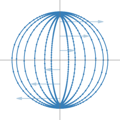
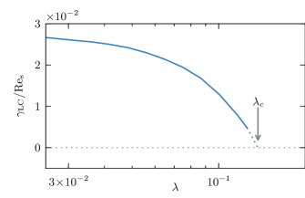
For oblate particles there is a second bifurcation at where the tumbling orbit becomes stable. Clearly, this behavior is caused by the convective inertia of the fluid (see the dash-dotted line in Fig. 3). For sufficiently oblate particles both log-rolling and tumbling orbits are stable, and the long-time dynamics depend on the initial orientation of the particle. Between the two now stable orbits a new unstable limit cycle is born, separating the two basins of attraction.
Fig. 4 shows how the shape of this limit cycle depends upon the particle aspect ratio. Close to the bifurcation the limit cycle lies in the neighbourhood of the tumbling orbit. But as the limit cycle approaches the log-rolling orbit. We have computed the stability exponent of the limit cycle at infinitesimal by numerically integrating Eqs. (42). The result is shown in Fig. 5. We see that , and its magnitude is of the same order as that of .
V Discussion
Effective equation of motion. Eq. (42) is an effective equation of motion for the orientational dynamics of a neutrally buoyant spheroid in a simple shear flow. How the dynamics depends upon the particle aspect ratio is determined by four coefficients . Fig. 2 shows the four functions . Limiting behaviours of the are tabulated in Table 2. We see that the -coefficients tend to zero as , but they approach constants as . In both limits the contribution from particle inertia must tend to zero because the volume of the particle does. The effects of fluid inertia vanish as because the particle effectively disappears in the slender-body limit, the perturbation caused by the particle decreases as as the asymptotic form in Table 2 shows. We remark that the leading-order term in this asymptotic form makes a substantial correction to the slender-body theory for aspect ratios of order .
An oblate particle, on the other hand, always presents no-slip boundaries to the fluid, with an area of the order of as . Therefore the contribution of fluid inertia approaches a constant. We note that the asymptotic forms of the coefficients listed in Table 2 yield accurate values for and , as Fig. 2 shows.
We see in Fig. 2 that the particle-inertia contribution to the coefficients is always much smaller than the fluid-inertia contributions. In general both unsteady and convective fluid inertia contribute, and it would be qualitatively wrong to neglect one of these terms. This is due to the fact that the timescale of the particle motion is the same as the timescale of the flow, and it raises the question under which circumstances both effects may matter for the tumbling of small particles in unsteady flows, and in particular in turbulence.
Linear stability analysis at infinitesimal . The stability exponents of tumbling and log-rolling orbits are shown in Fig. 3. We find that the log-rolling orbit is unstable for prolate spheroids of any aspect ratio, tumbling is stable for prolate spheroids, and no other orbit exist at infinitesimal . For moderately oblate particles with aspect ratios the stabilities are reversed: log-rolling is stable, tumbling is unstable, and no other periodic orbits exist for infinitesimal . At there is a bifurcation where an unstable periodic orbit is born close to the tumbling orbit, which in turn becomes stable. As becomes even smaller, the unstable orbit moves closer to the log-rolling orbit (Fig. 4). We remark that the asymptotic forms (47) and (49) of the stability exponents yield very accurate approximations for the log-rolling exponent, save for aspect ratios close to unity. For the tumbling exponent the asymptotes do not work equally well.
Our results are in agreement with results of recent DNS studiesQi and Luo (2003); Yu, Phan-Thien, and Tanner (2007); Huang et al. (2012); Rosén, Lundell, and Aidun (2014); Mao and Alexeev (2014) determining the orientational dynamics of a neutrally buoyant spheroid in a simple shear flow. These studies are conducted for a number of different aspect ratios with shear Reynolds numbers ranging from moderate to large. At the smallest values of accessible in the DNS no stable log-rolling is found for prolate spheroids of any aspect ratio. For oblate particles with aspect ratio DNS show stable log-rolling and unstable tumbling at the smallest that were simulatedMao and Alexeev (2014), also in agreement with our results. There are no simulations for particles for at small .
SaffmanSaffman (1956) predicted that log-rolling is stable for nearly spherical prolate particles, at variance with the behaviour described above. We do not know why the original calculation fails to give the correct stability of log-rolling. Since no details of the calculation are given it is difficult to figure out the precise origin of this discrepancy. Subramanian & KochSubramanian and Koch (2006) also computed the stability of the log-rolling orbit for nearly spherical particles and came to the same conclusion as Saffman, different from ours. We have compared the small- limit of our calculation to the results of Ref. 17 and find that the particle-inertia correction to the equation of motion agrees, Eqs. (3.15) and (3.16) in Ref. 17. But the fluid-inertia correction does not satisfy the symmetries of the problem. We believe that this explains the discrepancy.
We have independently calculated the stability of log-rolling for nearly spherical particles by expanding the particle-angular velocity jointly in and , using spherical harmonics as a basis setCandelier et al. (2015). The results of this calculation agree to order with the results presented above. Further we have checked that the particle-inertia correction in Eq. (42) is consistent with the results obtained in Ref. 9. We also compared the slender-body limit of our results to the prediction of Subramanian & Koch for the dynamics of slender fibresSubramanian and Koch (2005) and found that the fluid-inertia corrections agree (up to a factor of ).
These observations indicate that the results presented in this paper are correct, explain the results of DNS and resolve the puzzle concerning the stability of log-rolling of spheroids in a simple shear at small .
A new benchmark for DNS at small . Recently a number of groups have developed DNS codes based on the lattice Boltzmann method to simulate the dynamics of particles in flowsQi and Luo (2003); Huang et al. (2012); Rosén, Lundell, and Aidun (2014); Mao and Alexeev (2014). Much effort is spent on validating the model, studying for instance the effects changing grid size, time step, size of the simulation box, and so forth. The benchmark adopted is often the question whether Jeffery orbits are seen for a neutrally buoyant spheroid in a simple shear at small Reynolds numbers. But the limit can never be strictly reached in the simulations. DNS at small values of (specifically: in the linear regime), by contrast, allow precise comparisons with the results obtained in this paper. One could for instance compare trajectories, stability exponents, and period times. We thus expect that our results can serve as benchmarks for present and future DNS codes.
VI Conclusions
In this paper we have derived an effective equation of motion for the orientational dynamics of a neutrally buoyant spheroid suspended in a simple shear flow. The equation is valid for arbitrary aspect ratios and to linear order in , at small but finite shear Reynolds numbers. The effective equation of motion allows us to determine how the degeneracy of the Jeffery orbits is lifted by weak inertial effects. We have determined the bifurcations that occur at infinitesimal as the particle aspect ratio changes. For prolate spheroids log-rolling is unstable, for oblate spheroids it is stable. Tumbling in the shear plane is stable for prolate particles and unstable for nearly spherical oblate particles. For thin disks with aspect ratios , both log-rolling and tumbling are stable. An unstable limit cycle separates the basins of attraction of the periodic orbits.
Our results imply that tumbling and log-rolling orbits survive a finite perturbation whose magnitude depends on the aspect ratio . It would be of interest to derive a bifurcation diagram in the --plane for small . We plan to determine how the small- region of this diagram connects to the intricate bifurcation patterns that were found by Rosén, Lundell & AidunRosén, Lundell, and Aidun (2014) at larger shear Reynolds numbers. We expect that the results summarised here can guide numerical computations with the lattice Boltzmann method that become difficult at small and large aspect ratios.
References
- Jeffery (1922) G. B. Jeffery, “The motion of ellipsoidal particles immersed in a viscous fluid,” Proceedings of the Royal Society of London. Series A 102, 161–179 (1922).
- Subramanian and Koch (2005) G. Subramanian and D. L. Koch, “Inertial effects on fibre motion in simple shear flow,” Journal of Fluid Mechanics 535, 383–414 (2005).
- Qi and Luo (2003) D. Qi and L. Luo, “Rotational and orientational behaviour of three-dimensional spheroidal particles in Couette flows,” J. Fluid Mech. 477, 201 (2003).
- Huang et al. (2012) H. Huang, X. Yang, M. Krafczyk, and X.-Y. Lu, “Rotation of spheroidal particles in Couette flows,” J. Fluid Mech. 692, 369–394 (2012).
- Rosén, Lundell, and Aidun (2014) T. Rosén, F. Lundell, and C. K. Aidun, “Effect of fluid inertia on the dynamics and scaling of neutrally buoyant particles in shear flow,” J. Fluid Mech. 738, 563–590 (2014).
- Mao and Alexeev (2014) W. Mao and W. Alexeev, “Motion of spheroid particles in shear flow with inertia,” J. Fluid Mech. 749, 145 (2014).
- Saffman (1956) P. G. Saffman, “On the motion of small spheroidal particles in a viscous liquid,” J. Fluid Mech. 1, 540 (1956).
- Lundell and Carlsson (2010) F. Lundell and A. Carlsson, “Heavy ellipsoids in creeping shear flow: Transitions of the particle rotation rate and orbit shape,” Physical Review E 81, 016323 (2010).
- Einarsson, Angilella, and Mehlig (2014) J. Einarsson, J. R. Angilella, and B. Mehlig, “Orientational dynamics of weakly inertial axisymmetric particles in steady viscous flows,” Physica D: Nonlinear Phenomena 278–279, 79–85 (2014).
- Kim and Karrila (1991) S. Kim and S. J. Karrila, Microhydrodynamics: principles and selected applications, Butterworth-Heinemann series in chemical engineering (Butterworth-Heinemann, Boston, 1991).
- Einarsson et al. (2015) J. Einarsson, F. Candelier, F. Lundell, J. Angilella, and B. Mehlig, “The effect of weak inertia upon Jeffery orbits,” preprint (2015).
- Harper and Chang (1968) E. Y. Harper and I.-D. Chang, “Maximum dissipation resulting from lift in a slow viscous shear flow,” J. Fluid Mech. 33, 209–225 (1968).
- Saffman (1965) P. G. Saffman, “The lift on a small sphere in a slow shear flow,” J. Fluid Mech. 22, 385–400 (1965).
- Hinch and Leal (1972) E. J. Hinch and L. G. Leal, “The effect of Brownian motion on the rheological properties of a suspension of non-spherical particles,” J. Fluid Mech. 52, 683–712 (1972).
- Petrie (1999) C. J. Petrie, “The rheology of fibre suspensions,” J. Non-Newton. Fluid 87, 369 – 402 (1999).
- Lundell, Soderberg, and Alfredsson (2011) F. Lundell, D. Soderberg, and H. Alfredsson, “Fluid mechanics of papermaking,” Annu. Rev. Fluid Mech. 43, 195–217 (2011).
- Subramanian and Koch (2006) G. Subramanian and D. L. Koch, “Inertial effects on the orientation of nearly spherical particles in simple shear flow,” Journal of Fluid Mechanics 557, 257–296 (2006).
- Yu, Phan-Thien, and Tanner (2007) Z. Yu, N. Phan-Thien, and R. Tanner, “Rotation of a spheroid in a Couette flow at moderate Reynolds numbers,” Phys. Rev. E 76, 026310 (2007).
- Lorentz (1896) H. Lorentz, “The theorem of Poynting concerning the energy in the electromagnetic field and two general propositions concerning the propagation of light,” Versl. Kon. Akad. Wetensch. Amsterdam 4, 176 (1896).
- Happel and Brenner (1983) J. Happel and H. Brenner, Low Reynolds number hydrodynamics (Kluwer Acad. Publisher, 1983).
- Chwang and Wu (1975) A. T. Chwang and T. Y.-T. Wu, “Hydromechanics of low-Reynolds-number flow. Part 2. Singularity method for Stokes flows,” Journal of Fluid Mechanics 67, 787–815 (1975).
- Candelier et al. (2015) F. Candelier, J. Einarsson, F. Lundell, B. Mehlig, and J. Angilella, “The role of inertia for the rotation of a nearly spherical particle in a general linear flow,” preprint (2015).
Appendix A Solutions to Stokes’ equation
In this Appendix we solve the steady Stokes’ equation for an arbitrarily aligned spheroid in a general linear flow . The calculation is a special case of the calculation by Jeffery (1922). However, instead of the ellipsoidal harmonics that Jeffery used, we employ a finite multipole expansion, following Chwang and Wu (1975). The purpose of this Appendix is to derive an explicit closed form expression for the Stokes flow field, suitable for evaluation in the reciprocal theorem. For a more general description of the method we refer to the book by Kim and Karrila (1991).
Formulation of the problem. Stokes’ equation reads:
| (50) |
with no-slip boundary conditions on the surface of the particle
| (51) |
Here is the angular velocity of the particle. Furthermore it is assumed that the flow remains unperturbed at infinitely far away from the particle
| (52) |
We solve for the disturbance flow that satisfies Stokes’ equation (50) with boundary conditions
| (53) |
We decompose the linear background flow into its symmetric and antisymmetric parts, defining the vector and strain by
| (54) |
Finally, in terms of the ‘slip angular velocity’ , the problem to be solved reads
| (55) |
Multipoles. We solve Eq. (55) by a finite multipole expansion Chwang and Wu (1975); Kim and Karrila (1991). The multipoles are the Green’s function for the Stokes’ equation, and its derivatives. In this Appendix we use the shorthand notation . The multipoles needed to solve for the fluid velocity field around particles in a linear flow are
| (56) |
The following two higher-order multipoles are required in the reciprocal theorem. We include them for reference:
| (57) |
Note that we use the “Oseen tensor” notation. The Green’s function for the Stokes’ equation is in fact . It is convenient to split the dipole contribution into its antisymmetric (‘rotlet’) and symmetric (‘stresslet’) parts. They are
| (58) |
Spheroidal multipoles. Whereas the flow around a spherical particle may be represented by multipoles anchored at a single point, representing the flow around a spheroidal particle requires a weighted line distribution of multipoles Chwang and Wu (1975); Kim and Karrila (1991). We therefore define the ‘spheroidal multipoles’ as the following distributions, note especially the different weights for higher-order multipoles:
| (59) |
The constant is related to the spheroidal geometry. Prolate and oblate coordinates are obtained by rotating an ellipse around its major or minor axis. We call the distance between the foci of the underlying ellipse , and then for prolate coordinates, and for oblate coordinates (see definition of coordinate systems in Appendix C.)
In order to write down explicit tensor expressions for the spheroidal multipoles we introduce the integrals , and by
| (60) |
The spatial variation of the functions depends upon and only. Further properties and evaluation of the integrals are discussed in Appendix B. With and we express the spheroidal multipoles explicitly, for example the spheroidal rotlet:
The integrals play the same part in spheroidal geometry as does in spherical geometry. The spheroidal stresslet and quadrupole are given by
| (61) |
| (62) |
Solution by a finite multipole expansion. The spheroidal multipoles are functions that satisfy Stokes’ equation, and a suitable linear combination of them also satisfies the no-slip boundary condition on the surface of a spheroid with symmetry axis . The remaining problem is to determine the coefficients for this linear combination.
Following Kim and Karrila (1991) we use the following ansatz for the disturbance flow field:
| (63) | ||||
where
| (64) |
Given the ambient strain , and angular slip velocity we must determine seven unknown scalars, which may depend upon the particle shape: , , , , , , and . When the coefficients are known, Eq. (63) is the sought Stokes solution.
In order to match the linear boundary condition Eq. (53) we need the combinations of and in the ansatz to be constant on the particle surface, much like the scalar function is in spherical geometry.
Upon examination, the functions and are constant on the spheroidal surface. Further, the functions and can be written as and , where and are constant on the spheroidal surface. The remaining spheroidal functions and which appear in the ansatz (63) are more complicated. However, it turns out that they appear only in the combinations . We therefore choose
| (65) |
With this choice of it holds that, on the surface of the spheroid,
| (66) |
both for prolate and oblate spheroids.
In order to extract the six independent equations for the six remaining coefficients we exploit that the boundary condition must be satisfied for any choice of , and . First, with we contract Eq. (53) with , and . Secondly, with , we contract Eq. (53) with , and finally . These six equations together have only one solution. We tabulate the resulting expressions for both oblate and prolate spheroids in Table 3.
Computing the torque on a body due to this flow is straightforward, because by constructionChwang and Wu (1975) the torque on a body due to the rotlet flow is , where is the rotlet strength. The minus sign is due to the fact that the torque is exerted on body by the flow. To compute the torque from the spheroidal rotlet (59) we linearly superpose the contributions from all the contained rotlets. The torque from the flow is therefore
| (67) |
The factor depends only on the aspect ratio of the particle (see Table 3).
| Expressions common to both prolate and oblate spheroids | ||||||||||||||||||||||||||
|---|---|---|---|---|---|---|---|---|---|---|---|---|---|---|---|---|---|---|---|---|---|---|---|---|---|---|
|
||||||||||||||||||||||||||
Appendix B Spheroidal integrals
In order to solve Stokes’ equation and evaluating the volume integrals in the reciprocal theorem we need to solve integrals on the form
| (68) |
First, when matching boundary conditions we must evaluate the integrals with on the surface of the spheroidal particle. Second, when evaluating the reciprocal theorem we need to integrate products of two or three multiplied with the components of the spatial coordinate over the entire fluid volume outside the particle. Therefore we express the functions in a spheroidal coordinate system with symmetry axis along . This is accomplished by a rotational change of variables , , where the latter equality defines a rotation . The absolute value (distance) between and is preserved by a rotation, and the integral is transformed into
| (69) |
This form is equivalent to the integrals in Chwang and Wu (1975). Geometrically, Eq. (68) represents a line source along the direction . The rotation places the line source along the -axis in an auxiliary coordinate system. The result is a function of and .
Explicit expressions for may be found by direct integration, or by a recursion formulaChwang and Wu (1975). Since we require only a finite number of integrals, we simply perform the direct integration once and for all and save the result in a table.
Finally, when evaluating the term corresponding to unsteady fluid inertia in the volume integral of the reciprocal theorem, we need to compute the derivatives of with respect to the moving vector . By differentiating Eq. (68) we derive the following formula:
| (70) |
Appendix C Spheroidal coordinates
Both oblate and prolate spheroidal coordinates are extensions of a two-dimensional elliptic coordinate system (). The -coordinate represents concentric ellipses, while represents the corresponding hyperbolas. Their intersections give unique coordinates in the --plane. An azimuthal angle of revolution denotes the extension into three dimensions.
Oblate spheroidal coordinates. Start with the --plane, and place an ellipse of focal distance with its minor axis along the -axis. Now revolve the ellipse by around the -axis to produce an oblate spheroid. Then represents concentric oblate spheroidal surfaces, represents the corresponding hyperbolic surfaces, and we call the angle of revolution. The coordinate equations are
| (71) |
The coordinate ranges are , and , and the volume element .
In this paper we treat oblate spheroids with dimensionless major axis length unity, and minor axis length . These lengths determine the focal distance as
| (72) |
and the particle surface is parameterised by
| (73) |
Prolate spheroidal coordinates. Start with the --plane, and place an ellipse of focal distance with its major axis along the -axis. Now revolve the ellipse by around the -axis to produce a prolate spheroid. Then represents concentric prolate spheroidal surfaces, represents the corresponding hyperbolic surfaces, and we call the angle of revolution. The coordinate equations are
| (74) |
The coordinate ranges are , and , and the volume element .
In this paper we treat prolate spheroids with dimensionless major axis length unity, and minor axis length . These lengths determine the focal distance as
| (75) |
and the particle surface is parameterised by
| (76) |