Optimal induced universal graphs and adjacency labeling for trees

Abstract

We show that there exists a graph $G$ with $O(n)$ nodes, such that any forest of $n$ nodes is a node-induced subgraph of $G$. Furthermore, for constant arboricity $k$, the result implies the existence of a graph with $O(n^{k})$ nodes that contains all $n$-node graphs of arboricity $k$ as node-induced subgraphs, matching a $\Omega(n^{k})$ lower bound. The lower bound and previously best upper bounds were presented in Alstrup and Rauhe [FOCS’02]. Our upper bounds are obtained through a $\log_{2}n+O(1)$ labeling scheme for adjacency queries in forests.

We hereby solve an open problem being raised repeatedly over decades, e.g. in Kannan, Naor, Rudich [STOC’88], Chung [J. of Graph Theory’90], Fraigniaud and Korman [SODA’10].

1 Introduction

An adjacency labeling scheme for a given family of graphs assigns labels to the vertices of each graph from the family such that given the labels of two vertices from a graph, and no other information, it is possible to determine whether or not the vertices are adjacent in the graph. The labels are assumed to be bit strings, and the goal is to minimize the maximum label size. A $k$-bit labeling scheme (sometimes denoted $k$ labeling scheme) uses at most $k$ bits per label. In information theory adjacency labeling schemes studies goes back to the 1960’s [22, 23], and efficient labeling schemes were introduced in [57, 69]. Adjacency labeling schemes are also called implicit representation of graphs [83, 90].

As an example let $\mathcal{A}_{n}$ denote the family of forests with $n$ nodes. Given a forest $F\in\mathcal{A}_{n}$, do the following: Root the trees of $F$ and assign each node with an id from $[0,n-1]$. Let the label of each node be its id appended with the id of its parent. A test for adjacency is then simply to test whether the id of one of the nodes equals the stored parent id of the other node. The labels assigned to the nodes have length $2\lceil\log n\rceil$ bits.

Closely related to adjacency labeling schemes are induced-universal graphs also studied in the 1960’s [67, 79]. A graph $G=(V,E)$ is said to be an induced-universal graph for a family $\cal F$ of graphs, if it contains all graphs in $\cal F$, as node-induced subgraphs. A graph $H=(V^{\prime},E^{\prime})$ is contained in $G$ as a node-induced subgraph if $V^{\prime}\subseteq V$ and $E^{\prime}=\{(v,w)|v,w\in V^{\prime}\wedge(v,w)\in E\}$. We define $g_{v}(\mathcal{F})$ to be the smallest number of nodes in any induced-universal graph for $\mathcal{F}$. From [57] (some details given in [11, 83]) we have:

Theorem 1 ([57]).

A family, $\mathcal{F}$, of graphs has a $k$-bit adjacency labeling scheme with unique labels iff $g_{v}(\mathcal{F})\leq 2^{k}$.

Labels being unique means that no two nodes in the same graph from $\mathcal{F}$ will be given the same label.

Combining the $2\lceil\log n\rceil$-bit labeling scheme above with Theorem 1 gives $g_{v}(\mathcal{A}_{n})=O(n^{2})$. Closely related, a universal graph for ${\cal F}$ is a graph that contains each graph from ${\cal F}$ as a subgraph, not necessarily induced. The challenge is to construct universal graphs with as few edges as possible. Let $f_{e}(\mathcal{F})$ denote the minimum number of edges in a universal graph for $\mathcal{F}$. In a series of papers [12, 27, 28, 29, 30, 32, 72] it was established that $f_{e}(\mathcal{A}_{n})=\Theta(n\log n)$. Let $G=(V,E)$ be any universal graph for any family $\mathcal{H}$ of acyclic graphs. In [27] Chung shows $g_{v}(\mathcal{H})\leq 2|E|+|V|$ and, combined with bounds for $f_{e}(\mathcal{A}_{n})$, concludes that $g_{v}(\mathcal{A}_{n})=O(n\log n)$. As the bounds for $f_{e}(\mathcal{A}_{n})$ are tight it is not possible to improve the bounds for $g_{v}(\mathcal{A}_{n})$ using the techniques of [27]. However, for the family of graphs of forests with bounded degree and $n$ nodes, denoted $\mathcal{A}^{B}_{n}$, there exists a universal graph with $n$ nodes and $O(n)$ edges [15, 16], giving $g_{v}(\mathcal{A}^{B}_{n})=O(n)$ [27].

Chung’s results [27] combined with Theorem 1 give a $\log n+\log\log n+O(1)$ adjacency labeling scheme for forests, and $\log n+O(1)$ for bounded degree forests. In 2002 Alstrup and Rauhe [11] gave a $\log n+O(\log^{*}n)$ adjacency labeling scheme for general forests. Adjacency labeling schemes using $\log n+O(1)$ bits are given in [19, 20, 21] for bounded degree forests and caterpillars, in [45] for bounded depth trees, and in [44] the case allowing 1-sided errors. Adjacency labeling schemes for forests are also considered in [3, 58]. Table 1 summarizes the results.

Graph family	Upper bound	Reference
Forests of bounded degree	$O(n)$	[27]
Forests	$n2^{O(\log^{*}n)}$	[11]
Caterpillars	$O(n)$	[19]
Trees of depth $d$	$O(nd^{3})$	[45]
Forests	$O(n)$	This paper

Table 1: Size of induced-universal graphs for various families of forests.

While minimizing the label size is the main goal of a labeling scheme, we sometimes also seek to reduce the running time. The time used to assign labels to the nodes is called the encoding time, and the time used to decide whether two nodes are adjacent or not is called the decoding time. In [19, 20, 21] described above the encoding time is $O(n)$ and decoding time is $O(1)$.

Addressing a problem repeatedly raised the last decades, e.g. in [3, 19, 27, 28, 29, 44, 45, 49, 57] we show:

Theorem 2.

There exists an adjacency labeling scheme for $\mathcal{A}_{n}$ using unique labels of length $\log n+O(1)$ bits with $O(1)$ decoding time and $O(n)$ encoding time in the word-RAM model.

In our solution the decoder does not know $n$ in advance. The importance of the problem is emphasized by it repeatedly and explicitly being raised as a central open problem (see appendix A). Theorem 2 establishes that adjacency labeling in forests requires $\log n+\Theta(1)$ bits. To see this, consider the path of length $n$ as well as the star on $n$ nodes. These two graphs may share at most $n/2$ labels, giving a $\log 1.5n=\log n+\Omega(1)$ lower bounds. We note that this lower bound may be slightly improved using the result of [73].

1.1 Graphs with bounded arboricity

Let $\mathcal{F}$ and $\mathcal{Q}$ be two families of graphs and let $G$ be an induced-universal graph for $\mathcal{F}$. Suppose that every graph in the family $\mathcal{Q}$ can be edge-partitioned into $k$ parts, each of which forms a graph in $\mathcal{F}$. In this case, it was shown by Chung [27] that $g_{v}(\mathcal{Q})\leq|V(G)|^{k}$. She considered the family, $\mathcal{A}_{n}^{k}$ of graphs with arboricity $k$ and $n$ nodes. A graph has arboricity $k$ if the edges of the graph can be partitioned into at most $k$ forests. By combining the above result with $g_{v}(\mathcal{A}_{n})=O(n\log n)$ she showed that $g_{v}(\mathcal{A}_{n}^{k})=O((n\log n)^{k})$ improving the bound of $n^{k+1}$ from [57]. For constant arboricity $k$, it follows from [11] that $\Omega(n^{k})=g_{v}(\mathcal{A}_{n})\leq n^{k}2^{O(\log^{*}n)}$. Combining Chung’s reduction [27] with Theorem 1 and 2 we show that:

Theorem 3.

There exists an induced-universal graph of size $O(n^{k})$ for the family of graphs with constant arboricity $k$ and $n$ nodes.

Achieving results for bounded degree graphs by reduction to bounded arboricity graphs is e.g. used in [57]. This can be done as graphs with bounded degree $d$ have arboricity bounded by $\left\lfloor{\frac{d}{2}}\right\rfloor+1$ [25, 64].

1.2 Adjacency labeling and induced-universal graphs for other families

Induced-universal graphs (and hence adjacency labeling schemes) are given for tournaments [14, 68], hereditary graphs [65, 81], threshold graphs [56], special commutator graphs [78], bipartite graphs [66], bounded degree graphs [85], and other cases [17, 74]. Using universal graphs constructed by Babai et al. [12], Bhatt et al. [16] and Chung et al. [28, 29, 30, 32], Chung [27] obtains the current best bounds for e.g. induced-universal graphs for bounded degree graphs being planar or outerplanar. Many other results use reductions from [27], e.g. the induced-universal graphs for bounded degree graphs [24, 39]. The result from  [39], as many others, is achieved by reduction to a universal graph with bounded degree [4, 5]. Other results for universal graphs is e.g. for families of graphs such as cycles [18], forests [31, 42], bounded degree forests [15, 47], and graphs with bounded path-width [84]. In [9] they give a $(\left\lceil{n/2}\right\rceil+4)$-bit adjacency labeling scheme for general undirected graphs, improving the $(\lfloor n/2\rfloor+\lceil\log n\rceil)$ bound of [67], almost matching an $(n-1)/2$ lower bound [57, 67]. An overview of induced-universal graphs and adjacency labeling can be found in [9].

1.3 Second order terms for labeling schemes are theoretically significant

Above it is shown that for adjacency labeling significant work has been done optimizing the second order term. This is also true for other labeling scheme operations. E.g. the second order term in the ancestor relationship is improved in a sequence of STOC/SODA papers [2, 6, 10, 45, 46] (and [1, 59]) to $\Theta(\log\log n)$, giving labels of size $\log n+\Theta(\log\log n)$. Lastly, an algorithm giving both a simple and optimal scheme was given in [35]. Somewhat related, succinct data structures (see, e.g., [36, 40, 41, 70, 71, 75]) focus on the space used in addition to the information theoretic lower bound, which is often a lower order term with respect to the overall space used.

1.4 Labeling schemes in various settings and applications

By using labeling schemes, it is possible to avoid costly access to large global tables, computing instead locally and distributed. Such properties are used in applications such as XML search engines [2], network routing and distributed algorithms [34, 37, 43, 89], dynamic and parallel settings  [33, 62], and various other applications [61, 76, 80].

Various computability requirements are sometimes imposed on labeling schemes [2, 57, 60]. This paper assumes the RAM model and mentions the time needed for encoding and decoding in addition to the label size.

Closely related to adjacency is small distances in trees. This is studied by Alstrup et al. in [7] who among other things give a $\log n+\Theta(\log\log n)$ labeling scheme supporting both parent and sibling queries. General distance labeling schemes for various families of graphs exist, e.g., for trees [7, 77], bounded tree-width, planar and bounded degree graphs [52], some non-positively curved plane [26], interval [50] and permutation graphs [13], and general graphs [53, 91]. In [52] it is proved that distance labels require $\Theta(\log^{2}n)$ bits for trees. Approximate distance labeling schemes are also well studied; see e.g., [54, 55, 63, 86, 87, 88]. An overview of distance labeling schemes can be found in [8], and a more general labeling survey can be found in an overview in [51].

2 Preliminaries

In this section we introduce some well-known results and notation. Throughout this paper we use the convention that $\lg x=\max(1,\log_{2}x)$ for convenience. We assume the word-RAM model of computation.

Trees

Let $\mathcal{T}_{n}$ denote the family of all rooted trees of size $n$ and let $T\in\mathcal{T}_{n}$. We denote the nodes of $T$ by $V(T)$ and the edges by $E(T)$. We let $\left|T\right|$ denote the number of nodes in $T$. For a node $u\in V(T)$, we let $T_{u}$ denote the subtree of $T$ rooted in $u$. A node $u$ is an ancestor of a node $v$ iff it is on the unique path from $v$ to the root. In this case we also say that $v$ is a descendant of $u$. A caterpillar is a tree whose non-leaf nodes induce a path. Throughout the paper we will only consider adjacency labeling in trees, as we may add an ‘‘imaginary root’’ to any forest on $n$ nodes turning it into a tree of size $n+1$. To do this we expend at most one extra bit to distinguish this from actual nodes.

Heavy-light

For a node $u$ with children $children(u)=v_{1},\ldots,v_{k}$, with $|T_{v_{k}}|\geq|T_{v_{i}}|$ for all $i<k$, we say that the edge $(u,v_{k})$ is heavy, and the remaining edges $(u,v_{i})$ are light. We say that $heavy(u)=v_{k}$ is the heavy child of $u$. A node $u$ for which the edge $(parent(u),u)$ is light is called an apex node. For convenience we also define the root to be an apex node. For a node $u$, we define $children(u)\,\setminus\,\{heavy(u)\}$ to be the light children of $u$. This is called a heavy-light decomposition [82] as it decomposes the tree into paths of heavy edges (heavy paths) connected by light edges. We define the light subtree of a node $u$ to be $T_{u}^{\ell}=T_{u}\setminus T_{heavy(u)}$. For a leaf $u$, $T_{u}^{\ell}=T_{u}=u$. The light depth of a node $u$ is the number of light edges on the path from $u$ to the root. The light height of a node $u$ is the maximum number of light edges on a path from $u$ to a leaf in $T_{u}$.

Lemma 1.

[82] Given a tree $T$ and $u\in V(T)$ with light height $x$, $|T_{u}|\geq 2^{x+1}-1$.

Bit strings

A bit string $s$ is a member of the set $\{0,1\}^{*}$. We denote the length of a bit string $s$ by $|s|$, the $i$th bit of $s$ by $s_{i}$, and the concatenation of two bit strings $s,s^{\prime}$ by $s\circ s^{\prime}$ (i.e. $s=s_{1}\circ s_{2}\circ\ldots\circ s_{|s|}$). We say that $s_{1}$ is the most significant bit of $s$ and $s_{|s|}$ is the least significant bit. For an integer $x$ we let $0^{x}$ and $1^{x}$ denote the strings consisting of exactly $x$ $0$s and $1$s respectively. Let $a$ be an integer and let $s$ be the bit string representation of $a$. Define the function $wlsb(a,k)$ to be $s_{1}\circ s_{2}\circ\cdots\circ s_{|s|-k}$, i.e. the bit string of $a$ without the $k$ least significant bits. When $k>|s|$ we define $wlsb(a,k)$ to be the empty string. When constructing a labeling scheme we often wish to concatenate several bit strings of unknown length. We may do this using the Elias $\gamma$ code [38] to encode a length $k$ bit string with $2k$ bits and decode it in $O(1)$ time for $k=O(w)$, using standard bit operations.

For an integer $a$ we will often use $a$ to denote the bit string representation of $a$ when it is clear from the context. We will use $[a]_{\gamma}$ to denote the Elias $\gamma$ encoding of $a$.

Labeling schemes

An adjacency labeling scheme for trees of size $n$ consists of an encoder, $e$, and a decoder, $d$. Given a tree $T\in\mathcal{T}_{n}$, the encoder computes a mapping $e_{T}:V(T)\to\left\{0,1\right\}^{*}$ assigning a label to each node $u\in V(T)$. The decoder is a mapping $d:\left\{0,1\right\}^{*}\times\left\{0,1\right\}^{*}\to\{{\tt True},{\tt False}\}$ such that given any tree $T\in\mathcal{T}_{n}$ and any pair of nodes $u,v\in V(T)$ we have $d(e_{T}(u),e_{T}(v))={\tt True}$ iff $(u,v)\in E(T)$. Note that the decoder does not know $T$. The size of a labeling scheme is defined as the maximum label size $|e_{T}(u)|$ over all trees $T\in\mathcal{T}_{n}$ and all nodes $u\in V(T)$. If for all trees $T\in\mathcal{T}_{n}$ the mapping $e_{T}$ is injective we say that the labeling scheme assigns unique labels. The labeling schemes constructed in this paper all assign unique labels and the decoder does not know $n$.

Approximation

Given a non-negative integer $a$ and a real number $\varepsilon>0$, a $(1+\varepsilon)$-approximation of $a$ is an integer $b$ such that $a\leq b<(1+\varepsilon)a$. We also define $b=0$ to be the unique $(1+\varepsilon)$-approximation of $a=0$.

Lemma 2.

Given an integer $a$ and a number $\varepsilon\in(0,1]$, we can find a $(1+\varepsilon)$-approximation and represent it using $O(\lg\lg a+\lg\frac{1}{\varepsilon})$ bits. Furthermore, if $\varepsilon=\frac{1}{\delta}$, where $\delta$ is a positive integer that can be stored using $O(1)$ words, we can find this approximation in $O(1)$ time.

Proof.

We will use a single bit to distinguish between the cases $a=0$ and $a>0$, so assume $a>0$. Let $\delta=\left\lceil{\varepsilon^{-1}}\right\rceil$ and $\varepsilon^{\prime}=\delta^{-1}$. Let $k=\left\lceil{\log_{1+\varepsilon^{\prime}}a}\right\rceil$. Then $(1+\varepsilon^{\prime})^{k}\geq a>(1+\varepsilon^{\prime})^{k-1}$. Hence if we let $b=(1+\varepsilon^{\prime})^{k}$ we have $a\leq b<a(1+\varepsilon^{\prime})\leq a(1+\varepsilon)$. In order to encode $b$ it suffices to encode $\delta$ and $k$. We can do this using $2\left\lceil{\lg\delta}\right\rceil+2\left\lceil{\lg k}\right\rceil$ bits using the Elias $\gamma$ coding. Note that:

$$k-1<\log_{1+\varepsilon^{\prime}}a=\frac{\log_{2}a}{\log_{2}(1+\varepsilon^{\prime})}$$

Taking $\log_{2}$ gives:

$$\log_{2}(k-1) <\log_{2}\log_{2}a-\log_{2}\log_{2}(1+\varepsilon^{\prime})$$

$$=\log_{2}\log_{2}a+O\left(1+\log_{2}\frac{1}{\varepsilon^{\prime}}\right)$$

$$=\log_{2}\log_{2}a+O\left(1+\log_{2}\frac{1}{\varepsilon}\right)$$

Hence $\lg k=O\left(\lg\lg a+\lg\frac{1}{\varepsilon}\right)$, and since $\lg\delta\leq 1+\lg\frac{1}{\varepsilon}$ the proof is finished. ∎

We will use $\textnormal{{Approx}}(a,\varepsilon)$ to denote a function returning a $(1+\varepsilon)$-approximation of $a$ as described above.

3 A simple scheme for caterpillars

As a warmup, we describe a simple adjacency labeling scheme of size $\lg n+O(1)$ for caterpillars. The idea is to use a variant of this scheme recursively when labeling general trees. The scheme we present uses ideas similar to that of [19].

Let $p=(u_{1},\ldots,u_{|p|})$ be a longest path of the caterpillar and root the tree in $u_{1}$. We assign an id and an interval $I(u_{i})=[id(u_{i}),id(u_{i})+l(u_{i}))$ to each node $u_{i}$, such that $id(v)\in I(u_{i})$ iff $v$ is a non-root apex node (all leaves except $u_{|p|}$ are apex nodes) and $u_{i}$ is the parent of $v$. The ids of the $u_{i}$s are assigned such that given the label of $u_{i}$ we can deduce $id(u_{i+1})$ for $i<|p|$. We first calculate the interval sizes $l$ and next assign the $id$s. Both steps can be done in $O(n)$ time.

Interval sizes

Let $\gamma_{i}=\left\lceil{\lg|T_{u_{i}}^{\ell}|}\right\rceil$. For each node $u_{j}$ now define the $|p|$-dimensional vector $\beta_{j}$ as $\beta_{j}(i)=\gamma_{j}-|i-j|$. Let $k_{i}=\max_{j=1\ldots|p|}\beta_{j}(i)$. This ensures that $(k_{i}-k_{i+1})\in\{-1,0,1\}$ for all $i\in\{1,\ldots,|p|-1\}$. The process is illustrated in Figure 1. The interval size of node $u_{i}$ is now set to $l(u_{i})=2^{k_{i}}$.

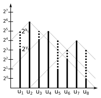
Figure 1: Example of how the $\beta_{j}$s are used to ensure that neighbouring nodes have $(k_{i}-k_{i+1})\in\{-1,0,1\}$.

Id assignment

The idea is to assign $id(u_{i})$ such that the $k_{i}$ least significant bits of $id(u_{i})$ are all $0$. We first assign the id for $u_{1}$ and its children, then $u_{2}$ and its children, etc. The procedure is as follows:

1. Assign $id(u_{i})=x$, where $x$ is the smallest integer having $0$ as the $k_{i}$ least significant bits satisfying $x\geq id(u_{i-1})+l(u_{i-1})$. For $u_{1}$ we set $id(u_{1})=0$.

2. Let $v_{1},\ldots,v_{|T_{u_{i}}^{\ell}|-1}$ be the light children of $u_{i}$. Assign $id(v_{j})=id(u_{i})+j$. Note that $id(v_{|T_{u_{i}}^{\ell}|-1})<id(u_{i})+l(u_{i})$.

The label

For a node $u_{i}\in p$ we assign the label

$$\ell(u_{i})=type(u_{i})\circ[k_{i}]_{\gamma}\circ wlsb(id(u_{i}),k_{i})\ ,$$

and for $v\notin p$, assign the label

$$\ell(v)=type(v)\circ id(v)\ .$$

Here $type(u)$ is $1$ if $u\notin p$. Otherwise, $type(u_{i})$ is $0xx$, where $xx$ is either $00$, $01$, $10$ or $11$ corresponding to the following four cases: (00) $u_{i}=u_{|p|}$, (01) $k_{i}=k_{i+1}-1$, (10) $k_{i}=k_{i+1}$, and (11) $k_{i}=k_{i+1}+1$.

Label size

First, we let $N$ denote the maximum $id$ assigned by the encoder. Then the label size for a node $u_{i}\in p$ is $\leq 3+2\left\lceil{\lg k_{i}}\right\rceil+\left\lceil{\lg N}\right\rceil-k_{i}$ and for $v\notin p$, it is $\leq 1+\left\lceil{\lg N}\right\rceil$. We will now bound $N$:

Lemma 3.

Given a caterpillar $T$ with $n$ nodes, the maximum id assigned by our encoder, $N$, satisfies

$$N\leq 12n\ .$$

Proof.

First, observe that the number of ids skipped between $id(u_{i-1})+l(u_{i-1})$ and $id(u_{i})$ is at most $2^{k_{i}}-1$ as any set of $2^{k_{i}}$ consecutive integers must contain at least one integer with $k_{i}$ $0s$ as least significant bits. Thus, the maximum id is bounded by $\sum_{i=1}^{|p|}\left(2^{k_{i}}-1+l(u_{i})\right)=2\cdot\left(\sum_{i=1}^{|p|}2^{k_{i}}\right)-|p|$ and we can bound this using

$$\left(\sum_{i=1}^{|p|}2^{k_{i}}\right)\leq\left(\sum_{i=1}^{|p|}\sum_{j=1}^{|p|}2^{\beta_{j}(i)}\right)=\left(\sum_{j=1}^{|p|}\sum_{i=1}^{|p|}2^{\beta_{j}(i)}\right)\leq\left(\sum_{j=1}^{|p|}\sum_{i=-\infty}^{\infty}2^{\gamma_{j}-|i|}\right)=\left(\sum_{j=1}^{|p|}3\cdot 2^{\gamma_{j}}\right)$$

concluding that $N\leq 12n-|p|$ ∎

Decoding

Given the labels of $u,v\notin p$ we always answer False.

Now assume that we are given the label of at least one node $u_{i}\in p$. First we deduce $id(u_{i})$ using $[k_{i}]_{\gamma}$ and $wlsb(id(u_{i}),k_{i})$. This also gives us $l(u_{i})=2^{k_{i}}$. Now there are two cases:

1. If the other label is for a node $v\notin p$, we simply read $id(v)$ and answer True if $id(v)\in[id(u_{i}),id(u_{i})+l(u_{i}))$. Otherwise we answer False.

2. If the other label is for $u_{j}\in p$, assume without loss of generality that $id(u_{j})>id(u_{i})$. If $type(u_{i})=001$, set $x$ to be the smallest integer with the $k_{i}+1$ least significantly bits set to $0$ satisfying $x\geq id(u_{i})+l(u_{i})$. If $x=id(u_{j})$ answer True, otherwise answer False.

   The other types can be handled similarly.

4 An optimal scheme for general trees

In this section we prove Theorem 2. Similar to the caterpillar scheme presented in the previous section we assign an id, $id(u)$, and interval, $I(u)$, to each node. The interval and id of a node is assigned such that $id(v)\in I(u)$ iff $v\in T_{u}^{\ell}$. The label of a node $u$ will be assigned such that we can infer the following information (loosely speaking) directly from the label:

• The id of the node $u$.

• The id of $u$’s heavy child, $heavy(u)$.

• The interval $I(u)$ containing the ids of all nodes in $u$’s light subtree.

• Auxilliary information to help decide whether $u$ is a light child of another node.

In order to store this information as part of the label, each node will be assigned an id with a number of trailing zero bits proportional to the logarithm of its interval size corresponding to the $k_{i}$s of Section 3. Furthermore, we ensure that the interval size for a node $u$ is proportional to $|T_{u}^{\ell}|$ (or simply $|T_{u}|$ for apex nodes), and call this the light weight of $u$ denoted by $lw(u)$. Intuitively this ensures that nodes with large subtrees have more ‘‘bits to spare’’.

The labels are assigned using a similar two-step procedure as in Section 3. In the first step we assign the light weight of each node using a recursive procedure, and in the second step we assign the actual ids of the nodes based on the given weights. Both steps are handled in $O(n)$ time. In order to bound the maximum id assigned we introduce the notion of path weights (to be defined later). The path weight of a heavy path $p$ is denoted $pw(u)$, where $u$ is the apex node of $p$.

4.1 Weight classes and restricted light depth

The auxilliary information mentioned above is primarily used to determine adjacency between an apex node and its parent. A classic way of doing this is to use the light depth of both nodes and check that it differs by exactly one. However, the light depth of a node with a small subtree could potentially be big in comparison, and thus we cannot afford to store it. To deal with this we introduce the following notion of weight classes and restricted light depth:

Definition 1.

Let $T$ be a rooted tree and $u$ some node in $T$. Define

$$\gamma(u)=\begin{cases}\left\lfloor{\lg|T_{u}|}\right\rfloor&\text{if $u$ is an apex node}\\ \left\lfloor{\lg|T_{u}^{\ell}|}\right\rfloor&\text{otherwise.}\end{cases}$$ (1)

The weight class of $u$ is defined as $wc(u)=\left\lfloor{\lg\gamma(u)}\right\rfloor$.

Definition 2.

Let $T$ be a rooted tree and $u$ some node in $T$. Define $wtop(u)$ to be the ancestor of $u$ with smallest depth such that every node on the path from $u$ to $wtop(u)$ has weight class $\leq wc(u)$. The restricted light depth of $u$ is the number of light edges on the path from $u$ to $wtop(u)$ and is denoted by $rld(u)$.

An illustration of these definitions can be seen in Figure 2.

Figure 2: Example of weight classes and restricted light depths in a tree. The dotted and solid lines correspond to light and heavy edges respectively.

When assigning the interval $I(u)$, we will split it into a sub-interval for each weight class $i\leq wc(u)$.

We will now show some properties related to weight classes and restricted light depth. We will use the definitions of $\gamma(u)$ and $wtop(u)$ as described in Definitions 1 and 2.

Lemma 4.

Let $u$ be any node, then $rld(u)\leq 2\gamma(u)+1$.

Proof.

Let $v$ be the apex node on the path from $v$ to $wtop(u)$ with the smallest depth. (If no such node exist $rld(u)=0$ and the result is trivial.) We note that $v$ must have light height $\geq rld(u)-1$, so by Lemma 1 $\left|T_{v}\right|\geq 2^{rld(u)}-1$ and therefore $\gamma(v)\geq rld(u)-1$. So

$$2\gamma(u)\geq 2^{wc(u)+1}\geq 2^{wc(v)+1}\geq\gamma(v)\geq rld(u)-1$$

which finishes the proof. ∎

Lemma 5.

Let $u$ be an ancestor of $v$ such that $u$ is an apex node and $wc(u)=wc(v)$. Let $k$ be the number of light edges on the path from $u$ to $v$. Then $rld(v)=rld(u)+k$.

Proof.

Any node in $u$’s subtree must have weight class $\leq wc(u)$ since $u$ is an apex node. Since $wc(u)=wc(v)$ every node on the path from $v$ to $wtop(u)$ must have weight class $\leq wc(v)$. Thus $wtop(v)=wtop(u)$ and there are $rld(u)+k$ light edges on the path from $v$ to $wtop(u)$, i.e. $rld(v)=rld(u)+k$. ∎

Lemma 6.

Let $u$ be the parent of an apex node $v$. If $wc(v)<wc(u)$ then $rld(v)=0$, and if $wc(v)=wc(u)$ then $rld(v)=rld(u)+1$.

Proof.

If $wc(v)<wc(u)$ then $v$ has restricted light depth $0$ so assume that $wc(u)=wc(v)$. Let $w$ be the apex node on $u$’s heavy path (possibly $u$ itself). Then first assume that $wc(w)=wc(u)$. By Lemma 5 $rld(u)=rld(w)$ and $rld(v)=rld(w)+1$ and the claim is true. Now assume that $wc(w)>wc(u)$. Then $rld(u)=0$ and $rld(v)=1$ and the claim is true as well. Since $wc(w)<wc(u)$ is impossible the proof is finished. ∎

4.2 Weight assignment

We will now see how to assign path weights and light weights to the nodes. The idea is to consider an entire heavy path as a ‘‘recursive caterpillar’’ and use ideas similar to those of Section 3. Consider any heavy path $p=(u_{1},u_{2},\ldots,u_{\left|p\right|})$ in order where $u_{1}$ is the apex node. For each $u\in p$ we do the following:

1. For each light-child $v$ of $u$ we recursively calculate $pw(v)$.

2. For every weight class $i\leq wc(u)$, let $b_{i}$ be the sum of $pw(v)$ for all light children $v$ of $u$ with weight class $wc(v)=i$.

3. We use the convention that $a_{0}(u)=0$, and for $i=1,\ldots,wc(u)$ we let $a_{i}(u)$ be a $\left(1+\frac{1}{(\gamma(u))^{3}}\right)$-approximation of $a_{i-1}(u)+b_{i}(u)$.

4. We then define the light weight of $u$ as $lw(u)=1+a_{wc(u)}(u)$.

For each $i=1,2,\ldots,\left|p\right|$ we let $k^{\prime}(u_{i})=\gamma(u_{i})-\left\lceil{2\lg\gamma(u_{i})}\right\rceil+1$. We choose $k(u_{1}),\ldots,k(u_{\left|p\right|})$ such that $k(u_{i})\geq k^{\prime}(u_{i})$ for every $i=1,\ldots,\left|p\right|$ and $k(u_{i})-k(u_{i+1})\in\left\{-1,0,1\right\}$ for all $i=1,\ldots,\left|p\right|-1$. We do this in the same manner as in Section 3 when we constructed the labeling scheme for the caterpillar, see Figure 1.

The path weight of $u_{1}$ is defined as $pw(u_{1})=\sum_{i=1}^{\left|p\right|}\left(lw(u_{i})+2^{k(u_{i})}-1\right)$. By this definition, the path weight of a leaf apex node is $1$.

Pseudocode for the function Assign-Weight is available in Algorithm 1.

input : Heavy path $p=(u_{1},\ldots,u_{t})$ represented by $u_{1}$.

output : path weight of $p$.

1 for $i=1\to t$ do

2       $a_{0}(u_{i})\leftarrow 0$

3       for $j=1\to wc(u_{i})$ do

4             $b_{j}\leftarrow 0$

5             for $v\in\{w\in\textnormal{{Light-Children}}(u_{i})\mid wc(w)=j\}$ sorted by subtree size do

6                   $b_{j}\leftarrow b_{j}+\textnormal{{Assign-Weight}}(v)$

7                  

8             end for

9            $a_{j}(u_{i})=\textnormal{{Approx}}(a_{j-1}(u_{i})+b_{j},\gamma(u_{i})^{-3})$

10            

11       end for

12      $lw(u_{i})=1+a_{wc(u_{i})}(u_{i})$

13      

14 end for

15$k(u_{1})=\gamma(u_{1})-\left\lceil{2\lg\gamma(u_{1})}\right\rceil+1$

16 for $i=2\to t$ do

17       $k(u_{i})=\max(\gamma(u_{i})-\left\lceil{2\lg\gamma(u_{i})}\right\rceil+1,k(u_{i-1})-1)$

18      

19 end for

20for $i=t-1\to 1$ do

21       $k(u_{i})=\max(k(u_{i}),k(u_{i+1})-1)$

22      

23 end for

24$pw(u_{1})\leftarrow 0$

25 for $i=1\to t$ do

26       $pw(u_{1})\leftarrow pw(u_{1})+lw(u_{i})+2^{k(u_{i})}-1$

27      

28 end for

29return $pw(u_{1})$

Algorithm 1 Assign-Weight

The main technical part of this paper is to show that calling Assign-Weight ensures that $pw(u)=O(|T_{u}|)$ for all apex nodes, $u\in T$. This is used to show that the maximum id assigned by our labeling scheme is $O(n)$ and thus takes $\lg n+O(1)$ bits to store. Intuitively this is the case since the quality of the approximation used in a node $u$ improves as the size of $u$’s subtree increases. Specifically, we will use the following lemma, which is proved in Section 5.

Lemma 7.

Let $T$ be a tree rooted in $r$ and let $u\in T$ be any apex node with light height $x$. After calling $\textnormal{{Assign-Weight}}(r)$ it holds that:

$$pw(u)\leq 3\left|T_{u}\right|\cdot\prod_{i=1}^{x}\left(1+\frac{6}{i^{2}}\right)$$

Furthermore, for any node $v\in T$ it holds that

$$lw(v)\leq 3\left|T^{\ell}_{v}\right|\prod_{j=1}^{z}\left(1+\frac{6}{j^{2}}\right)\cdot\left(1+\frac{2}{(z+1)^{2}}\right)\ ,$$ (2)

where $z$ is the maximum light height of any light child of $v$.

Corollary 1.

Let $T$ be a tree rooted in $r$ and let $u\in T$ be any apex node and $v\in T$ be any node. After calling $\textnormal{{Assign-Weight}}(r)$ it holds that:

$$pw(u)\leq 3e^{\pi^{2}}\left|T_{u}\right|,\quad lw(v)\leq 3e^{\pi^{2}}\left|T_{v}^{\ell}\right|$$

Proof.

Let $u$ be an apex node with light height $x$. Then:

$$pw(u) \leq 3\left|T_{u}\right|\cdot\prod_{i=1}^{x}\left(1+\frac{6}{i^{2}}\right)$$

$$\leq 3\left|T_{u}\right|\cdot\exp\left(\sum_{i=1}^{x}\frac{6}{i^{2}}\right)$$

$$\leq 3\left|T_{u}\right|\cdot\exp\left(\sum_{i=1}^{\infty}\frac{6}{i^{2}}\right)$$

$$=3e^{\pi^{2}}\left|T_{u}\right|$$

The proof for $lw(v)$ is similar. ∎

4.3 Id assignment

We create a procedure $\textnormal{{Assign-Id}}(u,s)$ and use it to assign ids to the nodes in the tree. The procedure takes two parameters: $u$, the node to which we want to assign the id, and $s$, a lower bound on the id to be assigned. The function ensures that $id(u)\in\left[s,s+2^{k(u)}-1\right]$ has at least $k(u)$ trailing zero bits and also assigns an id to every node in $u$’s subtree recursively. We assign ids to every node in the tree by calling $\textnormal{{Assign-Id}}(r,0)$, where $r$ is the root of the tree. The procedure goes as follows:

1. We let $id(u)$ be the unique integer in $\left[s,s+2^{k(u)}-1\right]$ which has at least $k(u)$ trailing zeros in its binary representation.

2. We let $C_{1},\ldots,C_{wc(u)}$ denote the partition of $u$’s light children such that every child $v$ with weight class $wc(v)=i$ is contained in $C_{i}$.

3. Fix $i$ in increasing order. We assign the ids to the nodes in $C_{i}$ in the following manner. For convenience say that $C_{i}=\left\{v_{1},\ldots,v_{\left|C_{i}\right|}\right\}$. We then let $t_{1}=id(u)+a_{i-1}(u)+1$. For each $j=1,\ldots,\left|C_{i}\right|$ we call $\textnormal{{Assign-Id}}(v_{j},t_{j})$ and set $t_{j+1}=t_{j}+pw(v_{j})$.

4. Lastly, for the heavy child $v$ of $u$ we call $\textnormal{{Assign-Id}}(v,id(u)+lw(u))$.

By the above definition we see that for any node $u$ and any node $v\in T_{u}^{\ell}$ we have $id(v)\in(id(u)+a_{wc(v)-1}(u),id(u)+a_{wc(v)}(u)]$. We also have that $id(u)=id(v)\Leftrightarrow u=v$. Finally, for any two intervals $I(u),I(v)$ either one is contained in the other or they are disjoint.

Pseudocode for the procedure Assign-Id can be found in Algorithm 2.

input : Node $u$, First available id $s$.

1 $id(u)\leftarrow$ unique integer in $[s,s+2^{k(u)}-1]$ with at least $k(u)$ trailing zeroes in binary representation.

2 for $j=1\to wc(u)$ do

3       $t\leftarrow id(u)+a_{j-1}(u)+1$

4       for $v\in\{w\in\textnormal{{Light-Children}}(u)\mid wc(w)=j\}$ sorted by subtree size do

5             $\textnormal{{Assign-Id}}(v,t)$

6             $t\leftarrow t+pw(v)$

7            

8       end for

9      

10 end for

11$\textnormal{{Assign-Id}}(heavy(u),id(u)+lw(u))$

Algorithm 2 Assign-Id

4.4 Encoding of labels

We are now ready to describe the actual labels. Let $u$ be a node. Let $apex(u)\in\left\{0,1\right\}$ and $leaf(u)\in\left\{0,1\right\}$ be $1$ if $u$ is an apex node and a leaf respectively. If $u$ is not a leaf, let $v$ be the heavy child of $u$ and let $next(u)\in\left\{-1,0,1\right\}$ be such that $k(v)=k(u)+next(u)$. If $u$ is a leaf let $next(u)=0$. We identify $next(u)$ with the bit string of size two that is (00) if $next(u)=0$, (01) if $next(u)=1$, and (11) if $next(u)=-1$. We let $aux(u)$ denote the following bit string:

$$aux(u)=[k(u)]_{\gamma}\circ[wc(u)]_{\gamma}\circ[rld(u)]_{\gamma}\circ apex(u)\circ leaf(u)\circ next(u)$$

For each $i=1,2,\ldots,wc(u)$ let $s_{i}$ be the bit string corresponding to the $\left(1+\frac{1}{(\gamma(u))^{3}}\right)$-approximation $a_{i}(u)$ as described in Lemma 2. Let $M=\max_{i}\left|s_{i}\right|$ be the length of the longest of the bit strings and let $r_{i}=0^{M-\left|s_{i}\right|}\circ s_{i}$. Then $r_{1},\ldots,r_{wc(u)}$ have length $M$. The table, $table(u)$, from which we can decode any of $a_{1}(u),\ldots,a_{wc(u)}(u)$ in $O(1)$ time is defined as:

$$table(u)=[M]_{\gamma}\circ r_{1}\circ\ldots\circ r_{wc(u)}$$

The label of $u$ is then defined as:

$$\ell(u)=aux(u)\circ table(u)\circ wlsb(id(u),k(u))$$

Figure 3 illustrates how the interval $I(u)$ is split into a part for each $i\leq wc(u)$. in $table(u)$

Figure 3: Illustration of the $table(u)$ structure, partitioning $u$’s assigned interval into a part for each smaller weight class.

Label size

Since $rld(u)=O\!\left(\gamma(u)\right)$ by Lemma 4 we see that the length of $aux(u)$ is upper bounded by:

$$\left|aux(u)\right|\leq 2\left\lceil{\lg k(u)}\right\rceil+O(\lg\gamma(u))=O(\lg k(u))$$

where we use that $\lg\gamma(u)=O(\lg k(u))$, which is true since $k(u)\geq k^{\prime}(u)=\gamma(u)-2\left\lceil{\lg\gamma(u)}\right\rceil+1$.

By Corollary 1 $lw(u)=O\!\left(\left|T_{u}^{\ell}\right|\right)$ and hence for every $i=1,\ldots,wc(u)$: $\lg\lg a_{i}(u)\leq\lg\gamma(u)+O(1)$. By Lemma 2 we see that $M=O(\lg\gamma(u))$ where $M$ is the variable used to define $table(u)$. Hence, the length of $table(u)$ is at most $O\!\left((\lg\gamma(u))^{2}\right)=O\!\left((\lg k(u))^{2}\right)$. Furthermore, the length of $wlsb(id(u),k(u))$ is at most $\left\lceil{\lg id(u)}\right\rceil-k(u)\leq\lg n-k(u)+O(1)$. Summarizing, the total label size is upper bounded by:

$$\left|\ell(u)\right|\leq\lg n-k(u)+O\!\left((\lg k(u))^{2}\right)\leq\lg n+O(1)$$

4.5 Decoding

We will now see how we from two labels $\ell(u),\ell(v)$ of nodes $u,v\in T$ can deduce whether $u$ is adjacent to $v$. Lemma 8 below contain necessary and sufficient conditions for whether $u$ is a parent of $v$.

Lemma 8.

Given two nodes $u,v$: $u$ is a parent of $v$ if and only if either:

1. $v$ is a heavy child (i.e. not an apex node).

2. $u$ is not a leaf.

3. $id(v)$ is the first number greater than $id(u)+lw(u)$ with at least $k(u)+next(u)$ trailing zeroes in its binary representation.

or:

1. $v$ is an apex node.

2. $wc(v)\leq wc(u)$.

3. $id(v)\in(id(u)+a_{wc(v)-1}(u),id(u)+a_{wc(v)}(u)]$.

4. If $wc(v)<wc(u)$ then $rld(v)=0$ else (if $wc(v)=wc(u)$) then $rld(v)=rld(u)+1$.

Proof.

First we will prove that if $v$ is a child of $u$ then either 1.1, 1.2, 1.3 or 2.1, 2.2, 2.3, 2.4 hold. If $v$ is the heavy child of $u$ then clearly 1.1 and 1.2 hold. By definition $id(v)$ is the unique number in $[id(u)+lw(u),id(u)+lw(u)+2^{k(v)}-1]$ with at least $k(v)=k(u)+next(u)$ trailing zeros in its binary representation and therefore 1.3 holds.

Now assume that $v$ is an apex node, i.e. that 2.1 holds. Then $v$ is contained in $u$’s light subtree and hence, by definition, 2.2 is true. By the definition of assign-id 2.3 holds. 2.4 follows from Lemma 6.

Now we will prove the converse. First assume that 1.1, 1.2, 1.3 hold. By 1.2, $u$ has a heavy child, $v^{\prime}$. Since $k(v^{\prime})=k(u)+next(u)$ we see that by 1.3 $id(v^{\prime})=id(v)$ and hence $v=v^{\prime}$ and $v$ is a child of $u$.

Now assume that 2.1, 2.2, 2.3, 2.4 hold. By 2.2 and 2.3 we know that $v$ is contained in the light subtree of $u$. Assume for the sake of contradiction that $v$ is not a child of $u$ and let $v^{\prime}$ be the child of $u$ on the path from $v$ to $u$. By 2.3 we know that $wc(v)=wc(v^{\prime})$. Since there must by at least one light edge on the path from $v$ to $v^{\prime}$ (recall that both $v$ and $v^{\prime}$ are apex nodes) Lemma 5 gives that $rld(v^{\prime})<rld(v)$. But then 2.4 cannot be true. Contradiction. Hence the assumption was wrong and $v$ is a child of $u$. ∎

In order to check if $u$ is the parent of $v$ we use Lemma 8. For $v$ we need to decode:

$$apex(v),\ id(v),\ wc(v),\ rld(v)$$

And for $u$ we need to decode:

$$leaf(u),\ wc(u),\ id(u),\ lw(u),\ k(u),\ next(u),\ a_{wc(v)-1}(u),\ a_{wc(v)}(u),\ rld(u)$$

By the construction of the labels we can clearly do this in $O(1)$ time.

5 Proof of weight bound

Below follows the proof of Lemma 7. This is the main technical proof in this paper.

of Lemma 7.

We prove the lemma by induction on $x$. First we prove the lemma when $x=0$. Consider a heavy path $p=(u_{1},\ldots,u_{\left|p\right|})$ in order, where $u_{1}$ is closest to the root and has light height $x=0$. Then $lw(u_{i})=1$ for all $i=1,\ldots,\left|p\right|$ and:

$$pw(u_{1})=\sum_{i=1}^{\left|p\right|}\left(lw(u_{i})+2^{k(u_{i})}-1\right)=\left|p\right|+\sum_{i=1}^{\left|p\right|}2^{k(u_{i})}-1=\left|T_{u}\right|+\sum_{i=1}^{\left|p\right|}2^{k(u_{i})}-1$$

Since $k^{\prime}(u_{i})=0$ for $i=2,\ldots,\left|p\right|$ we see that $k(u_{i})=\max\left\{k^{\prime}(u_{1})+1-i,0\right\}$ for any $i$. Hence:

$$\sum_{i=1}^{\left|p\right|}\left(2^{k(u_{i})}-1\right)\leq\sum_{i=1}^{\left|p\right|}2^{k^{\prime}(u_{1})+1-i}\leq\sum_{i=1}^{\infty}2^{k^{\prime}(u_{1})+1-i}=2^{k^{\prime}(u_{1})+1}\leq 2\left|T_{u}\right|$$

Hence $pw(u_{1})\leq 3\left|T_{u}\right|$ which proves the lemma for $x=0$.

Assume that the lemma holds for all nodes with light height $<x$, and consider a heavy path $p=(u_{1},\ldots,u_{\left|p\right|})$ in order, where $u_{1}$ has light height $x$ and is the apex node on $p$. We wish to prove that the lemma holds for $u_{1}$. For each $i=1,\ldots,\left|p\right|$ let $z_{i}$ be the maximum light-height of any light child of $u_{i}$. Let $\alpha(u_{i})$ be the sum of $pw(v)$ over all light children $v$ of $u_{i}$. For any $i$ we note that $z_{i}\leq x-1$ and so by the induction hypothesis

$$\alpha(u_{i})\leq 3\left(\left|T_{u_{i}}^{\ell}\right|-1\right)\cdot\prod_{j=1}^{z_{i}}\left(1+\frac{6}{j^{2}}\right)$$

We can upper bound $lw(u_{i})$ in terms of $\alpha(u_{i})$ by noting that we approximate the path weights of $u_{i}$’s children at most $wc(u_{i})$ times:

$$lw(u_{i})=1+a_{wc(u_{i})}\leq 1+\alpha(u_{i})\cdot\left(1+\frac{1}{(\gamma(u_{i}))^{3}}\right)^{wc(u_{i})}$$

Since $u_{i}$ has a child with light height $z_{i}$ it must have a child with a subtree consisting of at least $2^{z_{i}+1}-1$ nodes by Lemma 1. Therefore $\gamma(u_{i})\geq z_{i}+1$. Since $wc(u_{i})=\left\lfloor{\lg\gamma(u_{i})}\right\rfloor$ we can conclude that

$$\left(1+\frac{1}{(\gamma(u_{i}))^{3}}\right)^{wc(u_{i})}\leq 1+\frac{2^{wc(u_{i})}}{(\gamma(u_{i}))^{3}}\leq 1+\frac{2}{(\gamma(u_{i}))^{2}}\leq 1+\frac{2}{(z_{i}+1)^{2}}$$

Combining these observations gives:

$$lw(u_{i})\leq 3\left|T^{\ell}_{u_{i}}\right|\prod_{j=1}^{z_{i}}\left(1+\frac{6}{j^{2}}\right)\cdot\left(1+\frac{2}{(z_{i}+1)^{2}}\right)$$ (3)

By an analysis analogous to the one in Section 3 we see that:

$$\sum_{i=1}^{\left|p\right|}2^{k(u_{i})}-1\leq 3\sum_{i=1}^{\left|p\right|}2^{k^{\prime}(u_{i})}\leq 6\sum_{i=1}^{\left|p\right|}\frac{2^{\gamma(u_{i})}}{(\gamma(u_{i}))^{2}}$$ (4)

For any $i=2,\ldots,\left|p\right|$ we know that $\gamma(u_{i})\geq z_{i}+1$ and $2^{\gamma(u_{i})}\leq\left|T_{u_{i}}^{\ell}\right|$. Therefore:

$$\sum_{i=2}^{\left|p\right|}\frac{2^{\gamma(u_{i})}}{(\gamma(u_{i}))^{2}}\leq\sum_{i=2}^{\left|p\right|}\frac{\left|T_{u_{i}}^{\ell}\right|}{(z_{i}+1)^{2}}$$

By Lemma 1 $\left|T_{u_{1}}\right|\geq 2^{x+1}-1$ and therefore $\gamma(u_{1})\geq x$. Hence $\frac{2^{\gamma(u_{1})}}{(\gamma(u_{1}))^{2}}\leq\frac{\left|T_{u_{1}}\right|}{x^{2}}$. Combining these two observations allows us to conclude that

$$\sum_{i=1}^{\left|p\right|}\frac{2^{\gamma(u_{i})}}{(\gamma(u_{i}))^{2}}\leq\frac{\left|T_{u_{1}}\right|}{x^{2}}+\sum_{i=2}^{\left|p\right|}\frac{\left|T_{u_{i}}^{\ell}\right|}{(z_{i}+1)^{2}}\leq 2\sum_{i=1}^{\left|p\right|}\frac{\left|T_{u_{i}}^{\ell}\right|}{(z_{i}+1)^{2}}$$ (5)

When establishing the last inequality we use that $\left|T_{u_{1}}\right|=\sum_{i=1}^{\left|p\right|}\left|T_{u_{i}}^{\ell}\right|$. Now we see that

$$pw(u_{1}) \leq\sum_{i=1}^{\left|p\right|}3\left|T^{\ell}_{u_{i}}\right|\prod_{j=1}^{z_{i}}\left(1+\frac{6}{j^{2}}\right)\cdot\left(1+\frac{2}{(z_{i}+1)^{2}}\right)+\sum_{i=1}^{\left|p\right|}\left|T_{u_{i}}^{\ell}\right|\cdot\frac{12}{(z_{i}+1)^{2}}$$

$$\leq\sum_{i=1}^{\left|p\right|}3\left|T^{\ell}_{u_{i}}\right|\prod_{j=1}^{z_{i}}\left(1+\frac{6}{j^{2}}\right)\cdot\left(1+\frac{6}{(z_{i}+1)^{2}}\right)$$

$$\leq 3\left|T_{u_{1}}\right|\prod_{j=1}^{x}\left(1+\frac{6}{j^{2}}\right)$$

Here we used (3), (4), and (5) together with the definition of the path weight. ∎

6 Running time

In this section we argue that the encoding time of the labeling scheme is $O(n)$ and the decoding time is $O(1)$, thus finishing the proof of Theorem 2.

6.1 Encoding time

To bound the encoding time we will need to bound the total number of nodes with a given weight class $k$. We will use the following notion of contribution:

Definition 3.

For an apex node $u$ we define $contrib(u)=V(T_{u})$ and for a heavy child $u$ we define $contrib(u)=V(T_{u}^{\ell})$. We say that a node $v\in contrib(u)$ is contributing to $u$.

Note that by this definition, the weight class of a node $u$ is exactly

$$wc(u)=\left\lfloor{\lg\lg|contrib(u)|}\right\rfloor\ .$$

We will need the following lemma:

Lemma 9.

Given a tree $T$ with $|T|=n$, the number of nodes $u$ with $wc(u)=k$ is bounded by

$$O\!\left(n\cdot\frac{2^{k}}{2^{2^{k}}}\right)\ .$$

Proof.

Consider any node $u\in T$. We will first bound the number of nodes $v$ with $wc(v)=k$ such that $u\in contrib(v)$. Observe that a node $u$ contributes to exactly all apex nodes, which are ancestors of $u$ as well as the heavy child $v$ of maximum depth for each heavy path $p$, such that $v$ is an ancestor of $u$ (note that such $v$ might not exist for a heavy path $p$). Thus at least half the nodes that $u$ contributes to are apex nodes.

Let $w_{1}$ be the apex node in $T$ of minimum depth such that $w_{1}$ is an ancestor of $u$ and $wc(w_{1})=k$. Then $|contrib(w_{1})|<2^{2^{k+1}}$. Let $w_{i}$ be the first apex node on the path from $w_{i-1}$ to $u$ (excluding $w_{i-1}$ itself). Then for all $i$ such that $w_{i}$ is well defined we have

$$|contrib(w_{i})|\leq|contrib(w_{i-1})|/2\ ,$$

and thus $|contrib(w_{2^{k}})|<2^{2^{k}}$ implying that $wc(w_{2^{k}})<k$. Thus $u$ can contribute to at most $2^{k+1}+1$ nodes with weight class $k$.

It follows that the total number of nodes contributing to nodes of weight class $k$ is bounded by $n\cdot(2^{k+1}+1)$. Since each node of weight class $k$ has at least $2^{2^{k}}$ nodes contributing to it, we can bound the total number of nodes with weight class $k$ by

$$n\cdot\frac{2^{k+1}+1}{2^{2^{k}}}=O\!\left(n\cdot\frac{2^{k}}{2^{2^{k}}}\right)\ .$$

∎

The proof of Lemma 9 is illustrated in Figure 4. The figure illustrates how each node $u$ contributes to all apex nodes on the path from $u$ to the root, and how the number of contributing nodes doubles per apex node on this path.

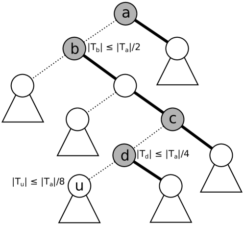
Figure 4: Illustration of Lemma 9. The grey nodes are the ones that $u$ are contributing to. For each grey apex node on the path from $u$ to the root, the number of contributing nodes grows by at least a factor of $2$.

We are now ready to bound the encoding time. First recall that we are using the word-RAM model with word size $c\log n$ for some sufficiently large constant $c$ such that the entire label $\ell(u)$ fits in one word. We are thus able to create the Elias $\gamma$ code of $k(u)$, $wc(u)$, $rld(u)$, and $M(u)$ in $O(1)$ time for each node $u$ using standard word operations.

We may assume that the children of each node is sorted by subtree size. Otherwise we can ensure this using e.g. bucket sort in $O(n)$ time.

Since all components of $aux(u)$ other than $k(u)$ can be calculated using a simple DFS-traversal in $O(n)$ time, we see that the total encoding time is dominated by the running time of Algorithm 1, Algorithm 2, and the time to construct $table(u)$ from the $a_{i}(u)$s. For Algorithm 2 we first observe that line 2 can be done in $O(1)$ time using the following approach:

1. Let $a$ be the integer resulting from setting the last $k(u)$ bits of the binary representation of $s$ to $0$.

2. If $a=s$, then return $s$.

3. Otherwise return $a+2^{k(u)}$

Each of the three steps can be done in $O(1)$ time using word operations. The rest of Algorithm 2 is a DFS-traversal, which runs in $O(n)$ time total. For the construction of $table(u)$, observe that all of $table(u)$ fits in a word, so we can calculate each $r_{i}(u)$ in $O(1)$ time. The total construction time over all nodes of $T$ is thus bounded by:

$$\begin{split}\sum_{u\in T}O(wc(u))&=O\!\left(\sum_{k=0}^{\left\lceil{\lg\lg n}\right\rceil}k\cdot|\{w\in T\mid wc(w)=k\}|\right)\\ &\leq O\!\left(\sum_{k=0}^{\left\lceil{\lg\lg n}\right\rceil}kn\cdot\frac{2^{k}}{2^{2^{k}}}\right)\\ &\leq O\!\left(n\cdot\sum_{k=0}^{\infty}\frac{k\cdot 2^{k}}{2^{2^{k}}}\right)\\ &=O(n)\ .\end{split}$$ (6)

Here, the second line follows by Lemma 9. For Algorithm 1 we see that the total time spent in the loop of line 1 to line 1 for all nodes $u\in T$ is bounded by

$$\sum_{u\in T}O(|children(u)|+wc(u))\ .$$

By (6) this is $O(n)$. The rest of Algorithm 1 spends time proportional to the length of the heavy path the function has been called with, which sums to $O(n)$ over all heavy paths. Note that line 1 is calculated in $O(1)$ time using Lemma 2.

By summing up the three different parts we see that the total encoding time of the labeling scheme is $O(n)$.

6.2 Decoding time

Using the conditions of Lemma 8 we will bound the decoding time of the labeling scheme:

Recall that we are able to decode each of $k(u)$, $wc(u)$, $rld(u)$, $apex(u)$, $leaf(u)$, $next(u)$, and $M(u)$ in $O(1)$ time. Doing this we also locate the beginning of $a_{1}(u)$ in the bit string (label). Let this bit position be denoted by $x$.

Knowing $x$, $M(u)$, and $wc(v)$ we can read the $wc(v)-1$st and $wc(v)$th entries of $table(u)$ in $O(1)$ time, since these are located exactly at bit positions $x+M(u)\cdot(wc(v)-2)$ and $x+M(u)\cdot(wc(v)-1)$. If $wc(v)=1$ we know that $a_{0}(u)=0$. Similarly we know that $wlsb(id(u),k(u))$ begins at bit position $x+M(u)\cdot(wc(u)-1)$ and consists of the remaining bits. We can do the same for $v$, thus decoding each relevant component of $\ell(u)$ and $\ell(v)$ can be done in $O(1)$ time.

The conditions 1.1, 1.2 and 2.1-4 can now be checked in $O(1)$ by using the corresponding values. For condition 1.3 we need to be able to find the smallest integer greater than $id(u)+lw(u)$ with at least $k(u)+next(u)$ trailing zeroes. Observe that $lw(u)=1+a_{wc(u)}(u)$ can be obtained in $O(1)$ time from $table(u)$ in the same manner as $a_{wc(v)}(u)$ was. Finding the smallest such integer can now be done in $O(1)$ time be using the same procedure as in the previous section.

This finishes the proof of Theorem 2.

Appendix A Adjacency labeling for trees explicitly listed as an open problem

Let $T_{n}$ denote the family of trees with $n$ nodes. In the quotes below ‘‘universal graph’’ is ‘‘induced universal’’.

Chung [27, emphasized on page 452-453] ‘‘What is the correct order of magnitude for $g_{v}(T_{n})$? [...] It would be of particular interest to sharpen the bounds for $g_{v}(T_{n})$ [...]’’

In [45, page 465] ‘‘Proving or disproving the existence of a universal graph with a linear number of nodes for the class of $n$-node trees is a central open problem in the design of informative labeling schemes.’’

In [49, page 592] ‘‘[...] prove an optimal bound for trees (up to an additive constant) which is still open.’’

In [19, page 143-144] ‘‘leaving open the question of whether trees enjoy a labeling scheme with $\log n+O(1)$ bit labels [...] In particular, for adjacency queries in trees, the current lower bound is $\log n$ and the upper bound is $\log n+O(\log^{*}n)$’’

In [48, page 42] ‘‘Induced-universal graph for n-node trees of $O(n)$ size?’’

In [57] ‘‘The question of matching upper and lower bounds for the sizes of the universal graphs for these families still remain open.’’ In this paper trees and graphs with bounded arboricity are two of the main families being considered.

In [44, page 132] ‘‘Proving or disproving the existence of an adjacency labeling scheme for trees using labels of size $\log n+O(1)$ remains a central open problem in the design of informative labeling schemes.’’

References

- [1] S. Abiteboul, S. Alstrup, H. Kaplan, T. Milo, and T. Rauhe. Compact labeling scheme for ancestor queries. SIAM J. Comput., 35(6):1295--1309, 2006.
- [2] S. Abiteboul, H. Kaplan, and T. Milo. Compact labeling schemes for ancestor queries. In Proc. of the 12th Annual ACM-SIAM Symp. on Discrete Algorithms (SODA), pages 547--556, 2001.
- [3] D. Adjiashvili and N. Rotbart. Labeling schemes for bounded degree graphs. In 41st International Colloquium on Automata, Languages, and Programming (ICALP), pages 375--386, 2014.
- [4] N. Alon and M. Capalbo. Sparse universal graphs for bounded-degree graphs. Random Structures & Algorithms, 31(2):123--133, 2007.
- [5] N. Alon and M. Capalbo. Optimal universal graphs with deterministic embedding. In Proc. of the 19th Annual ACM-SIAM Symp. on Discrete Algorithms (SODA), pages 373--378, 2008.
- [6] S. Alstrup, P. Bille, and T. Rauhe. Labeling schemes for small distances in trees. In Proc. of the 14th Annual ACM-SIAM Symp. on Discrete Algorithms (SODA), pages 689--698, 2003.
- [7] S. Alstrup, P. Bille, and T. Rauhe. Labeling schemes for small distances in trees. SIAM J. Discrete Math., 19(2):448--462, 2005. See also SODA’03.
- [8] S. Alstrup, C. Gavoille, E. B. Halvorsen, and H. Petersen. Simpler, faster and shorter labels for distances in graphs. In Proc. 27th Annual ACM-SIAM Symp. on Discrete Algorithms (SODA), pages 338--350, 2016.
- [9] S. Alstrup, H. Kaplan, M. Thorup, and U. Zwick. Adjacency labeling schemes and induced-universal graphs. In Proc. of the 47th Annual ACM Symp. on Theory of Computing (STOC), pages 625--634, 2015.
- [10] S. Alstrup and T. Rauhe. Improved labeling scheme for ancestor queries. In Proc. of the 13th Annual ACM-SIAM Symp. on Discrete Algorithms (SODA), pages 947--953, 2002.
- [11] S. Alstrup and T. Rauhe. Small induced-universal graphs and compact implicit graph representations. In Proc. 43rd Annual Symp. on Foundations of Computer Science (FOCS), pages 53--62, 2002.
- [12] L. Babai, F. R. K. Chung, P. Erdös R. L. Graham, and J. Spencer. On graphs which contain all sparse graphs. Ann. discrete Math., 12:21--26, 1982.
- [13] F. Bazzaro and C. Gavoille. Localized and compact data-structure for comparability graphs. Discrete Mathematics, 309(11):3465--3484, 2009.
- [14] L. W. Beineke and R. T. Wilson. A survey of recent results on tournaments. Recent advances in Graph Theory. Proc. Prague Symp,, pages 31--48, 1975.
- [15] S. N. Bhatt, F. R. K. Chung, F. T. Leighton, and A. L. Rosenberg. Optimal simulations of tree machines. In 27th Annual Symp. on Foundations of Computer Science (FOCS), pages 274--282, 1986.
- [16] S. N. Bhatt, F. R. K. Chung, F. T. Leighton, and A. L. Rosenberg. Universal graphs for bounded-degree trees and planar graphs. SIAM J. Discrete Math., 2(2):145--155, 1989.
- [17] B. Bollobás and A. Thomason. Graphs which contain all small graphs. European J. of Combinatorics, 2(1):13--15, 1981.
- [18] J. A. Bondy. Pancyclic graphs I. J. Combinat. theory B, 11:80--84, 1971.
- [19] N. Bonichon, C. Gavoille, and A. Labourel. Short labels by traversal and jumping. In Structural Information and Communication Complexity, pages 143--156. Springer, 2006. Include proof for binary trees and caterpillars.
- [20] N. Bonichon, C. Gavoille, and A. Labourel. An efficient adjacency scheme for bounded degree trees. Preprint version, July 2007. Version recieved from C. Gavoille. Include proof for bounded degree.
- [21] N. Bonichon, C. Gavoille, and A. Labourel. Short labels by traversal and jumping. Electronic Notes in Discrete Mathematics, 28:153--160, 2007. State without proof the bounded degree result.
- [22] M. A. Breuer. Coding the vertexes of a graph. IEEE Trans. on Information Theory, IT--12:148--153, 1966.
- [23] M. A. Breuer and J. Folkman. An unexpected result on coding vertices of a graph. J. of Mathemathical analysis and applications, 20:583--600, 1967.
- [24] S. Butler. Induced-universal graphs for graphs with bounded maximum degree. Graphs and Combinatorics, 25(4):461--468, 2009.
- [25] G. Chartrand, H. V. Kronk, and C. E. Wall. The point-arboricity of a graph. Israel J. of Mathematics, 6(2):169--175, 1968.
- [26] V. D. Chepoi, F. F. Dragan, and Y. Vaxès. Distance and routing labeling schemes for non-positively curved plane graphs. J. of Algorithms, 61(2):60--88, 2006.
- [27] F. R. K. Chung. Universal graphs and induced-universal graphs. J. of Graph Theory, 14(4):443--454, 1990.
- [28] F. R. K. Chung and R. L. Graham. On graphs which contain all small trees. J. of combinatorial theory, Series B, 24(1):14--23, 1978.
- [29] F. R. K. Chung and R. L. Graham. On universal graphs. Ann. Acad. Sci., 319:136--140, 1979.
- [30] F. R. K. Chung and R. L. Graham. On universal graphs for spanning trees. J. London Math. Soc., 27:203--211, 1983.
- [31] F. R. K. Chung, R. L. Graham, and D. Coppersmith. On trees which contain all small trees. In The theory and applications of graphs, pages 265--272. John Wiley and Sons, 1981.
- [32] F. R. K. Chung, R. L. Graham, and N. Pippenger. On graphs which contain all small trees ii. Colloquia Mathematica, pages 213--223, 1976.
- [33] E. Cohen, H. Kaplan, and T. Milo. Labeling dynamic XML trees. SIAM J. Comput., 39(5):2048--2074, 2010.
- [34] L. J. Cowen. Compact routing with minimum stretch. J. of Algorithms, 38:170--183, 2001. See also SODA’91.
- [35] S. Dahlgaard, M. B. T. Knudsen, and N. Rotbart. A simple and optimal ancestry labeling scheme for trees. In Automata, Languages, and Programming - 42nd International Colloquium, ICALP 2015, Kyoto, Japan, July 6-10, 2015, Proceedings, Part II, pages 564--574, 2015.
- [36] Y. Dodis, M. Pǎtraşcu, and M. Thorup. Changing base without losing space. In Proc. of the 42nd Annual ACM Symp. on Theory of Computing (STOC), pages 593--602, 2010.
- [37] T. Eilam, C. Gavoille, and D. Peleg. Compact routing schemes with low stretch factor. J. of Algorithms, 46(2):97--114, 2003.
- [38] P. Elias. Universal codeword sets and representations of the integers. IEEE Transactions on Information Theory, 21(2):194--203, 1975.
- [39] L. Esperet, A. Labourel, and P. Ochem. On induced-universal graphs for the class of bounded-degree graphs. Inf. Process. Lett., 108(5):255--260, 2008.
- [40] A. Farzan and J. I. Munro. Succinct encoding of arbitrary graphs. Theoretical Computer Science, 513:38--52, 2013.
- [41] A. Farzan and J. I. Munro. A uniform paradigm to succinctly encode various families of trees. Algorithmica, 68(1):16--40, 2014.
- [42] P. C. Fishburn. Minimum graphs that contain all small trees. Ars Combinat., 25:133--165, 1985.
- [43] P. Fraigniaud and C. Gavoille. Routing in trees. In International Colloquium on Automata, Languages and Programming (ICALP), pages 757--772, 2001.
- [44] P. Fraigniaud and A. Korman. On randomized representations of graphs using short labels. In Proc. of the 21st Annual Symp. on Parallelism in Algorithms and Architectures (SPAA), pages 131--137, 2009.
- [45] P. Fraigniaud and A. Korman. Compact ancestry labeling schemes for XML trees. In Proc. of the 21st annual ACM-SIAM Symp. on Discrete Algorithms (SODA), pages 458--466, 2010.
- [46] P. Fraigniaud and A. Korman. An optimal ancestry scheme and small universal posets. In Proc. of the 42nd Annual ACM Symp. on Theory of Computing (STOC), pages 611--620, 2010.
- [47] J. Friedman and N. Pippenger. Expanding graphs contain all small trees. Combinatorica, 7:71--76, 1987.
- [48] C. Gavoille. Progress and challenges for labeling schemes. Presented at Advances in Distributed Graph Algorithms (ADGA), 2012.
- [49] C. Gavoille and A. Labourel. Shorter implicit representation for planar graphs and bounded treewidth graphs. In Algorithms--ESA, pages 582--593. Springer, 2007.
- [50] C. Gavoille and C. Paul. Optimal distance labeling for interval graphs and related graphs families. SIAM J. Discrete Math., 22(3):1239--1258, 2008.
- [51] C. Gavoille and D. Peleg. Compact and localized distributed data structures. Distributed Computing, 16(2-3):111--120, 2003.
- [52] C. Gavoille, D. Peleg, S. Pérennes, and R. Raz. Distance labeling in graphs. J. of Algorithms, 53(1):85 -- 112, 2004. See also SODA’01.
- [53] R. L. Graham and H. O. Pollak. On embedding graphs in squashed cubes. In Lecture Notes in Mathematics, volume 303, pages 99--110. Springer-Verlag, 1972.
- [54] A. Gupta, R. Krauthgamer, and J. R. Lee. Bounded geometries, fractals, and low-distortion embeddings. In 44th Annual Symp. on Foundations of Computer Science (FOCS), pages 534--543, 2003.
- [55] A. Gupta, A. Kumar, and R. Rastogi. Traveling with a pez dispenser (or, routing issues in mpls). SIAM J. on Computing, 34(2):453--474, 2005. See also FOCS’01.
- [56] P. L. Hammer and A. K. Kelmans. On universal threshold graphs. Combinatorics, Probability and Computing, 3:327--344, 9 1994.
- [57] S. Kannan, M. Naor, and S. Rudich. Implicit representation of graphs. SIAM J. Disc. Math., 5(4):596--603, 1992. See also STOC’88.
- [58] H. Kaplan and T. Milo. Short and simple labels for distances and other functions. In 7nd Work. on Algo. and Data Struc., pages 246--257, 2001.
- [59] H. Kaplan, T. Milo, and R. Shabo. A comparison of labeling schemes for ancestor queries. In Proc. of the 13th Annual ACM-SIAM Symp. on Discrete Algorithms (SODA), pages 954--963, 2002.
- [60] M. Katz, N. A. Katz, A. Korman, and D. Peleg. Labeling schemes for flow and connectivity. SIAM J. Comput., 34(1):23--40, 2004. See also SODA’02.
- [61] A. Korman. Labeling schemes for vertex connectivity. ACM Trans. Algorithms, 6(2):39:1--39:10, 2010.
- [62] A. Korman and D. Peleg. Labeling schemes for weighted dynamic trees. Inf. Comput., 205(12):1721--1740, 2007.
- [63] R. Krauthgamer and J. R. Lee. Algorithms on negatively curved spaces. In 47th Annual Symp. on Foundations of Computer Science (FOCS), pages 119--132, 2006.
- [64] L. Lovasz. On decomposition of graphs. Studia Sci. Math. Hungar, 1:237--238, 1966.
- [65] V. V. Lozin. On minimal universal graphs for hereditary classes. Discrete Math. Appl., 7(3):295--304, 1997.
- [66] V. V. Lozin and G. Rudolf. Minimal universal bipartite graphs. Ars Comb., 84, 2007.
- [67] J. W. Moon. On minimal -universal graphs. Proc. of the Glasgow Mathematical Association, 7(1):32--33, 1965.
- [68] J. W. Moon. Topics on tournaments. Holt, Rinehart and Winston, 1968.
- [69] J. H. Müller. Local structure in graph classes. PhD thesis, Georgia Institute of Technology, 1988.
- [70] J. I. Munro, R. Raman, V. Raman, and S. Srinivasa Rao. Succinct representations of permutations and functions. Theor. Comput. Sci., 438:74--88, 2012.
- [71] J. I. Munro and V. Raman. Succinct representation of balanced parantheses, static trees and planar graphs. In 38th Annual Symp. on Foundations of Computer Science (FOCS), pages 118--126, 1997.
- [72] L. Nebesky. On tree-complete graphs. Casopis Pest. Mat., 100:334--338, 1975.
- [73] R. Otter. The number of trees. Annals of Mathematics. Second Series, 49(3):583--599, 1948.
- [74] T. D. Parsons and Tomaž Pisanski. Exotic -universal graphs. J. of Graph Theory, 12(2):155--158, 1988.
- [75] M. Pǎtraşcu. Succincter. In Proc. 49th Annual Symp. on Foundations of Computer Science (FOCS), pages 305--313, 2008.
- [76] D. Peleg. Informative labeling schemes for graphs. In Proc. 25th Symp. on Mathematical Foundations of Computer Science, pages 579--588, 2000.
- [77] D. Peleg. Proximity-preserving labeling schemes. J. Graph Theory, 33(3):167--176, 2000.
- [78] T. Pisanski. Universal commutator graphs. Discrete Math., 78(1-2):155--156, 1989.
- [79] R. Rado. Universal graphs and universal functions. Acta. Arith., 9:331--340, 1964.
- [80] N. Santoro and R. Khatib. Labeling and implicit routing in networks. The computer J., 28:5--8, 1985.
- [81] E. R. Scheinerman and J. Zito. On the size of hereditary classes of graphs. J. of Combinatorial Theory, Series B, 61(1):16 -- 39, 1994.
- [82] D. D. Sleator and R. E. Tarjan. A data structure for dynamic trees. J. of Computer and System Sciences, 26(3):362 -- 391, 1983.
- [83] J. P. Spinrad. Efficient Graph Representations, volume 19 of Fields Institute Monographs. AMS, 2003.
- [84] A. Takahashi and S. Ueno Y. Kajitani. Universal graphs for graphs with bounded path-width. IEICE Trans. Fundamentals, E78--A(4):458--462, 1995.
- [85] M. Talamo and P. Vocca. Compact implicit representation of graphs. In Graph-Theoretic concepts in Computer Science, 24th international workshop (WG), pages 164--176, 1998.
- [86] K. Talwar. Bypassing the embedding: algorithms for low dimensional metrics. In Proc. of the 36th Annual ACM Symp. on Theory of Computing (STOC), pages 281--290, 2004.
- [87] M. Thorup. Compact oracles for reachability and approximate distances in planar digraphs. J. ACM, 51(6):993--1024, 2004. See also FOCS’01.
- [88] M. Thorup and U. Zwick. Approximate distance oracles. In Proc. of the 13th annual ACM-SIAM Symp. on Theory of Computing (STOC), pages 1--10, 2001.
- [89] M. Thorup and U. Zwick. Approximate distance oracles. J. of the ACM, 52(1):1--24, 2005. See also STOC’01.
- [90] Wikipedia. Implicit graph --- wikipedia, the free encyclopedia, 2013. [Online; accessed 15-February-2014].
- [91] P. M. Winkler. Proof of the squashed cube conjecture. Combinatorica, 3(1):135--139, 1983.