Structure, thermodynamic properties, and phase diagrams of few colloids confined in a spherical pore

Abstract

We study a system of few colloids confined in a small spherical cavity by event driven molecular dynamics simulations in the canonical ensemble. The colloidal particles interact through a short range square-well potential, which takes into account the basic elements of attraction and excluded-volume repulsion of the interaction among colloids. We analyze the structural and thermodynamic properties of this few-body confined system in the framework of the theory of inhomogeneous fluids. Pair correlation functions and density profiles across the cavity are used to determine the structure of the system and the spatial characteristics of its inhomogeneities. Pressure on the walls, internal energy and surface quantities such as surface tension and adsorption are also analyzed for the whole range of densities, temperatures and number of particles considered. We have characterized the structure of systems from 2 to 6 confined particles as function of density and temperature, identifying the distinctive qualitative behaviors all over the thermodynamic plane $T-\rho$ in a few-particle equivalence to phase diagrams of macroscopic systems. Applying the extended law of corresponding states the square well interaction is mapped to the Asakura-Oosawa model for colloid-polymer mixtures. We link explicitly the temperature in the confined square-well fluid to the equivalent packing fraction of polymers in the Asakura-Oosawa model. Using this approach we study the confined system of few colloids in a colloid-polymer mixture.

I Introduction

During last decades colloid physics has been one of the areas of more intensive activity in the field of soft matter. Colloidal dispersions have wide and well known applications in the chemical, pharmaceutical, medical and food industries.Wang et al. (2011) Moreover, colloids posses certain properties that make them good model systems for basic research.Weeks (2012); Sacanna et al. (2010); Meng et al. (2010); Lu et al. (2008) The size of colloidal particles, in the range $1nm-10\mu m$, make possible its direct experimental observation giving rise to beautiful and conclusive experiments. It has enabled the direct study of phase transitions like the gas-liquid, the gas-solid and gelation ones, which is impossible for simple fluids.Wang et al. (2012); Aarts, Schmidt, and Lekkerkerker (2004); Anderson and Lekkerkerker (2002); de Hoog et al. (2001)

Some colloidal suspensions behave like hard spheres (HS) where the unique relevant feature of the interacting potential is the repulsion length $\sigma$ (particle diameter), related with the excluded volume.Royall, Poon, and Weeks (2013); Royall, Louis, and Tanaka (2007) Free energy and pressure of few HS colloids confined in a spherical pore were studied recently by molecular dynamics and theoretical approaches.Urrutia and Pastorino (2014); Urrutia and Castelletti (2012); Urrutia (2011) In several cases, it is necessary to complement this hard-core repulsion with an attractive, short-range interaction, to properly describe the potential between colloidal particles. For this purpose, the square-well (SW) potential has been utilized.Acedo and Santos (2001) Systems of particles that interact through SW potential have been investigated extensively, exploiting the fact that its simplicity enables to study both, in bulk and in confinement, not only through Monte Carlo and molecular dynamics simulations, but also with analytic approaches. SW system is the simplest interaction model that includes a repulsive core and an attractive well with tunable range, giving rise to phase transitions and coexistence regions. The thermodynamic properties, phases coexistence,Li et al. (2014); Rivera-Torres et al. (2013); Espíndola-Heredia, Río, and Malijevský (2009); Vortler, Schafer, and Smith (2008); López-Rendón, Reyes, and Orea (2006); Kiselev, Ely, and Elliott (2006); Liu, Garde, and Kumar (2005) structure,Khanpour (2011) crystallization, glassy behaviorHartskeerl (2009) and percolation phenomenaNeitsch and Klapp (2013) of short-range SW fluids were extensively studied in bulk. Properties of inhomogeneous SW systems at free interphases and in confinement, were also studied.Armas-Pérez, Quintana-H, and Chapela (2013); Neitsch and Klapp (2013); Huang et al. (2010); Jana, Singh, and Kwak (2009); Zhang and Wang (2006) Molecular dynamics studies to obtain bulk free energy of short range SW particles were performed recently.Rivera-Torres et al. (2013); Pagan and Gunton (2005) Pressure on the wall and structural properties were studied for two SW particles in a spherical cavity.Urrutia and Castelletti (2011a) Liquid-vapor coexistence of SW fluid confined in cylindrical poresReyes (2012) and short range SW potential in the context of effective interactions among proteinsDuda (2009) were also studied.

Adding long, flexible, non-adsorbing polymer chains to a colloidal suspension causes changes on the phase behavior of the colloidal system. We shall focus on the rather simple Asakura-Oosawa model (AO) for colloid-polymer mixtures.Asakura and Oosawa (1954, 1958) In this model based on HS-type interactions, the colloids are taken as hard spheres with diameter $\sigma$. The polymers with diameter $\sigma_{p}$ are excluded by a center of mass distance of $\frac{\sigma+\sigma_{p}}{2}$ from the colloids. However, polymers are treated as non-interacting particles that can overlap. This kind of interactions leads to an effective attractive two-body potential between colloids, due to an unbalanced osmotic pressure arising from depletion.Israelachvili (2011) Although, for a small enough diameters ratio $\sigma_{p}/\sigma$ the two-body effective potential has a short-range attractive well, and the three- and many-body potentials are null.Vrij (1976) In addition, when $\sigma_{p}/\sigma$ is small the main features of the colloid-colloid effective pair potential are similar to the simpler SW potential. Studies of the AO model with different values of diameter ratio have shown interesting properties in bulk, as glassy states and demixing,Germain and Amokrane (2007); López de Haro et al. (2015) as well as in confinement.Binder, Virnau, and Statt (2014); Winkler et al. (2013); Statt et al. (2012)

In this work, we study thoroughly highly confined colloids in spherical pores, that show different demeanor as compared to their bulk counterparts. The confining cavity (thought as a nanopore) breaks the translational symmetry of a system and causes the appearance of spatial variations. Even farther from bulk case, our aim is to work with low number of particles and a system size comparable to its constituents elements. This implies that we are far away from thermodynamic limit. Nevertheless we work in the frame of statistical mechanics. In addition, low $N$ systems allow for analytic solutions at some degree, thus letting us to make a direct comparison between theory and simulation results. On this line, we study the system of few short-range colloids in a hard-wall spherical pore. The pure colloidal suspension is studied by event-driven molecular dynamics simulations using the SW model in a wide range of number densities and relevant temperatures. We also map the simulated system to a colloid-polymer mixture in a spherical pore. In this case we adopt the AO model and consider the case of small ratio $\sigma_{p}/\sigma$. We connect the short-range SW potential and the AO model by adopting the effective short-range colloid-colloid pair potential through an extended corresponding-states law, following that of Noro and Frenkel.Noro and Frenkel (2000); Valadez-Pérez et al. (2012)

The paper is organized as follows, in Sec. II we provide details of the interaction model and the statistical mechanics theoretical grounds for both few body systems: colloidal suspensions and colloid-polymer mixtures in pores. In Sec. III we present the simulation technique and the way in which we obtain canonical ensemble simulations at constant temperature. Sec. IV is devoted to present the density profiles, pair correlation functions, thermodynamics properties and phase diagrams of systems of 2, 3, 4, 5 and 6 colloidal particles in a spherical cavity. There, we analyze the results for the simulated SW system and also for the equivalent AO system, whenever possible. We present a final discussion and conclusions in Section V.

II Theoretical background

We study a system of $N$ colloidal particles of diameter $\sigma$ confined in a spherical cavity of radius $R_{o}$, at constant temperature $T$. The particles interact with the cavity through a hard wall potential which prevents them from escaping to the outside. Thus, the effective radius of the cavity is $R_{\textrm{eff}}\equiv R_{o}-\sigma/2$, which represents the maximum possible distance between the center of the cavity and the center of each colloid. The temperature of the fluid is determined by the wall temperature $T$, which is fixed. We adopt the effective volume $V=4\pi R_{\textrm{eff}}/3$ to measure the size of the available space for particles and consistently define the mean number density $\rho=N/V$.

Given that we deal with a small number of colloids, the ensembles equivalence does not apply. The statistical mechanical and thermodynamic properties of the system with constant $N$ and $T$ is obtained from its canonical partition function (CPF), $Q_{N}$. One actually works with the configuration integral (CI), given that kinetic degrees of freedom integrate trivially. Thus, the CPF reads

$$Q_{N}=\frac{1}{N!}\Lambda^{-3N}Z_{N}\>.$$ (1)

Here $\Lambda$ is the thermal de Broglie wavelength and $Z_{N}$ is the CI of the system. For pair interacting particles $Z_{N}=\int_{V}\prod_{<jk>}e_{jk}\,d\mathbf{r}^{N}$, where the Boltzmann factor for the $j,k$-pair is $e_{jk}=\exp\left[-\beta\phi\left(r_{jk}\right)\right]$, $r_{jk}$ is the distance between both particles, $\phi$ is the pair potential and the inverse temperature is defined as $\beta=1/kT$, with $k$ the Boltzmann constant. For a system in stationary conditions with fixed $N$ and $T$ the Helmholtz free energy ($F$) reads

$$F=U-TS=-\beta^{-1}\ln Q_{N}\>,$$ (2)

where $U$ is the system energy and $S$ its entropy. The reversible work done at constant temperature, to change the cavity radius between states $a$ and $b$ is

$$F_{b}-F_{a}=-\intop_{a}^{b}P_{w}dV\>,$$ (3)

with $dV=A\,dR_{\textrm{eff}}$. Here, $P_{w}$ is the pressure on the spherical wall which is an EOS of the system. The derivative of Eq. (3) at constant $T$ gives the pressure on the wall through

$$P_{w}=-A^{-1}dF/dR_{\textrm{eff}}\>,$$ (4)

which meets the exact relation known as contact theoremHansen and McDonald (2006); Blokhuis and Kuipers (2007)

$$\beta P_{w}=\rho\left(R_{\textrm{eff}}\right)\>.$$ (5)

In this ideal gas-like relation, $\rho\left(R_{\textrm{eff}}\right)$ is the value that takes the density profile at contact with the wall. This extended version of the contact theorem for planar walls applies to curved walls of constant curvature (spheres and cylinders), for both open and closed systems. A complete discussion of the presented statistical mechanical approach for few-body confined system that includes other properties, such as the energy, may be found in Refs. Urrutia and Castelletti (2011a); Paganini (2014).

Here we consider the confined colloids as particles that interact through the square well potential:

$$\phi_{\textrm{SW}}\bigl{(}r\bigr{)}=\begin{cases}\infty&\textrm{if }0<r<\sigma,\\ -\varepsilon&\textrm{if }\sigma<r<\left(1+\lambda\right)\sigma,\\ 0&\textrm{if }r>\left(1+\lambda\right)\sigma,\end{cases}$$ (6)

where $\varepsilon>0$. In this work, we study the short-range SW system with $\lambda=0.1$. The bulk and interfacial properties of short-range SW fluids have been studied elsewhere.Valadez-Pérez et al. (2012); Neitsch and Klapp (2013); López-Rendón, Reyes, and Orea (2006) For reference, we note that the bulk SW system with $\lambda=0.1$ has a metastable fluid-vapor transition with critical temperature $T=0.47\,\varepsilon/k$ and density $\rho=0.47\,\sigma^{-3}$.Valadez-Pérez et al. (2012); Liu, Garde, and Kumar (2005)

Statistical mechanics of the semi-grandcanonical confined AO system

In the AO model a particular colloid-polymer mixture is characterized by the ratio $q=\frac{\sigma_{p}}{\sigma}$. The diameter of the polymer coil is given by $\sigma_{p}=2R_{g}$ with $R_{g}$ the radius of gyration of the polymer. The effect of temperature on $R_{g}$ was studied in Ref.Taylor, Evans, and Royall (2012). In the AO model the temperature does not play any relevant role and thus we consider $T$ as fixed to fix $\sigma_{p}$. We consider the mixture of $N$ colloidal particles and polymers at chemical potential $\mu_{p}$, at a given temperature. The spherically confined system of colloids is such that the polymers, which are much smaller than colloidal particles, can freely pass through the semipermeable wall that only constrains the colloids into the pore. The colloid-polymer AO mixture is an inhomogeneous system that can be analyzed in the semi-grand canonical ensemble. Its partition function is

$$\Xi_{m}=\frac{\Lambda^{-3N}}{N!}\sum_{N_{p}}\frac{z_{p}^{N_{p}}}{N_{p}!}Z_{N,N_{p}}\>,$$ (7)

with $z_{p}=\varLambda_{p}^{-3}e^{\beta\mu_{p}}$, $\varLambda_{p}$ the thermal de Broglie length of the polymer and $\varLambda$ the same magnitude for the colloidal particle. $Z_{N,N_{p}}$ is the CI of the mixture with the $N$ colloids, whose centers are constrained to the pore with volume $V=4\pi R_{\textrm{eff}}^{3}/3$, and the $N_{p}$ polymers in the larger volume $V_{p}$. In the Appendix A it is shown that Eq. (7) transforms to

$$\Xi_{m}=\Xi_{p}^{h}\frac{\Lambda^{-3N}}{N!}e^{-\bigl{(}\rho_{p}v_{exc}N\bigr{)}}Z_{N}^{(\textrm{AO})}\>,$$ (8)

where $\rho_{p}$ is the mean number density of the pure (homogeneous) polymer system and $Z_{N}^{(\textrm{AO})}$ is the CI of $N$ confined colloids interacting trough the effective pair-potential $\phi_{\textrm{AO}}$. $v_{exc}$ stands for the excluded volume defined in the Appendix A. Given two colloids at a distance $r$ apart, $\phi_{\textrm{AO}}(r)$ is infinity for $r<\sigma$ and it is zero for $r>\sigma(1+q)$. In the attractive well region $\sigma<r<\sigma(1+q)$ it is

$$\beta\phi_{\textrm{AO}}\bigl{(}x\bigr{)}=\!-\eta_{p}\left(1+q^{-1}\right)^{3}\!\biggl{[}1-\frac{3x}{2\left(1+q\right)}+\frac{x^{3}}{2\left(1+q\right)^{3}}\biggr{]},$$ (9)

where $x=r/\sigma$ and $\eta_{p}=\rho_{p}\left(\pi\sigma_{p}^{3}/6\right)$ is the packing fraction of the polymers (note that $\eta_{p}$ takes any positive value). The expression in Eq. (9) is minus $\rho_{p}$ times the volume of intersection of two spheres of radius $\sigma\left(1+q\right)/2$ whose centers are at a distance $r$.

For the thermodynamic analysis of the AO model we use as reference the pure polymer system (an ideal-gas) with the grand-free energy given by $\Omega_{p}^{h}=U_{p}^{h}-TS_{p}^{h}-\mu_{p}N_{p}^{h}$ (with $N_{p}^{h}=\rho_{p}V_{p}$). The semi-grand free energy of the mixture is $\Omega_{m}=U_{m}-TS_{m}-\mu_{p}N_{p}$ and given that the system is athermal its energy is purely kinetic $U_{m}=\frac{3}{2}kTN+\frac{3}{2}kTN_{p}$. We define

$$F_{\textrm{AO}} = \Omega_{m}-\Omega_{p}^{h}\>,$$ (10)

$$= U_{c}-T\left(S_{m}-S_{p}^{h}\right)+\left(3kT/2-\mu_{p}\right)\Delta N_{p}\,,$$

with $U_{c}=\frac{3}{2}kTN$, $\Delta N_{p}=N_{p}-N_{p}^{h}$ and $\Omega=-\beta\ln\Xi$. Here, $F_{\textrm{AO}}$ is the free energy of the confined colloids in the polymer solution as an excess over the pure polymer system. The pressure exerted by the colloids on the wall, the osmotic pressure, is

$$P_{w}=-A^{-1}dF_{\textrm{AO}}/dR_{\textrm{eff}}\>,$$ (11)

and relates with the colloids density distribution $\rho\left(\mathbf{r}\right)$ through the contact theorem

$$\beta P_{w}=\rho\left(R_{\textrm{eff}}\right)\>.$$ (12)

Eqs. (11, 12) are essentially the same that Eqs. (4, 5) but the meaning of each magnitude corresponds to different systems.

Extended law of corresponding states

The short range SW potential and its capability to describe any short range potential (universality) was proposed by Noro and Frenkel in his extended version of the corresponding state law.Noro and Frenkel (2000) It is based on a mapping between different systems using three parameters: the effective hard core diameter, the well depth and the adimensional second virial coefficient. The later was proposed as a measure for the range of the attractive part of the potential. The scheme was used previously for studying the critical properties of the liquid-vapor transition for interaction models including Lennard-Jones and Hard-Yukawa.Noro and Frenkel (2000); Germain and Amokrane (2010); Gnan, Zaccarelli, and Sciortino (2012). Recently, it was employed to analyze the behavior of proteins in water solutions.Valadez-Pérez et al. (2012)

It is important to note that we apply the law of corresponding states to analyze confined systems composed by few particles. This is very unusual and thus we made some checks to validate the overall approach that will be shown in Sec. IV. Our application of the law for hard-core systems is based on the use of two natural scales: the hard core diameter for the length scale and the depth of the attractive well for the temperature scale. The reduced second virial coefficient is given by $B=-\frac{1}{2b_{2}}\int\left[\exp\left(-\beta\phi\bigl{(}r\bigr{)}\right)-1\right]\,d\mathbf{r}$ with $b_{2}=2\pi\sigma^{3}/3$. For the SW system, this gives explicitly:

$$B_{\textrm{sw}}=1-\left(e^{1/T^{*}}-1\right)3\lambda\left(1+\lambda+\lambda^{2}/3\right)\>,$$ (13)

where we have introduced the adimensional temperature $T^{*}=Tk/\varepsilon$ (its inverse is $\beta^{*}=1/T^{*}$). In the limit of a very narrow well, the SW potential reaches the Baxter’s sticky spheres limit with

$$B=1-1/4\tau\>.$$

Here $\tau$ (that grows monotonically with $T$) plays the role of temperature.Hansen-Goos, Miller, and Wettlaufer (2012); Charbonneau and Frenkel (2007) In the AO model the effective colloid-colloid second virial coefficient $B_{\textrm{AO}}$ is not analytically integrable. To relate $B_{\textrm{sw}}$ with $B_{\textrm{AO}}$, we link the width of the wells by $q=2\lambda$. This mimics the fact that $\beta\phi_{\textrm{AO}}\bigl{(}x\bigr{)}$ is deeper near the hard-core of the particle. For the AO system with corresponding well-range $q=2\lambda$, the relation $B_{\textrm{AO}}\left(\eta_{p},q=2\lambda\right)=B_{\textrm{sw}}\left(T^{*},\lambda\right)$ fixes the pair of equivalent states $T^{*}\longleftrightarrow\eta$.

$q=2\lambda$	$c_{1}$	$c_{2}$	$c_{3}$
$0.2$	$0.886964$	$0.22724$	$0.015641$
$0.15$	$0.884047$	$0.29956$	$0.013871$
$0.1$	$0.876335$	$0.44847$	$0.012614$
$0.05$	$0.847353$	$0.92875$	$0.013498$

Table 1: Fitting parameters for the SW-AO mapping. They relate $T^{*}$ of the SW system to the value of the packing fraction $\eta_{p}$ (see Section II) in the corresponding state of the AO system.

This mapping allows the numerical evaluation of $B_{\textrm{AO}}$ and the fit of a nearly linear relation between $1/T^{*}$ and $\eta$ for several values of $\lambda$. The coefficients obtained for the fitted function

$$\frac{1}{T^{*}}=\frac{2}{3}\left(1+1.5q^{-1}\right)\sum_{i=1}^{3}c_{i}h_{i}\>,$$ (14)

with $h_{1}=\eta_{p}$, $h_{2}=\eta_{p}^{2}$ and $h_{3}=\eta_{p}/(0.1+\eta_{p})$, are shown in Table 1.

$\tau$	$T^{*}\,\left(\textrm{SW, }\lambda=0.1\right)$	$\eta_{p}\,\left(\textrm{AO, }q=0.2\right)$
$0.0051$	$0.2$	$0.81071$
$0.0675$	$0.4$	$0.43466$
$0.1758$	$0.6$	$0.29597$
$0.3033$	$0.8$	$0.22369$
$0.4395$	$1.0$	$0.17939$
$0.5805$	$1.2$	$0.14950$

Table 2: Law of corresponding states for short range potentials of SW and AO types. First column presents the sticky-sphere temperature parameter $\tau$. Second and third columns show the temperature for the SW particles and the corresponding packing fraction of polymer for the AO model, respectively.

The case $\lambda=0.1$ and $q=0.2$ is presented in Table 2, where corresponding values of sticky temperature, adimensional temperature of the SW system and polymer packing fraction are shown.

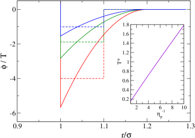
Figure 1: Corresponding states between SW potential (dashed lines) and AO effective potential (full lines) for $\lambda=0.1$ and $q=0.2$. From bottom to top, the inverse of the packing fraction (temperature) for AO (SW) curves are $\eta_{p}^{-1}=1.5$, $3$ and $5.5$ ($T^{*}=0.25$, $0.53$ and $0.985$). The inset presents the nearly linear relation between $T^{*}$ and $\eta_{p}$ used to map the SW system to the AO model.

In Fig. 1 we present the SW potential and the effective AO potential that yields corresponding states for several temperatures and polymer packing fraction ($\lambda=0.1$ and $q=0.2$). The inset shows the simple relation between the temperature of the SW particles and the corresponding packing fraction of polymers for the AO colloid-polymer mixture expressed in Eq. (14). In Sec. IV, the overall approach will be used to analyze the spherically confined system of few colloids in a colloid-polymer mixture.

III Simulation method

The statistical mechanical equivalence between different ensembles does not apply to few-body systems. Therefore, simulation and statistical mechanical approaches should correspond to the same physical constraints, to ensure comparable results. In this work, we focus on a system at constant temperature, fixed volume and number of particles. It corresponds to a canonical ensemble, and thus one assumes a Maxwell-Boltzmann velocity distribution. Accordingly, the simulations have to include a thermostating mechanism that ensures constant temperature and Maxwell-Boltzmann velocity distribution.

Molecular dynamics simulations of few SW confined in a spherical cavity were performed with a standard event-driven algorithm (EDMD).Allen and Tildesley (1987) Constant temperature was achieved by using a thermal-wall thermostat, which changes the velocity of the particle colliding with the wall by means of a velocity distribution compatible with canonical ensemble for a given temperature $T$. Thermal walls show certain features different from those thermostats that act over the entire system volume that were discussed in detail in a previous work.Urrutia and Pastorino (2014)

For the particle interactions, we take into account different types of events. Namely, particle-particle collision and particle-wall collision. Among particle-particle collisions there is a further division between core and field events, each one related with a discontinuous step in $\phi_{\textrm{SW}}\bigl{(}r\bigr{)}$. The usual EDMD algorithm was used, in which the particle moves with rectilinear and constant-velocity dynamics, between particle collisions.Allen and Tildesley (1987); López-Rendón, Reyes, and Orea (2006) In order to discriminate particle-particle collisions we used the logical structure of Alder and Wainwright.Alder and Wainwright (1959)

The time to collision of particle $i$ with particle $j$ is calculated as:

$$t_{ij,k}=\frac{-b_{ij}\pm\left[b_{ij}^{2}-v_{ij}^{2}\left(r_{ij}^{2}-\sigma_{k}^{2}\right)\right]^{1/2}}{v_{ij}^{2}}\>,$$ (15)

where $\mathbf{r}_{ij}\equiv\mathbf{r}_{i}-\mathbf{r}_{j}$ and $\mathbf{v}_{ij}\equiv\mathbf{v}_{i}-\mathbf{v}_{j}$ are the relative positions and velocities of the particle pair, respectively. Two collision distances $\sigma_{k}$ are considered $\sigma_{1}=\sigma$ and $\sigma_{2}=\sigma\left(1+\lambda\right)$. The parameter $b_{ij}\equiv\mathbf{r}_{ij}\cdot\mathbf{v}_{ij}$ must be negative if the particles are approaching each other and positive otherwise, and we consider only the positive values of $t_{ij,k}$. The Eq. (15) is obtained by imposing the condition $|\mathbf{r}_{ij}+\mathbf{v}_{ij}t_{ij,k}|=\sigma_{k}$ at collision time $t_{ij,k}$. The $\pm$ appears because both results are possible, given the right conditions: the “$-$” sign applies for particles approaching from outside regions ($r_{ij}>\sigma_{2}$), and a “$+$” sign, on the other hand, is for particles already inside the attractive well region ($r_{ij}<\sigma_{2}$) and getting outside of it, by receding.

An ordered list of events, with increasing collision times $t_{ij,k}$ is generated. Between collisions, the particles move with $\mathbf{r}_{i}=\mathbf{v}_{i}t$. Once a collision occurs, the new velocities of the pair of particles involved in the collision are obtained as:

$$\mathbf{v}_{i}^{{\rm new}} = \mathbf{v}_{i}^{{\rm old}}+\delta\mathbf{v}\>,$$

$$\mathbf{v}_{j}^{{\rm new}} = \mathbf{v}_{j}^{{\rm old}}-\delta\mathbf{v}\>,$$

by momentum and energy conservation $\delta\mathbf{v}$ is easily calculated. For core collisions

$$\delta\mathbf{v}=\frac{-\mathbf{r}_{ij}b_{ij}}{\sigma^{2}}\>.$$ (16)

Field cases present different possibilities. In a first event type, a particle enters the field reducing pair potential energy and consequently increasing the kinetic energy:

$$\delta\mathbf{v}=\frac{-\mathbf{r}_{ij}}{2\sigma^{2}\left(1+\lambda\right)^{2}}\left[\left(\frac{4\sigma_{2}^{2}\varepsilon}{m}+b_{ij}^{2}\right)^{\frac{1}{2}}+b_{ij}\right]\>.$$ (17)

Secondly, a particle is leaving the field and the pair has enough energy to break the bond. Then the potential energy increases requiring a subtraction from the kinetic energy:

$$\delta\mathbf{v}=\frac{-\mathbf{r}_{ij}}{2\sigma^{2}\left(1+\lambda\right)^{2}}\left[-\left(-\frac{4\sigma_{2}^{2}\varepsilon}{m}+b_{ij}^{2}\right)^{\frac{1}{2}}+b_{ij}\right]\>.$$ (18)

Finally, the particles separate from each other to leave the field but there is not enough energy to surpass the well depth. Then a bounce occurs as if it were a hard collision

$$\delta\mathbf{v}=\frac{-\mathbf{r}_{ij}b_{ij}}{\sigma^{2}\left(1+\lambda\right)^{2}}\>.$$ (19)

It must be considered in addition, the time at which each particle collides with the wall $t_{i}^{w}$. This time is calculated by the condition

$$|\mathbf{r}_{i}+\mathbf{v}_{i}t_{i}^{w}|=R_{\textrm{eff}}\>,$$

The nearest next event is chosen as the minimum of the next particle and wall events: $\min(\min(t_{ij,k}),\min(t_{i}^{w}))$. If the particle-wall collision is the next event, the system is evolved until the particle reaches the wall. At this point, the thermal-wall thermostat acts on the particle by imposing it a new velocity, which is chosen stochastically from the probability distributions:

$$p_{n}(v_{n}) = m\beta|v_{n}|\exp\left(-\beta\frac{1}{2}mv_{n}^{2}\right)$$ (20)

$$p_{t}(v_{t}) = \sqrt{\frac{m\beta}{2\pi}}\exp\left(-\beta\frac{1}{2}mv_{t}^{2}\right)\>,$$

here $n$ and $t$ stands for the normal and tangential components of the velocities, that lie in directions $-\hat{r}$ and $\mathbf{v}^{{\rm old}}-(\mathbf{v}^{{\rm old}}\cdot\hat{r})\hat{r}$, respectively. The thermal walls described by Eq. (20) fix the temperature of the system. They were tested for HS confined both by planar walls and in a spherical pore, and produce a velocity distribution compatible with that of Maxwell-BoltzmannTehver et al. (1998); Urrutia and Pastorino (2014). This thermal wall functionality has been extensively tested in a previous work with focus in confined HS particlesUrrutia and Pastorino (2014) and we get the same results for simulations with SW particles.

Setting an $N$ value between 2 and 6, we swep the $(T,\rho)$ surface. For each chosen point of that surface we performed 10 simulations of $3\times 10^{6}$ collision events, with a further average of the results. Temperature range was taken to cover two clearly distinct behavior regions. At low $T$ particles rack up and form a cluster that acts as a rigid body, at high values particles dissociate resembling a HS system. Densities were picked from the very low “bulk like” to high values, in the vicinity of close-packing condition.

From simulations we get to measure several quantities attained from time averages over all systems configurations. The studied structure and position functions are: the one body density function $\rho(\mathbf{r})$ and the averaged pair distribution function $\bar{g}(r)$.Urrutia and Castelletti (2011b) The upper bar is just to distinguish our measured function from the better known radial distribution function $g(r)$ that is commonly used to study homogeneous and isotropic systems. The calculated profiles for $\rho(r)$ and $\bar{g}(r)$ are mean values over a discrete domain, obtained from a binning of spherical shells during the elapsed simulation time. The bin length is established by dividing the maximum possible distance value ($R_{\textrm{eff}}$ for $\rho(r)$ and $2R_{\textrm{eff}}$ for $\bar{g}(r)$) by the number of desired bins, usually $1200$.

IV Results

In this section we present the properties for the confined system of few short-range SW particles ($\lambda=0.1$) obtained from the molecular dynamics simulation. They are separated in structural properties, thermodynamic observables, and phase diagram. Structural behavior is analyzed in terms of the spatial correlation between particles from $\bar{g}(r)$ and their spatial distribution in the cavity from $\rho(\mathbf{r})$. The measured thermodynamic quantities describe the system as a whole, focusing on magnitudes that are usually utilized to characterize both bulk and inhomogeneous fluids composed by many-bodies. The statistical mechanical background was developed in Sec. II and in Ref. Urrutia and Castelletti (2011b). Phase diagrams should not be understood on the context of bulk phases. Even, they condense the observed system behavior in the temperature/density plane. For simplicity all the magnitudes are presented using natural units, i.e. the unit of length is $\sigma$, the unit of temperature is $k/\varepsilon$ and the unit of energy is $\varepsilon$.

Additionally, we discuss the extent to which we expect an accurate mapping of different structural and thermodynamic properties between the AO and the SW systems. We analyze a few properties of the equivalent AO system based on the mapping between $T$ and the packinf fraction $\eta_{p}$. The presented overall application of the extended law of corresponding states between AO and SW confined system is tested at the level of phase diagram.

IV.1 Structural description

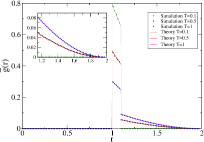
Figure 2: Pair distribution function curves for $N=2$ and $\rho=0.5$ for different temperatures. A clear agreement between theoretical and simulation results is observed. The inset shows same curves on the range $r\in\left[1.15,1.97\right]$.

We present firstly the results for the $N=2$ system, from which exact theoretical results are available.Urrutia and Castelletti (2011b) This allows to make a direct comparison between exact predictions and simulation results. By getting a perfect matching, we ensure that we have solid framework to analyze the few-particle systems of higher $N$. It is also useful for validating the simulation program and thermostating procedure. The pair distribution function is shown in Fig. 2 for different temperatures. A clean superposition between theory and simulation is easily appreciable. For $N=2$ the analytic form of $\bar{g}(r)$ is

$$\bar{g}(r)=Ce_{12}(r)\left[(2R_{\textrm{eff}}-r)^{2}(r+4R_{\textrm{eff}})\right],$$ (21)

with $e_{12}(r)=e^{-\beta\phi(r)}$ and $C=\frac{\pi}{12Z_{2}}$.Urrutia and Castelletti (2011b) First, the null values in the range $0<r<1$ is a trivial effect of the hard core repulsion. Then in the range $1<r<1.1$ there is always a main peak. This peak is an expected result, given the shape and length of the potential: inside the well attractive zone, particles are more likely to be closer. Another common element of these curves is the presence of “tails”, i.e. the smooth monotonically decreasing segments that are seen for ranges of $r$ beyond the main peak. The tail ends at $2R_{\textrm{eff}}=1.97$ (cavity diameter) which is the maximum possible pair distance. Since there is not particle interaction for pair distance over $1.1$, the tail is proportional to the probability of finding a pair of hard spheres in spherical confinement at a given distance. The relation between the main peak and the tail sizes is driven by the temperature: a steep jump in $e_{12}$ will happen at low $T$, and $e_{12}$ approaches to unity at high $T$. From a phenomenological standpoint, at low $T$ the particles lack the energy to escape from the well, thus forming a permanent short ranged bond. At high $T$, the kinetic energy is far greater than the well depth, meaning that the system resembles one of colliding hard cores (HS limit). For higher $N$, the competition between the structure (peaks) and the tail (no interaction) is one of the most visible effects when increasing $T$. The relation between $\bar{g}_{\textrm{sw}}(r)$ and $\bar{g}_{\textrm{AO}}(r)$ was not studied before, at the best of our knowledge. However, based on our analysis of the case $N=2$, we propose that the corresponding functions are $\bar{g}_{\textrm{sw}}(r)/e_{12}^{(\textrm{sw})}(r)$ and $\bar{g}_{\textrm{AO}}(r)/e_{12}^{(\textrm{AO})}(r)$, with $r>1$. This mapping produces small changes in the shape of the main peak of $\bar{g}_{\textrm{AO}}(r)$ in comparison with $\bar{g}_{\textrm{sw}}(r)$.

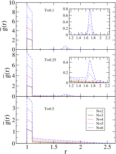
Figure 3: $\bar{g}(r)$ curves for $N=2$ to $6$ at fixed number density $\rho=0.5$. Chosen temperatures are (top to bottom in order) $0.1$, $0.25$ and $0.5$. The insets present the second neighbour peak in more detail.

As can be seen in Fig. 3, where it is shown the pair distribution function for 3 to 6 particles inside the cavity, adding particles to such a small system will necessarily cause qualitative changes beyond the two-body analysis. Nonetheless, certain core aspects remain the same: those that are linked to the potential shape (main peak and HS limit). Since the integral over the complete space of $\bar{g}(r)$ is $N(N-1)/2$,Urrutia and Castelletti (2011b) it is expected that lower $N$ (at fixed $\rho$) show overall lower curves. Also, $R_{\textrm{eff}}=\left(3N/4\pi\rho\right)^{1/3}$ means that at low $N$ values and fixed number density, cavity size is highly susceptible to add or subtract a single particle. The shape of $\bar{g}(r)$ for different temperatures can be used to provide qualitative aspects of the morphology of the clusters. For very low temperatures ($T<0.1$) the particles form a rigid cluster minimizing the overall system energy. Every close neighbor ($1<r<1.1$) adds up $-\varepsilon$ to the potential energy. The bonds are mainly permanent, meaning stable pair distances leading to clearly discernible peaks.

For these small systems, it is possible to interpret the low $T$ curves $\bar{g}(r)$ just by considering the clusters shapes. Three particles form a triangle and four a regular tetrahedron, both of which have in common that all the particles are first neighbors between themselves. This means that the whole probability of finding a pair at certain distance will localize in the first neighbor range of the pair distribution function (main peak). This isolated peak is shown for $N=2,\,3$ and $4$ in Fig. 3, top panel.

The shape of $\bar{g}(r)$ for $N=5$ can be understood starting from the $N=4$ regular tetrahedron and then adding an extra particle on one of its faces. The result is an hexahedron composed of two regular tetrahedrons in contact by one face. The resulting structure has three particles, each one with four first neighbors and two particles with three first neighbors and one second neighbor. A cluster geometry with second neighbors gives rise to a non vanishing probability of finding a pair distance larger than the main peak region. The stable structure with the second neighbor distance in a constrained region results in a second peak.

For the case $N=6$ there are two observed cluster geometries. One of them is the regular octahedron. However, the most frequent geometry observed in the simulations is an irregular octahedron. This irregular polyhedron has a typical path of formation starting from a hexahedral cluster of five particles to which the remaining particle adds over one of its faces. For extremely low temperatures ($T\ll 0.1$), once the particles form their bonds, they will stay bonded permanently. For a softer cluster ($T\lesssim 0.1$), single bonds have a slight chance of breaking and a rearranging of the cluster structure can take place. The secondary peak of $\bar{g}(r)$ is sensitive to these different structures as shown in the inset of the top panel in Fig. 3. There are two secondary peaks both related with second neighbor distance: the larger one represents the second neighbors in the irregular octahedron while the smaller one is characteristic of the regular body. The significant height difference shows that the irregular cluster is more frequent over time. We point out also that both geometries have the same number of first neighbors being thus isoenergetic. Therefore, from a statistical mechanics point of view, the only factor that can lead to the prevalence of one geometry over the other is strictly coming from entropic contributions. The irregular cluster presents lower symmetry and higher entropy.

Increasing the temperature leads to the break up of multiple bonds, which results in flexible or plastic clusters. For intermediate $T$ ranges ($0.1<T<0.25$), the particles remain constantly linked, but now they are not tightly bound. Certain bonds are likely to break, enabling the particles to displace inside the cluster. The inset of Fig. 3 for $T=0.25$, shows that the isolated peaks are surrounded by non-vanishing values. For example, the triangle for $N=3$ breaks one of its pair bonds in such a way that it opens up and stretches like a chain. For higher $N$, is essentially the same. Additional translational freedom leads to possible deformations into wider shapes than the original rigid body. The weaker the structure is, the lower the main and second peak become, favoring pair distance probability on the surrounding areas.

For higher temperatures, ($T>0.3$) soft cluster starts to dissociate and single particles are free to have any distance from the cluster, inside the cavity limits. Any kind of stable structure fades out and only instantaneous pairs endure. As can be seen in the bottom panel of Fig. 3, the tail engulfs any close range structure and the main peak reduces around half of its height, compared to the $T=0.25$ panel. Higher temperatures do not add any qualitative variation: the main peak will decrease until it becomes part of the tail, in the HS limit.

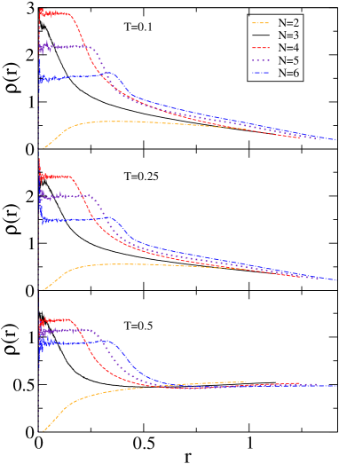
Figure 4: Density profiles for $N=2$ to $6$ at fixed number density $\rho=0.5$. The chosen temperatures are (top to bottom in order) $0.1$, $0.25$ and $0.5$.

Density profiles, shown in Fig. 4, present very explicitly the inhomegeneity of the system. Unlike commonly studied bulk systems, there are significant local spatial variations of the one body density function. Note that $R_{\textrm{eff}}$ varies with $N$, in Fig. 4. It takes values from $R_{\textrm{eff}}=1$ for two particles to $R_{\textrm{eff}}=1.9$ for six particles. For the case $N=2$ the density vanishes in the center because if one particle in placed at $r\approx 0$, the available volume for the other one becomes very small. For density values that define effective radii higher than the particle diameter, i.e. $N=3$ to $6$, all the profiles have similar form, independently of particle number. The profiles have two distinct regions. An approximately constant density on the center of the cavity, that is cut at the vicinity of the wall ($R_{\textrm{eff}}-r<1$) and the "interfacial" region closer to the wall. The extension of the plateau depends on the relation of cavity size and particle diameter, as observed from the different sizes at equal number density in Fig. 4. For low temperatures the system may be treated as a single nearly-rigid body, free to translate and rotate in the central region. When the cluster gets closer to the wall, some possible cluster orientations are restricted, leading to a reduction in rotational entropy. Consequently, it is more likely to find the cluster in the central region. Higher temperatures soften the particles’ bonds progressively, causing a reduction of the disparity between the plateau and the region close to the wall. Once dissociation becomes dominant for high temperatures, depletion arises and the wall starts to have a more intense effective attraction. Further increase in the temperature makes the wall attraction higher, while the particle correlation disappears. At the HS limit the highest probability of finding a particle is at the wall. This was also observed in a system of pure HS particles in spherical confinement.Urrutia and Pastorino (2014) For the AO system we expect similar density profiles to those of SW for equivalent temperature and packing fraction. The temperatures $T=0.1$, $0.25$ and $0.5$ correspond to (top to bottom panels in Fig. 4) polymers inverse packing fraction $\eta_{p}^{-1}=0.694$, $1.50$ and $2.84$, respectively. As we will see, the case $T=0.1$, may be a too small temperature to use the extended law of corresponding states.

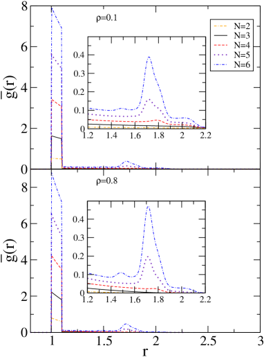
Figure 5: $\bar{g}(r)$ curves for $N=2$ to $6$ at fixed temperature $T=0.25$. Number densities are $0.1$ (Top) and $0.8$ (Bottom). The insets present the second neighbour peak in more detail.

The structure dependency on $\rho$ is far more subtle than on $T$. In Fig. 5 curves of $\bar{g}(r)$ at $T=0.25$ and for two different densities are shown. One observes that the shape of the peaks remain practically unaltered. Global values of the curve raise for higher number densities, because the normalization is the same in a smaller cavity size. We have shown the case $T=0.25$, as an example but we observed the same general picture for other values of $T$ which are not presented here.

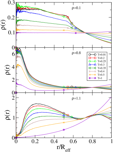
Figure 6: Density profiles for $N=5$ at different temperatures. Number densities are $0.1$ (Top), $0.8$ (Center) and $1.1$ (Bottom).

From here on, we select the case $N=5$ to give more detailed analysis. This case is the only one that presents a second peak but does not have multiple stable geometries, as the case $N=6$. At low temperatures it is observed a clearly defined structure, while retaining little longer range order. The $N=5$ results can be extrapolated to the other few-particle systems. Density profiles are shown in Fig. 6 for a wide range of temperatures and number densities. As already pointed out, at low and intermediate densities there exist a plateau and an interfacial region close to the wall. Increasing the temperature leads to an overall probability density favoring position closer to the wall, as a result of relatively stronger depletion attraction.Urrutia and Pastorino (2014); Israelachvili (2011) The higher the density, the smaller the available free volume for the rigid cluster, thus the plateau becomes smaller and steeper. At certain number density there is no more room to locate a particle in the center of the cavity. The available space is so small that a particle at the center would push the remaining ones out of bounds. This is shown in the lower panel of Fig. 6, which exhibits an excluded volume region close to the center of the cavity. This gives a clear insight of how, at high densities, the system conformation and translation becomes dominated by the cavity shape. At high densities, rigid clusters have low translational freedom and therefore their constituent particles stand at approximately fixed distances from the center. Cluster structure gets expressed on the density profiles that show local maxima and minima. Increasing the temperature softens the cluster, causing the local structure features to disappear, leaning towards monotonous curves. Finally, at dissociation temperatures, the depletion dominance gets clear and the density at the wall is the highest in the profile. We note here a difficulty, intrinsically related with the spherical shape of the cavity. The local properties are hard to measure in the central region because it is poorly sampled. Indeed, the sampling becomes poorer as $r$ decreases towards the center of the pore. This effect is produced by the rapid reduction of the sampled volume that produce large fluctuations in $\rho(r)$ and other quantities. These fluctuations can also be observed in Fig. 4.

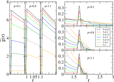
Figure 7: $\bar{g}(r)$ for $N=5$ at different temperatures and representative number densities. Left panel: detail of the main peak, right panel: detail of the second peak for $r\in\left[1.15;3\right]$.

In Figure 7 a similar systematic approach is applied for the $\bar{g}(r)$ curves under density variation. Each studied density $\rho=0.1$, $0.8$ and $1.1$ corresponds to a cavity diameter of $4.57$, $2.28$ and $2.05$, respectively. By increasing the temperature, pair bonds are more likely to break and produce dissociations. The odds of a separated pair to become together again is smaller at larger free space. As a consequence, main peaks fall more abruptly at dissociation temperatures and lower densities. At high densities, there is not enough room for the particles to stay away from each other, which forces an increase in the probability of finding pair separations inside the well range, even if particles have a very high kinetic energy, as compared to the well interaction energy $\varepsilon$. At $\rho=1.1$ it is noticeable how cavity diameter is close to second neighbor distance. For $N=5$ the rigid cluster geometry is also the most compact the system can achieve, the cavity is only a slightly larger than the smallest possible configuration. This implies that the cluster as a whole is practically locked in the center, allowed mostly only to rotate. As already observed in Figure 6, at high densities and low temperatures, the particles of the rotating rigid body maintain a stable distance from the center. For $\rho>1.1$, the wall cavity squeezes the system, shortening the second neighbor distance.

Despite the SW interaction is isoenergetic once inside the field range, the main peak of $\bar{g}(r)$ shows a negative slope as can be observed in Figs. 2, 3, 5 and 7. This implies that, within the interaction range $r\in\left[1,1+\lambda\right]$, particles tend to be at closest distance instead of near the external side of the well. Theoretical results for $N=2$ (Eq. 21) points out that the slope originates from the particle-cavity interaction. Basically the main peak is an offset mounted on a decreasing function. This can be rationalized by noting that a closer pair has more free space in the cavity than a stretched one, increasing the traslational entropy. Also particle collisions with a curved concave wall will, in average, tend to group them together.

IV.2 Thermodynamic quantities

We focus on four thermodynamic properties to characterize the system as a whole. We analyze the pressure and the energy of the system, that have robust definitions and are measured in a straightforward way. Additionally, we study the surface tension and the surface adsorption, which are intrinsically related with the inhomogeneous nature of the system. These last quantities are more subtle and difficult to measure by simulation.

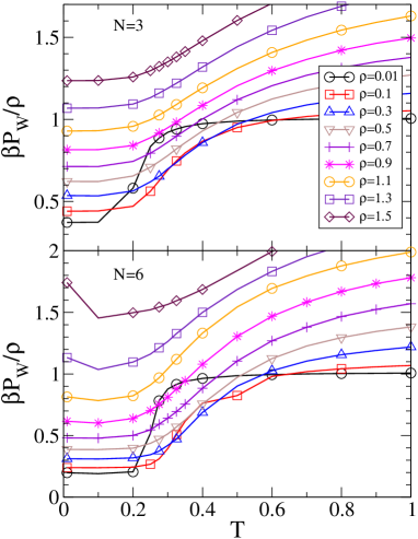
Figure 8: Compressibility factor $\beta P_{w}/\rho$ as a function of temperature, for different number densities for $N=3$ (Top panel) and $N=6$ (Bottom panel).

Pressure on the wall is expected to increase with temperature and number density, given that both parameters should increase the average number of collisions on the wall. We work with the compresibility factor $\beta P_{w}/\rho$ in Fig. 8 to eliminate the linear dependence, allowing to distinguish deviations from the ideal case $\beta P_{w}/\rho=1$. Only the high temperature and very low density cases follow the ideal behavior, when the relative well attraction is too weak and excluded volume from the cores is negligible. Cluster to dissociation temperatures are mediated by a sudden increase in $\beta P_{w}/\rho$ and further saturation. The jump becomes smoother for higher densities as a result of what has been pointed out from $\bar{g}(r)$ analysis: with less space for separation, qualitative differences between a cluster and unbounded particles are smaller. The mentioned depletion emergence, for any density value at high $T$, explains the asymptotic increase of $\beta P_{w}/\rho$ until the HS limit.

At very low temperatures, the system is far away from the ideal gas behavior because the relative potential well produces a cluster. In this limit the system compressibility factor increases monotonically for increasing density. We attribute this to the behavior of a unique finite-size cluster allowed to stay in an effective volume $V_{\textrm{cluster}}<V$. The single cluster behaves as an ideal gas, and thus, its compressibility factor is $\beta PV_{\textrm{cluster}}=1$ i.e. $\beta P/\rho\simeq N^{-1}V/V_{\textrm{cluster}}$. This explains the low-density and low-temperature values $\beta P_{w}/\rho\gtrsim 0.33$ and $\beta P_{w}/\rho\gtrsim 0.17$ for $N=3$ and $6$ respectively. At intermediates temperatures, when the bond-breaking probability is non-negligible, the case of low density raises much more rapidly to its saturation value than those of higher densities. This could be related to the strong reduction of recombination rate at lower densities. Once a bond is broken the probability of the particles to meet again is very small. This is not the case for intermediate to high densities.

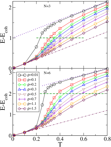
Figure 9: $E-E_{\textrm{coh}}$ as a function of $T$ for different number densities Top panel shows $N=3$ and Bottom panel $N=6$ cases. The horizontal dashed line plots $\left|E_{\textrm{coh}}\right|=-E_{\textrm{coh}}$.

The mean energy per particle $E$ is the addition of the kinetic term $3T/2$ driven by the temperature and the mean potential energy. For low temperatures, where $\left|\phi_{N}\right|/N\gg 3T/2$, the system is in a rigid cluster state. Then, $E$ can be precisely calculated as the number of bonded pairs for a given geometry. We call that value cohesion energy $E_{\textrm{coh}}$, which is the lowest (fundamental) possible energy of the system and we define it as the zero value in Fig. 9, presenting the energy versus temperature. Average energy per particle has a similar behavior to the one of the pressure in Fig. 8. For low density, it presents an abrupt increment in going from low to higher temperatures ($T\sim 0.2$). This jump agrees with the range of non-rigid cluster, ending at dissociation temperatures ($T\sim 0.3$). Then it follows a weak linear variation for high temperatures, according to the equipartition theorem. It is worth noting that for systems with a unique stable rigid cluster geometry at low temperatures, all the curves must collapse to a single with slope $3/2$, independently of the density. For reference, the behavior of both, the pure kinetic energy and the shifted one (plus $\left|E_{\textrm{coh}}\right|$), are also shown in dotted and dot-dashed lines in Fig. 9. Rigid clusters constitute compact structures, and increasing the density does not changes the number of first neighbors. Higher density lines have lower values because the particles are closer, so SW interactions are forced. The changes produced with increasing temperature in each curve are more pronounced for higher $N$, because the rigid cluster has more bounds (per particle) to be broken. This feature is also shown for the different values that takes $\left|E_{\textrm{coh}}\right|$, in dashed line. The line also serves to visualize the condition $E=0$, which characterize the equilibrium between potential and kinetic energies. This crossover line separates two characteristic regions: one where the potential energy dominates over the kinetic energy, proper of clusters, and another one where kinetic energy dominates, a feature proper of gases.

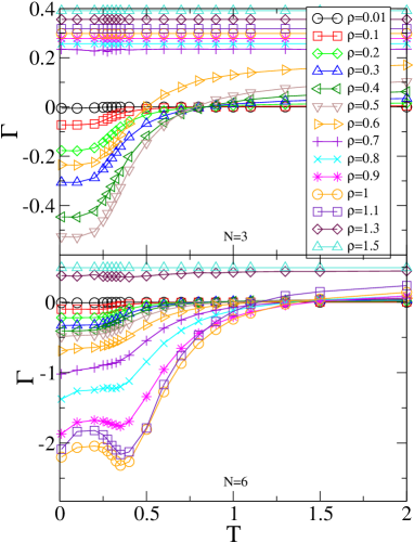
Figure 10: Adsorption $\Gamma$ as a function of temperature for different number densities. The cases $N=3$ (Top panel) and $N=6$ (Bottom panel) are shown.

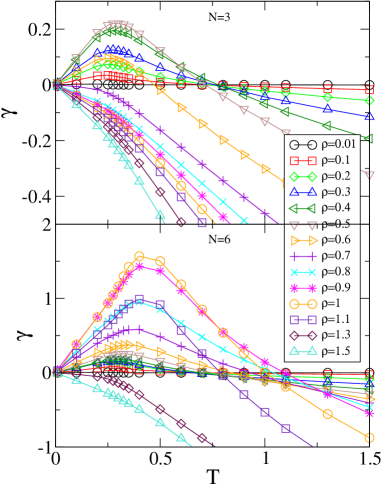
Figure 11: Surface tension as a function of $T$ for different number densities. The cases $N=3$ (Top panel) and $N=6$ (Bottom panel) are shown.

Surface adsorption $\Gamma$ and surface tension $\gamma$ are basic properties used to characterize the inhomegeneity induced on the system by the presence of walls. They are measured in the same way as a in a previous work.Urrutia and Pastorino (2014) We won’t delve into details and only give here the definition of $\Gamma$, and the expression of $\gamma$, based on Laplace equation: $\Gamma=\left(\rho-\rho_{c}\right)\frac{V}{A}$ and $\gamma=\frac{P_{c}-P_{w}}{2}R_{\textrm{eff}}$. Here $\rho_{c}$ ($P_{c}$) refers to the average density (pressure) near the center of the cavity. These magnitudes are difficult to measure because one must fix a criterion to choose the region where averages should be done. The criterion must be applied for all the available range of $\rho$ and $T$. Note that at large $R_{\textrm{eff}}$, the density profiles attain a nearly constant value in the central region (plateau). At constant $N$, the density $\rho_{c}$ becomes higher for smaller cavity radius until a limiting value, in which particles cannot freely place themselves in the center. This central region progressively turns into an excluded zone. It is important to note that at such high packing values, the definition of $\rho_{c}$ is less accurate, since there is not a clear distinction between the center region and that in the vicinity of the wall. Adsorption is shown in Fig. 10. For low densities, adsorption is negative for small $T$ and then experiences a jump around dissociation temperatures to flatten at higher values of $T$. It becomes positive at high temperatures. For high densities, adsorption is positive and nearly independent of the temperature. The limiting cases of temperature are clearly identified. For high temperature $\Gamma$ is positive and increase monotonously with density. In the case of low temperature, for small densities $\Gamma$ is negative and decreases with increasing $\rho$, up to a certain minimum value. Further increment of $\rho$ produces a sudden rise of $\Gamma$, that becomes positive. This behavior goes in line with that observed in the density profiles, in Section IV.1. $\rho(r)$ presents an enhancement close to the wall for $\Gamma>0$ and an increment in the center for $\Gamma<0$.

Fig. 11 shows the surface tension $\gamma$ for three (Top panel) and six particles (Bottom panel). At vanishing temperature they start from 0, having then two distinctive behaviors. For low to intermediate densities the $\gamma$ curves are positive at low $T$. They start with positive slope, reach a maximum value, to become negative at high temperatures. For high densities, $\gamma$ curves are negative. They start with negative slope and decrease monotonously with temperature.

The two different characteristics of $\gamma$ can be rationalized by considering that when clusters are favored at medium to low densities, the system tends to get far from the cavity wall, having the cluster size as its characteristic size. This minimizes the intrinsic area of the system, going along with a negative adsorption and an increase of density at the center of the cavity. At high enough temperatures, the system behaves as HS particles, having the confining cavity as a characteristic size, with an effective entropic attraction from the wall, and a negative surface tension.Urrutia and Pastorino (2014) The curve that shows the global maximum of surface tension corresponds to higher density for $N=6$ than for $N=3$. Also, the temperature of those global maxima of $\gamma$ is shifted towards higher values.

The approximate linear dependence of $\gamma$ with $T$ for both very low and high temperatures is explained by the expected hard sphere limit where $\beta\gamma$ only depends on density. The behavior upon variation of density is similar to that observed for $\Gamma$.

Some of the measured thermodynamic properties of the SW system can be readily mapped to the AO model by the established relation between $T$ and $\eta_{p}$. We expect one of these magnitudes to be the pressure on the wall, once the energy scale is compensated [as in the case of $\beta\phi_{\textrm{AO}}$ in Eq. (9)], thus $\beta P_{w}$ but also $\beta P_{w}/\rho$ that was plotted in Fig. 8 could be mapped. The measured surface tension is similar to the pressure, it should be transformed to $\beta\gamma$. A third magnitude is $\Gamma$ which does not scales with $T$ and depends on characteristic features of $\rho(r)$. The case of energy is more complicated because in the AO system the energy is purely kinetic, and therefore the energy can not be mapped.

IV.3 Phase diagrams

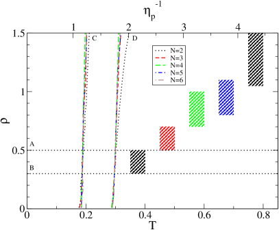
Figure 12: Superimposed phase diagram for $N=2$ to $6$. Vertical lines come from analyzing the pair distribution function. At the left side of C, there is a hard cluster region. Between C and D we define a soft or plastic cluster region and at the right side of C dissociation starts to happen. Horizontal lines show density points where density profiles are maximum (B), or vanish at the center (A). The rectangles show the range of $\rho$ between A and B positions for every $N$.

In Fig. 12 we show the change of the main characteristics of the phase diagram with the variation of $N$. This summarizes variation of structural properties with $T$ and $\rho$. The vertical lines come from the analysis of the pair distribution function, by comparing the height of the main peak $\bar{g}(r=1^{+})$ with that in the region next to the main peak $\bar{g}(r=1.1^{+})$, and its connection with the qualitative behavior of the system, obtained by direct visualization of the dynamics of the particles. C corresponds to $\bar{g}(r=1.1^{+})/\bar{g}(r=1^{+})=0.005$ and D to $\bar{g}(r=1.1^{+})/\bar{g}(r=1^{+})=0.03$. The relations between those points have been picked by noting that those values match cluster softening (C) and dissociation process (D). These lines divide temperature domains by particle conformation: low temperatures until C mostly defined by particles gathering in a hard cluster. Between C and D the system forms a soft cluster with relative movements among particles. For higher temperatures, beyond D, frequent dissociations are observed. The horizontal lines come from the analysis of the main features of the density distribution. Line A indicates the cases in which the density profile at the center of the cavity $\rho(r=0)$ reaches its maximum, and line B when it becomes zero [$\rho(r=0)=0$]. The former case represents low translational freedom for the particle that is at the center, while for the later there is such a high density (or a small cavity), that a particle can not be in the center due to the excluded volume. These horizontal lines delimit the following regions: below B there is a zone in which the system is moderately inhomogeneous. The region limited by A and B corresponds to a strong reduction of freedom of motion that reduces the occupation in the center. For densities beyond line A the center of the cavity is an excluded volume (high confinement). Note that a third horizontal line (not shown) fix the maximum density of the confined system where it becomes completely caged. This density can be calculated with a simple geometrical approach and varies with $N$. In contrast to the vertical lines, the position of A and B are strongly dependent on $N$.

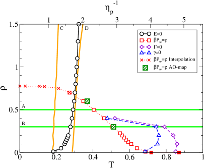
Figure 13: Phase diagram for $N=2$ with characteristic curves. A, B, C and D thick lines are the same from Fig.12. Additionally, curves indicating $E=0$ (black circles), $\beta P_{w}=\rho$ (open red squares); $\Gamma=0$ (green diamonds), and $\gamma=0$ (blue triangles) are shown. Red crosses present the values obtained by interpolating the curves of $\beta P_{w}/\rho$ for specific density values. These lie between points for which simulation results are available thus allowing to complete the curve at the saturation area. The two red filled squares show exact analytic values for $\beta P_{w}=\rho$ and $\Gamma=0$ at $\rho\rightarrow 0$. Green bigger squares represent the AO model results for $\beta P_{w}=\rho$. In the top x-axis the scale of packing fraction of polymers in the AO model is presented.

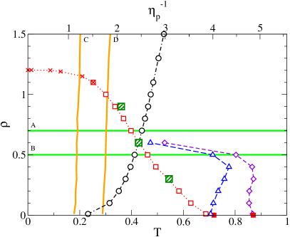
Figure 14: Phase diagram for $N=3$ with characteristic curves. Symbols, lines and top x-axis follow the same notation from those of Fig.13.

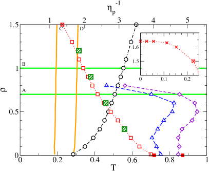
Figure 15: Phase diagram for $N=4$ with characteristic curves. Symbols, lines and top x-axis follow the same notation from those of Fig.13. The inset shows details of $\beta P_{w}=\rho$ at low temperatures.

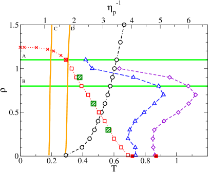
Figure 16: Phase diagram for $N=5$ with characteristic curves. Symbols, lines and top x-axis follow are the same notation of those of Fig.13.

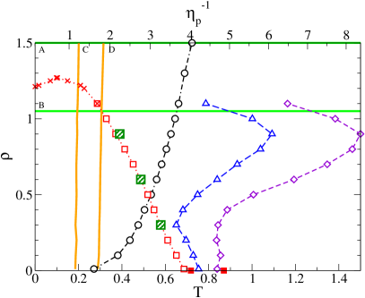
Figure 17: Phase diagram for $N=6$ with characteristic curves. Symbols, lines and top x-axis follow the notation of Fig.13.

In Figs. 13 to 17 we present the phase diagram for the different number of particles studied. It is shown a set of characteristic values of density and temperature labeled with letter A, B, C and D. They separate regions where the systems present different qualitative behavior. These regions would represent different phases of the system in a macroscopic context.

Additionally, the scalars chosen to distinguish different qualitative behavior of the system are the $(T,\rho)$ points on which: kinetic energy is equal to potential energy (black circles), pressure on the wall follows ideal gas equation of state (red open squares and crosses), adsorption and surface tension change their signs (green diamonds and blue triangles, respectively). We point out that the $(T,\rho)$ grid step is $0.1$, except for the cases of low temperatures (e.g. $T=0.01$) and higher densities where the steps become more spaced. In particular, low temperature $\beta P_{w}=\rho$ points (red crosses) have been attained by interpolating $\beta P_{w}$ curves for specific density values, whose variations are too small for our scale.

The $E=0$ curve (open circles) divides the phase space. Towards the left, the (modulus of) potential energy is higher than the kinetic energy and the opposite case is true, towards the right. In the region with $E<0$ (at the left of $E=0$) the potential energy dominates. This feature is characteristic of systems that spontaneously collapse in cluster aggregates or condensed phases, but also of cold enough compressed systems, where the available space is reduced. On the opposite, when $E>0$ (at the right of $E=0$ curve) the kinetic energy dominates and this is typical of systems of free particles, as the case of diluted gases. Note that this last region includes a high enough temperature and high density range, where particles stay together, as a consequence of the strong confinement. The $E=0$ curve is specially sensitive to changes in $N$, since it is affected by the average number of bonds per particle. At low $N$, adding particles increases the maximum number of bonds per particle, given that the system is too far away from bulk case. As a result of this, the curve shifts towards higher temperatures upon increasing $N$. This is specially observed comparing Figures 13 and 14. The curve flattens for higher densities since smaller cavity forces bond formation, leading to a fixed potential energy value of a tightly packed cluster. This curve has not a counterpart for the colloid-polymer mixture analyzed with the AO model. Even when there is an effective potential between colloids, the system is athermal and the origin of the potential is purely entropic. Both, colloids and polymers have only kinetic energy, thus $E\neq 0$ for non zero temperatures.

The curve $\beta P_{w}=\rho$ (open squares) indicates the points of the $(T,\rho)$ where the EOS for the system pressure behaves like the ideal gas pressure $P_{\textrm{id}}$. At the left side and below of the $\beta P_{w}=\rho$ curve, $P_{w}<P_{\textrm{id}}$, the system is undercompressed with respect to the ideal gas (at the same temperature and number density). This region encloses the origin. Outside this region $P_{w}>P_{\textrm{id}}$ the system is overcompressed in comparison with the ideal gas. For low densities and high temperatures this is expected as a consequence that depletion favors wall contact. Higher densities force wall contact, independently of temperature. The theoretical prediction based on the limit of large $V$ (low density) is shown with a red square on $T$ axis. Notably, the obtained limiting temperature fits the curve and is independent of $N$. From $N=3$ to $6$ all these curves follow a similar behavior: from zero density up to $\rho\approx 1$, where $T\approx 0.3$. The curves at lower temperatures show a strong dependence with $N$. It is interesting to note that the critical temperature of the vapor-liquid metastable transition in the studied short-range SW system is $T=0.47$, which, for the largest values of $N$, nearly coincides with the intersection of zero-energy and ideal gas pressure curves.

The $\beta P_{w}=\rho$ curve was selected to verify the validity of the corresponding-states mapping between SW and AO in confined systems. Using Metropolis-Rosembluth Monte Carlo calculationsMetropolis et al. (1953); Rosenbluth and Rosenbluth (1954) we have evaluated the density distribution of the AO system (for few values of $\rho$), and used the contact theorem Eq. (11) to evaluate $\beta P_{w}$. Thus, we seek for the value of $\eta_{p}$ that produce $\beta P_{w}=\rho$. Extended corresponding state law [see Eq. (14)] was used to evaluate the temperature of the corresponding SW equivalent system. Calculated values are drawn in green squares at Figs. 13 to 17. The obtained values of $\eta_{p}^{-1}$ are given at the top horizontal x axis, while the equivalent temperature of the SW system can be read at the bottom axis. We found a general coincidence between Monte Carlo results for AO and simulation results for SW, along all the analyzed range. At lower temperatures, near clusterization, the mapping between both systems becomes poorer. This is expected, because the use of the extended law of corresponding states is not documented for freezing temperatures.

Zero surface adsorption and surface tension curves indicate where there is no excess in surface of particle concentration or free energy, respectively. As it was mentioned in Sec. IV.2, both are difficult to measure. $\Gamma$ and $\gamma$ reveal a strong reduction of accuracy at very low density where the system is quasi-homogeneous and both quantities become very small. This makes specially hard to measure the value of $T$ at which $\varGamma=0$ and $\gamma=0$ for $\rho\rightarrow 0$. In addition, given that $\Gamma$ and $\gamma$ become ill defined at high densities we do not evaluate zero surface excess in this case. In summary, the results presented here give a general idea of the position and shape of both curves in the $(T,\rho)$ plane. Adsorption illustrates the relation between the density of particles at the center of the cavity and those closer to the wall. Towards the left side, where $\Gamma<0$, the particles are more likely to be at the center of the cavity. For $\Gamma>0$, at the right side, particles favor positions close to the wall.

V Conclusions

In this work we studied thoroughly the properties of few colloidal particles confined in a spherical cavity. We adopt the short-range square well model and provide a deep characterization of the structural and thermal properties of systems of 2, 3, 4, 5 and 6 particles in a spherical pore for the complete relevant ranges of density and temperature. Additionally, we compare the simulations with exact results for the case $N=2$. Applying an extension of the corresponding states law to confined systems, we establish a mapping between the square well system and the AO model for effective interactions between colloids in a polymer colloid mixture. We also developed the statistical mechanical approach to systems of few particles, SW and AO, in confinement and map the pressure on the wall at a given temperature in the SW system to the equivalent packing fraction of polymers in the AO system.

The structure of the system ranging from low density to almost caging of the particles in the cavity was characterized through the pair correlation function and density profiles for the entire relevant range of temperatures. Thermal bulk properties such as energy and pressure on the wall were calculated and characterized. Different effects of confinement were also studied, identifying their energetic or entropic origin and focusing on the inhomogeneities present in the system. Surface properties were analyzed with quantities reminiscent of surface tension and adsorption in macroscopic counterparts of the square well system.

We characterized the morphology of these systems, defining different regions of similar behavior and criteria to provide phase diagrams in the $(T,\rho)$ plane, for the different number of particles. In this phase diagram, we identified temperature regions where the system behaves as a rigid cluster, as a plastic cluster, and a region where the system dissociates, up to the limit of hard-sphere-like behavior at very high temperatures. In the density domain, we recognized regions with different degrees of inhomogeneity which can be classified in the following categories: low-to-moderate, moderate to excluded volume, and excluded-volume to caging regions. We defined several characteristic curves in the phase diagram, such as that of zero energy, ideal gas pressure, zero adsorption and zero surface tension. These lines delimit meaningful references in the phase diagram, that were used as a complement for the analysis.

Appendix A Effective potential and AO partition function

We show here how to transform Eq. (7) in Eq. (8). To this end, we analyze the term $\sum_{N_{p}}\frac{z_{p}^{N_{p}}}{N_{p}!}Z_{N,N_{p}}$ in Eq. (7), where the (canonical ensemble) colloid-polymer mixture CI reads

$$Z_{N,N_{p}}=\int_{V^{N}}\int_{V_{p}^{Np}}e^{-\beta\left(\phi_{cc}+\phi_{cp}\right)}d\mathbf{r}_{p}^{N_{p}}d\mathbf{r}_{c}^{N}\>,$$ (22)

with $\phi_{cc}=\sum_{i,j}\phi_{ij}^{(cc)}$, $\phi_{cp}=\sum_{i}^{(c)}\sum_{k}^{(p)}\phi_{ik}^{(cp)}$. $\phi_{ij}^{(cc)}$, $\phi_{ik}^{(cp)}$ are the spherically symmetric pair potentials. Note that the region $\mathcal{C}$ where the center of colloids are confined (with volume $V$) is different to the region $\mathcal{P}$ where the center of polymers lies (with volume $V_{p}$). In fact, the boundary of $\mathcal{P}$ must be placed in a region where the polymers reach their bulk properties. For the AO system with $q<0.1547$ confined in a spherical pore, the smallest region $\mathcal{P}$ is an sphere with radius $R_{0}+\sigma_{p}/2$.

Polymers behave as ideal gas particles. If we fix the position of the colloids, they exert a fixed external potential to the polymers and thus

$$\int_{V_{p}^{Np}}e^{-\beta\phi_{cp}}d\mathbf{r}_{p}^{N_{p}}=\biggl{(}\int_{V_{p}}e^{-\beta\phi_{cp}}d\mathbf{r}_{p}\biggr{)}^{N_{p}}=Z_{\otimes}^{N_{p}}\>,$$ (23)

where $Z_{\otimes}$ is the CI of one polymer in $V_{p}$ at fixed colloids. Furthermore,

$$\sum_{N_{p}}\frac{z_{p}^{N_{p}}}{N_{p}!}Z_{N,N_{p}} = \int_{V^{N}}e^{-\beta\phi_{cc}}\sum_{N_{p}}\frac{z_{p}^{N_{p}}}{N_{p}!}Z_{\otimes}^{N_{p}}d\mathbf{r}_{c}^{N}\>,$$ (24)

$$= \int_{V^{N}}e^{\bigl{(}-\beta\phi_{cc}+z_{p}Z_{\otimes}\bigr{)}}d\mathbf{r}_{c}^{N}\>,$$ (25)

and thus we can simply analyze the case of one polymer. We introduce the Mayer function for the colloid/polymer Boltzmann statistical weight $e_{i}=\exp\bigl{(}-\beta\phi_{i1}^{(cp)}\bigr{)}=1+f_{i}$ in $Z_{\otimes}$ to obtain

$$Z_{\otimes}=\int_{V_{p}}\Bigl{(}1+\sum_{i}f_{i}+\sum_{<ij>}f_{i}f_{j}+\ldots\Bigr{)}d\mathbf{r}_{p}\>,$$ (26)

where higher order terms are products of three or more functions $f$ concerning the position of three or more colloids. In this integrand $f_{i}$ is minus one for $\mathbf{r}_{p}$ such that the (center-to-center) $i$th-colloid to polymer distance fulfills $x_{i}<\sigma+\sigma_{p}$ and otherwise is zero. $f_{i}f_{j}$ is one if $\mathbf{r}_{p}$ fulfills both $x_{i}<\sigma+\sigma_{p}$ and $x_{j}<\sigma+\sigma_{p}$ and is zero otherwise, and so on. Once integrated, $Z_{\otimes}$ takes the form

$$V_{p}-\frac{4\pi}{3}\sigma^{3}\left(1+q\right)^{3}N+\sum_{<ij>}V_{o}\bigl{(}r_{ij}\bigr{)}+\ldots$$ (27)

Here $V_{o}\bigl{(}r_{ij}\bigr{)}$ is the overlap volume between two spheres with radius $\bigl{(}\sigma+\sigma_{p}\bigr{)}/2$ and extra terms include the overlap of at least three spheres. Turning to the integrand of Eq. (25), we utilize the identities $z_{p}=\rho_{p}$ and $z_{p}V_{p}=N_{p}$ to obtain

$$\exp\left(N_{p}-N_{p}^{x}\right)\exp\Bigl{[}-\beta\sum_{<ij>}\phi_{\textrm{HS}}\bigl{(}r_{ij}\bigr{)}+\rho_{p}\sum_{<ij>}V_{o}\bigl{(}r_{ij}\bigr{)}\Bigr{]}\>,$$ (28)

with $N_{p}^{x}=\rho_{p}v_{\textrm{exc}}N$ and $v_{\textrm{exc}}=\frac{4\pi}{3}\sigma^{3}\left(1+q\right)^{3}$. In addition, we neglected higher order terms in Eq. (28). These terms are null if $q<0.1547$. For $q\apprge 0.1547$, including the case $q=0.2$ analyzed in the present work, one expects that three-body contribution will be negligible in comparison with two-body terms. Naturally, $\Xi_{p,h}=\exp N_{p}$ and $\beta\phi_{\textrm{AO}}(r)=\beta\phi_{\textrm{HS}}(r)-\rho_{p}V_{o}(r)$, where $\beta\phi_{\textrm{AO}}(r)$ is the same expression given in Eq. (9). Therefore, Eq. (25) is $Z_{N}^{(\textrm{AO})}$. This demonstrates the equivalence between Eq. (7) and Eq. (8).

The described procedure can be generalized in several ways. It is not restricted to the spherical pore, and thus, it applies to other pore geometries like cylinders, cuboids, slits, single walls, etc. Further extensions include the case of non-free polymers where both, colloids and polymers, are confined, the AO model with $q\apprge 0.1547$, and also other non-AO systems with more general interaction potentials. It can also be readily applied to systems of AO particles in spaces with dimensions other than three (discs and hyper-spheres), with $V_{o}\bigl{(}r\bigr{)}$ taken from Ref.Urrutia and Szybisz (2010).

References

- Wang et al. (2011) T.-T. Wang, F. Chai, C.-G. Wang, L. Li, H.-Y. Liu, L.-Y. Zhang, Z.-M. Su, and Y. Liao, Journal of Colloid and Interface Science 358, 109 (2011).
- Weeks (2012) E. R. Weeks, Science 338, 55 (2012).
- Sacanna et al. (2010) S. Sacanna, W. T. M. Irvine, P. M. Chaikin, and D. J. Pine, Nature 464, 575 (2010).
- Meng et al. (2010) G. Meng, N. Arkus, M. P. Brenner, and V. N. Manoharan, Science 327, 560 (2010).
- Lu et al. (2008) P. J. Lu, E. Zaccarelli, F. Ciulla, A. B. Schofield, F. Sciortino, and D. A. Weitz, Nature 453, 499 (2008).
- Wang et al. (2012) Z. Wang, F. Wang, Y. Peng, Z. Zheng, and Y. Han, Science 338, 87 (2012).
- Aarts, Schmidt, and Lekkerkerker (2004) D. G. A. L. Aarts, M. Schmidt, and H. N. W. Lekkerkerker, Science 304, 847 (2004).
- Anderson and Lekkerkerker (2002) V. J. Anderson and H. N. W. Lekkerkerker, Nature 416, 811 (2002).
- de Hoog et al. (2001) E. H. A. de Hoog, W. K. Kegel, A. van Blaaderen, and H. N. W. Lekkerkerker, Phys. Rev. E 64, 021407 (2001).
- Royall, Poon, and Weeks (2013) C. P. Royall, W. C. K. Poon, and E. R. Weeks, Soft Matter 9, 17 (2013).
- Royall, Louis, and Tanaka (2007) C. P. Royall, A. A. Louis, and H. Tanaka, The Journal of Chemical Physics 127, 044507 (2007).
- Urrutia and Pastorino (2014) I. Urrutia and C. Pastorino, The Journal of Chemical Physics 141, 124905 (2014).
- Urrutia and Castelletti (2012) I. Urrutia and G. Castelletti, The Journal of Chemical Physics 136, 224509 (2012).
- Urrutia (2011) I. Urrutia, The Journal of Chemical Physics 135, 024511 (2011), erratum: ibid. 135(9), 099903 (2011).
- Acedo and Santos (2001) L. Acedo and A. Santos, The Journal of Chemical Physics 115, 2805 (2001).
- Li et al. (2014) L. Li, F. Sun, Z. Chen, L. Wang, and J. Cai, The Journal of Chemical Physics 141, 054905 (2014).
- Rivera-Torres et al. (2013) S. Rivera-Torres, F. del Río, R. Espíndola-Heredia, J. Kolafa, and A. Malijevský, Journal of Molecular Liquids 185, 44 (2013).
- Espíndola-Heredia, Río, and Malijevský (2009) R. Espíndola-Heredia, F. d. Río, and A. Malijevský, The Journal of Chemical Physics 130, 024509 (2009).
- Vortler, Schafer, and Smith (2008) H. L. Vortler, K. Schafer, and W. R. Smith, The Journal of Physical Chemistry B 112, 4656 (2008).
- López-Rendón, Reyes, and Orea (2006) R. López-Rendón, Y. Reyes, and P. Orea, The Journal of Chemical Physics 125, 084508 (2006).
- Kiselev, Ely, and Elliott (2006) S. B. Kiselev, J. F. Ely, and J. R. Elliott, Molecular Physics 104, 2545 (2006).
- Liu, Garde, and Kumar (2005) H. Liu, S. Garde, and S. Kumar, The Journal of Chemical Physics 123, 174505 (2005).
- Khanpour (2011) M. Khanpour, Phys. Rev. E 83, 021203 (2011).
- Hartskeerl (2009) T. Hartskeerl, Crystallization and Glassy Behaviour in Short-range Attractive Square-well Fluids, Ph.D. thesis (2009).
- Neitsch and Klapp (2013) H. Neitsch and S. H. L. Klapp, The Journal of Chemical Physics 138, 064904 (2013).
- Armas-Pérez, Quintana-H, and Chapela (2013) J. C. Armas-Pérez, J. Quintana-H, and G. A. Chapela, The Journal of Chemical Physics 138, 044508 (2013).
- Huang et al. (2010) H. C. Huang, W. W. Chen, J. K. Singh, and S. K. Kwak, The Journal of Chemical Physics 132, 224504 (2010).
- Jana, Singh, and Kwak (2009) S. Jana, J. K. Singh, and S. K. Kwak, The Journal of Chemical Physics 130, 214707 (2009).
- Zhang and Wang (2006) X. Zhang and W. Wang, Phys. Rev. E 74, 062601 (2006).
- Pagan and Gunton (2005) D. L. Pagan and J. D. Gunton, The Journal of Chemical Physics 122, 184515 (2005).
- Urrutia and Castelletti (2011a) I. Urrutia and G. Castelletti, The Journal of Chemical Physics 134, 064508 (2011a).
- Reyes (2012) Y. Reyes, Fluid Phase Equilibria 336, 28 (2012).
- Duda (2009) Y. Duda, The Journal of Chemical Physics 130, 116101 (2009).
- Asakura and Oosawa (1954) S. Asakura and F. Oosawa, The Journal of Chemical Physics 22, 1255 (1954).
- Asakura and Oosawa (1958) S. Asakura and F. Oosawa, Journal of Polymer Science 33, 183 (1958).
- Israelachvili (2011) J. Israelachvili, Intermolecular and surface forces (Academic Press, Burlington, MA, 2011).
- Vrij (1976) A. Vrij, Pure Appl. Chem. 48, 471 (1976).
- Germain and Amokrane (2007) P. Germain and S. Amokrane, Phys. Rev. E 76, 031401 (2007).
- López de Haro et al. (2015) M. López de Haro, C. F. Tejero, A. Santos, S. B. Yuste, G. Fiumara, and F. Saija, The Journal of Chemical Physics 142, 014902 (2015).
- Binder, Virnau, and Statt (2014) K. Binder, P. Virnau, and A. Statt, The Journal of Chemical Physics 141, 140901 (2014).
- Winkler et al. (2013) A. Winkler, A. Statt, P. Virnau, and K. Binder, Phys. Rev. E 87, 032307 (2013).
- Statt et al. (2012) A. Statt, A. Winkler, P. Virnau, and K. Binder, Journal of Physics: Condensed Matter 24, 464122 (2012).
- Noro and Frenkel (2000) M. G. Noro and D. Frenkel, The Journal of Chemical Physics 113, 2941 (2000).
- Valadez-Pérez et al. (2012) N. E. Valadez-Pérez, A. L. Benavides, E. Schöll-Paschinger, and R. Castañeda Priego, The Journal of Chemical Physics 137, 084905 (2012).
- Hansen and McDonald (2006) J.-P. Hansen and I. R. McDonald, Theory of simple liquids, 3rd Edition (Academic Press, Amsterdam, 2006).
- Blokhuis and Kuipers (2007) E. M. Blokhuis and J. Kuipers, The Journal of Chemical Physics 126, 054702 (2007).
- Paganini (2014) I. Paganini, “Molecular dynamic simulation of colloidal particles confined in nano-cavities,” (2014).
- Taylor, Evans, and Royall (2012) S. L. Taylor, R. Evans, and C. P. Royall, Journal of Physics: Condensed Matter 24, 464128 (2012).
- Germain and Amokrane (2010) P. Germain and S. Amokrane, Phys. Rev. E 81, 011407 (2010).
- Gnan, Zaccarelli, and Sciortino (2012) N. Gnan, E. Zaccarelli, and F. Sciortino, The Journal of Chemical Physics 137, 084903 (2012).
- Hansen-Goos, Miller, and Wettlaufer (2012) H. Hansen-Goos, M. A. Miller, and J. S. Wettlaufer, Phys. Rev. Lett. 108, 047801 (2012).
- Charbonneau and Frenkel (2007) P. Charbonneau and D. Frenkel, The Journal of Chemical Physics 126, 196101 (2007).
- Allen and Tildesley (1987) M. P. Allen and D. J. Tildesley, Computer Simulations of Liquids (Clarendom Press, Oxford, 1987).
- Alder and Wainwright (1959) B. J. Alder and T. E. Wainwright, The Journal of Chemical Physics 31, 459 (1959).
- Tehver et al. (1998) R. Tehver, F. Toigo, J. Koplik, and J. R. Banavar, Phys. Rev. E 57, 17 (1998).
- Urrutia and Castelletti (2011b) I. Urrutia and G. Castelletti, The Journal of Chemical Physics 134, 064508 (2011b).
- Note (1) These curves were extrapolated from surface tension data in Ref. López-Rendón, Reyes, and Orea (2006).
- Metropolis et al. (1953) N. Metropolis, A. W. Rosenbluth, M. N. Rosenbluth, A. H. Teller, and E. Teller, The Journal of Chemical Physics 21, 1087 (1953).
- Rosenbluth and Rosenbluth (1954) M. N. Rosenbluth and A. W. Rosenbluth, The Journal of Chemical Physics 22, 881 (1954).
- Urrutia and Szybisz (2010) I. Urrutia and L. Szybisz, Journal of Mathematical Physics 51, 033303 (2010).