Tunable Circularly Polarized Terahertz Radiation from Magnetized Gas Plasma

Abstract

It is shown, by simulation and theory, that circularly or elliptically polarized terahertz radiation can be generated when a static magnetic (B) field is imposed on a gas target along the propagation direction of a two-color laser driver. The radiation frequency is determined by $\sqrt{\omega_{p}^{2}+{\omega_{c}^{2}}/{4}}+{\omega_{c}}/{2}$, where $\omega_{p}$ is the plasma frequency and $\omega_{c}$ is the electron cyclotron frequency. With the increase of the B field, the radiation changes from a single-cycle broadband waveform to a continuous narrow-band emission. In high-B-field cases, the radiation strength is proportional to $\omega_{p}^{2}/\omega_{c}$. The B field provides a tunability in the radiation frequency, spectrum width, and field strength.

Terahertz (THz) spectroscopy and coherent control have been widely applied in physics THz-spectroscopy ; THz-phy1 ; THz-phy2 ; THz-phy3 , biology THz-bio and medicine THz-medicine . These applications can potentially benefit from THz radiation sources from gas Cook ; Kress ; Bartel ; Xie ; Kim ; THz_OE ; PengXY ; Wang_TJ ; YChen ; Kim2 ; THz_PRE ; THz-COL ; THz-PRA or solid YTLi ; Gopal2 plasmas irradiated by fs intense laser pulses thanks to their high radiation strength and bandwidth up to 100 THz. Recently, powerful THz radiation of multi-MV/cm WL_Scaling ; THz_8MV has been efficiently generated via a two-color laser scheme in which a fundamental pump laser is mixed with its second harmonic in gases Cook . Basically, such radiation generated by linearly-polarized laser drivers is linearly polarized although, in some conditions, the linear polarization becomes elliptical during propagation due to modulation of the laser phase and polarization in gas plasma Elliptically_polarized . To achieve radiation with controllable polarization to further broaden the THz application scope, e.g., polarization-dependent THz spectroscopy Polarization_app1 ; Polarization_app2 ; Polarization_app3 , elliptically polarized (EP) or circularly polarized (CP) laser pulses have been used to generate EP broadband THz radiations WuHC ; Dai_CP ; Wen_CP .

In this Letter, we propose a scheme in which a static B field is imposed along the propagation direction of a two-color linearly polarized laser driver to generate narrow-band THz radiation of circular or elliptical polarization with the relative phase between the two radiation field components fixed at $\pi/2$. The radiation rotation direction can be controlled by the B-field sign. At a field strength of 100T, the electron cyclotron frequency $\omega_{c}=eB_{0}/m_{e}c$ is much higher than the plasma oscillation frequency $\omega_{p}=\sqrt{4\pi e^{2}n_{e}/m_{e}}$ ($n_{e}$ is the formed plasma density), so the radiation frequency is almost at $\omega_{c}$, and therefore, it can be smoothly tuned by the B-field strength $B_{0}$. In this case, the B field dominates over the plasma oscillation and the former governs the trajectory of the plasma electrons, which causes such radiation properties. Because of $\omega_{c}\gg\omega_{p}$, the radiation has a many-cycle waveform rather than a single-cycle waveform Cook ; Bartel ; Xie ; Kim ; THz_OE ; WuHC in the case without the B field. Thus, the current radiation has a narrow-band spectrum.

Magnetic fields at tens of teslas are widely available in the form of dc or ms-pulsed, nondestructive magnets Labs_highB , where the highest one reaches 100T. Via destructive methods, 600T $\mu$s-pulsed B-fields were available more than a decade ago B600T ; B310T . Nanosecond-laser-driven capacitor-coil experiments demonstrated ns-pulsed B fields of 1500T recently Fujioka , which also has significant applications in novel magnetically assisted inertial confinement fusion MA-FI-PRL ; MA-ICF .

We first demonstrate the scheme sketched above through particle-in-cell (PIC) simulations with the two-dimensional (2D) KLAPS code KLAPS , in which the field ionization of gases is included. The pump laser wavelength is fixed at 1$\rm\mu m$ (or the period $\tau_{0}=3.33~{}\rm fs$) and the second laser frequency is at the second harmonic of the pump one. The two pulses propagate along the +x direction with linear polarization along the z direction. They have the same spot radius $r_{0}=150\rm\mu m$ and duration 50fs at full width at half maximum. Peak intensity of the pump pulse is $2\times 10^{15}~{}\rm W/cm^{2}$ with the energy 42mJ and the second pulse has the peak intensity $5\times 10^{14}~{}\rm W/cm^{2}$ and energy 11mJ. A helium gas slab is taken with a uniform density $1.22\times 10^{16}~{}\rm cm^{-3}$ (the corresponding plasma frequency $\omega_{p}=$ 1THz after the complete first-order ionization by the used laser pulses THz_PRE ) and a length 320$\rm\mu m$. The resolutions along the x and y directions are 0.01$\rm\mu m$ and 0.25$\rm\mu m$, respectively. Initially, in the gas region, four simulation particles per cell denoting gas atoms are adopted.

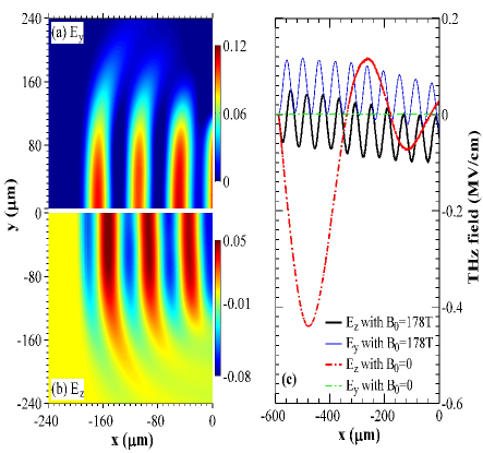
Figure 1: [(a) and (b)] Snapshots of the THz electric fields (MV/cm) at the time of 0.7 ps and (c) the field distributions on the axis ($y=0$) at 2 ps, where an external B field of 178T is imposed. The broken lines in (c) correspond to the case without the B field.

Figure 1 shows spatial distributions of the THz radiation propagating along the -x direction in the vacuum, which is generated with an external static B field of 178T imposed along the +x direction. As a comparison, the radiation generated without the B field is also displayed by the broken lines in Fig. 1(c), illustrating that the radiation has only the z-direction component and a near single-cycle waveform, as shown in previous experiments and simulations Cook ; Bartel ; Xie ; Kim ; THz_OE . With the B field, the radiation also has the y-direction component in addition to the z-direction one. The two components have the same frequency, higher than that in the case without the B field, and a constant phase displacement.

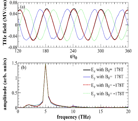
Figure 2: (a) Temporal waveforms of the THz electric fields on the axis and (b) the corresponding spectra, where an external B field of 178T is imposed. The components below 1 THz are filtered.

To further analyze the radiation properties, we take the temporal waveform observed in the left vacuum $5~{}\rm\mu m$ away from the vacuum-gas boundary, as illustrated in Fig. 2. The low-frequency part below 1 THz has been filtered and the high-frequency part is retained. One can see the radiation frequency at 5 THz, equal to the cyclotron frequency $\omega_{c}$. This frequency deviates from the central frequency around the plasma frequency $\omega_{p}=$ 1THz of the radiation without the B field.

Without the low-frequency or dc part, the two components $E_{y}$ and $E_{z}$ show nearly the same strength and a constant phase displacement of $\pi/2$, i.e., circular polarization. When we reverse the B field to -x direction, the phase displacement is changed to $-\pi/2$, i.e., the rotation of the CP radiation is also reversed, as observed in Fig 2. Note that, in real applications, the dc part of the radiation could be rapidly absorbed as soon as it touches a material rather than the vacuum. The effective radiation interacting with a sample should be a CP wave as shown in Fig. 2(a).

Now, we explain the radiation observed. The THz radiation process Kim ; THz_OE takes place as follows: first, a net current and plasma are formed via ionization, the current drives an electrostatic oscillating field in the plasma, and then this field is converted into electromagnetic radiation at the plasma boundaries. Without an external B field, electrons released from atoms have velocities only along the laser polarization, say the z direction, and therefore the generated radiation is also linearly polarized along the z direction. With the B field along the x direction, the electrons rotate in the y-z plane and then have velocities in both the y and z directions. Hence, the radiation has the components along both the y and z directions.

Frequency and waveform.$-$We set $E_{y}$ and $E_{z}$ as the radiation or oscillation electric fields formed in plasma. The nonrelativistic motion equation of an electron is $dv_{y}/dt=-eE_{y}/m_{e}-\omega_{c}v_{z}$ and $dv_{z}/dt=-eE_{z}/m_{e}+\omega_{c}v_{y}$, where both the external B field and the radiation fields much below relativistic strengthes are considered. One easily derives

$$\frac{d{\cal V}}{dt}=-\frac{e{\cal E}}{m_{e}}-i\omega_{c}{\cal V},$$ (1)

where ${\cal V}=v_{y}+iv_{z}$, ${\cal E}=E_{y}+iE_{z}$, and $i$ is the imaginary unit. According to the wave equation $(\nabla^{2}-\partial^{2}/c^{2}\partial t^{2})\mathbf{E}=-(4\pi en_{e}/c^{2})d\mathbf{v}/dt$ in plasma with a density $n_{e}$, one obtains

$$\left(\nabla^{2}-\frac{1}{c^{2}}\frac{\partial^{2}}{\partial t^{2}}\right){\cal E}=-\frac{4\pi en_{e}}{c^{2}}\frac{d{\cal V}}{dt}.$$ (2)

We first use Eq. (2) omitting the spatial differential term to look for the oscillation frequencies of the radiation source at a given position. Set ${\cal V}$ and ${\cal E}$ with a frequency $\omega$. According to Eqs. (1) and (2), one obtains:

$$\omega_{\pm}=\sqrt{\omega_{p}^{2}+\frac{\omega_{c}^{2}}{4}}\pm\frac{\omega_{c}}{2}.$$ (3)

Note that one can derive $\omega=\omega_{p}$ from Eqs. (1) and (2) in the same way for $B_{0}=0$. The three frequencies $\omega_{p}$ and $\omega_{\pm}$ correspond to the cutoff frequencies for wave propagation in unmagnetized and magnetized cold plasmas, respectively Bplasma_physics . The B field separates the oscillation frequency from $\omega_{p}$ into two frequencies: one above $\omega_{p}$ and the other below it. In particular, when $\omega_{c}\gg\omega_{p}$, $\omega_{+}$ approaches $\omega_{c}$, which provides a robust method to control the radiation frequency by the B-field strength. The simulation results in Fig. 2 and the red line in Fig. 3(b) are in good agreement with Eq. (3). The theoretical values are 5.19 THz and 0.19 THz, compared to 5 THz and 0 THz in the simulations with the numerical resolution of 0.5 THz.

Performing Fourier transform to Eqs. (1) and (2), one obtains the dispersion relation of the radiation wave along the -x direction, which has the refractive index $\eta=\sqrt{1-\omega_{p}^{2}/(\omega^{2}+\omega\omega_{c}})$. Under the condition of $\omega_{+}\simeq\omega_{c}\gg\omega_{p}$, $\eta\simeq 1$, and therefore, the $\omega_{+}$ component of the radiation generated even in deep plasma can propagate to the vacuum with little attenuation P.Gibbon . Hence, the radiation is many-cycle and narrow-band as shown in Figs. 1 and 2. This is different from the single-cycle and broadband radiation without the B field because of its central frequency at $\omega_{p}$ and $\eta=0$.

Polarization.$-$Since high-B fields are required by frequency-tunable radiation, we consider such B fields as

$$\omega_{L}\gg\omega_{c}\gg\omega_{p},$$ (4)

where $\omega_{L}$ is the laser fundamental frequency. With $\omega_{c}\gg\omega_{p}$, the B field dominates over the plasma oscillation, and thus, the velocity of an electron satisfies $v_{y,j}=v_{j}\cos(\omega_{c}t+\theta_{j})$ and $v_{z,j}=v_{j}\sin(\omega_{c}t+\theta_{j})$. With $\omega_{L}\gg\omega_{c}$ the initial phase $\theta_{j}$ can be considered as roughly the same for all electrons, since they are released only at the laser peak within a few cycles THz_PRE when 50fs laser duration is used here. Then the average electron velocity just after the passage of the pulses can be written by

$$\left\{{\begin{array}[]{l}{v_{y0}=v_{0}\cos(\omega_{c}t+\theta_{0}),}\\ {v_{z0}=v_{0}\sin(\omega_{c}t+\theta_{0}).}\end{array}}\right.$$ (7)

We replace the electric fields with the vector potentials $A_{y}$ and $A_{z}$ in Eqs. (1) and (2). From the two equations, one obtains $d{\cal V}/dt=(e/m_{e}c)d{\cal A}/dt-i\omega_{c}{\cal V}$ and $(\nabla^{2}-\partial^{2}/c^{2}\partial t^{2}){\cal A}=(4\pi en_{e}/c){\cal V}$, respectively, where ${\cal A}=A_{y}+iA_{z}$. Here we are interested in the higher-frequency component with $\omega_{+}\gg\omega_{p}$. This component with $\eta\simeq 1$ can propagate in the plasma as in a vacuum, which could be considered as a plane wave. Therefore, the corresponding electron velocity follows $-i\omega_{+}{\cal V}\simeq d{\cal V}/dt$ and $-i\omega_{c}{\cal V}\simeq(\omega_{c}/\omega_{+})d{\cal V}/dt$, with which the motion equation is rewritten by $(1-\omega_{c}/\omega_{+})({\cal V}-{\cal V}_{0})=(e/m_{e}c){\cal A}$. Inserting this equation of motion into the wave equation expressed by ${\cal A}$, one obtains

$$\left[\nabla^{2}-\frac{1}{c^{2}}\frac{\partial^{2}}{\partial t^{2}}-\frac{\omega_{p}^{2}}{c^{2}(1-\omega_{c}/\omega_{+})}\right]{\cal A}=\frac{4\pi en_{e}}{c}{\cal V}_{0},$$ (8)

where ${\cal V}_{0}$ is given by Eq. (7). Equation (8) describes radiation generation from a system forced by an temporally varying external source. It is difficult to solve analytically although a solution was given in THz_PoP under the condition of $B_{0}=0$ due to the source term independent of time. Obviously both the y and z components of the radiation have a strength linearly proportional to $v_{0}$ according to Eq. (7). The two components have a phase displacement fixed at $\pi/2$ which is determined by the one between $v_{y0}$ and $v_{z0}$. Therefore, the radiation at $\omega_{+}$ is CP. The rotation of ${\cal V}_{0}$ and the radiation will be reversed provided the B field sign is changed. These agree with the simulation results above.

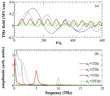
Figure 3: (a) Temporal waveforms of the THz electric fields $E_{y}$ on the axis and (b) the corresponding spectra, where different lines correspond to different $\omega_{c}$ ($\omega_{c}=$ 1THz corresponds to $B_{0}=$ 35.7T).

To further study the radiation features, we vary the B-field strength and gas density in the following simulations as shown in Figs. 3 and 4. Figure 3 illustrates that with an enhanced B field and $\omega_{c}=10$ THz, the radiation frequency, polarization, and waveform agree well with the analysis since the condition given in Eq. (4) is sufficiently met. With $\omega_{c}=2$ THz the simulation results roughly agree with the analysis. When $\omega_{c}=\omega_{p}=1$ THz, the radiation still has the $E_{y}$ component and its spectrum within 0.5-1.5 THz agrees with Eq. (3). Its waveform attenuates with time, approaching the one without the B field, because its frequency is close to $\omega_{p}$.

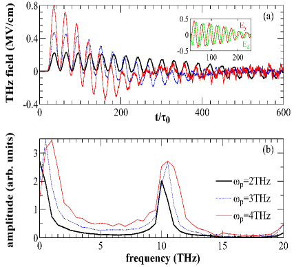
Figure 4: (a) Temporal waveforms of the THz electric fields $E_{y}$ on the axis and (b) the corresponding spectra, where different lines correspond to different $\omega_{p}$ or gas densities. The B field strength is fixed at 357T. The inset in (a) shows the radiation fields $E_{y}$ and $E_{z}$ with $\omega_{p}=$ 4 THz and the components below 2 THz are filtered.

In Fig. 4 we take different gas densities: $4.9\times 10^{16}~{}\rm cm^{-3}$, $1.1\times 10^{17}~{}\rm cm^{-3}$, and $1.96\times 10^{17}~{}\rm cm^{-3}$ with the corresponding $\omega_{p}=$ 2, 3 and 4 THz. The radiation frequencies agree well with Eq. (3). The radiation has a many-cycle waveform but the temporal attenuation of the waveform becomes more obvious with the growing density since the frequency $\omega_{+}$ is closer to $\omega_{p}$. The radiation is nearly CP even with $\omega_{p}=$ 4 THz, as observed in the inset in Fig. 4(a), provided the lower-frequency component is filtered. Note that as $\omega_{-}$ increases with the growing $\omega_{p}$, the field envelope tends to oscillate around the axis ($E_{y}=0$).

Table 1: Strength (MV/cm) of CP THz radiation of the $\omega_{+}$ component as a function of $\omega_{c}$ (the row) and $\omega_{p}$ (the column), where $\omega_{c}=$ 2THz corresponds to $B_{0}=$ 71T.

	2 THz	5 THz	10 THz	15 THz	20 THz	30 THz
1 THz	0.13	0.054	0.027	0.016	0.013	0.009
2 THz			0.12
3 THz			0.23
4 THz			0.41	0.27	0.20	0.12

We list the radiation strengths obtained in simulations as a function of $\omega_{c}$ and $\omega_{p}$ in Table I. It is shown that the radiation strength roughly follows:

$$E_{THz}^{\omega_{+}}\propto\frac{\omega_{p}^{2}}{\omega_{c}}.$$ (9)

According to Eq. (8), the strength scales linearly with the plasma density or the net current strength, i.e., $E_{THz}^{\omega_{+}}\propto\omega_{p}^{2}$. With a given plasma density, the current strength is nearly not changed with the B field. Multiplying the electron motion equation by the electron velocity $\mathbf{v}$, one obtains $dv^{2}/dt=-2e\mathbf{E}\cdot\mathbf{v}/m_{e}$, where $\mathbf{E}$ is the laser electric fields. When the B field satisfies Eq. (4) and tens of fs laser durations are considered here, the rotation of $\mathbf{v}$ from the laser polarization plane is slight during the laser interaction with the electron and therefore, the net gain of the electron energy (also the radiation energy) is nearly the same as the case without the B field. With a given radiation energy, the radiation strength will decrease linearly with its frequency $\omega_{+}\simeq\omega_{c}$, i.e., $E_{THz}^{\omega_{+}}\propto 1/\omega_{c}$.

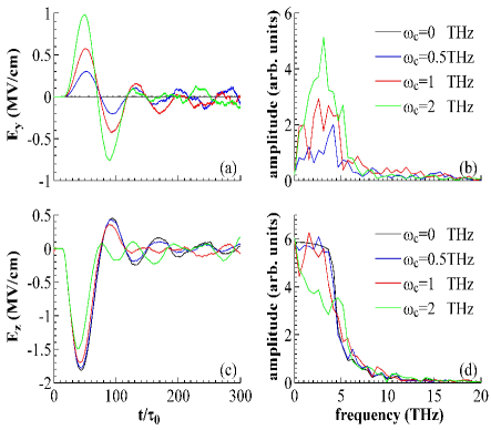
Figure 5: [(a) and (c) ]Temporal waveforms of the THz electric fields on the axis and [(b) and (d)] the corresponding spectra, where the gas density is taken as $1.96\times 10^{17}~{}\rm cm^{-3}$ ($\omega_{p}=$ 4THz) and different lines correspond to different $\omega_{c}$ ($\omega_{c}=$ 0.5THz corresponds to $B_{0}=$ 17.8T).

Next, we consider relatively low B fields with $\omega_{c}<\omega_{p}$ as shown in Fig. 5. EP radiation is also generated even with $B_{0}=$ 17.8T or $\omega_{c}=$ 0.5THz. The amplitude of $E_{y}$ grows with the B-field strength since more electron energy is transferred to the y direction by the B field. Both $E_{y}$ and $E_{z}$ have near single-cycle waveforms since their frequencies are close to $\omega_{p}$. The two-frequency spectrum disappears due to a low value of $\omega_{c}$. The relative phase is difficult to calculate since the radiation is broadband. We filter the low-frequency part below 1THz (such filter could be more meaningful for a spectrum with two frequencies separated) and the relative phase is changed from $0.8\pi$ to around $0.5\pi$ as $\omega_{c}$ grows from 0.5THz to 4THz.

The radiation with either a high or low B field is generated due to the gyrational motion of plasma electrons under the B field. This field slightly affects the gas ionization responsible for the current formation. Hence the magnetic approach can be extended to other laser-plasma-based THz emission schemes, which has been verified by our simulations with an asymmetric-laser scheme THz_PoP . Besides, we have performed a 3D PIC simulation and observed the same result as a 2D simulation with the same parameters as in Fig. 1 but with a plane laser driver. The result also approaches that with $r_{0}=150\rm\mu m$ in Fig. 1(c), indicating that our study is valid with a larger spot radius $r_{0}$.

In summary, we have demonstrated a unique EP or CP, narrow-band THz source if a static B field is applied. With a high B field at a 100T scale, the radiation shows two frequencies: the lower is nearly dc and the higher (central frequency) almost at $\omega_{c}$. Therefore, the central frequency can be adjusted linearly by the B-field strength. The radiation rotation can also be controlled by the B-field sign. With the B field decreased to the 10T scale, EP radiation is still generated but becomes broadband and single cycle. To fully apply this scheme under the high-B-field condition in Eq. (4) to the whole THz band, the B-field strength should be tunable within 3.57T to 357T (corresponding to 0.1THz to 10THz). Besides the B-fields generated in traditional ways Labs_highB ; B600T ; B310T , one may employ novel nanosecond-laser-driven superstrong B-fields Fujioka ; Lasest_Bfield with the strength continuously tunable by the laser energy and with a duration of nanoseconds (far longer than THz radiation cycle). With this source, one can realize the magnetically controlled two-color scheme in an all-optical way, where the B-field generation is easily synchronized with the two-color laser driver.

- (1) D. Grischkowsky, S. Keiding, M. Exter, and C. Fattinger, J. Opt. Soc. Am. B 7, 2006 2015 (1990).
- (2) J. C. Cao, Phys. Rev. Lett. 91, 237401 (2003).
- (3) M. Jewariya, M. Nagai, and K. Tanaka, Phys. Rev. Lett. 105, 203003 (2010).
- (4) T. Kampfrath, K. Tanaka, and K. Nelson, Nat. Photonics 7, 680 (2013).
- (5) B. Alexandrov, M. Phipps, L. Alexandrov, L. Booshehri, A. Erat, J. Zabolotny, C. Mielke, H.-T. Chen, G. Rodriguez, K. Rasmussen et al., Sci. Rep. 3, 1184 (2013).
- (6) R. Woodward, V. Wallace, R. Pye, B. Cole, D. Arnone, E. Linfield, and M. Pepper, J. Invest. Dermatol. 120, 72 (2003).
- (7) D. J. Cook and R. M. Hochstrasser, Opt. Lett. 25, 1210 (2000).
- (8) M. Kress, T. Loffler, S. Eden, M. Thomson, and H. G. Roskos, Opt. Lett. 29, 1120 (2004).
- (9) T. Bartel, P. Gaal, K. Reimann, M. Woerner, and T. Elsaesser, Opt. Lett. 30, 2805 (2005).
- (10) X. Xie, J. Dai, and X.-C. Zhang, Phys. Rev. Lett. 96, 075005 (2006).
- (11) K. Y. Kim, J. H. Glownia, A. J. Taylor and G. Rodriguez, Opt. Express 15, 4577 (2007).
- (12) W.-M. Wang, Z.-M. Sheng, H.-C. Wu, M. Chen, C. Li, J. Zhang, and K. Mima, Opt. Express 16, 16999 (2008).
- (13) X.-Y. Peng, C. Li, M. Chen, T. Toncian, R. Jung, O. Willi, Y.-T. Li, W.-M. Wang, S.-J. Wang, F. Liu et al., Appl. Phys. Lett. 94, 101502 (2009).
- (14) T.-J. Wang, Y. Chen, C. Marceau, F. Theberge, M. Chateauneuf, J. Dubois, and S. L. Chin, Appl. Phys. Lett. 95, 131108 (2009).
- (15) Y. Chen, T.-J. Wang, C. Marceau, F. Theberge, M. Chateauneuf, J. Dubois, O. Kosareva and S. L. Chin, Appl. Phys. Lett. 95, 101101 (2009).
- (16) W.-M. Wang, Z.-M. Sheng, Y.-T. Li, L. M. Chen, Q.-L. Dong, X. Lu, J.-L. Ma, and J. Zhang, Chin. Opt. Lett. 9, 110002 (2011) (Invited Paper).
- (17) Y. S. You, T. I. Oh, and K. Y. Kim, Phys. Rev. Lett. 109, 183902 (2012).
- (18) W.-M. Wang, Y.-T. Li, Z.-M. Sheng, X. Lu, and J. Zhang, Phys. Rev. E 87, 033108 (2013).
- (19) W.-M. Wang, P. Gibbon, Z.-M. Sheng, and Y.-T. Li, Phys. Rev. A 90, 023808 (2014).
- (20) Y. T. Li, C. Li, M. L. Zhou, W. M. Wang, F. Du, W. J. Ding, X. X. Lin, F. Liu, Z. M. Sheng, X. Y. Peng et al., Appl. Phys. Lett. 100, 254101 (2012); G.Q. Liao et al., Phys. Rev. Lett. 114, 255001 (2015).
- (21) A. Gopal, S. Herzer, A. Schmidt, P. Singh, A. Reinhard, W. Ziegler, D. Brommel, A. Karmakar, P. Gibbon, U. Dillner et al., Phys. Rev. Lett. 111, 074802 (2013).
- (22) M. Clerici, M. Peccianti, B. E. Schmidt, L. Caspani, M. Shalaby, M. Giguere, A. Lotti, A. Couairon, F. Legare, T. Ozaki et al., Phys. Rev. Lett. 110, 253901 (2013).
- (23) T. I. Oh, Y. J. Yoo, Y. S. You, and K. Y. Kim, Appl. Phys. Lett. 105, 041103 (2014).
- (24) Y. S. You, T. I. Oh, and K.-Y. Kim, Opt. Lett. 38, 1034 (2013).
- (25) S. Spielman, B. Parks, J. Orenstein, D. T. Nemeth, F. Ludwig, J. Clarke, P. Merchant, and D. J. Lew, Phys. Rev. Lett. 73, 1537(1994).
- (26) J. Xu, J. Galan, G. Ramian, P. Savvidis, A. Scopatz, R. R. Birge, S. J. Allen, and K. Plaxco, Proc. SPIE 5268, 19 (2004).
- (27) X. Wang, Y. Cui, W. Sun, J. Ye, and Y. Zhang, J. Opt. Soc. Am. A 27, 2387 (2010).
- (28) H. C. Wu, J. Meyer-ter-Vehn, and Z. M. Sheng, New J. Phys. 10, 043001 (2008).
- (29) J. Dai, N. Karpowicz, and X.-C. Zhang, Phys. Rev. Lett. 103, 023001 (2009).
- (30) H. Wen and A. M. Lindenberg, Phys. Rev. Lett. 103, 023902 (2009).
- (31) http://lbtuam.es/?page_id=212
- (32) Y. H. Matsuda, F. Herlach, S. Ikeda and N. Miura, Rev. Sci. Instrum. 73, 4288 (2002).
- (33) O. Portugall, N. Puhlmann, H. U. Muller, M. Barczewski, I. Stolpe and M. von Ortenberg, J. Phys. D. Appl. Phys. 32, 2354 (1999).
- (34) S. Fujioka, Z. Zhang, K. Ishihara, K. Shigemori, Y. Hironaka, T. Johzaki, A. Sunahare, N. Yamamoto, H. Nakashima, T. Watanabe et al., Sci. Rep. 3, 1170 (2013).
- (35) W.-M. Wang, P. Gibbon, Z.-M. Sheng, and Y.-T. Li, Phys. Rev. Lett. 114, 015001 (2015).
- (36) P. Y. Chang, G. Fiksel, M. Hohenberger, J. P. Knauer, R. Betti, F. J. Marshall, D. D. Meyerhofer, F. H. Seguin, and R. D. Petrasso, Phys. Rev. Lett. 107, 035006 (2011).
- (37) W.-M. Wang, P. Gibbon, Z.-M. Sheng, and Y.-T. Li, Phys. Rev. E 91, 013101 (2015).
- (38) T. J. M. Boyd and J. J. Sanderson, The Physics of Plasmas (Cambridge University Press, 2003, Chapter 6).
- (39) P. Gibbon, Short Pulse Laser Interactions with Matter (Imperial College Press, 2000).
- (40) W.-M. Wang, S. Kawata, Z.-M. Sheng, Y.-T. Li, and J. Zhang, Phys. Plasmas 18, 073108 (2011).
- (41) J. J. Santos et al., Laser-driven platform for generation and characterization of strong quasi-static magnetic fields (http://arxiv.org/abs/1503.00247).