Boltzmann-conserving classical dynamics in quantum time-correlation functions: ‘Matsubara dynamics’

Abstract

We show that a single change in the derivation of the linearized semiclassical-initial value representation (LSC-IVR or ‘classical Wigner approximation’) results in a classical dynamics which conserves the quantum Boltzmann distribution. We rederive the (standard) LSC-IVR approach by writing the (exact) quantum time-correlation function in terms of the normal modes of a free ring-polymer (i.e. a discrete imaginary-time Feynman path), taking the limit that the number of polymer beads $N\rightarrow\infty$, such that the lowest normal-mode frequencies take their ‘Matsubara’ values. The change we propose is to truncate the quantum Liouvillian, not explicitly in powers of $\hbar^{2}$ at $\hbar^{0}$ (which gives back the standard LSC-IVR approximation), but in the normal-mode derivatives corresponding to the lowest Matsubara frequencies. The resulting ‘Matsubara’ dynamics is inherently classical (since all terms ${\cal O}(\hbar^{2})$ disappear from the Matsubara Liouvillian in the limit $N\rightarrow\infty$), and conserves the quantum Boltzmann distribution because the Matsubara Hamiltonian is symmetric with respect to imaginary-time translation. Numerical tests show that the Matsubara approximation to the quantum time-correlation function converges with respect to the number of modes, and gives better agreement than LSC-IVR with the exact quantum result. Matsubara dynamics is too computationally expensive to be applied to complex systems, but its further approximation may lead to practical methods. Copyright (2015) American Institute of Physics. This article may be downloaded for personal use only. Any other use requires prior permission of the author and the American Institute of Physics. The following article appeared in the Journal of Chemical Physics, 142, 134103 (2015) and may be found at http://dx.doi.org/10.1063/1.4916311

I Introduction

Dynamical properties at thermal equilibrium are of central importance to chemical physics.green ; daan Sometimes these properties can be simulated adequately by entirely classical means. But there are plenty of cases, e.g. the spectrum of liquid water,rpmd_water ; lsc-ivr_water ; marx_water hydrogen-diffusion on metals,aedes ; yury and proton/hydride-transfer reactions,hammes1 ; tmiller1 ; mano_borg ; makri1 ; shi ; rommel for which one needs to evaluate time-correlation functions of the form

$${1\over Z}\overline{C}_{AB}(t)={1\over Z}{\rm Tr}\left[e^{-\beta\hat{H}}\hat{A}e^{i\hat{H}t/\hbar}\hat{B}e^{-i\hat{H}t/\hbar}\right]$$ (1)

(where $Z$ is the partition function,def $\beta\equiv 1/k_{\rm B}T$, Tr indicates a complete sum over states, and the other notation is defined in Sec. II). Such time-correlation functions are already approximate, since they employ the quantum Boltzmann distribution $e^{-\beta\hat{H}}/Z$ in place of the exact quantum-exchange statistics; but this approximation is usually adequate (since the thermal wavelength is typically much smaller than the separations between identical particles). What is less well understood is the extent to which such functions can be further approximated by replacing the exact quantum dynamics by classical dynamics (whilst retaining the quantum Boltzmann statistics).

The standard way to make this approximation is to use the linearized semiclassical-initial value representation (LSC-IVR, sometimes called the ‘classical Wigner’ approximation),lsc-ivr_water ; miller_rev ; wang_miller ; miller_molphys ; liumill ; poulsen ; coker1 ; coker2 ; shi_geva ; hillery ; heller ; Shig2 ; Liurev ; borgis in which the quantum Liouvillian is expanded as a power series in $\hbar^{2}$, then truncated at $\hbar^{0}$. Millermiller_rev ; miller_molphys and later Shi and Gevashi_geva showed that this approximation is equivalent to linearizing the displacement between forward and backward Feynman paths in the exact quantum time-propagation, which removes the coherences, thus making the dynamics classical. The LSC-IVR retains the Boltzmann quantum statistics inside a Wigner transform,hillery is exact in the zero-time, harmonic and high-temperature limits, and has been developed into a practical method by several authors.liumill ; Shig2 ; poulsen ; Liurev ; borgis However, it has a serious drawback: the classical dynamics does not in general preserve the quantum Boltzmann distribution, and thus the quality of the statistics deteriorates over time.

A number of methods have been developed to get round this problem, all of which appear to some extent to be ad hoc. Some of these methods are obtained by replacing the plain Newtonian dynamics in the LSC-IVR by an effective (classical) dynamics which preserves the Boltzmann distribution.liu1 ; liu2 ; poul1 Others, such as the popular centroid molecular dynamics (CMD)jang ; rossky and ring-polymer molecular dynamics (RPMD),rpmd_water ; yury ; tmiller1 ; mano_borg ; craig1 ; craig2 ; craig3 ; markman ; rpmd_rev ; tmiller3 ; tmiller4 ; kinetic ; nandini1 ; yury2 ; huo1 ; huoaoiz ; rossky2 ; trpmd ; jeremy ; tim1 ; tim2 ; tim3 ; tim_thesis ; jeremy_new ; conan2 are more heuristic (and still not fully understood) but have the advantage that they can be implemented directly in classical molecular dynamics codes. An intriguing property of CMD and RPMD is that, for some model systems (e.g. the one-dimensional quartic oscillatorcraig1 ; rossky ), these methods give better agreement than LSC-IVR with the exact quantum result, even though, like LSC-IVR, they completely neglect real-time quantum coherence.

This last point suggests that the failure of LSC-IVR to preserve the quantum Boltzmann distribution may arise, not from its neglect of quantum coherence, but from its inclusion of ‘rogue’ components in the classical dynamics. The present paper develops a theory that supports this speculation. We isolate a core, Boltzmann-conserving, classical dynamics, which we call ‘Matsubara dynamics’ (for reasons to be made clear). Matsubara dynamics is far too expensive to be used as a practical method, but is likely to prove useful in understanding methods such as CMD and RPMD, and perhaps in developing new approximate methods.

The paper is structured as follows. Section II gives key background material including the well known ‘Moyal series’ derivation of the LSC-IVR. Section III re-expresses the standard results of Sec. II in terms of ‘ring-polymer’ coordinates, involving points along the imaginary-time path-integrals that describe the quantum Boltzmann statistics. Section IV gives the new results, showing that smooth Fourier-transformed combinations of the ring-polymer coordinates lead to an inherently classical dynamics which is quantum-Boltzmann-conserving. Section V reports numerical tests on one-dimensional models. Section VI concludes the article.

II Background theory

We start by defining the terms and notation to be used in classical and quantum Boltzmann time-correlation functions (IIA and IIB), and by writing out the standard Moyal-series derivation of the LSC-IVR (IIC).

II.1 Classical correlation functions

Without loss of generality, we can consider an $F$-dimensional Cartesian system with position coordinates ${\bf q}\equiv q_{1},\ldots,q_{F}$, momenta ${\bf p}$, mass $m$ and Hamiltonian

$$H({\bf p},{\bf q})=\frac{{\bf p}^{2}}{2m}+V({\bf q})$$ (2)

The thermal time-correlation function between observables $A({\bf p},{\bf q})$, $B({\bf p},{\bf q})$ is then

$$c_{AB}(t)= \frac{1}{(2\pi\hbar)^{N}}\int d{\bf p}\int d{\bf q}\ e^{-\beta H({\bf p},{\bf q})}$$

$$\times A({\bf p},{\bf q})B({\bf p}_{t},{\bf q}_{t})$$ (3)

where $\int d{\bf p}\equiv\int_{-\infty}^{\infty}dp_{1}\ldots\int_{-\infty}^{\infty}dp_{F}$ (and similarly for ${\bf q}$), and ${\bf p}_{t}\equiv{\bf p}_{t}({\bf p},{\bf q},t)$ and ${\bf q}_{t}\equiv{\bf q}_{t}({\bf p},{\bf q},t)$ are the momenta and positions after the classical dynamics has evolved for a time $t$.

Alternatively, we can express $B({\bf p}_{t},{\bf q}_{t})$ as a function of the initial phase-space coordinates $({\bf p},{\bf q})$:

$$B({\bf p}_{t},{\bf q}_{t})\equiv B[{\bf p}_{t}({\bf p},{\bf q},t),{\bf q}_{t}({\bf p},{\bf q},t)]\equiv B({\bf p},{\bf q},t)$$ (4)

such that

$$c_{AB}(t)= \frac{1}{(2\pi\hbar)^{N}}\int d{\bf p}\int d{\bf q}\ e^{-\beta H({\bf p},{\bf q})}$$

$$\times A({\bf p},{\bf q})B({\bf p},{\bf q},t)$$

$$= \frac{1}{(2\pi\hbar)^{N}}\int d{\bf p}\int d{\bf q}\ e^{-\beta H({\bf p},{\bf q})}$$

$$\times A({\bf p},{\bf q})e^{{\cal L}_{F}t}B({\bf p},{\bf q},0)$$ (5)

where the (classical) Liouvillian ${\cal L}_{F}$ iszwanzig

$${\cal L}_{F}={1\over m}{\bf p}\cdot{\bf\nabla_{q}}-V({\bf q})\overleftarrow{\nabla}_{\bf q}\cdot\overrightarrow{\nabla}_{\bf p}$$ (6)

with

$$\nabla_{\bf q}=\left(\!\begin{array}[]{c}\frac{\partial}{\partial q_{1}}\\ \vdots\\ \frac{\partial}{\partial q_{F}}\end{array}\!\right)$$ (10)

and the arrows indicate the direction in which the derivative operator is applied (and the backward arrow indicates that the derivative is taken only of $V({\bf q})$—not of any terms that may precede $V({\bf q})$ in any integral). Equation (5) is less practical than Eq. (3) (which propagates individual trajectories rather than the distribution function $B({\bf p},{\bf q},t)$) but is better for comparison with the exact quantum expression.

An essential property of the dynamics is that it preserves the (classical) Boltzmann distribution, which follows because $H({\bf p},{\bf q})$ is a constant of the motion. As a result, we can rearrange Eq. (5) as

$$c_{AB}(t)= \frac{1}{(2\pi\hbar)^{N}}\int d{\bf p}\int d{\bf q}\ e^{-\beta H({\bf p},{\bf q})}$$

$$\times\left[e^{-{\cal L}_{F}t}A({\bf p},{\bf q})\right]B({\bf p},{\bf q},0)$$ (11)

showing that $c_{AB}(t)$ satisfies

$$c_{AB}(t)=c_{BA}(-t)$$ (12)

which is the detailed balance condition.

II.2 Quantum correlation functions

For clarity of presentation, we will derive the results in Secs. III and IV for a one-dimensional quantum system with Hamiltonian $\hat{H}=\hat{T}+\hat{V}$, kinetic energy operator $\hat{T}=\hat{p}^{2}/2m$, potential energy operator $\hat{V}=V(\hat{q})$, position and momentum operators ${\hat{q},\hat{p}}$, and mass $m$. However, the results we derive in Secs. III and IV are applicable immediately to systems with any number of dimensions (see Sec. IV.D).

The simplest form of quantum-Boltzmann time-correlation function is that given in Eq. (1), but ${\overline{C}}_{AB}(t)$ is difficult to relate to the classical time-correlation function $c_{AB}(t)$, because it does not satisfy Eq. (12) and is not in general real. We therefore use the Kubo-transformed time-correlation functioncraig1

$$C_{AB}(t)={\rm Tr}\left[K_{\beta}({\hat{A}})\,e^{i\hat{H}t/\hbar}\hat{B}e^{-i\hat{H}t/\hbar}\right]$$ (13)

with

$$K_{\beta}({\hat{A}})=\frac{1}{\beta}\int_{0}^{\beta}d\lambda\ e^{-\lambda\hat{H}}\hat{A}e^{-(\beta-\lambda)\hat{H}}$$ (14)

This function gives an equivalent description of the dynamics to ${\overline{C}}_{AB}(t)$, to which it is related by a simple Fourier-transform formula.craig1

It is easy to show (by noting that $e^{-\lambda\hat{H}}$ and $e^{-i\hat{H}t/\hbar}$ commute in Eq. (13)) that ${C}_{AB}(t)$ satisfies the detailed balance relation

$$C_{AB}(t)=C_{BA}(-t)$$ (15)

This relation also ensures that ${C}_{AB}(t)$ is real (since reversing the order of operators in the trace gives $C_{AB}(t)=C_{BA}^{*}(-t)$).

The $t=0$ limit of $C_{AB}(t)$ can be expressedcraig1 in terms of a classical Boltzmann distribution over an extended phase space of ‘ring-polymers’.chandler_wolynes ; parrinello ; ceperley ; charu When ${\hat{A}}$ and ${\hat{B}}$ are functions ${A}(\hat{q})$ and ${B}(\hat{q})$ of the position operator $\hat{q}$, the ring-polymer expression is

$$C_{AB}(0)= \lim_{N\to\infty}{1\over(2\pi\hbar)^{N}}\int\!d{\bf p}\int\!d{\bf q}\$$

$$\times A({\bf q})B({\bf q})e^{-\beta_{N}R_{N}({\bf p},{\bf q})}$$ (16)

where $\beta_{N}=\beta/N$, $\int\!d{\bf p}\equiv\int_{-\infty}^{\infty}d{p_{1}}\dots\int_{-\infty}^{\infty}d{p_{N}}$ and similarly for $\int\!d{\bf q}$, and

$$A({\bf q})= \frac{1}{N}\sum_{i=1}^{N}A({q}_{i}),\qquad B({\bf q})=\frac{1}{N}\sum_{i=1}^{N}B({q}_{i})$$ (17)

$$R_{N}({\bf p},{\bf q})= T_{N}({\bf p},{\bf q})+U_{N}({\bf q})$$ (18)

$$T_{N}({\bf p},{\bf q})= {{\bf p}^{2}\over 2m}+{m\over 2(\beta_{N}\hbar)^{2}}\sum_{i=1}^{N}(q_{i+1}-q_{i})^{2}$$ (19)

$$U_{N}({\bf q})= \sum_{i=1}^{N}V(q_{i})$$ (20)

Similar expressions can be obtained when ${\hat{A}}$ and ${\hat{B}}$ depend on the momentum operator (by inserting position-momentum Fourier-transforms). To avoid confusion, we emphasise that Eq. (16) is exact at $t=0$, and that we do not assume that the ring-polymer Hamiltonian $R_{N}({\bf p},{\bf q})$ generates the dynamics at $t>0$.

II.3 The LSC-IVR approximation

II.3.1 The Wigner-Moyal series

To derive the LSC-IVR approximation to $C_{AB}(t)$, we follow ref. hillery, , expanding the exact quantum Liouvillian in powers of $\hbar^{2}$. We start by rewriting Eq. (13) as

$$C_{AB}(t)= \int_{-\infty}^{\infty}dq\int_{-\infty}^{\infty}d\Delta$$

$$\times\langle q-\Delta/2|K_{\beta}({\hat{A}})|q+\Delta/2\rangle$$

$$\times\langle q+\Delta/2|e^{i\hat{H}t/\hbar}\hat{B}e^{-i\hat{H}t/\hbar}|q-\Delta/2\rangle$$ (21)

then insert the momentum identity

$$\delta(\Delta-\Delta^{\prime})={1\over 2\pi\hbar}\int_{-\infty}^{\infty}dp\ e^{ip(\Delta-\Delta^{\prime})/\hbar}$$ (22)

to obtain

$$C_{AB}(t)= \frac{1}{2\pi\hbar}\int_{-\infty}^{\infty}dq\int_{-\infty}^{\infty}dp$$

$$\times[K_{\beta}({\hat{A}})]_{\rm W}(p,q)\,[\hat{B}(t)]_{\rm W}(p,q)$$ (23)

where the Wigner transforms of $\hat{A}$ and $\hat{B}$ are given by

$$[K_{\beta}({\hat{A}})]_{\rm W}(p,q)= \int_{-\infty}^{\infty}d\Delta e^{ip\Delta/\hbar}$$

$$\times\langle q-\Delta/2|K_{\beta}({\hat{A}})|q+\Delta/2\rangle$$ (24)

and

$$[\hat{B}(t)]_{\rm W}(p,q)= \int_{-\infty}^{\infty}d\Delta\ e^{ip\Delta/\hbar}$$

$$\times\langle q-\Delta/2|e^{i\hat{H}t/\hbar}\hat{B}e^{-i\hat{H}t/\hbar}|q+\Delta/2\rangle.$$ (25)

(and note that we will often suppress the $(p,q)$ dependence of $[K_{\beta}({\hat{A}})]_{\rm W}$ and $[\hat{B}(t)]_{\rm W}$).

We then differentiate Eq. (23) with respect to $t$,

$${dC_{AB}(t)\over dt}= \frac{1}{2\pi\hbar}\int_{-\infty}^{\infty}dq\int_{-\infty}^{\infty}dp$$

$$\times[K_{\beta}({\hat{A}})]_{\rm W}\left[\frac{i}{\hbar}[\hat{H},\hat{B}(t)]\right]_{\rm W}$$ (26)

and expand the potential-energy operator in the commutator in powers of $\Delta$ to obtain

$$\left[\frac{i}{\hbar}[\hat{H},\hat{B}(t)]\right]_{\rm W}= \int_{-\infty}^{\infty}d\Delta\ e^{ip\Delta/\hbar}$$

$$\times{\hat{\ell}}\langle q-\Delta/2|\hat{B}(t)|q+\Delta/2\rangle$$ (27)

with

$${\hat{\ell}}=\frac{i\hbar}{m}\frac{\partial}{\partial q}\frac{\partial}{\partial\Delta}-{2i\over\hbar}\sum_{\lambda=1,{\rm odd}}^{\infty}{1\over\lambda!}{\partial^{\lambda}V(q)\over\partial q^{\lambda}}\left({\Delta\over 2}\right)^{\lambda}$$ (28)

Noting that each power of $\Delta$ can be generated by an application of ${-i\hbar\partial/\partial p}$, we then obtain

$$\frac{dC_{AB}(t)}{dt}= \frac{1}{2\pi\hbar}\int_{-\infty}^{\infty}\!dq\int_{-\infty}^{\infty}\!dp$$

$$\times[K_{\beta}({\hat{A}})]_{\rm W}\,{\hat{L}}[\hat{B}(t)]_{\rm W}$$ (29)

with

$$\hat{L}= \frac{p}{m}\frac{\partial}{\partial q}-\sum_{\lambda=1,{\rm odd}}^{\infty}{1\over\lambda!}\left({i\hbar\over 2}\right)^{\lambda-1}{\partial^{\lambda}V(q)\over\partial q^{\lambda}}{\partial^{\lambda}\over\partial p^{\lambda}}$$ (30)

This is the Moyal expansion of the quantum Liouvillian in powers of $\hbar^{2}$. If all terms are included in the series, then the application of $\hat{L}$ generates the exact quantum dynamics (as is easily proved by working backwards through the derivation just given). A compact representation of $\hat{L}$, which will be useful later on is,

$$\hat{L}= \frac{p}{m}\frac{\partial}{\partial q}-V(q)\frac{2}{\hbar}\sin\!\left(\frac{\overleftarrow{\partial}}{\partial q}\frac{\hbar}{2}\frac{\overrightarrow{\partial}}{\partial p}\right).$$ (31)

where the arrows are defined in the same way as in Eq. (6)

II.3.2 Approximating the dynamics

To obtain the LSC-IVR one notes that Eq. (30) can be written

$${\hat{L}}= \mathcal{L}+\mathcal{O}(\hbar^{2})$$ (32)

where $\mathcal{L}$ is the classical Liouvillian

$$\mathcal{L}=\frac{p}{m}\frac{\partial}{\partial q}-\frac{\partial V}{\partial q}\frac{\partial}{\partial p}$$ (33)

and then truncates ${\hat{L}}$ at $\hbar^{0}$. The LSC-IVR thus amounts to replacing the quantum dynamics by classical dynamics, such that $C_{AB}(t)$ is approximated by

$$C_{AB}^{\rm W}(t)= \int_{-\infty}^{\infty}\!dq\int_{-\infty}^{\infty}\!dp$$

$$\times[K_{\beta}({\hat{A}})]_{\rm W}(p,q)\,e^{\mathcal{L}t}[\hat{B}(0)]_{\rm W}({p},{q})$$ (34)

or equivalently

$$C_{AB}^{\rm W}(t)= \int_{-\infty}^{\infty}\!dq\int_{-\infty}^{\infty}\!dp$$

$$\times[K_{\beta}({\hat{A}})]_{\rm W}(p,q)\,[\hat{B}(0)]_{\rm W}({p}_{t},{q}_{t})$$ (35)

where $(p_{t},q_{t})$ are the (classical) position and momentum at time $t$ of a trajectory initiated at $(p,q)$ at $t=0$.

Physical insight into the LSC-IVR is obtained by going back to Eq. (28), and noting that truncating $\hat{L}$ at $\hbar^{0}$ is equivalent to truncating ${\hat{l}}$ at $\Delta$. Since $\Delta$ is the difference between the origin of a forward path that terminates at $z$ (at time $t$) and the terminus of a backward path that originates at $z$, it follows that truncating at $\Delta$ is equivalent to linearizing the difference between the forward and backward Feynman paths at each time-step. Hence the neglect of terms ${\cal O}(\hbar^{2})$ is valid if the forward and backward paths are very close together, in which case there are no coherence effects, and the dynamics becomes classical. The LSC-IVR is thus exact at $t=0$ (where the paths become infinitessimally short), in the harmonic limit (where the are no terms ${\cal O}(\hbar^{2})$ in $\hat{L}$), and in the high temperature limit (where fluctuations in $\Delta$ efficiently dephase).summar

Despite these positive features, LSC-IVR suffers from the major drawback of not preserving the quantum Boltzmann distribution (except in one of the special limits just mentioned), since in general

$$\mathcal{L}[e^{-\beta\hat{H}}]_{\rm W}\neq 0$$ (36)

As a result,

$$C_{AB}^{\rm W}(t) \neq C_{BA}^{\rm W}(-t)$$ (37)

i.e. the LSC-IVR does not satisfy detailed balance. In Secs. III-V we will investigate why this is so.

III Ring-polymer coordinates

We now recast the standard expressions of Sec. II in terms of ring-polymer coordinates. No new approximations are obtained, but the ring-polymer versions of these expressions are needed for use in Sec. IV, where they will be used to derive the quantum-Boltzmann-conserving ‘Matsubara’ dynamics.

III.1 Ring-polymer representation of Kubo-transformed time-correlation functions

III.1.1 Exact quantum time-correlation function

Following ref. tim1, (see also refs. shi_geva, and nandini1, ), we define the ring-polymer quantum time-correlation function to be

$$C_{AB}^{[N]}(t)= \int d{\bf q}\int d{\bf\Delta}\int d{\bf z}\ A({\bf q})B({\bf z})$$

$$\times\prod_{l=1}^{N}\langle q_{l-1}-\Delta_{l-1}/2|e^{-\beta_{N}\hat{H}}|q_{l}+\Delta_{l}/2\rangle$$

$$\qquad\times\langle q_{l}+\Delta_{l}/2|e^{-i\hat{H}t/\hbar}|z_{l}\rangle$$

$$\qquad\times\langle z_{l}|e^{i\hat{H}t/\hbar}|q_{l}-\Delta_{l}/2\rangle$$ (38)

where the functions $A({\bf q})$ and $B({\bf z})$ (with ${\bf z}$ in place of ${\bf q}$) are defined in Eq. (17) (and we have assumed that $\hat{A}$ and $\hat{B}$ are functions of position operators to simplify the algebra—see Sec. IVD). It is easy to show (by noting that $N\!-\!1$ of all the forward-backward propagators are identities, and that the sums in $A({\bf q})$ and $B({\bf z})$ become integrals in the limit $N\to\infty$) that

$$C_{AB}(t)=\lim_{N\rightarrow\infty}C_{AB}^{[N]}(t)$$ (39)

In other words, Eq. (38) in the limit $N\to\infty$ is just an alternative way of writing out the standard Kubo-transformed time-correlation function $C_{AB}(t)$. The advantage of Eq. (38) is that it emphasises the symmetry of the entire path-integral expression with respect to cyclic permutations of the coordinates $q_{l}\to q_{l+1}$ (see Fig. 1); this symmetry is otherwise hidden in the conventional expression for $C_{AB}(t)$ [Eq. (13)].

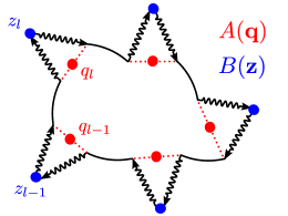
Figure 1: Schematic diagram showing the structure of the (exact) Kubo-transformed quantum time-correlation function when represented in ring-polymer coordinates as in Eq. (38). The red and blue dots represent the coordinates $q_{l}$ and $z_{l}$; solid lines represent stretches of imaginary time of length $\beta_{N}\hbar$; arrows represent forward-backward propagations in real time.

III.1.2 Ring-polymer representation of the LSC-IVR

It is straightforward to derive the LSC-IVR approximation from Eq. (38) by generalizing the steps in Sec. IIC. We insert an identity

$$\delta(\Delta_{l}-\Delta_{l}^{\prime})={1\over 2\pi\hbar}\int_{-\infty}^{\infty}dp_{l}\ e^{ip_{l}(\Delta_{l}-\Delta_{l}^{\prime})/\hbar}$$ (40)

for each value $l=1,\dots,N$, to obtain

$$C_{AB}^{[N]}(t)= {1\over(2\pi\hbar)^{N}}\int d{\bf q}\int d{\bf p}\left[e^{-\beta{\hat{H}}}{\hat{A}}\right]_{\overline{N}}({\bf p},{\bf q})\,\left[{\hat{B}}(t)\right]_{N}({\bf p},{\bf q})$$ (41)

where

$$\left[e^{-\beta{\hat{H}}}{\hat{A}}\right]_{\overline{N}}({\bf p},{\bf q})= \int d{\bf\Delta}\ A({\bf q})\prod_{l=1}^{N}\langle q_{l-1}-\Delta_{l-1}/2|e^{-\beta_{N}\hat{H}}|q_{l}+\Delta_{l}/2\rangle e^{ip_{l}\Delta_{l}/\hbar}$$ (42)

and

$$\left[{\hat{B}}(t)\right]_{N}({\bf p},{\bf q})= \int d{\bf\Delta}\int d{\bf z}\ B({\bf z})\prod_{l=1}^{N}\langle q_{l}-\Delta_{l}/2|e^{-i\hat{H}t/\hbar}|z_{l}\rangle\langle z_{l}|e^{i\hat{H}t/\hbar}|q_{l}+\Delta_{l}/2\rangle e^{ip_{l}\Delta_{l}/\hbar}$$ (43)

are generalized Wigner transforms (and we will often suppress the dependence on $({\bf p},{\bf q})$ in what follows). Note that $[\cdot]_{N}$ and $[\cdot]_{\overline{N}}$ have different forms: $[\cdot]_{N}$ is a sum of products of one-dimensional Wigner transforms, whereas $[\cdot]_{\overline{N}}$ is more complicated, with each product coupling variables in $l$ and $l+1$.alter Note that since we have specified that ${\hat{B}}$ is a function of just the position operator (in order to simplify the algebra—see Sec. IVD), it follows that

$$\left[{\hat{B}}(0)\right]_{N}({\bf p},{\bf q})=B({\bf q})$$ (44)

The next step is to obtain the ring-polymer representation of the (exact) quantum Liouvillian, which involves a straightforward generalization of Eqs. (26)-(30). We differentiate $C_{AB}^{[N]}(t)$ with respect to $t$, obtain a sum of $N$ Heisenberg time-derivatives, and expand each member in powers of $\Delta_{l}$ to obtain an $N$-fold generalization of Eqs. (27) and (28). On replacing powers of $\Delta_{l}$ by powers of ${-i\hbar\partial/\partial p_{l}}$, we obtain

$${dC_{AB}^{[N]}(t)\over dt}= {1\over(2\pi\hbar)^{N}}\int d{\bf q}\int d{\bf p}$$

$$\times\left[e^{-\beta{\hat{H}}}{\hat{A}}\right]_{\overline{N}}{\hat{L}}_{N}\left[{\hat{B}}(t)\right]_{N}$$ (45)

where

$${\hat{L}}_{N}=\sum_{l=1}^{N} \frac{p_{l}}{m}\frac{\partial}{\partial q_{l}}-V(q_{l})\frac{2}{\hbar}\sin\!\left(\frac{\overleftarrow{\partial}}{\partial q_{l}}\frac{\hbar}{2}\frac{\overrightarrow{\partial}}{\partial p_{l}}\right).$$ (46)

and the arrow notation is as used in Eq. (6). We can write this expression more compactly in terms of $U_{N}({\bf q})$ in Eq. (20) as

$${\hat{L}}_{N}={1\over m}{\bf p}\cdot{\bf\nabla_{q}}-U_{N}({\bf q})\frac{2}{\hbar}\sin\!\left(\frac{\hbar}{2}\,{{\bf{\overleftarrow{\nabla}}_{q}}}\cdot{{\bf{\overrightarrow{\nabla}}_{p}}}\right).$$ (47)

(since all mixed derivatives of $U_{N}({\bf q})$ are zero).

Following Sec. IIC, we then truncate the exact Liouvillian at $\hbar^{0}$ such that

$${\hat{L}}_{N}= {\cal L}_{N}+{\cal O}(\hbar^{2})$$ (48)

with

$${\cal L}_{N}=\sum_{l=1}^{N}\frac{p_{l}}{m}\frac{\partial}{\partial q_{l}}-{\partial V(q_{l})\over\partial q_{l}}{\partial\over\partial p_{l}}$$ (49)

The ring-polymer version of LSC-IVR thus approximates the exact dynamics by the classical dynamics of $N$ independent particles, each initiated at a phase-space point $(p_{l},q_{l})$. The ring-polymer LSC-IVR time-correlation function is

$$C_{AB}^{{\rm W}[N]}(t)= {1\over(2\pi\hbar)^{N}}\int d{\bf q}\int d{\bf p}$$

$$\times\left[e^{-\beta{\hat{H}}}{\hat{A}}\right]_{\overline{N}}e^{{\cal L}_{N}t}\left[{\hat{B}}(0)\right]_{N}$$

$$= {1\over(2\pi\hbar)^{N}}\int d{\bf q}\int d{\bf p}$$

$$\times\left[e^{-\beta{\hat{H}}}{\hat{A}}\right]_{\overline{N}}\left[{\hat{B}}(0)\right]_{N}\!({\bf p}_{t},{\bf q}_{t})$$ (50)

where $\left[{\hat{B}}(0)\right]_{N}\!({\bf p}_{t},{\bf q}_{t})$ indicates that this Wigner transform takes its $t=0$ form, but is expressed as a function of the momenta and positions $({\bf p}_{t},{\bf q}_{t})$ of the $N$ independent particles at time $t$. It is easy show (by noting that one can integrate out $N\!-\!1$ of the $p_{l}$) that

$$C_{AB}^{{\rm W}}(t)=\lim_{N\rightarrow\infty}C_{AB}^{{\rm W}[N]}(t)$$ (51)

i.e. that the truncation of ${\hat{L}}_{N}$ at $\hbar^{0}$ gives the standard LSC-IVR approximation in the limit $N\to\infty$ (as would be expected, since we have approximated the exact quantum Kubo time-correlation function of Eqs. (38) and (39) by truncating the quantum Liouvillian at $\hbar^{0}$).

III.2 Normal mode coordinates

III.2.1 Definition

The advantage of ring-polymer coordinates is that we can now transform to sets of global coordinates describing collective motion of the individual coordinates $(p_{l},q_{l},\Delta_{l})$. The choice of global coordinates is not unique. We will find it convenient to use the normal modes of a free ring-polymer,jeremy ; markman namely the linear combinations of $q_{l}$ that diagonalize $T_{N}({\bf p},{\bf q})$ of Eq. (19). These are simply discrete Fourier transforms, which for odd $N$ (which we will assume, to simplify the algebraeven ), are

$$Q_{n} =\sum_{l=1}^{N}T_{ln}q_{l},\quad n=0,\pm 1,\dots,\pm(N-1)/2$$ (52)

where

$$T_{ln}=\left\{\begin{array}[]{ll}N^{-1/2}&n=0\\ \sqrt{2/N}\sin(2\pi ln/N)&n=1,\dots,(N-1)/2\\ \sqrt{2/N}\cos(2\pi ln/N)&n=-1,\dots,-(N-1)/2\end{array}\right.$$ (56)

and similarly for $P_{n}$ in terms of $p_{l}$, and $D_{n}$ in terms of $\Delta_{l}$. The associated normal frequencies take the form

$$\omega_{n}={2\over\beta_{N}\hbar}\sin{\left(n\pi\over N\right)}$$ (57)

such that the ring-polymer expression for $C_{AB}(0)$ [Eq. (16)] can be rewritten as

$$C_{AB}(0)= \lim_{N\to\infty}{1\over(2\pi\hbar)^{N}}\int\!d{\bf P}\int\!d{\bf Q}$$

$$\times A({\bf Q})B({\bf Q})e^{-\beta_{N}R_{N}({\bf P},{\bf Q})}$$ (58)

where the normal-mode expression for the ring-polymer Hamiltonian $R_{N}({\bf P},{\bf Q})$ is

$$R_{N}({\bf P},{\bf Q})=\left(\sum_{n=-(N-1)/2}^{(N-1)/2}{P_{n}^{2}\over 2m}+{m\over 2}\omega_{n}^{2}Q_{n}^{2}\right)+U_{N}({\bf Q})$$ (59)

and $A({\bf Q})$, $B({\bf Q})$ and $U_{N}({\bf Q})$ are obtained by making the substitution

$$q_{l}=\sum_{n=-(N-1)/2}^{(N-1)/2}T_{ln}Q_{n}$$ (60)

into $A({\bf q})$, $B({\bf q})$ and $U_{N}({\bf q})$ of Eqs. (17)-(20). Note the definition of the sign of $\omega_{n}$ in Eq. (57), which results in somewhat neater expressions later on. Note also that $R_{N}({\bf P},{\bf Q})$ will not be used to generate the dynamics in any of the expressions derived below which, like the dynamics of Sec. IIIA, will involve $N$ independent particles unconnected by springs.

III.2.2 Time-correlation functions

It is straightforward to convert Eq. (41) into normal mode coordinates using the orthogonal transformations in Eq. (60), to obtain

$$C_{AB}^{[N]}(t)= {1\over(2\pi\hbar)^{N}}\int d{\bf P}\int d{\bf Q}$$

$$\times\left[e^{-\beta{\hat{H}}}{\hat{A}}\right]_{\overline{N}}({\bf P},{\bf Q})\left[{\hat{B}}(t)\right]_{N}({\bf P},{\bf Q})$$ (61)

where

$$\int d{\bf P}\equiv\prod_{n=-(N-1)/2}^{(N-1)/2}\int_{-\infty}^{\infty}dP_{n}$$ (62)

and $\int d{\bf Q}$ is similarly defined. The generalized Wigner transforms in Eq. (61) are obtained using Eq. (60) to substitute $({\bf P},{\bf Q},{\bf D})$ for $({\bf p},{\bf q},{\bf\Delta})$ in Eqs. (42) and (43), and thus contain products of $\exp(iP_{n}D_{n}/\hbar)$ in place of $\exp(ip_{l}\Delta_{l}/\hbar)$. At $t=0$, one obtains

$$\left[{\hat{B}}(0)\right]_{N}({\bf P},{\bf Q})=B({\bf Q})$$ (63)

where $B({\bf Q})$ is obtained by substituting ${\bf Q}$ for ${\bf q}$ in $B({\bf q})$ of Eq. (17).

The (exact) quantum dynamics is described by

$${dC_{AB}^{[N]}(t)\over dt}= {1\over(2\pi\hbar)^{N}}\int d{\bf P}\int d{\bf Q}$$

$$\times\left[e^{-\beta{\hat{H}}}{\hat{A}}\right]_{\overline{N}}{\hat{L}}_{N}\left[{\hat{B}}(t)\right]_{N}$$ (64)

where the Liouvillian ${\hat{L}}_{N}$ is obtained by expressing ${\hat{L}}_{N}$ of Eq. (49) in terms of normal modes, which gives

$${\hat{L}}_{N}={1\over m}{\bf P}\cdot{\bf\nabla_{Q}}-U_{N}({\bf Q})\frac{2}{\hbar}\sin\!\left(\frac{\hbar}{2}\,{{\bf{\overleftarrow{\nabla}}_{Q}}}\cdot{{\bf{\overrightarrow{\nabla}}_{P}}}\right).$$ (65)

in which $U_{N}({\bf Q})$ is obtained by substituting ${\bf Q}$ for ${\bf q}$ in $U_{N}({\bf q})$ of Eq. (20).

As in Sec. IIIA, the LSC-IVR dynamics is obtained by truncating ${\hat{L}}_{N}$ at $\hbar^{0}$ to give

$${\cal L}_{N}=\sum_{n=-(N-1)/2}^{(N-1)/2}{{P}_{n}\over m}{\partial\over\partial{Q}_{n}}-{\partial{U}_{N}({\bf Q})\over\partial{Q}_{n}}{\partial\over\partial{P}_{n}}$$ (66)

after which one obtains $C_{AB}^{{\rm W}[N]}(t)$ in terms of normal modes, which gives the (standard) LSC-IVR result in the limit $N\to\infty$, according to Eq. (51). Hence all we have done in Eqs. (61)-(66) is to re-express the results of Sec. IIIA in terms of normal mode coordinates. The advantages of doing this will become clear shortly.

III.3 Matsubara modes

We now consider the $M$ lowest frequency ring-polymer normal modes in the limit $N\to\infty$, such that $M\ll N$. The frequencies $\omega_{n}$ tend to the values

$${\widetilde{\omega}}_{n}=\lim_{N\rightarrow\infty}\omega_{n}={2n\pi\over\beta\hbar},\quad|n|\leq(M-1)/2$$ (67)

which are often referred to as the ‘Matsubara frequencies’,matsubara and so we will refer to these $M$ modes in the limit $N\to\infty$ as the ‘Matsubara modes’. The Matsubara modes have the special property that any superposition of them produces a distribution of the coordinates $q_{l}$ which is a smooth and differentiable function of imaginary time $\tau$, such that

$$q_{l}=q(\tau),\quad\tau=\beta_{N}\hbar\,l,\quad\quad l=1,\dots,N$$ (68)

(see Appendix A). Hence distributions made up of superpositions of the Matsubara modes resemble the sketch in Fig. 2. We will often write the Matsubara modes using the notation

$${\widetilde{Q}}_{n}=\lim_{N\to\infty}{Q_{n}\over\sqrt{N}},\quad n=0,\pm 1,\dots,\pm(M-1)/2$$ (69)

(and similarly for $\widetilde{P}_{n}$, $\widetilde{D}_{n}$). The extra factor of $N^{-1/2}$ ensures that $\widetilde{Q}_{n}$ scales as $N^{0}$ and converges in the limit $N\to\infty$; e.g.  $\widetilde{Q}_{0}$ is the centroid (centre of mass) of the smooth distribution $q(\tau)$. We will refer to the other $N-M$ normal modes as the ‘non-Matsubara modes’. In general, these modes give rise to jagged (i.e. non-smooth, non-differentiable with respect to $\tau$) distributions of $q_{l}$ (see Fig. 2).arti

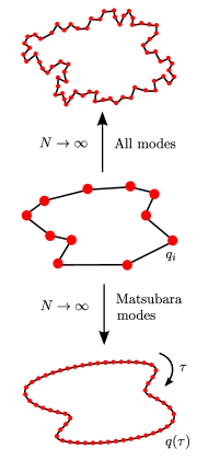
Figure 2: Schematic diagram showing that superpositions of Matsubara modes give distributions of path-integral coordinates $q_{l}$ which are smooth, differentiable functions of imaginary time $\tau$. Inclusion of non-Matsubara modes gives jagged distributions.

Matsubara modes have a long historyceperley ; charu ; doll ; char_cep in path-integral descriptions of equilibrium properties, since they give rise to an alternative ring-polymer expression for $C_{AB}(0)$. If we define

$$C_{AB}^{[M]}(0)={\alpha_{M}\over 2\pi\hbar}\int d{\bf\widetilde{P}} \int d{\bf\widetilde{Q}}\ A({\bf\widetilde{Q}})B({\bf\widetilde{Q}})e^{-\beta\widetilde{R}_{M}({\bf\widetilde{P}},{\bf\widetilde{Q}})}$$ (70)

with

$$\widetilde{R}_{M}({\bf\widetilde{P}},{\bf\widetilde{Q}})= \left(\sum_{n=-(M-1)/2}^{(M-1)/2}{{\widetilde{P}}_{n}^{2}\over 2m}+{m\over 2}\widetilde{\omega}_{n}^{2}\widetilde{Q}_{n}^{2}\right)+\widetilde{U}_{M}({\bf\widetilde{Q}})$$ (71)

$${\widetilde{U}}_{M}({\bf{\widetilde{Q}}})= \lim_{N\to\infty}{1\over N}\sum_{l=1}^{N}V\left(\sum_{n=-(M-1)/2}^{(M-1)/2}{T}_{ln}\sqrt{N}{\widetilde{Q}}_{n}\right)$$ (72)

$$\alpha_{M}= \hbar^{(1-M)}\left[(M-1)/2\right]!^{2}$$ (73)

then

$$C_{AB}(0)=\lim_{\begin{subarray}{c}M\to\infty\\ M\ll N\end{subarray}}C_{AB}^{[M]}(0)$$ (74)

where this limit indicates that $M$ is allowed to tend to infinity, subject to the condition that it is always much smaller than $N$, such that the ${\bf\widetilde{Q}}$ remain Matsubara modes. In practice, a good approximation to the exact result is reached once $\widetilde{\omega}_{(M-1)/2}$ exceeds the highest frequency in the potential $V(q)$. Equation (70) is less often used nowadays to compute static properties, because the convergence with respect to $M$ is typically slower than the convergence of Eq. (16) with respect to $N$.char_cep

However, Eq. (70) tells us something interesting: The Boltzmann factor ensures that only smooth distributions of $({\bf p},{\bf q})$ survive in $C_{AB}(t)$ at $t=0$; but at $t>0$, the force terms in ${\cal L}_{N}$ [Eq. (66)] will, in general, mix in an increasing proportion of non-smooth, non-Matsubara modes, so that the distributions of $({\bf p},{\bf q})$ become increasingly jagged as time evolves. The rate at which this mixing occurs depends on the anharmonicity of the potential $V(q)$. In the special case that $V(q)$ is harmonic, there is no coupling between different normal modes, so the distributions in $({\bf p},{\bf q})$ remain smooth for all time. In other words, smooth distributions in $({\bf p},{\bf q})$ are found in two of the limits (zero-time and harmonic) in which the LSC-IVR is known to be exact.

IV Matsubara dynamics

IV.1 Definition

The results of Sec. IIIC suggest that there may be a connection between smoothness in imaginary time and classical dynamics. We now investigate what happens if we constrain an initially smooth function of phase space coordinates $({\bf p},{\bf q})$ to remain smooth for all (real) times $t>0$. We take the (exact) quantum Liouvillian ${\hat{L}}_{N}$, and instead of truncating at $\hbar^{0}$ as in Eq. (66) (which gives the LSC-IVR), we retain all powers of $\hbar^{2}$, take the $N\to\infty$ limit, and split ${\hat{L}}_{N}$ into

$$\lim_{N\to\infty}{\hat{L}}_{N}={\cal L}_{M}+\lim_{N\to\infty}{\hat{L}}_{\rm error}(N,M)$$ (75)

where the ‘Matsubara Liouvillian’

$${\cal L}_{M}= \lim_{N\to\infty}\sum_{n=-(M-1)/2}^{(M-1)/2}{P_{n}\over m}{\partial\over\partial Q_{n}}$$

$$-U_{N}({\bf Q})\frac{2}{\hbar}\sin\!\left(\sum_{n=-(M-1)/2}^{(M-1)/2}\frac{\hbar}{2}{\overleftarrow{\partial}\over\partial Q_{n}}{\overrightarrow{\partial}\over\partial P_{n}}\right)$$ (76)

contains all terms in which the derivatives involve only the Matsubara modes, and ${\hat{L}}_{\rm error}(N,M)$ contains the rest of the terms (given in Appendix B). We then discard ${\hat{L}}_{\rm error}(N,M)$, approximating ${\hat{L}}_{N}$ by ${\cal L}_{M}$. We will refer to the (approximate) dynamics generated by ${\cal L}_{M}$ as ‘Matsubara dynamics’. By construction, Matsubara dynamics ensures that a distribution of $({\bf p},{\bf q})$ which is a smooth and differentiable function of $\tau$ at $t=0$ will remain so for all $t>0$.

The time-correlation function corresponding to Matsubara dynamics is

$$C_{AB}^{[M]}(t)= \lim_{N\rightarrow\infty}{1\over(2\pi\hbar)^{N}}\int d{\bf P}\int d{\bf Q}$$

$$\times\left[e^{-\beta{\hat{H}}}{\hat{A}}\right]_{\overline{N}}e^{{\cal L}_{M}t}\left[{\hat{B}}(0)\right]_{N}$$ (77)

We can obtain an explicit form for $C_{AB}^{[M]}(t)$ by taking the same limit as in Eq. (74), allowing $M$ to tend to infinity, subject to $M\ll N$, which gives (see Appendix C)

$$C_{AB}^{\rm Mats}(t)=\lim_{\begin{subarray}{c}M\to\infty\\ M\ll N\end{subarray}}C_{AB}^{[M]}(t)$$ (78)

where

$$C_{AB}^{[M]}(t)={\alpha_{M}\over 2\pi\hbar}\int d{\bf\widetilde{P}} \int d{\bf\widetilde{Q}}\ A({\bf\widetilde{Q}})e^{-\beta[{\widetilde{H}}_{M}({\bf\widetilde{P}},{\bf\widetilde{Q}})-i\theta_{M}({\bf\widetilde{P}},{\bf\widetilde{Q}})]}$$

$$\times e^{{\cal L}_{M}t}B({\bf\widetilde{Q}})$$ (79)

in which the Matsubara Hamiltonian is

$${\widetilde{H}}_{M}({\bf\widetilde{P}},{\bf\widetilde{Q}})={{\bf\widetilde{P}}^{2}\over 2m}+{\widetilde{U}}_{M}({\bf\widetilde{Q}})$$ (80)

and the phase factor is

$$\theta_{M}({\bf\widetilde{P}},{\bf\widetilde{Q}})=\sum_{n=-(M-1)/2}^{(M-1)/2}{\widetilde{P}}_{n}{\widetilde{\omega}}_{n}{\widetilde{Q}}_{-n}$$ (81)

with $\alpha_{M}$, $\widetilde{\omega}_{n}$, ${\bf\widetilde{P}}$ and ${\bf\widetilde{Q}}$ defined in Sec. IIIC. Note that, in deriving these equations (in Appendix C), we have not proved that $C_{AB}^{[M]}(t)$ converges with $M$ for $t>0$ (only that the form of Eqs. (79)-(81) converges with $M$). We test this convergence numerically in Sec. V.

Thus when the exact dynamics is approximated by Matsubara dynamics, the quantum Boltzmann distribution takes the simple form of a classical Boltzmann distribution multiplied by a phase factor. At $t=0$, one may analytically continue the phase factor (by making $P_{n}\to P_{n}-im\omega_{n}Q_{-n}$) to recover the ring-polymer distribution in Eq. (70). However, it is not known whether this analytic continuation is valid at $t>0$ (except for the special case of the harmonic oscillator), and hence the most general form of quantum Boltzmann distribution (in the space of Matsubara modes) is the one given in Eq. (79).

IV.2 Matsubara dynamics is classical

We now rewrite ${\cal L}_{M}$ in terms of $({\bf\widetilde{P}},{\bf\widetilde{Q}})$, to make explicit its dependence on $N$, and we also assume that $M$ is sufficiently large that Eq. (79) holds, allowing us to replace ${U}_{N}({\bf{Q}})/N$ by ${\widetilde{U}}_{M}({\bf{\widetilde{Q}}})$. This gives

$${\cal L}_{M}=\lim_{N\to\infty}{1\over m}{\bf{\widetilde{P}}}\cdot{\bf\nabla_{\widetilde{Q}}}-{\widetilde{U}}_{M}({\bf{\widetilde{Q}}})\frac{2N}{\hbar}\sin\!\left(\frac{\hbar}{2N}\ {{\bf{\overleftarrow{\nabla}}_{\widetilde{Q}}}}\cdot{{\bf{\overrightarrow{\nabla}}_{\widetilde{P}}}}\right).$$ (82)

In other words, the Moyal series in Matsubara spacearti2 is an expansion in terms of $(\hbar/N)^{2}$, rather than $\hbar^{2}$. Now, it is well knownheller that the smallness of $\hbar$ cannot in general be used to justify truncating the (standard LSC-IVR) Moyal series of Eq. (30) at $\hbar^{0}$, since at least one of the Wigner transforms in the time-correlation function [Eq. (23)] contains derivatives that scale as $\hbar^{-1}$. However, it is easy to show that the derivatives of all terms in the integral in Eq. (79) scale as $N^{0}$. As a result, it follows that all derivatives higher than first order in ${\cal L}_{M}$ vanish in the limit $N\to\infty$, with the result that

$${\cal L}_{M}=\sum_{n=-(M-1)/2}^{(M-1)/2}{{\widetilde{P}}_{n}\over m}{\partial\over\partial{\widetilde{Q}}_{n}}-{\partial{\widetilde{U}}_{M}({\bf\widetilde{Q}})\over\partial{\widetilde{Q}}_{n}}{\partial\over\partial{\widetilde{P}}_{n}}$$ (83)

In other words, Matsubara dynamics is classical.

This is a surprising result, which needs to be interpreted with caution. It does not mean that the dependence of $B({\bf Q})$ on the Matsubara modes evolves classically in the exact quantum dynamics, since the exact Liouvillian ${\hat{L}}_{N}$ contains derivative terms that couple the Matsubara modes with the non-Matsubara modes (for which the higher-order derivatives cannot be neglected): it means that the dynamics of the Matsubara modes becomes classical when they are decoupled from the non-Matsubara modes.

One way to understand the origin of the $\hbar/N$ in Eq. (82) is to note that the Fourier transform between ${\widetilde{P}}_{n}$ and ${\widetilde{D}}_{n}$ (in the Wigner transforms of Eqs. (42) and (43)) is $\exp(iN{\widetilde{P}}_{n}{\widetilde{D}}_{n}/\hbar)$. Hence the effective Planck’s constant associated with motion in the Matsubara coordinates tends to zero in the limit $N\to\infty$. Note that the dependence of the Boltzmann distribution on the non-Matsubara modes is more complicated than that of Eq. (79), and contains powers of $(\hbar/N)^{-1}$ which cancel out the powers of $(\hbar/N)$ in ${\hat{L}}_{N}$ (which must obviously happen, since we know that the exact dynamics is not in general classical).

Matsubara dynamics thus has many features in common with LSC-IVR: it is exact in the $t=0$ limit (when all distributions of $({\bf p},{\bf q})$ are smooth superpositions of Matsubara modes), in the harmonic limit (where the dynamics of the Matsubara modes is decoupled from that of the non-Matsubara modes), and in the classical limit (since setting $M=0$ in Eq. (79) gives the classical time-correlation function); and it neglects all terms ${\cal O}(\hbar^{2})$ in the (exact) quantum Liouvillian. However, Matsubara dynamics differs from LSC-IVR in that it also neglects the terms ${\cal O}(\hbar^{0})$ that contain derivatives in the non-Matsubara modes. One can thus regard Matsubara dynamics as a filtered version of LSC-IVR, in which the parts of the dynamics that cause the smooth distributions of $({\bf p},{\bf q})$ to become jagged have been removed.der2

IV.3 Conservation of the quantum Boltzmann distribution

Confining the dynamics to the space of Matsubara modes has a major effect on the symmetry of the Hamiltonian. The LSC-IVR Hamiltonian ${H}_{N}({\bf P},{\bf Q})$ is simply the classical Hamiltonian of $N$ independent particles, and is thus symmetric with respect to any permutation of the phase space coordinates [e.g. $(p_{1},q_{1})\leftrightarrow(p_{3},q_{3})$]. On restricting the dynamics to the Matsubara modes, most of these symmetries are lost (since individual permutations would destroy the smoothness of the distributions of $({\bf p},{\bf q})$). However, one operation which is retainedreflect is symmetry with respect to cyclic permutation of the coordinates, which, on restricting the dynamics to Matsubara space, becomes a continuous, differentiable symmetry, namely invariance with respect to translation in imaginary time:

$${d{\widetilde{H}}_{M}({\bf\widetilde{P}},{\bf\widetilde{Q}})\over d\tau}=0$$ (84)

(see Appendix A). It thus follows from Noether’s theorem,goldstein that

$${d\widetilde{\Lambda}_{M}({\bf\widetilde{P}},{\bf\widetilde{Q}})\over d\tau}={d\over dt}\left(\sum_{n=-(M-1)/2}^{(M-1)/2}{\widetilde{P}}_{n}{d{\widetilde{Q}}_{n}\over d\tau}\right)=0$$ (85)

where $\Lambda_{M}({\bf\widetilde{P}},{\bf\widetilde{Q}})$ is the Matsubara Lagrangian. In other words, in Matsubara dynamics, there exists a constant of the motion (in addition to the total energy) which is given by the term in brackets above.

In Appendix A, it is shown that the phase $\theta_{M}({\bf\widetilde{P}},{\bf\widetilde{Q}})$ in the quantum Boltzmann distribution [Eqs. (79)-(81)] can be written

$$\theta_{M}({\bf\widetilde{P}},{\bf\widetilde{Q}})=-\!\!\!\!\!\!\!\sum_{n=-(M-1)/2}^{(M-1)/2}{\widetilde{P}}_{n}{d{\widetilde{Q}}_{n}\over d\tau}$$ (86)

and is thus the constant of the motion associated with the invariance of ${\widetilde{H}}_{M}({\bf\widetilde{P}},{\bf\widetilde{Q}})$ to imaginary time-translation. Since ${\widetilde{H}}_{M}({\bf\widetilde{P}},{\bf\widetilde{Q}})$ is of course also a constant of the motion, it follows that Matsubara dynamics conserves the quantum Boltzmann distribution.

As a result, Matsubara dynamics satisfies the detailed balance relation

$$C_{AB}^{[M]}(t)=C_{BA}^{[M]}(-t)$$ (87)

and gives expectation values

$$\big{<}{\hat{B}}\big{>}^{[M]}(t)= {\alpha_{M}\over 2\pi\hbar}\int d{\bf\widetilde{P}}\int d{\bf\widetilde{Q}}$$

$$\times e^{-\beta[{\widetilde{H}}_{M}({\bf\widetilde{P}},{\bf\widetilde{Q}})-i\theta_{M}({\bf\widetilde{P}},{\bf\widetilde{Q}})]}B({\bf\widetilde{Q}}_{t})$$

$$= {\alpha_{M}\over 2\pi\hbar}\int d{\bf\widetilde{P}}_{t}\int d{\bf\widetilde{Q}}_{t}$$

$$\times e^{-\beta[{\widetilde{H}}_{M}({\bf\widetilde{P}}_{t},{\bf\widetilde{Q}}_{t})-i\theta_{M}({\bf\widetilde{P}}_{t},{\bf\widetilde{Q}}_{t})]}B({\bf\widetilde{Q}}_{t})$$

$$= {\alpha_{M}\over 2\pi\hbar}\int d{\bf\widetilde{P}}_{t}\int d{\bf\widetilde{Q}}_{t}$$

$$\times e^{-\beta{\widetilde{R}}_{M}({\bf\widetilde{P}}_{t},{\bf\widetilde{Q}}_{t})}B({\bf\widetilde{Q}}_{t})$$

$$= \big{<}{\hat{B}}\big{>}^{[M]}(0)$$ (88)

which are independent of time (and equal to the exact quantum result in the limit $M\to\infty$; see Eq. (74)). Note that the step between the second and third lines follows from analytic continuation ($P_{n}\to P_{n}-im\omega_{n}Q_{-n}$).

We thus have the surprising result that a purely classical dynamics (Matsubara dynamics) which uses the smoothed Hamiltonian that arises naturally when the space is restricted to Matsubara modes, conserves the quantum Boltzmann distribution. At first sight this may appear counter-intuitive. For example, it is clear that the classical dynamics will not respect zero-point energy constraints, nor will it be capable of tunnelling. However, it is the phase $\theta_{M}({\bf\widetilde{P}},{\bf\widetilde{Q}})$ which converts what would otherwise be a classical Boltzmann distribution in an extended phase-space into a quantum Boltzmann distribution, and the phase is conserved.

IV.4 Generalizations

The derivations above can easily be generalized to systems with any number of dimensions. For a system whose classical Hamiltonian resembles Eq. (2), there are $F\times M$ Matsubara modes, one set of $M$ modes in each dimension. All the steps in Secs. III and IV.A-C are then the same, except that, with $F$ dimensions instead of one, there is now a sum of $F$ phase terms, each resembling $\theta_{M}({\bf\widetilde{P}},{\bf\widetilde{Q}})$. Noether’s theorem shows that the sum of these terms and hence the quantum Boltzmann distribution is conserved.

We emphasise that the derivations above were carried out for operators ${\hat{A}}$ and ${\hat{B}}$ in $C_{AB}(t)$ which are general functions of the coordinate operators ${\hat{q}}$. Matsubara dynamics is therefore not limited to correlation functions involving linear operators of position. The derivations can also be repeated, with minor modifications in the algebra, for the case that ${\hat{A}}$ and ${\hat{B}}$ are general functions of the momentum operator (which results in functions of ${\bf\widetilde{P}}$ appearing in the generalised Wigner transforms).

V Numerical tests of the efficacy of Matsubara dynamics

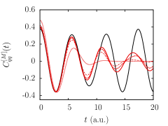
Figure 3: Convergence with respect to number of modes $M$ of the Matsubara position auto-correlation function $C_{qq}^{[M]}(t)$, calculated for the quartic potential of Eq. (89), at a reciprocal temperature of $\beta=2$ a.u. The red lines correspond to $M=1$ (dots), 3 (chains), 5 (dashes) and 7 (solid). The solid black line is the exact quantum result.

Figure 4: Evolution of the phase $\theta_{M}({\bf\widetilde{P}},{\bf\widetilde{Q}})$ along a single classical trajectory on the quartic potential, with $M=5$, and $N=5$ (dots), 9 (dashes) and $\infty$ (solid line). The latter corresponds to Matsubara dynamics in which the phase is conserved.

So far we have made no attempt to justify the use of Matsubara dynamics, beyond pointing out that it is exact in all the limits in which LSC-IVR is exact, but that, unlike LSC-IVR, it also conserves the quantum Boltzmann distribution. Here we investigate whether Matsubara dynamics converges with respect to the number of modes $M$, and make numerical comparisons with the LSC-IVR, CMD and RPMD methods.

The presence of the phase $\theta_{M}({\bf\widetilde{P}},{\bf\widetilde{Q}})$ in the Boltzmann distribution [Eq. (79)] means that Matsubara dynamics suffers from the sign problem, and thus cannot be used as a practical method. However, we were able to evaluate $C_{qq}^{[M]}(t)$ (i.e. $C_{AB}^{[M]}(t)$ of Eq. (79) with ${\hat{A}}=\hat{q}$, ${\hat{B}}=\hat{q}$) for some one-dimensional model systems. For consistency with previous work,craig1 ; rossky we considered the quartic potential

$$V(q)=\frac{1}{4}q^{4}$$ (89)

and the weakly anharmonic potential

$$V(q)=\frac{1}{2}q^{2}+\frac{1}{10}q^{3}+\frac{1}{100}q^{4}$$ (90)

where atomic units are used with $m=1$. Calculations using potentials with intermediate levels of anharmonicity were found to give similar results (and are not shown here).

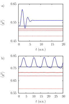
Figure 5: Time-dependence of the thermal expectation value $\big{<}q^{2}\big{>}(t)$ for the quartic potential at $\beta=2$, computed using LSC-IVR (blue), and Matsubara dynamics (red: $M=1$ (dots), 3 (dashes), 5 (solid)), and compared with the exact quantum result (black).

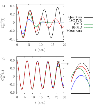
Figure 6: Comparisons of position-autocorrelation functions computed using different levels of theory, for (a) the quartic potential and (b) the weakly anharmonic potential of Eq. (90). The Matsubara results were obtained using $M=7$ (quartic) and $M=5$ (weakly anharmonic).

Figure 3 shows $C_{qq}^{[M]}(t)$ for the quartic potential, at an inverse temperature of $\beta=2$ a.u., for various values of $M$. These results were obtained by propagating classical trajectories using the Matsubara potential ${\widetilde{U}}_{M}({\bf\widetilde{Q}})$ to generate the forces, subject to the Anderson thermostatdaan (according to which each $\widetilde{P}_{n}$ was reassigned to a value drawn at random from the classical Boltzmann distribution every 2 atomic time units); ${\widetilde{U}}_{M}({\bf\widetilde{Q}})$ was computed by taking the $N\to\infty$ limit analytically, as described in the supplemental material.suppl A total of $10^{11}$ Monte Carlo points was found necessary to converge $C_{qq}^{[M]}(t)$. Extending these calculations beyond $M=7$ was prohibitively expensive, and the final few $M$ were particularly difficult to converge (since $\theta_{M}({\bf\widetilde{P}},{\bf\widetilde{Q}})$ becomes increasingly oscillatory as $\widetilde{\omega}_{n}$ increases). Nevertheless, the results in Fig. 3 are sufficient to show that $C_{qq}^{[M]}(t)$ converges with respect to $M$, although the convergence appears to become slower as $t$ increases. For the weakly anharmonic potential, convergence to within graphical accuracy was obtained using $M=5$ for $\beta=2$ a.u.

We also confirmed numerically that Matsubara dynamics conserves the quantum Boltzmann distribution. Figure 4 shows the phase $\theta_{M}({\bf\widetilde{P}},{\bf\widetilde{Q}})$ as a function of time along a Matsubara trajectory. When a coarse number of polymer beads ($N=5$) is used, such that the $M$ lowest-frequency modes are a poor approximation to the Matsubara modes, the phase is not conserved; however, as $N$ is increased, the variation of the phase along the trajectory flattens, becoming completely time-independent in the limit $N\to\infty$. Figure 5 plots the expectation value $\big{<}q^{2}\big{>}^{[M]}(t)$, which is found to be time-independent as expected from Eq. (88).

Figure 6 compares the Matsubara correlation functions $C_{qq}^{[M]}(t)$ for both potentials with exact quantum, LSC-IVR, CMD and RPMD results. The quartic potential at $\beta=2$ (panel a) is a severe test for which any method that neglects real-time coherence fails after a single recurrence. Nevertheless, we see that Matsubara dynamics gives a much better treatment than LSC-IVR, reproducing almost perfectly the first recurrence at 6 a.u., and damping to zero more slowly.sc-ivr The Matsubara result is also better than both the CMD and RPMD results. The same trends are found for the weakly anharmonic potential (Fig. 6, panel b), and were also found for the potentials with intermediate anharmonicity (not shown).

VI Conclusions

We have found that a single change in the derivation of LSC-IVR dynamics gives rise to a classical dynamics (‘Matsubara dynamics’) which preserves the quantum Boltzmann distribution. This change involves no explicit truncation in powers of $\hbar^{2}$, but instead a decoupling of a subspace of ring-polymer normal modes (the Matsubara modes) from the other modes. The dynamics in this restricted space is found to be purely classical and to ensure that smooth distributions of phase-space points (as a function of imaginary time), which are present in the Boltzmann distribution at time $t=0$, remain smooth at all later times. The LSC-IVR dynamics, by contrast, includes all the modes, which has the effect of breaking up these smooth distributions, and thus failing to preserve the quantum Boltzmann distribution. Numerical tests show that Matsubara dynamics gives consistently better agreement than LSC-IVR with the exact quantum time-correlation functions.

These results suggest that Matsubara dynamics is a better way than LSC-IVR, at least in principle, to account for the classical mechanics in quantum time-correlation functions. We suspect that Matsubara dynamics may be equivalent to expanding the time-dependence of the quantum time-correlation function in powers of $\hbar^{2}$ and truncating it at $\hbar^{0}$; this is in contrast to LSC-IVR, in which one truncates the quantum Liouvillianhigh at $\hbar^{0}$. However, further work will be needed to prove or disprove this conjecture.

Matsubara dynamics is far too expensive to be useful as a practical method. However, it is probably a good starting point from which to make further approximations in order to develop such methods. The numerical tests reported here show that Matsubara dynamics gives consistently better results than both CMD and RPMD, suggesting that these popular methods may be approximations to Matsubara dynamics.

Appendix A Differentiability with respect to imaginary time

A distribution of ring-polymer coordinates $q_{l},\,l=1,\dots,N$, can be written as a smooth and differentiable function of the imaginary time $\tau$ ($0\leq\tau<\beta\hbar$) if the limit

$${dq(\tau)\over d\tau}=\lim_{N\to\infty}{q_{l+1}-q_{l-1}\over 2\beta_{N}\hbar},\quad\tau=l\hbar\beta_{N}$$ (91)

exists, i.e. if

$$\lim_{N\to\infty}q_{l+1}-q_{l-1}\sim N^{-1}$$ (92)

For a distribution formed by superposing only the Matsubara modes, we can use trigonometric identities and the definitions in Sec. III to write

$$q_{l+1}-q_{l-1}$$

$$=2\sqrt{2}\sum_{n=1}^{(M-1)/2}\left[\cos\left({2\pi nl\over N}\right){\widetilde{Q}}_{n}-\sin\left({2\pi nl\over N}\right){\widetilde{Q}}_{-n}\right]$$

$$\ \ \ \times\sin\left({2\pi n\over N}\right)$$ (93)

Since $n\ll N$, the sine function on the right ensures that Eq. (92) is satisfied; also, repetition of this procedure shows that higher-order differences of order $\lambda$ scale as $N^{-\lambda}$. Hence a distribution $q_{l}$ formed from a superposition of Matsubara modes is a smooth and differentiable function of $\tau$. The same is true for distributions in $p_{l}$ and $\Delta_{l}$.

To prove that the Matsubara Hamiltonian is invariant under imaginary-time translation [Eq. (84)], we first differentiate the Matsubara potential $U_{M}({\bf\widetilde{Q}})$ with respect to $\tau$, which gives

$${d\widetilde{U}_{M}({\bf\widetilde{Q}})\over d\tau}=\lim_{N\to\infty}{\widetilde{\cal P}_{1}\,\widetilde{U}_{M}({\bf q})-\widetilde{U}_{M}({\bf q})\over\beta_{N}\hbar}$$ (94)

where

$$\widetilde{U}_{M}({\bf q})=\sum_{l=1}^{N}V\left(\sum_{m=1}^{N}\ \sum_{n=-(M-1)/2}^{(M-1)/2}T_{ln}T_{mn}q_{m}\right)$$ (95)

and ${\cal P}_{1}$ represents a cyclic permutation of the coordinates $q_{m}\to q_{m+1}$, such that

$${\cal P}_{1}\,\widetilde{U}_{M}({\bf q})=\sum_{l=1}^{N}V\left(\sum_{m=1}^{N}\ \sum_{n=-(M-1)/2}^{(M-1)/2}T_{ln}T_{(m-1)\,n}q_{m}\right)$$ (96)

We then rearrange the sum over $n$ in Eq. (96) into

$$T_{l0}T_{(m-1)\,0}+\sum_{n=1}^{(M-1)/2}\left[T_{ln}T_{(m-1)\,n}+T_{l\,-n}T_{(m-1)\,-n}\right]$$ (97)

and use trigonometric identities to show that

$$T_{ln}T_{(m-1)\,n}+T_{l\,-n}T_{(m-1)\,-n}$$

$$=T_{(l+1)\,n}T_{mn}+T_{(l+1)\,-n}T_{m\,-n}$$ (98)

Re-ordering the sum over $l$ and using the property that $T_{l0}=N^{-1/2}$ gives

$${\cal P}_{1}\,\widetilde{U}_{M}({\bf q})=\widetilde{U}_{M}({\bf q})$$ (99)

which proves that

$${d\widetilde{U}_{M}({\bf\widetilde{Q}})\over d\tau}=0$$ (100)

The same line of argument can be applied to the kinetic energy ${\bf\widetilde{P}}^{2}/2m$, thus proving Eq. (84).

To obtain the derivative of $\widetilde{Q}_{n}$ with respect to $\tau$ (needed to prove Eq. (86)), we write

$${d\widetilde{Q}_{n}\over d\tau}= \lim_{N\to\infty}{1\over\sqrt{N}}\sum_{l=1}^{N}T_{ln}{q_{l+1}-q_{l-1}\over 2\beta_{N}\hbar}$$

$$= \lim_{N\to\infty}{1\over\sqrt{N}}\sum_{l=1}^{N}{[T_{(l-1)\,n}-T_{(l+1)\,n}]q_{l}\over 2\beta_{N}\hbar}$$ (101)

and use trigonometric identities to obtain

$$T_{l+1\,n}-T_{l-1\,n}=2T_{l\,-n}\sin(2n\pi/N)$$ (102)

Since $n\ll N$, it follows that

$${d\widetilde{Q}_{n}\over d\tau}=-{\widetilde{\omega}}_{n}\widetilde{Q}_{-n}$$ (103)

where $\widetilde{\omega}_{n}$ is the Matsubara frequency defined in Eq. (67).

Appendix B Error term for Matsubara Liouvillian

The error term ${\hat{L}}_{\rm error}(N,M)$ of Eq. (75) is the difference ${\hat{L}}_{N}-{\cal L}_{M}$ between the exact quantum Liouvillian and the Matsubara Liouvillian. Using Eqs. (65) and (76) and the trigonometric identity

$$\sin(a+b)-\sin a\equiv 2\sin\left({b\over 2}\right)\cos\left(a+{b\over 2}\right)$$ (104)

we can write

$${\hat{L}}_{\rm error}(N,M)= \sum_{n=(M+1)/2}^{(N-1)/2}\frac{P_{-n}}{m}\frac{\partial}{\partial Q_{-n}}+\frac{P_{n}}{m}\frac{\partial}{\partial Q_{n}}$$

$$-\frac{4}{\hbar}U({\bf Q})\sin\!\left({{\hat{X}}\over 2}\right)\cos\!\left({\hat{Y}}+{{\hat{X}}\over 2}\right)$$ (105)

with

$${\hat{X}}={\hbar\over 2}\sum_{n=(M+1)/2}^{(N-1)/2}\frac{\overleftarrow{\partial}}{\partial Q_{-n}}\frac{\overrightarrow{\partial}}{\partial P_{-n}}+\frac{\overleftarrow{\partial}}{\partial Q_{n}}\frac{\overrightarrow{\partial}}{\partial P_{n}}$$ (106)

and

$${\hat{Y}}={\hbar\over 2}\sum_{n=-(M-1)/2}^{(M-1)/2}\frac{\overleftarrow{\partial}}{\partial Q_{n}}\frac{\overrightarrow{\partial}}{\partial P_{n}}$$ (107)

Appendix C Derivation of Matsubara time-correlation function

To obtain the expression for $C_{AB}^{[M]}(t)$ in Eq. (79), we note that $B({\bf P},{\bf Q},t)$ is independent of the non-Matsubara ${\bf P}$ modes (since, by construction, these modes are not involved in the Matsubara dynamics) which can therefore be integrated out, giving a product of Dirac delta-functions in the non-Matsubara ${\bf\widetilde{D}}$ modes.pnote As a result, the Wigner transform $\left[e^{-\beta{\hat{H}}}{\hat{A}}\right]_{\overline{N}}$ in Eq. (77) reduces to

$$\left[e^{-\beta{\hat{H}}}{\hat{A}}\right]_{\overline{N}}({\bf P}_{M},{\bf Q})$$

$$=(2\pi\hbar)^{N-M}A({\bf Q})\int d{\bf D}_{M}\prod_{n=-(M-1)/2}^{(M-1)/2}e^{i{P}_{n}D_{n}/\hbar}$$

$$\ \ \ \times\prod_{l=1}^{N}\langle\eta^{-}_{l-1}({\bf Q},{\bf D}_{M})|e^{-\beta_{N}\hat{H}}|\eta^{+}_{l}({\bf Q},{\bf D}_{M})\rangle$$ (108)

where ${\bf P}_{M}$ and ${\bf D}_{M}$ include only the Matsubara modes (and ${\bf Q}$ includes all $N$ modes), and

$$\eta^{\pm}_{l}({\bf Q},{\bf D}_{M})=\sum_{n=-(N-1)/2}^{(N-1)/2}T_{ln}Q_{n}\pm\sum_{n=-(M-1)/2}^{(M-1)/2}T_{ln}D_{n}/2$$ (109)

(where the dependence of $\eta^{\pm}_{l}$ on $({\bf Q},{\bf D}_{M})$ will be suppressed in what follows). Expressing the bra-ket in ring-polymer form, and using trigonometric identities, we obtain

$$\left[e^{-\beta{\hat{H}}}{\hat{A}}\right]_{\overline{N}}({\bf P}_{M},{\bf Q})$$

$$=(2\pi\hbar)^{N-M}\left({m\over 2\pi\beta_{N}\hbar^{2}}\right)^{N/2}A({\bf Q})\int d{\bf D}_{M}$$

$$\ \ \ \times e^{-\beta_{N}mf_{M}({\bf Q},{\bf D}_{M})/2}\prod_{n=-(M-1)/2}^{(M-1)/2}e^{i{P}_{n}D_{n}/\hbar}$$

$$\ \ \ \times\exp\left\{-{\beta_{N}\over 2}\left[\sum_{l=1}^{N}V(\eta^{-}_{l})+V(\eta^{+}_{l})\right]\right\}$$ (110)

where

$$f_{M}({\bf Q},{\bf D}_{M})$$

$$={4\over(\beta_{N}\hbar)^{2}}\sum_{n=-(M-1)/2}^{(M-1)/2}\left(Q_{n}\sin{n\pi\over N}+{D_{-n}\over 2}\cos{n\pi\over N}\right)^{2}$$

$$\ \ \ +\sum_{n=(M+1)/2}^{(N-1)/2}(Q_{n}^{2}+Q_{-n}^{2})\omega_{n}^{2}$$ (111)

On taking the limit $N\to\infty$, and converting ${\bf D}_{M}$ to ${\bf\widetilde{D}}$, we find that the Gaussians involving ${\bf D}_{M}$ in Eq. (110) have the form

$$\exp\left(-m{\widetilde{D}}_{n}^{2}N^{2}/2\beta\hbar^{2}\right)$$ (112)

i.e. each Gaussian in ${\bf\widetilde{D}}$ becomes a Dirac delta-function in the limit $N\to\infty$. This allows us to replace the third line in Eq. (110) by

$$\exp\left[-\beta_{N}\sum_{l=1}^{N}V\left(\sum_{n=-(N-1)/2}^{(N-1)/2}T_{ln}Q_{n}\right)\right]$$ (113)

and to integrate out the ${\bf\widetilde{D}}$, giving

$$\left[e^{-\beta{\hat{H}}}{\hat{A}}\right]_{\overline{N}}({\bf P}_{M},{\bf Q})$$

$$=\left({2\pi m\over\beta_{N}}\right)^{(N-M)/2}A({\bf Q})$$

$$\ \ \ \times e^{-\beta_{N}{\bf P}_{M}^{2}/2m}\prod_{n=-(M-1)/2}^{(M-1)/2}e^{2i{P}_{n}{Q}_{-n}\tan(n\pi/N)/\hbar}$$

$$\ \ \ \times\exp\left[-{\beta_{N}\over 2}\sum_{l=1}^{N}V\left(\sum_{n=-(N-1)/2}^{(N-1)/2}T_{ln}Q_{n}\right)\right]$$

$$\ \ \ \times\exp\left[-{\beta_{N}m\over 2}\sum_{n=(M+1)/2}^{(N-1)/2}(Q_{n}^{2}+Q_{-n}^{2})\omega_{n}^{2}\right]$$ (114)

We then substitute this expression into the integral of Eq. (77) (with $\int d{\bf P}$ replaced by $\int d{\bf P}_{M}$), and take the limit $M\to\infty$ (subject to $M\ll N$), which allows us to integrate out the non-Matsubara modes in ${\bf Q}$. Use of the formulagrad

$$\prod_{n=1}^{N-1}\sin\left(n\pi/N\right)={N/2^{N-1}}$$ (115)

then gives Eqs. (79)-(81).

References

- (1) D. Chandler, Introduction to Modern Statistical Mechanics (Oxford University Press, New York, 1987).
- (2) D. Frenkel and B. Smit, Understanding Molecular Simulation (Academic Press, London, 2002).
- (3) J. Liu, W.H. Miller, F. Paesani, W. Zhang and D.A. Case, J. Chem. Phys. 131, 164509 (2009).
- (4) S.D. Ivanov, A Witt, M. Shiga and D. Marx, J. Chem. Phys. 132, 031101 (2010).
- (5) S. Habershon, G.S. Fanourgakis and D.E. Manolopoulos, J. Chem. Phys. 129, 074501 (2008).
- (6) E.M. McIntosh, K.T. Wikfeldt, J. Ellis, A. Michaelides and W. Allison, J. Phys. Chem. Lett. 4 1565 (2013).
- (7) Y.V. Suleimanov, J. Phys. Chem. A 116, 11141 (2012).
- (8) N. Boekelheide, R. Salomón-Ferrer and T.F. Miller III, PNAS 108, 16159 (2011).
- (9) R. Collepardo-Guevara, I.R. Craig and D.E. Manolopoulos, J. Chem. Phys. 128, 144502 (2008).
- (10) S. Hammes-Schiffer and A.A. Stuchebrukhov, Chem. Rev. 110, 6939 (2010).
- (11) M. Topaler and N. Makri, J. Chem. Phys. 101, 7500 (1994).
- (12) Q. Shi, L. Zhu and L. Chen, J. Chem. Phys. 135, 044505 (2011).
- (13) J.B. Rommel, T.P.M. Goumans and J. Kästner, J. Chem. Theor. Comput. 7, 690 (2011).
- (14) This definition of the time-correlation function (excluding the ) will be used throughout.
- (15) W.H. Miller, J. Phys. Chem. A 105, 2942 (2001).
- (16) H. Wang, X. Sun and W.H. Miller, J. Chem. Phys. 108, 9726 (1998).
- (17) Q. Shi and E. Geva, J. Chem. Phys. 118, 8173 (2003).
- (18) T. Yamamoto, H. Wang and W.H. Miller, J. Chem. Phys. 116, 7335 (2002).
- (19) J. Liu and W.H. Miller, J. Chem. Phys. 131, 074113 (2009).
- (20) J.A. Poulsen, G. Nyman and P.J. Rossky, J. Chem. Phys. 119, 12179 (2003).
- (21) Q. Shi and E. Geva, J. Phys. Chem. A 107, 9059 (2003).
- (22) J. Liu, “Recent advances in the linearized semiclassical initial value representation/classical Wigner model for the thermal correlation function,” Int. J. Quantum Chem. (published online).
- (23) J. Beutier, D. Borgis, R. Vuilleumier and S. Bonella, J. Chem. Phys. 141, 084102 (2014).
- (24) S. Bonella and D.F. Coker, J. Chem. Phys. 122, 194102 (2005).
- (25) P. Huo, T.F. Miller III and D.F. Coker, J. Chem. Phys. 139, 151103 (2013).
- (26) M. Hillery, R.F. O’Connell, M.O. Scully and E.P. Wigner, Phys. Rep. 106, 121 (1984).
- (27) E.J. Heller, J. Chem. Phys. 65, 1289 (1976).
- (28) J. Liu and W.H. Miller, J. Chem. Phys. 134, 104102 (2011).
- (29) J. Liu, J. Chem. Phys. 140, 224107 (2014).
- (30) J.A. Poulsen, personal communication (2014).
- (31) S. Jang and G.A. Voth, J. Chem. Phys. 111, 2371 (1999).
- (32) T.D. Hone, P.J. Rossky and G.A. Voth, J. Chem. Phys. 124, 154103 (2006).
- (33) I.R. Craig and D.E. Manolopoulos, J. Chem. Phys. 121, 3368 (2004).
- (34) I.R. Craig and D.E. Manolopoulos, J. Chem. Phys. 122, 084106 (2005).
- (35) I.R. Craig and D.E. Manolopoulos, J. Chem. Phys. 123, 034102 (2005).
- (36) T.E. Markland and D.E. Manolopoulos, J. Chem. Phys. 129, 024105 (2008).
- (37) S. Habershon, D.E. Manolopoulos, T.E. Markland and T.F. Miller III, Annu. Rev. Phys. Chem. 64, 387 (2013).
- (38) A.R. Menzeleev, N. Ananth and T.F. Miller III, J. Chem. Phys. 135, 074106 (2011).
- (39) J.S. Kretchmer and T.F. Miller III, J. Chem. Phys. 138, 134109 (2013).
- (40) A.R. Menzeleev, F. Bell and T.F. Miller III, J. Chem. Phys. 140, 064103 (2014).
- (41) N. Ananth, J. Chem. Phys. 139, 124102 (2013).
- (42) Y. Li, Y.V. Suleimanov, M. Yang, W.H. Green and H. Guo, J. Phys. Chem. Lett. 4, 48 (2013).
- (43) R. Pérez de Tudela, F.J. Aoiz, Y.V. Suleimanov and D.E. Manolopoulos, J. Phys. Chem. Lett. 3, 493 (2012).
- (44) Y.V. Suleimanov, W.J. Kong, H. Guo and W.H. Green, 141, 244103 (2014).
- (45) P.E. Videla, P.J. Rossky and D. Laria, J. Chem. Phys. 139, 174315 (2013).
- (46) M. Rossi, M. Ceriotti and D.E. Manolopoulos, J. Chem. Phys. 140, 234116 (2014).
- (47) J.O. Richardson and S.C. Althorpe, J. Chem. Phys. 131, 214106 (2009).
- (48) T.J.H. Hele and S.C. Althorpe, J. Chem. Phys. 138, 084108 (2013).
- (49) S.C. Althorpe and T.J.H. Hele, J. Chem. Phys. 139, 084115 (2013).
- (50) T.J.H. Hele and S.C. Althorpe, J. Chem. Phys. 139, 084116 (2013).
- (51) T.J.H. Hele, Quantum Transition-State Theory, PhD Thesis (University of Cambridge, 2014).
- (52) J.O. Richardson and M. Thoss, J. Chem. Phys. 139, 031102 (2013).
- (53) Y. Zhang, T. Stecher, M.T. Cvitas and S.C. Althorpe, J. Phys. Chem. Lett. 5, 3976 (2014).
- (54) R. Zwanzig, Nonequilibrium Statistical Mechanics, (Oxford University Press, New York, 2001).
- (55) D. Chandler and P.G. Wolynes, J. Chem. Phys. 74, 4078 (1981).
- (56) M. Parrinello and A. Rahman, J. Chem. Phys. 80, 860 (1984).
- (57) D.M. Ceperley, Rev. Mod. Phys. 67, 279 (1995).
- (58) C. Chakravarty, Int. Rev. Phys. Chem. 16, 421 (1997).
- (59) This paragraph is a heuristic summary of what is derived properly in refs. miller_molphys, and shi_geva, .
- (60) One could alternatively define the coordinates and such that has the form of and vice versa; this would yield identical results in the limit .
- (61) All the derivations reported here can also be done for even , at the cost of doubling the amount of algebra in order to deal with the awkward -th normal mode.
- (62) T. Matsubara, Prog. Theor. Phys. 14, 351 (1955).
- (63) Clearly this distinction is artificial, since, for any , there will be ‘non-Matsubara’ modes for which and , and which therefore also satisfy Eq. (67). However, all we need to know is that all of the Matsubara modes become increasingly smooth in the limit , and that the majority of the non-Matsubara modes do not.
- (64) D.L. Freeman and J.D. Doll, J. Chem. Phys. 80, 5709 (1984).
- (65) C. Chakravarty, M.C. Gordillo and D.M. Ceperley, J. Chem. Phys. 109, 2123 (1998).
- (66) The -dependence in Eq. (82) is not an artifact of having scaled to ; each derivative with respect to or in Eq. (76) carries an implicit scaling of .
- (67) We could thus have derived Matsubara dynamics by starting with the LSC-IVR Liouvillian of Eq. (66), then discarding the non-Matsubara derivative terms; but this would have hidden the important property that Matsubara dynamics is inherently classical.
- (68) Reflection symmetries (e.g. ) are also retained.
- (69) H. Goldstein, Classical Mechanics, 2nd ed. (Addison-Wesley, Reading, Massachusetts, 1980).
- (70) See supplemental material at [URL] for further details of these numerical calculations.
- (71) The persistence of the oscillations in the Matsubara result for the quartic oscillator (Fig. 6a) suggests that a Matsubara version of (non-linearized) semiclassical-IVR (i.e. the next approximation up in the hierarchy, in which individual forward-backward paths are treated classically and assigned phasesmiller_rev ) may give very close agreement with the exact quantum result for significantly longer times.
- (72) These two approximations are identical only in the limits in which LSC-IVR and Matsubara dynamics agree and are both exact (i.e. the short-time, harmonic and high-temperature limits).
- (73) Note that if is a function of the momentum operator, then does depend on the non-Matsubara coordinates, but that this dependence has a known, analytic, form, such that these coordinates can be integrated out, converting the original dependence on the non-Matsubara coordinates into a dependence on the non-Matsubara coordinates.
- (74) I.S. Gradshteyn and I.M. Ryzhik, Table of Integrals, Series and Products, 6th ed. (Academic Press, San Diego, California, 2000).