Phase Diagram of the Frustrated Square-Lattice Hubbard Model:
Variational Cluster Approach

Abstract

The variational cluster approximation is used to study the frustrated Hubbard model at half filling defined on the two-dimensional square lattice with anisotropic next-nearest-neighbor hopping parameters. We calculate the ground-state phase diagrams of the model in a wide parameter space for a variety of lattice geometries, including square, crossed-square, and triangular lattices. We examine the Mott metal-insulator transition and show that, in the Mott insulating phase, magnetic phases with Néel, collinear, and spiral orders appear in relevant parameter regions, and in an intermediate region between these phases, a nonmagnetic insulating phase caused by the quantum fluctuations in the geometrically frustrated spin degrees of freedom emerges.

1 Introduction

The effect of geometrical frustration in strongly correlated electron systems has been one of the major issues of condensed matter physics. In particular, a spin-liquid state caused by the frustration has been interpreted as an exotic state of matter, where the magnetic long-range order is destroyed, yielding a quantum paramagnetic (or nonmagnetic) state at zero temperature [1] or even exotic mechanisms of high-temperature superconductivity [2]. The Hubbard, Heisenberg, and related models defined on two-dimensional square and triangular lattices with geometrical frustration have been studied in this respect to find novel quantum disordered states by a variety of theoretical methods.

In the square-lattice cases, the $J_{1}$-$J_{2}$ Heisenberg model with the nearest-neighbor ($J_{1}$) and next-nearest-neighbor ($J_{2}$) exchange interactions have been studied for more than two decades [3, 4, 5, 6, 7, 8, 9, 10, 11, 12, 13, 14, 15, 16, 17, 18, 19, 20, 21, 22, 23, 24, 25, 26, 27, 28, 29, 30, 31, 32]. At $J_{2}=0$, where the frustration is absent, the model is known to have the Néel-type antiferromagnetic long-range order. With increasing $J_{2}$, the frustration increases, but at $J_{2}=J_{1}$, the model again has the ground state with the collinear antiferromagnetic long-range order. The strongest frustration occurs around $J_{2}/J_{1}=0.5$, where nonmagnetic states such as a valence bond state [4, 6, 8, 10, 11, 14, 15, 16, 18, 22, 29] and a spin-liquid state [12, 24, 25, 26, 27, 28] have been suggested to appear, the region of which has recently been studied further in detail [31, 32]. The $t_{1}$-$t_{2}$-$U$ Hubbard model with the nearest-neighbor ($t_{1}$) and next-nearest-neighbor ($t_{2}$) hopping parameters and the on-site repulsive interaction $U$ has also been studied, where it has been shown that the critical interaction strength $U_{c}$ of the metal-insulator transition increases monotonically with increasing $t_{2}/t_{1}$ [33, 34, 35] and that the ground state has the Néel order at a small $t_{2}/t_{1}$ and a collinear order around $t_{2}=t_{1}$ [33, 35]. Then, the nonmagnetic insulating state appears between these ordered states [34, 36].

In the triangular-lattice cases, the anisotropic $J$-$J^{\prime}$ triangular Heisenberg model has been studied. In the isotropic case ($J=J^{\prime}$), the 120^∘ spiral ordered phase is known to be stable [37]. In the anisotropic case, the Néel order is realized when $J^{\prime}/J$ is small and the spiral order is realized around $J^{\prime}/J=1$ [38, 39, 40, 41, 42, 43, 44, 45, 46, 47, 48, 49], and between these phases, a dimer ordered phase [39] or a spin-liquid phase [47, 48] has been predicted to appear. The anisotropic $t$-$t^{\prime}$-$U$ triangular Hubbard model has also been studied [50, 51, 52, 53, 54, 55, 56], where it has been shown that $U_{c}$ increases with increasing $t^{\prime}/t$: at a small $t^{\prime}/t$ a metal-insulator transition occurs from the metallic phase to the Néel ordered phase, whereas at $t^{\prime}/t\simeq 1$ a nonmagnetic insulating phase appears between the metallic and spiral ordered phases [55, 56]. Recently, the magnetic orders in the triangular-lattice Heisenberg model with $J_{1}$ and $J_{2}$ have also been studied, where a nonmagnetic insulating phase is shown to appear between the spiral and collinear phases [57, 58, 59, 60, 61].

In this paper, motivated by the above developments in the field, we study the frustrated square-lattice Hubbard model at half filling with the isotropic nearest-neighbor and anisotropic next-nearest-neighbor hopping parameters and clarify the metal-insulator transition, the appearance of possible magnetic orderings, and the emergence of a nonmagnetic insulating phase. The search is made in a wide parameter space including square, crossed-square, and triangular lattices, as well as in weak to strong electron correlation regimes. We use the variational cluster approximation (VCA) based on self-energy functional theory (SFT) [62, 63, 64], which enables us to take into account the quantum fluctuations of the system, so that we can study the effect of geometrical frustration on the spin degrees of freedom and determine the critical interaction strength for the spontaneous symmetry breaking of the model. We examine the entire regime of the strength of electron correlations at zero temperature, of which little detail is known. In particular, we compare our results in the strong correlation regime with those of the Heisenberg model, for which many studies have been carried out. We also compare our results with those in the weak correlation limit via the generalized magnetic susceptibility calculation and with those of the classical Heisenberg model calculation where the quantum spin fluctuations are absent.

We will thereby show that magnetic phases with Néel, collinear, and spiral orders appear in relevant regions of the parameter space of our model and that a nonmagnetic insulating phase, caused by the quantum fluctuations in the frustrated spin degrees of freedom, emerges in a wide parameter region between the ordered phases obtained. The orders of the phase transitions will also be determined. We will summarize our results as a ground-state phase diagram in a full two-dimensional parameter space. This phase diagram will make the characterization of the nonmagnetic insulating phase more approachable, although this is beyond the scope of the present paper.

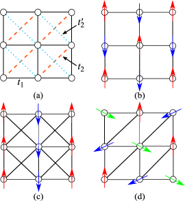
Figure 1: (Color online) (a) Schematic representation of the square-lattice Hubbard model with the isotropic nearest-neighbor hopping parameter $t_{1}$ and anisotropic next-nearest-neighbor parameters $t_{2}$ and $t^{\prime}_{2}$. (b) Isotropic square lattice at $t_{2}=t^{\prime}_{2}=0$. (c) Crossed square lattice at $t_{2}=t^{\prime}_{2}=t_{1}$. (d) Isotropic triangular lattice at $t_{1}=t_{2}$ and $t^{\prime}_{2}=0$. The arrows represent the directions of the electron spins. The sublattices are indicated by different colors.

2 Model and Method

We consider the frustrated Hubbard model defined on the two-dimensional square lattice at half filling as illustrated in Fig. 1. The Hamiltonian is given by

$$H=-t_{1}\sum_{\langle i,j\rangle}\sum_{\sigma}c^{\dagger}_{i\sigma}c_{j\sigma}-t_{2}\sum_{\langle\langle i,j\rangle\rangle}\sum_{\sigma}c^{\dagger}_{i\sigma}c_{j\sigma}$$

$$-t^{\prime}_{2}\sum_{\langle\langle i,j\rangle\rangle^{\prime}}\sum_{\sigma}c^{\dagger}_{i\sigma}c_{j\sigma}+U\sum_{i}n_{i\uparrow}n_{i\downarrow}-\mu\sum_{i,\sigma}n_{i\sigma},$$ (1)

where $c^{\dagger}_{i\sigma}$ is the creation operator of an electron with spin $\sigma$ at site $i$ and $n_{i\sigma}=c^{\dagger}_{i\sigma}c_{i\sigma}$. $\langle i,j\rangle$ indicates the nearest-neighbor bonds with an isotropic hopping parameter $t_{1}$, and $\langle\langle i,j\rangle\rangle$ and $\langle\langle i,j\rangle\rangle^{\prime}$ indicate the next-nearest-neighbor bonds with anisotropic hopping parameters $t_{2}$ and $t^{\prime}_{2}$, respectively [see Fig. 1(a)]. $U$ is the on-site Coulomb repulsion between electrons and $\mu$ is the chemical potential maintaining the system at half filling. In the large-$U$ limit, the model can be mapped onto the frustrated spin-1/2 Heisenberg model

$$H=J_{1}\sum_{\langle i,j\rangle}\bm{S}_{i}\cdot\bm{S}_{j}+J_{2}\sum_{\langle\langle i,j\rangle\rangle}\bm{S}_{i}\cdot\bm{S}_{j}+J^{\prime}_{2}\sum_{\langle\langle i,j\rangle\rangle^{\prime}}\bm{S}_{i}\cdot\bm{S}_{j}$$ (2)

in the second-order perturbation of the hopping parameters with $\bm{S}_{i}=\sum_{\alpha,\beta}c^{\dagger}_{i\alpha}\bm{\sigma}_{\alpha\beta}c_{i\beta}$/2, where $\bm{\sigma}_{\alpha\beta}$ is the vector of Pauli matrices. The exchange coupling constants are given by $J_{1}=4t^{2}_{1}/U$, $J_{2}=4t^{2}_{2}/U$, and $J^{\prime}_{2}=4t^{\prime 2}_{2}/U$ for the lattice shown in Fig. 1(a). We will compare our results of the Hubbard model in the strong correlation regime with those of the frustrated Heisenberg model, for which related studies have been carried out.

We treat a wide parameter space of $0\leq t_{2}/t_{1}\leq 1$ and $0\leq t^{\prime}_{2}/t_{1}\leq 1$, including three limiting cases: (i) at $t_{2}=t^{\prime}_{2}=0$ [square lattice, see Fig. 1(b)], where the Néel order is realized, (ii) at $t_{2}=t^{\prime}_{2}=t_{1}$ [crossed square lattice, see Fig. 1(c)], where the collinear order is realized, and (iii) at $t_{2}=t_{1}$ and $t^{\prime}_{2}=0$ [triangular lattice, see Fig. 1(d)], where the 120^∘ spiral order is realized. We will calculate how the above three ordered phases change when the hopping parameters are varied in the ranges $0\leq t_{2}\leq t_{1}$ and $0\leq t^{\prime}_{2}\leq t_{1}$.

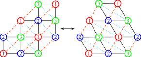
Figure 2: (Color online) Left: twelve-site square-lattice cluster used as a reference system in our analysis. Right: equivalent triangular-lattice cluster, where the three sites 1, 2, and 3 form an equilateral triangle. The anisotropic triangular lattice is defined as $t^{\prime}_{2}=0$ and $t_{1}\neq t_{2}$.

We employ the VCA, which is a quantum cluster method based on SFT [62, 63, 64], where the grand potential $\Omega$ of the original system is given by a functional of the self-energy. By restricting the trial self-energy to that of the reference system $\Sigma^{\prime}$, we obtain the grand potential in the thermodynamic limit as

$$\Omega[\Sigma^{\prime}]=\Omega^{\prime}+\mathrm{Trln}(G_{0}^{-1}-\Sigma^{\prime})^{-1}-\mathrm{Trln}G^{\prime},$$ (3)

where $\Omega^{\prime}$ and $G^{\prime}$ are the exact grand potential and Green function of the reference system, respectively, and $G_{0}$ is the noninteracting Green function. The short-range electron correlations within the cluster of the reference system are taken into account exactly.

The advantage of the VCA is that the spontaneous symmetry breaking can be treated within the framework of the theory. Here, we introduce the Weiss fields for magnetic orderings as variational parameters. The Hamiltonian of the reference system is then given by $H^{\prime}=H+H_{\rm{N}}+H_{\rm{C}}+H_{\rm{S}}$ with

$$H_{\mathrm{N}}=h^{\prime}_{\mathrm{N}}\sum_{i}e^{i\bm{Q}_{\mathrm{N}}\cdot\bm{r}_{i}}S^{z}_{i}$$ (4)

$$H_{\mathrm{C}}=h^{\prime}_{\mathrm{C}}\sum_{i}e^{i\bm{Q}_{\mathrm{C}}\cdot\bm{r}_{i}}S^{z}_{i}$$ (5)

$$H_{\mathrm{S}}=h^{\prime}_{\mathrm{S}}\sum_{i}\bm{e}_{a_{i}}\cdot\bm{S}_{i},$$ (6)

where $h^{\prime}_{\mathrm{N}}$, $h^{\prime}_{\mathrm{C}}$, and $h^{\prime}_{\mathrm{S}}$ are the strengths of the Weiss fields for the Néel, collinear, and spiral orders, respectively. The wave vectors are defined as $\bm{Q}_{\rm{N}}=(\pi,\pi)$ for the Néel order and $\bm{Q}_{\rm{C}}=(\pi,0)$ or $(0,\pi)$ for the collinear order. For the spiral order, the unit vectors $\bm{e}_{a_{i}}$ are rotated by 120^∘ to each other, where $a_{i}$ $(=1,2,3)$ is the sublattice index of site $i$. The variational parameter is optimized on the basis of the variational principle $\partial\Omega/\partial h^{\prime}=0$ for each magnetic order. The solution with $h^{\prime}\neq 0$ corresponds to the ordered state.

We use the twelve-site cluster shown in Fig. 2 as the reference system. This cluster is convenient because we can treat the two-sublattice states (Néel and collinear states) with an equal number of up and down spins and, at the same time, the three-sublattice state (spiral state) with an equal number of three sublattice sites. Note that longer-period phases such as a spiral phase mentioned in a different system [54] and incommensurate ordered phases are difficult to treat in the present approach.

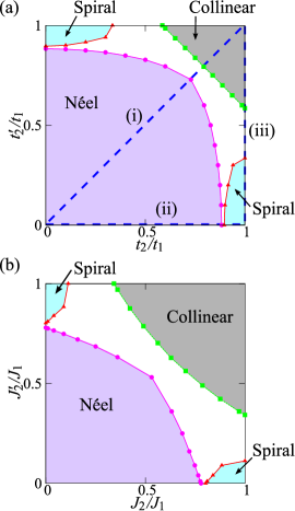
Figure 3: (Color online) (a) Calculated ground-state phase diagram of our model at $U/t_{1}=60$ in the $(t_{2}/t_{1},t^{\prime}_{2}/t_{1})$ plane and (b) converted phase diagram in the $(J_{2}/J_{1},J^{\prime}_{2}/J_{1})$ plane. The uncolored region corresponds to the nonmagnetic insulating phase. The transition to the collinear phase is of the first order (or discontinuous) and the transitions to the Néel and spiral phases are of the second order (or continuous). The phases along dashed lines (i), (ii), and (iii) shown in (a) are circumstantiated in Fig. 4.

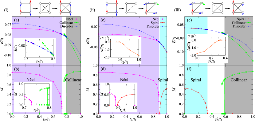
Figure 4: (Color online) Calculated ground-state energies (upper panels) and order parameters (lower panels) for the Néel, collinear, spiral, and nonmagnetic insulating phases as a function of $t_{2}/t_{1}$ or $t^{\prime}_{2}/t_{1}$. The left, middle, and right panels correspond to lines (i), (ii), and (iii) in Fig. 3(a), where we assume $t_{2}=t^{\prime}_{2}$, $t^{\prime}_{2}=0$, and $t_{2}=t_{1}$, respectively. The inset in (c) and (e) displays the energy difference between the spiral and nonmagnetic insulating phases $\Delta E$, and other insets enlarge the region near the phase boundary.

3 Results of Calculations

3.1 Strong correlation regime

First, let us discuss the phase diagram of our model in the strong correlation regime $U/t_{1}=60$. The result is shown in Fig. 3, where the result for our Hubbard model in the $(t_{2}/t_{1},t^{\prime}_{2}/t_{1})$ plane as well as the same result converted to the Heisenberg model parameters $(J_{2}/J_{1},J^{\prime}_{2}/J_{1})$ are shown. We find three ordered phases: the Néel ordered phase around $(t_{2}/t_{1},t^{\prime}_{2}/t_{1})=(0,0)$, the collinear ordered phase around $(t_{2}/t_{1},t^{\prime}_{2}/t_{1})=(1,1)$, and the spiral ordered phase around $(t_{2}/t_{1},t^{\prime}_{2}/t_{1})=(1,0)$ and $(0,1)$. The nonmagnetic insulating phase, which is absent in the classical Heisenberg model (see Appendix A), appears in an intermediate region between the three ordered phases. Thus, the quantum fluctuations in the frustrated spin degrees of freedom are essential in the emergence of the nonmagnetic insulating phase. As shown below, the phase transition to the collinear phase is of the first order (or discontinuous) and the phase transitions to the Néel and spiral phases are of the second order (or continuous). This phase diagram is determined on the basis of the calculated ground-state energies $E=\Omega+\mu$ (per site) and magnetic order parameters $M$ (per site) defined as $M_{\rm{N}}=(2/L)\sum_{i}e^{i\bm{Q}_{\mathrm{N}}\cdot\bm{r}_{i}}\langle S^{z}_{i}\rangle$ for the Néel order, $M_{\rm{C}}=(2/L)\sum_{i}e^{i\bm{Q}_{\mathrm{C}}\cdot\bm{r}_{i}}\langle S^{z}_{i}\rangle$ for the collinear order, and $M_{\rm{S}}=(2/L)\sum_{i}\bm{e}_{a_{i}}\cdot\langle\bm{S}_{i}\rangle$ for the spiral order, where $\langle~{}\rangle$ stands for the ground-state expectation value and $L$ is the number of sites in the system. In the following, we will circumstantiate the obtained phases, particularly along lines (i), (ii), and (iii) drawn in Fig. 3(a), whereby we will discuss some details of our calculated results in comparison with other studies.

Along line (i): The results are shown in the left panels of Fig. 4, where we assume $t_{2}=t^{\prime}_{2}$. At $t_{2}=0$, the ground state is the Néel order, and with increasing $t_{2}$, the energy of the Néel order gradually approaches the energy of the nonmagnetic state. At $t_{2}/t_{1}=0.73$, the energy of the Néel order continuously reaches the energy of the nonmagnetic state and the Néel order disappears. The calculated order parameter indicates a continuous phase transition. At $t_{2}/t_{1}=1$, on the other hand, the ground state is the collinear order. The ground-state energy of the collinear order increases with decreasing $t_{2}$, and at $t_{2}/t_{1}=0.79$, it crosses to the nonmagnetic state, resulting in a discontinuous phase transition, as indicated by the calculated order parameter. The nonmagnetic insulating state thus appears at $0.73<t_{2}/t_{1}<0.79$, which corresponds to the region $0.53<J_{2}/J_{1}<0.63$ in the Heisenberg model parameters. In comparison with previous studies on the $J_{1}$-$J_{2}$ square-lattice Heisenberg model, which have estimated the transition point between the Néel and nonmagnetic phases to be at $J_{2}/J_{1}=0.40-0.44$ [17, 22, 24, 31, 32], our result slightly overestimates the stability of the Néel order. This overestimation may be caused by the cluster geometry used in our calculations; if we use the $2\times 2$ site cluster as the reference system, the transition occurs at $J_{2}/J_{1}=0.42$ [36], which is in good agreement with the previous studies. The transition point between the collinear and nonmagnetic phases, on the other hand, has been estimated to be at $J_{2}/J_{1}=0.59-0.62$ [17, 22, 24, 32], which is in good agreement with our result.

Along line (ii): The results are shown in the middle panels of Fig. 4, where we assume $t^{\prime}_{2}=0$. With increasing $t_{2}$ from $t_{2}=0$, at which the ground state is the Néel order, the energy of the Néel order gradually approaches the energy of the nonmagnetic state, and at $t_{2}/t_{1}=0.88$, the Néel order disappears continuously. The calculated order parameter indicates the continuous phase transition. At $t_{2}/t_{1}=1$, on the other hand, the ground state is the spiral order, although the energy difference between the spiral and nonmagnetic states is very small [see the inset of Fig. 4(c)] due to the strong geometrical frustration of the triangular lattice. With decreasing $t_{2}$ from $t_{2}/t_{1}=1$, the ground-state energy of the spiral order increases gradually and approaches the energy of the nonmagnetic state, and at $t_{2}/t_{1}=0.89$, the spiral order disappears continuously, in agreement with the calculated order parameter. Thus, the nonmagnetic phase appears in a very narrow region of $0.88<t_{2}/t_{1}<0.89$. The corresponding Heisenberg model parameters at which the Néel and spiral orders disappear are around $J_{2}/J_{1}=0.79$. The previous studies for the anisotropic triangular-lattice Heisenberg model [42, 44] have given values around $J_{2}/J_{1}=0.80-0.87$ for the transition point, which are in good agreement with our result.

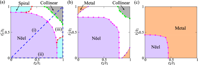
Figure 5: (Color online) Calculated ground-state phase diagrams of our model in the $(t_{2}/t_{1},t^{\prime}_{2}/t_{1})$ plane at (a) $U/t_{1}=10$, (b) $U/t_{1}=6$, and (c) $U/t_{1}=2$. The uncolored regions in (a) and (b) correspond to the nonmagnetic insulating phase. The phases along dashed lines (i), (ii), and (iii) shown in (a) are circumstantiated in Fig. 6.

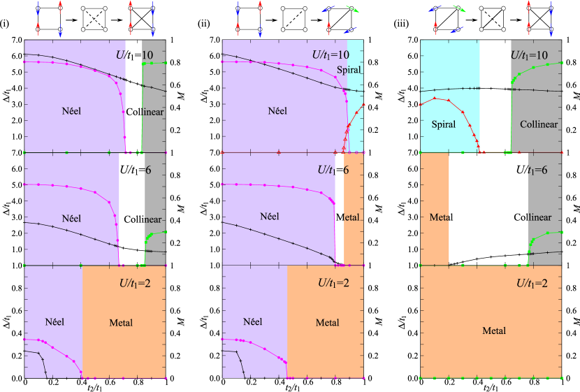
Figure 6: (Color online) Calculated results for the order parameters $M$ (pink, green, and red dots) of the Néel, collinear, and spiral phases and the single-particle gap $\Delta/t_{1}$ (black crosses) at $U/t_{1}=10$ (upper panels), $U/t_{1}=6$ (middle panels), and $U/t_{1}=2$ (lower panels). The left, middle, and right panels correspond to the lines (i), (ii), and (iii) defined in Fig. 5(a), where we assume $t_{2}=t^{\prime}_{2}$, $t^{\prime}_{2}=0$, and $t_{2}=t_{1}$, respectively.

Along line (iii): The results are shown in the right panels of Fig. 4, where we assume $t_{2}=t_{1}$. At $t^{\prime}_{2}=0$, the ground state is the spiral order, although the energy difference from the nonmagnetic state is very small [see the inset of Fig. 4(e)]. With increasing $t^{\prime}_{2}$, the energy of the spiral order gradually approaches the energy of the nonmagnetic state, and at $t^{\prime}_{2}/t_{1}=0.34$, the spiral order disappears continuously, in agreement with the calculated order parameter. On the other hand, with decreasing $t^{\prime}_{2}$ from $t^{\prime}_{2}/t_{1}=1$, at which the collinear order is stable, the ground-state energy of the collinear order increases and crosses to the nonmagnetic state at $t^{\prime}_{2}/t_{1}=0.59$. The transition is thus discontinuous, in agreement with the calculated order parameter. The nonmagnetic state therefore appears at $0.34<t^{\prime}_{2}/t_{1}<0.59$, which corresponds to the region $0.11<J^{\prime}_{2}/J_{1}<0.34$ if we use the Heisenberg model parameters. To our knowledge, no comparable calculations have been made for the frustrated Heisenberg model in this parameter region.

3.2 Intermediate to weak correlation regime

Next, let us discuss the phase diagram of our model in the intermediate to weak correlation regime. The results at $U/t_{1}=10$, $6$, and $2$ are shown in Fig. 5. The detailed results for the calculated single-particle gap and order parameters are also shown in Fig. 6 along lines (i), (ii), and (iii) defined above.

At $U/t_{1}=10$, we find that the results are qualitatively similar to those at $U/t_{1}=60$, except for the transition between the Néel and spiral orders: the nonmagnetic insulating phase appears between these orders at $U/t_{1}=60$ but a direct first-order transition occurs at $U/t_{1}=10$ [55, 56] with a double minimum structure in the grand potential. The nonmagnetic insulating phase appears at $0.71<t_{2}/t_{1}<0.84$ along line (i), which is in good agreement with the previous studies [34, 36], where the values $t_{2}/t_{1}=0.70-0.77$ for the transition between the Néel and nonmagnetic phases and $t_{2}/t_{1}=0.82-0.85$ for the transition between the collinear and nonmagnetic phases were reported. The nonmagnetic phase also appears at $0.42<t^{\prime}_{2}/t_{1}<0.64$ along line (iii).

At $U/t_{1}=6$, we find that the spiral phase disappears and a paramagnetic metallic phase appears in the triangular lattice geometry at $(t_{2}/t_{1},t_{2}^{\prime}/t_{1})\simeq(1,0)$ or $(0,1)$. The nonmagnetic insulating phase appears at $0.66<t_{2}/t_{1}<0.86$ along line (i), the region of which becomes wider with decreasing value of $U/t_{1}$ from 60 to 10 and 6, which is again in good agreement with the previous studies [33, 34]. The region of the nonmagnetic insulating phase also becomes wider along line (iii), which occurs between the collinear and paramagnetic metallic phases. Along line (ii), the nonmagnetic insulating phase with a small charge gap appears again, which is between the Néel and paramagnetic metallic phases [55, 56].

At $U/t_{1}=2$, the paramagnetic metallic phase overwhelms the collinear and nonmagnetic insulating phases, retaining only the Néel ordered phase around $t_{2}/t_{1}=t_{2}^{\prime}/t_{1}=0$. Within the Néel phase, the charge gap opens only at $0<t_{2}/t_{1}<0.16$ and the metallic Néel ordered phase appears at $0.16<t_{2}/t_{1}<0.41$ along line (i) and at $0.16<t_{2}/t_{1}<0.47$ along line (ii). The perfect Fermi surface nesting at $t_{2}/t_{1}=t_{2}^{\prime}/t_{1}=0$ and its deformation away from $t_{2}/t_{1}=t_{2}^{\prime}/t_{1}=0$ are responsible for these results [34]. The generalized magnetic susceptibility $\chi_{0}(\bm{q})$ calculated in the noninteracting limit of our model [Eq. (1)] explains this result (see Appendix B). The transition between the Néel ordered metallic phase and the paramagnetic metallic phase is continuous along line (i) and discontinuous along line (ii).

4 Summary

We have used the VCA based on SFT to study the two-dimensional frustrated Hubbard model at half filling with the isotropic nearest-neighbor and anisotropic next-nearest-neighbor hopping parameters. We have particularly focused on the effect of geometrical frustration on the spin degrees of freedom of the model in a wide parameter space including square, crossed-square, and triangular lattices in a wide range of the interaction strength at zero temperature. We have thereby investigated the metal-insulator transition, the magnetic orders, and the emergence of the nonmagnetic insulating phase, although the phases with incommensurate orders or with longer-period orders than the cluster size used have not been taken into account owing to the limitation of the VCA. We have also calculated the ground-state phase diagram of the corresponding classical Heisenberg model as well as the generalized magnetic susceptibility in the noninteracting limit.

We have thus determined the ground-state phase diagram of the model and found that, in the strong correlation regime, magnetic phases with the Néel, collinear, and spiral orders appear in the parameter space, and a nonmagnetic insulating phase, caused by the effect of quantum fluctuations in the frustrated spin degrees of freedom, emerges in the wide parameter region between these three ordered phases. We have also found that the phase transition from the Néel and spiral orders to the nonmagnetic phase is continuous (or a second-order transition), whereas the transition from the collinear order to the nonmagnetic phase is discontinuous (or a first-order transition). We have compared our results with the results of the corresponding Heisenberg model calculations that have been made so far and found that the agreement is good whenever the comparison is possible. We have also found that, in the intermediate correlation regime, the paramagnetic metallic phase begins to appear in the triangular lattice geometry, which overwhelms the collinear and nonmagnetic insulating phases in the weak correlation regime, retaining only the Néel ordered phase in the square lattice geometry. We hope that our results for the phase diagram obtained in the wide parameter space will encourage future studies on the characterization of the nonmagnetic insulating phase as well as on its experimental relevance.

We thank S. Miyakoshi for useful discussions. T. K. acknowledges support from a JSPS Research Fellowship for Young Scientists. This work was supported in part by a Grant-in-Aid for Scientific Research (No. 26400349) from JSPS of Japan.

Appendix A Ground-State Phase Diagram of the Classical Heisenberg Model

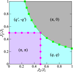
Figure 7: (Color online) Calculated ground-state phase diagram of the corresponding classical Heisenberg model.

Here, we present the ground-state phase diagram of the classical Heisenberg model, which is defined as in Eq. (2) but its quantum spins $\bm{S}_{i}$ are replaced by the classical vectors $\tilde{\bm{S}}$, so that quantum fluctuations of the system are completely suppressed although the frustrative features in the spin degrees of freedom are present. The Hamiltonian is given by $H=\sum_{\bm{q}}J(\bm{q})\,\tilde{\bm{S}}_{-\bm{q}}\cdot\tilde{\bm{S}}_{\bm{q}}$ in momentum space, where

$$J(\bm{q}) =J_{1}(\cos q_{x}+\cos q_{y})+J_{2}\cos(q_{x}+q_{y})$$

$$+J^{\prime}_{2}\cos(q_{x}-q_{y}).$$ (7)

The ground states of the system are calculated [65] and the phase diagram is obtained as shown in Fig. 7. We find that the magnetically ordered ground states appear in the entire parameter space examined, which include the Néel order [$\bm{q}=(\pi,\pi)$], collinear order [$\bm{q}=(\pi,0)$], and spiral orders [$\bm{q}=(q,q)$ and $(q^{\prime},-q^{\prime})$ with $q=\cos^{-1}(-J_{1}/2J_{2})$ and $q^{\prime}=\cos^{-1}(-J_{1}/2J^{\prime}_{2})$]. Therefore, comparing with the results given in the main text, we may conclude that the quantum fluctuations in the geometrically frustrated spin degrees of freedom are essential in the emergence of the nonmagnetic insulating phase discussed in the main text.

Appendix B Generalized Susceptibility in the Noninteracting Limit

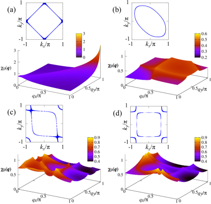
Figure 8: (Color online) Calculated generalized magnetic susceptibility defined in Eq. (8) at (a) $t_{2}/t_{1}=t^{\prime}_{2}/t_{1}=0.0$, (b) $t_{2}/t_{1}=1.0$, $t^{\prime}_{2}/t_{1}=0.0$, (c) $t_{2}/t_{1}=1.0$, $t^{\prime}_{2}/t_{1}=0.8$, and (d) $t_{2}/t_{1}=t^{\prime}_{2}/t_{1}=1.0$. The corresponding Fermi surface is shown in each panel.

Here, we present the generalized magnetic susceptibility (or Lindhard function) at zero frequency [66, 67, 68],

$$\chi_{0}(\bm{q})=\frac{1}{L}\sum_{\bm{k}}\frac{f(\epsilon_{\bm{k}})-f(\epsilon_{\bm{k}+\bm{q}})}{\epsilon_{\bm{k}+\bm{q}}-\epsilon_{\bm{k}}},$$ (8)

calculated for our model [Eq. (1)] in the noninteracting limit, where $\epsilon_{\bm{k}}$ is the corresponding noninteracting band disperson and $f(\epsilon)$ is the Fermi function. The calculated results at temperature $0.01t_{1}$ are shown in Fig. 8, where we find that a diverging behavior appears only at $\bm{q}=(\pi,\pi)$ in Fig. 8(a) due to perfect Fermi surface nesting, which yields the Néel ordered state at $t_{2}/t_{1}=t^{\prime}_{2}/t_{1}=0.0$ in the presence of a small but finite interaction strength $U$. There are characteristic features of $\chi_{0}(\bm{q})$ but no other diverging behaviors are found, indicating the absence of other magnetic orderings in the weak correlation limit.

References

- [1] L. Balents, Nature (London) 464, 199 (2010).
- [2] P. A. Lee, N. Nagaosa, and X.-G. Wen, Rev. Mod. Phys. 78, 17 (2006).
- [3] P. Chandra and B. Doucot, Phys. Rev. B 38, 9335(R) (1988).
- [4] S. Sachdev and R. N. Bhatt, Phys. Rev. B 41, 9323 (1990).
- [5] M. J. de Oliveira, Phys. Rev. B 43, 6181 (1991).
- [6] A. V. Chubukov and T. Jolicoeur, Phys. Rev. B 44, 12050(R) (1991).
- [7] J. Oitmaa and Z. Weihong, Phys. Rev. B 54, 3022 (1996).
- [8] M. E. Zhitomirsky and K. Ueda, Phys. Rev. B 54, 9007 (1996).
- [9] A. E. Trumper, L. O. Manuel, C. J. Gazza, and H. A. Ceccatto, Phys. Rev. Lett. 78, 2216 (1997).
- [10] R. R. P. Singh, Z. Weihong, C. J. Hamer, and J. Oitmaa, Phys. Rev. B 60, 7278 (1999).
- [11] L. Capriotti and S. Sorella, Phys. Rev. Lett. 84, 3173 (2000).
- [12] L. Capriotti, F. Becca, A. Parola, and S. Sorella, Phys. Rev. Lett. 87, 097201 (2001).
- [13] G. M. Zhang, H. Hu, and L. Yu, Phys. Rev. Lett. 91, 067201 (2003).
- [14] K. Takano, Y. Kito, Y. Ono, and K. Sano, Phys. Rev. Lett. 91, 197202 (2003).
- [15] J. Sirker, Z. Weihong, O. P. Sushkov, and J. Oitmaa, Phys. Rev. B 73, 144422 (2006).
- [16] M. Mambrini, A. Läuchli, D. Poilblanc, and F. Mila, Phys. Rev. B 74, 144422 (2006).
- [17] R. Darradi, O. Derzhko, R. Zinke, J. Schulenburg, S. E. Krüger, and J. Richter, Phys. Rev. B 78, 214415 (2008).
- [18] L. Isaev, G. Ortiz, and J. Dukelsky, Phys. Rev. B 79, 024409 (2009).
- [19] K. S. D. Beach, Phys. Rev. B 79, 224431 (2009).
- [20] J. Ritcher and J. Schulenburg, Eur. Phys. J. B 73, 117 (2010).
- [21] J. Reuther and P. Wölfle, Phys. Rev. B 81, 144410 (2010).
- [22] J. F. Yu and Y. J. Kao, Phys. Rev. B 85, 094407 (2012).
- [23] L. Wang, Z. C. Gu, F. Verstraete, and X. G. Wen, arXiv:1112.3331.
- [24] H.-C. Jiang, H. Yao, and L. Balents, Phys. Rev. B 86, 024424 (2012).
- [25] F. Mezzacapo, Phys. Rev. B 86, 045115 (2012).
- [26] T. Li, F. Becca, W. J. Hu, and S. Sorella, Phys. Rev. B 86, 075111 (2012).
- [27] L. Wang, D. Poilblanc, Z. C. Gu, X. G. Wen, and F. Verstraete, Phys. Rev. Lett. 111, 037202 (2013).
- [28] W. J. Hu, F. Becca, A. Parola, and S. Sorella, Phys. Rev. B 88, 060402 (2013).
- [29] R. L. Doretto, Phys. Rev. B 89, 104415 (2014).
- [30] Y. Qi and Z. C. Gu, Phys. Rev. B 89, 235122 (2014).
- [31] S.-S. Gong, W. Zhu, D. N. Sheng, O. I. Motrunich, and M. P. A. Fisher, Phys. Rev. Lett. 113, 027201 (2014).
- [32] S. Morita, R. Kaneko, and M. Imada, J. Phys. Soc. Jpn. 84, 024720 (2015).
- [33] T. Mizusaki and M. Imada, Phys. Rev. B 74, 014421 (2006).
- [34] A. H. Nevidomskyy, C. Scheiber, D. Sénéchal, and A.-M. S. Tremblay, Phys. Rev. B 77, 064427 (2008).
- [35] Z.-Q. Yu and L. Yin, Phys. Rev. B 81, 195122 (2010).
- [36] S. Yamaki, K. Seki, and Y. Ohta, Phys. Rev. B 87, 125112 (2013).
- [37] P. Sindzingre, P. Lecheminant, and C. Lhuillier, Phys. Rev. B 50, 3108 (1994).
- [38] J. Merino, R. H. McKenzie, J. B. Marston, and C. H. Chung, J. Phys.: Condens. Matter 11, 2965 (1999).
- [39] Z. Weihong, R. H. McKenzie, and R. R. P. Singh, Phys. Rev. B 59, 14367 (1999).
- [40] A. E. Trumper, Phys. Rev. B 60, 2987 (1999).
- [41] S. Yunoki and S. Sorella, Phys. Rev. B 74, 014408 (2006); D. Heidarian, S. Sorella, and F. Becca, Phys. Rev. B 80, 012404 (2009).
- [42] M. Q. Weng, D. N. Sheng, Z. Y. Weng, and R. J. Bursill, Phys. Rev. B 74, 012407 (2006); A. Weichselbaum and S. R. White, Phys. Rev. B 84, 245130 (2011).
- [43] O. A. Starykh and L. Balents, Phys. Rev. Lett. 98, 077205 (2007).
- [44] R. F. Bishop, P. H. Y. Li, D. J. J. Farnell, and C. E. Campbell, Phys. Rev. B 79, 174405 (2009).
- [45] J. Reuther and R. Thomale, Phys. Rev. B 83, 024402 (2011).
- [46] A. Weichselbaum and S. R. White, Phys. Rev. B 84, 245130 (2011).
- [47] P. Hauke, T. Roscilde, V. Murg, J. Cirac, and R. Schmied, New J. Phys. 13, 075017 (2011).
- [48] P. Hauke, Phys. Rev. B 87, 014415 (2013).
- [49] J. Merino, M. Holt, and B. J. Powell, Phys. Rev. B 89, 245112 (2014).
- [50] H. Morita, S. Watanabe, and M. Imada, J. Phys. Soc. Jpn. 71, 2109 (2002).
- [51] P. Sahebsara and D. Seńećhal, Phys. Rev. Lett. 97, 257004 (2006).
- [52] T. Watanabe, H. Yokoyama, Y. Tanaka, and J. Inoue, Phys. Rev. B 77, 214505 (2008).
- [53] L. F. Tocchio, A. Parola, C. Gros, and F. Becca, Phys. Rev. B 80, 064419 (2009).
- [54] L. F. Tocchio, H. Feldner, F. Becca, R. Valenti, and C. Gros, Phys. Rev. B 87, 035143 (2013).
- [55] A. Yamada, Phys. Rev. B 89, 195108 (2014).
- [56] M. Laubach, R. Thomale, C. Platt, W. Hanke, and G. Li, Phys. Rev. B 91, 245125 (2015).
- [57] R. V. Mishmash, J. R. Garrison, S. Bieri, and C. Xu, Phys. Rev. Lett. 111, 157203 (2013).
- [58] R. Kaneko, S. Morita, and M. Imada, J. Phys. Soc. Jpn. 83, 093707 (2014).
- [59] P. H. Y. Li, R. F. Bishop, and C. E. Campbell, Phys. Rev. B 91, 014426 (2015).
- [60] Z. Zhu and S. R. White, Phys. Rev. B 92, 041105(R) (2015).
- [61] W.-J. Hu, S.-S. Gong, W. Zhu, and D. N. Sheng, Phys. Rev. B 92, 140403(R) (2015).
- [62] M. Potthoff, M. Aichhorn, and C. Dahnken, Phys. Rev. Lett. 91, 206402 (2003).
- [63] M. Potthoff, Eur. Phys. J. B 32, 429; 36, 335 (2003).
- [64] C. Dahnken, M. Aichhorn, W. Hanke, E. Arrigoni, and M. Potthoff, Phys. Rev. B 70, 245110 (2004).
- [65] J. M. Luttinger and L. Tisza, Phys. Rev. 70, 954 (1946).
- [66] J. E. Hirsch, Phys. Rev. B 31, 4403 (1985).
- [67] N. Bulut, D. J. Scalapino, and S. R. White, Phys. Rev. B 47, 2742 (1993).
- [68] A. Sherman and M. Schreiber, Phys. Rev. B 76, 245112 (2007).