Quantum Darwinism and non-Markovian dissipative dynamics from quantum phases of the spin$-1/2$ XX model

Abstract

Quantum Darwinism explains the emergence of a classical description of objects in terms of the creation of many redundant registers in an environment containing their classical information. This amplification phenomenon, where only classical information reaches the macroscopic observer and through which different observers can agree on the objective existence of such object, has been revived lately for several types of situations, successfully explaining classicality. We explore quantum Darwinism in the setting of an environment made of two level systems which are initially prepared in the ground state of the XX model, which exhibits different phases; we find that the different phases have different ability to redundantly acquire classical information about the system, being the “ferromagnetic phase” the only one able to complete quantum Darwinism. At the same time we relate this ability to how non-Markovian the system dynamics is, based on the interpretation that non-Markovian dynamics is associated to back flow of information from environment to system, thus spoiling the information transfer needed for Darwinism. Finally, we explore mixing of bath registers by allowing a small interaction among them, finding that this spoils the stored information as previously found in the literature.

I Introduction

Quantum Darwinism deals with the description and the quantification of the reasons why quasi-classical states play a special role in our world, as they are perfectly suitable to describe what happens in a broad range of scales zurekNAT . Indeed, in our daily experience, we only observe phenomena that can be described by classical laws, despite the fact that classical states represent a very tiny fraction of the whole Hilbert space of the Universe.

The theory of open quantum systems explains the emergence of classicality as the result of the interaction of a small system with a larger one representing the environment. Decoherence is the tool used to describe the transition from quantum to classical states through the loss of information from the system towards the environment deco1 ; deco2 . When describing the emergence of decoherence, a partial trace is performed over the bath’s degrees of freedom, that is, the information contained in the environment is not accessible at all. Because of the decoherence process, there are states that naturally emerge due to their stability with respect to the interaction with the bath. These states, usually referred to as pointer states pointer , are the best candidates to describe the classical world.

In addition, most of the information we have about any system comes from indirect observations made on fragments of the environment rather than on the system itself. The fact that different observers accessing different fragments get the same information about the system is the central result of quantum Darwinism: the states perceived in the same way (objectively) by multiples observers are the ones that are able to spread around them multiple copies of their classical information content. This illustrates the emergence of an objective classical reality from the quantum probabilistic world.

Recently it has been shown brandao that observers monitoring a system by measuring its environment can only learn about a unique (pointer) observable, this being a generic feature of quantum mechanics. However this is only part of the program: observers need to be able to obtain close to full classical information on the system and agree among them. This latter redundant proliferation of information regarding pointer states, far from being generic, has been demonstrated to take place in different physical contexts, that is, considering purely dephasing Hamiltonians zurekCHER , photon environments zurekPHOTON ; korbicz , spin environments spins1 ; haziness ; zurekFALL and Brownian motion brownian1 ; brownian2 ; brownian3 . It has recently been stressed that this redundant encoding should be checked at the level of states, with a spectrum broadcast structure origin .

The achievement of quantum Darwinism, obviously related to which Hamiltonians govern the problem, is also determined by the initial state of the bath. The inhibition of redundancy in Brownian motion has recently been linked galve14 to the presence of non-Markovianity in the open quantum system dynamics nm ; nm2 . Intuitively: the rollback of the decoherence process, through which the environment learns about the system, and which is a salient feature of non-Markovian evolution, is expected to spoil records of the system imprinted upon the environment. In the case of spins, it is known that mixedness and misalignment haziness (the closeness of bath states to eigenstates of the interaction Hamiltonian) of environmental units will reduce the bath’s ability to produce Darwinism. Also, if the bath units are interacting zurekFALL , the redundant classical records will spread and become inaccessible locally, which in the end forces observers to collect huge amounts of bath fragments thus ruining Darwinism.

In this paper we will first consider the role of initial correlations in a separable environment: an ensemble of (uncoupled) spins is prepared in the ground state of the (coupled) XX model in the presence of an external magnetic field. In fact, by tuning the value of the field, different ground states with different correlation properties are available. It will be shown that an initially uncorrelated environment is more liable to produce quantum Darwinism. Second, by gently turning on the XX coupling Hamiltonian among bath spins, we will show that redundant classical records in the bath are spoiled in proportion to the coupling. Finally, we analyze the non-Markovianity of the system’s evolution showing that its behaviour follows the same trend of quantum Darwinism. We end our work conjecturing a possible relation between the two phenomena, based on the amount of inter-correlations present in the environment as a pernicious influence.

II Quantum Darwinism

Quantum Darwinism is complete when the environment is able to store redundantly copies of the classical information about a pointer observable of the system, meaning that any other information about the system has not ‘survived’ the (time) evolution. This is typically quantified by the mutual information between the system and fractions ${\mathcal{F}}$ of the environment: classical, objective existence of the system needs different observers, who can access different and independent fractions of the environment, to agree on the properties of the system by querying such fractions. The size of the fractions should not be a limitation, since otherwise we would need a minimum amount of environment to learn something about the system. Mathematically this condition basically means that the mutual information between system and fractions of the environment $I(S:{\mathcal{F}})$ must be almost independent of fraction size ($\#\mathcal{F}$) and on which fraction we have chosen (i.e. $I(S:\mathcal{F})\neq f(\#\mathcal{F})$ and $I(S:{\mathcal{F}}_{1})=I(S:{\mathcal{F}}_{2})$ when $\#\mathcal{F}_{1}=\#\mathcal{F}_{2}$).

Let us consider a system $S$ in contact with an environment ${\cal E}$ and suppose that we have knowledge about the inner structure of ${\cal E}$, that is ${\cal E}=\otimes_{i=1}^{N}{\cal E}_{i}$, where each ${\cal E}_{i}$ has dimension $D$. We also suppose that any individual fragment of the environment ${\cal F}=\otimes_{i=1}^{\#\mathcal{F}}{\cal E}_{i}$ of size $\#\mathcal{F}=fN$ ($f\cdot N$, with $0\leq f\leq 1$, is the number of ${\cal E}$ ’s spins contained in ${\cal F}$) is accessible. The mutual information between $S$ and ${\cal F}$, which quantifies how much information about $S$ is present in the fragment ${\cal F}$ is defined as

$${\cal I}(S:{\mathcal{F}})=H_{S}+H_{{\cal F}}-H_{S{\cal F}},$$ (1)

where $H$ is the von Neumann entropy. The emergence of Darwinism can be explained by the following example: the pure system+environment state

$$|\phi_{SE}\rangle=(\alpha|0\rangle+\beta|1\rangle)\otimes|\varepsilon^{(0)},\varepsilon^{(1)},\dots,\varepsilon^{(N)}\rangle$$ (2)

evolves into

$$|\phi_{SE}^{\prime}\rangle=\alpha|0\rangle|\varepsilon_{0}^{(0)},\varepsilon_{0}^{(1)},\dots,\varepsilon_{0}^{(N)}\rangle+\beta|1\rangle|\varepsilon_{1}^{(0)},\varepsilon_{1}^{(1)},\dots,\varepsilon_{1}^{(N)}\rangle,$$ (3)

where $\langle\varepsilon_{i}^{(n)}|\varepsilon_{j}^{(m)}\rangle=\delta_{ij}$. In such a GHZ state, the information carried out by the system can be also found considering any possible environment fraction of any size. In fact, all the reduced density matrices have the same entropy and, for any $\#\mathcal{F}$ excluding $0$ and $N$, $I(S:{\mathcal{F}})=H_{S}$, where $\rho_{S}$ is the density matrix of the system after the bath has been traced out. If the total state $S+{\cal E}$ is pure, measuring the whole environment, one acquires full knowledge about the state of the system, given that $H_{S}=H_{{\cal E}}$. As a further example, let us consider a random pure state. Is it possible to get a high amount of information monitoring only a small part of the bath? What happens is that, typically, the observer cannot learn anything about a system without sampling at least half of its environment. This characteristic behavior is illustrated in Refs.zurekabstract1 ; zurekabstract2 . In turn, states created by decoherence, which do not follow this behavior and are those explaining our everyday classical experience, have zero measure in the thermodynamic limit.

It is pretty natural to ask whether the presence of correlations in the environment facilitates the emergence of quantum Darwinism. Here, we address this problem considering the following model: a single spin $S$ (the system) couples to a collection of $N$ spins, decoupled from each other. The Hamiltonian considered is $H=H_{S}+H_{B}+H_{S\cal E}$, where

$$H_{B} = -\sum_{i=1}^{N}(\sigma_{i}^{+}\sigma_{i+1}^{-}+\sigma_{i}^{-}\sigma_{i+1}^{+})-h\sum_{i=1}^{N}\sigma_{i}^{z},$$ (4)

$$H_{S\cal E} = d\;\sigma_{S}^{z}\otimes\sum_{i=1}^{N}\sigma_{i}^{x}.$$ (5)

Here, $N$ is the total number of spins in the bath, $h$ is the strength of the external magnetic field, and periodic boundary conditions are imposed. Assuming $[H_{S},H_{S\cal E}]=0$, the system timescales are of no importance and will be neglected, that is, we will neglect $H_{S}$ unless otherwise specified.

Usually, open quantum systems are studied in the weak-coupling regime. However, as we have said in the introduction, we want to investigate the ability of this spin bath to store classical copies of the system. Then, the bath itself must be modified during the dynamics. To this end, we will consider a system-bath interaction much higher than the bath Hamiltonian itself ($d\gg h\sim 1$), whose effects on the dynamics can be neglected at least as a first approximation.

The initial state of the system is $|+\rangle=(|\uparrow\rangle+|\downarrow\rangle)/\sqrt{2}$, while, assuming zero temperature, the bath is initially prepared in its ground state $|G\rangle$. As $[H_{S},H_{S\cal E}]=0$, the evolution of the global state takes the form

$$|\phi_{SE}(t)\rangle=\frac{1}{\sqrt{2}}(|\uparrow\rangle|G^{\uparrow}\rangle(t)+|\downarrow\rangle|G^{\downarrow}\rangle(t)).$$ (6)

The system undergoes pure dephasing, that is, its density matrix evolves in time as

$$\rho_{S}(t)=\frac{1}{2}\left(\begin{array}[]{cc}1&\nu(t)\\ \nu^{*}(t)&1\end{array}\right),$$ (7)

where $\nu(t)=\langle G^{\downarrow}|G^{\uparrow}\rangle$.

As we are going to prove, different forms for the ground state show different capability of storing redundant copies of classical information of the system.

III Quantum phases

In this section we briefly review some of the properties of the isotropic $XX$ Hamiltonian in the presence of a transverse field, which is exactly the model introduced in (4) to describe the bath.

The exact spectrum of $H_{B}$ can be calculated using the Jordan-Wigner transformation, which maps spins into spinless fermions lieb . This model is known not to possess a proper quantum phase transition (QPT). Instead, an infinite-order Kosterlitz-Thouless (KT) kt quantum phase transition without symmetry breaking takes place around $h=h_{C}=1$.

Depending on the value of the transverse field $h$, which plays the role of an effective chemical potential, the number of fermionic excitations in the ground state changes. In the following, $|G_{n}\rangle$ will indicate the ground state in the $n$-excitation sector. Notice that each $|G_{n}\rangle$ is the ground state for a finite range of values of $h$, and that the number of sectors $\bar{n}$ depends on the number of spins in the bath as $\bar{n}=(N/2+1)$ for $N$ even and $\bar{n}=(N+1)/2$ for $N$ odd. For $h\geq h_{C}$, no excitations are present, that is, the ground state is $|G_{0}\rangle$, while $|G_{\bar{n}-1}\rangle$ is the ground state in the region near $h=0$. In the thermodynamic limit, the magnetization grows continuously from $h=0$ up to $h=1$ and then remains constant showing a cusp around $h=h_{C}$ barouch .

IV Results

IV.1 Quantum Darwinism from ground state ordering

As said before, we discuss the emergence of Darwinism preparing the bath in its ground level. At the initial time we assume

$$|\psi(0)\rangle=|+\rangle\otimes|G_{n}\rangle.$$ (8)

In the strong coupling regime, that is, neglecting $H_{B}$ during the dynamics, the evolution is given as

$$|\psi(t)\rangle=e^{-iH_{S\cal E}t}|\psi(0)\rangle.$$ (9)

Because of the form of the interaction, the initial state evolves spanning the whole set of $2^{N+1}$ basis states. Such an exponential dependence strongly limits the maximum number of spins that can be introduced to obtain the numerical solution in computationally reasonable times. However, if the bath’s initial (ground) state is either $|G\rangle=|G_{0}\rangle$ or $|G\rangle=|G_{1}\rangle$, due to the invariance of these states under any spin-spin swap, the effective action of $H_{S\cal E}$ takes a very simple form. Let us indicate with $|\textbf{i}\rangle$ the $i$-magnon state, that is the swap-invariant state with $i$ $1$s and $(N-i)$ $0$s; for instance $|G_{0}\rangle=|\textbf{0}\rangle$ and $|G_{1}\rangle=|\textbf{1}\rangle$. Consider also that

$$e^{-iH_{S\cal E}t}|\psi(0)\rangle = e^{-id\sigma_{S}^{z}\sum_{i}\sigma_{i}^{x}t}|\psi(0)\rangle$$

$$= e^{-id\sum_{i}\sigma_{i}^{x}t}|\uparrow\rangle|G\rangle+e^{+id\sum_{i}\sigma_{i}^{x}t}|\downarrow\rangle|G\rangle.$$

It is easy to show that $\sum_{i}\sigma_{i}^{x}$ couples $|\textbf{i}\rangle$ to $|\textbf{i+1}\rangle$ and to $|\textbf{i-1}\rangle$, with no other states involved.

Then, as detailed in the appendix, an effective Hamiltonian with $N+1$ degrees of freedom can be built to describe evolution (9) of (8) :

$$H_{{\rm eff}}=\sum_{n=0}^{N}(A_{n}^{+}|\textbf{n}\rangle\langle\textbf{n+1}|+A_{n}^{-}|\textbf{n}\rangle\langle\textbf{n-1}|)$$ (10)

where $A_{n}^{-}=\sqrt{n(N-n+1)}$ and $A_{n}^{+}=A_{n+1}^{-}$. As the transition from $|G\rangle=|G_{0}\rangle$ to $|G\rangle=|G_{1}\rangle$ takes place at $h_{C}$, we can monitor the qualitative change around the critical point by considering very long chains.

The simple form of the evolution operator allows us to learn about the recurrence time of the system. In fact, we have

$$|\psi(\pi/2d)\rangle=U_{X}|\psi(0)\rangle,$$ (11)

where $U_{X}=\otimes_{i=1}^{N}\sigma^{x}_{i}$ is the spin flip operator. Then, at $d\cdot t=\pi/2$, the evolved state is identical to the initial one provided that the exchange $|\uparrow\rangle\leftrightarrows|\downarrow\rangle$ has been applied to every single spin. Then, as far as the information content of the state is considered, $\pi/2$ represents the model periodicity, and $\pi/4$ the time when the influence of the environment over the state is maximized before revival takes place. Based on these considerations, we also expect that quantum Darwinism effects are more evident for $\pi/4$.

In Fig. 1, we chose the optimal time $d\cdot t=\pi/4$ and calculated ${\cal I}(S:{\mathcal{F}})$ as a function of $\#\mathcal{F}$ and for different values of $h$ in order to take into account any of the possible ground states $|G_{n}\rangle$ of $H_{B}$ for a bath of $14$ spins. From Fig. 1, we learn that the presence of correlations in the initial state ($h<h_{C}$) has the tendency to destroy the emergence of quantum Darwinism, while as expected, uncorrelated states ($h\geq h_{C}$) bring perfect redundant information proliferation. When moving towards lower values of $h$ (lighter curves) the behavior of ${\cal I}(S:{\mathcal{F}})$ tends to the one observed picking random states (no Darwinism); however for very low $h$ the shape returns to a Darwinism-like one, even though the achieved slope is far from being optimal.

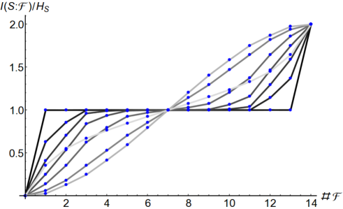
Figure 1: ${\cal I}(S:{\mathcal{F}})$ at $t=\pi/4$ for $N=14$ and in the strong-coupling regime $d=\infty$ for different values of $h$. The eight lines correspond to the eight different ground states of $H_{B}$. The darker the line, the higher the value of $h$. For $h=h_{C}=1$ (black curve) ${\cal I}(S:{\mathcal{F}})=H_{S}$ for any size of the fraction: even observing only one spin in the bath we can learn all the classical information on the system; quantum Darwinism has been fully achieved. For lower $h$ (the lightest line corresponds to the ground state of the sector $0\leq h\lesssim 0.11$) a significant fraction size ($\#{\cal F}\sim N/2$) has to be observed in order to reach enough information (${\cal I}(S:{\mathcal{F}})\sim H_{S}$), so quantum Darwinism has not succeeded.

A possible intuitive explanation of the observed trend, although it will have to remain as a conjecture at this stage, comes from studying the entanglement properties of ground states of the XY model, both bipartite osborne and multipartite giampaolo . When we take a given fraction, its initial entropy is higher when it is more entangled with the rest of the bath, thus more (multipartite) entanglement means more initial entropy of the fraction and thus less ability to store new info about the system. Thus, as discussed in haziness , the best situation for Darwinism is when each bath unit is initially pure (no entropy, so it can grow its entropy maximally through learning the system’s state) and when they are orthogonally aligned to the eigenbasis of the interaction Hamiltonian (this is why the $h=h_{C}$ case is optimal). As we go away from $h=h_{C}$ to lower field values, multipartite entanglement increases each fraction entropy and worsens the ability to produce darwinism. However, when the ground state is half filled, that is, when $h\sim 0$, a new competing effect appears: the system von Neumann entropy drops dramatically close to zero at the time when Darwinism is expected to appear (not shown). At the same time, the bath’s single fraction density matrix remains maximally mixed. Because of this drop, the difference between $H_{{\cal F}}$ and $H_{S{\cal F}}$ becomes less relevant and the Darwinism measure is more sustained (i.e. better) than in the presence of more intense values of the magnetic field. This means that we are facing a non-linear type effect: the multipartite entanglement initially present in the bath is able to induce a small amount of disorder in the system without losing its properties.

IV.2 Mixing of classical records

We have seen that initially correlated states in the bath ($h<h_{C}=1$) perform worse in terms of quantum Darwinism. This means that they are less able to store redundant copies of the classical information about the system. A further aspect, as studied e.g. in zurekFALL , is whether classical redundant copies are stable along time. In that work, the authors study a spin dephasing star model in which they add random weak couplings among bath units; such couplings introduce mixing among the records, thereby leading to a delocalization of the system’s information. It is thus no longer possible to recover such information by just measuring a small, local, fraction of the environment, hence leading to poor Darwinism.

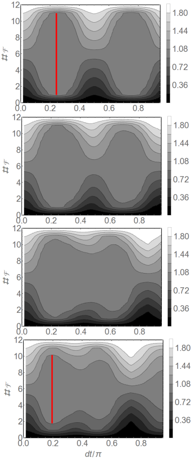
Figure 2: Full evolution of ${\cal I}(S:{\mathcal{F}})$ including the bath’s Hamiltonian, with $d=h=1$, $N=12$ and $H=H_{S\cal E}+\lambda H_{B}$. From top to bottom: $\lambda=0,0.25,0.5,1$. In the $\lambda=0$ case a perfect plateau is seen at $d\cdot t=\pi/4$ (we have drawn a red line to highlight the plateau) and full dynamics recurrence time occurs at $d\cdot t=\pi/2$. Once the bath Hamiltonian comes into play $\lambda\neq 0$, the first plateau gets narrower due to mixing of records in the environment, and even more so the second plateau. Also the recurrence dynamics gets shorter and distorted. The more important is the role of the bath’s Hamiltonian, for higher $\lambda$, the more pronounced is the effect. Mixing of bath records breaks the quantum Darwinism plateau.

Here we have so far studied the case of evolution dictated by only $H_{S\cal E}$, which imprints the information of the system onto the bath. But what happens if the self-dynamics of the bath is taken into account? The Hamiltonian $H_{B}$ consists of a local (field $h$) part and a term (XX interaction) which propagates interaction among bath units, therefore it is to be assumed that $H_{B}$ will mix different local records and diffuse such information in a nonlocal fashion all over the bath’s extension. If so, a worse plateau should be observed. Indeed, in Fig. 2 we see that such is the case. There we let system and bath evolve according to $H=H_{S\cal E}+\lambda H_{B}$ for different values of $\lambda$ (to be compared with results in previous section where we set $d=1$ and $\lambda=0$, which is the equivalent of $d\gg 1$). A progressive worsening of the plateaus for higher $\lambda$s can be observed, in addition to a distortion of the periodicity which was present when only $H_{S\cal E}$ was active.

IV.3 Non-Markovianity

So far, we have studied the emergence of Darwinism induced by the system-bath interaction. As we are working in the strong-coupling regime, it is quite natural to expect that memory effects come out together with a a flux of information from the bath to the system. The connection between non-Markovianity and Darwinism was discussed in Ref. galve14 considering a harmonic oscillator whose position was coupled to the positions of $N$ harmonic oscillators representing the bath. In that context, it was shown that the presence of memory effects inhibits the emergence of objective reality. The same kind of analysis can be carried out considering the model under investigation.

The measure introduced in Ref. nm provides a way of quantifying the amount of non-Markovianity produced during the dynamics. Let us briefly recall such a definition. In a Markovian process, the distinguishability between any pair of quantum states is a monotonously decreasing function of time. Then, the presence of time windows where some states become more distinguishable between each other witnesses the presence of non-Markovianity in the dynamical map. The non-Markovian quantifier is then defined as

$$\mathcal{N}=\max_{\rho_{1},\rho_{2}}\int_{\sigma>0}dt\;\sigma(t,\rho_{1,2}(0)),$$ (12)

where the trace distance, which quantifies distinguishability is $D(\rho_{1},\rho_{2})={\rm Tr}|\rho_{1}-\rho_{2}|/2$ and where its rate of change is $\sigma[t,\rho_{1,2}(0)]=dD[\rho_{1}(t),\rho_{2}(t)]/dt$. The maximum in Eq. (12) is taken over any possible pair of states $\{\rho_{1},\rho_{2}\}$. In the case of pure dephasing, it was shown in Ref. he that there is a simple way of calculating $\mathcal{N}$ in terms of the Loschmidt echo: the trace distance of any pair of (qubit) system states is $D[\rho^{1}_{s}(t),\rho^{2}_{s}(t)]=\sqrt{L(t)}$, where the Loschmidt echo is $L(t)=|\nu(t)|^{2}$.

In Fig. 3 we plot ${\cal N}$ as a function of $h$ for a bath of $12$ spins. The measure is taken considering times between zero and $\pi/4$. In agreement with the results of Ref. galve14 , the evolution is completely Markovian for $h\geq h_{C}$. By lowering the value of $h$ and passing through the whole family of $|G_{n}\rangle$, the value of ${\cal N}$ increases monotonically as magnetization decreases and reaches its maximum for $h=0$. From this point of view, the result is qualitatively similar to the one obtained considering Darwinism. In other words, the higher the amount of non-Markovianity, the smaller the ability of proliferating throughout the environment.

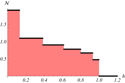
Figure 3: Non-Markovian quantifier $\mathcal{N}$ for a $12$-spin bath in the strong-coupling regime.

A more detailed analysis can be given calculating $\mathcal{N}$ around $h=h_{C}$ by means of the exact solution introduced in Sec. IV.1. As expected, for $h\geq h_{C}$, $\mathcal{N}=0$ irrespective of the bath’s size. More interesting is the behavior immediately below the critical point. Indeed, except for the case of very short chains ($N\lesssim 8$), $\mathcal{N}(h_{C}^{-})$ has a constant value (see Fig. 4). In a way, $\mathcal{N}$ plays the role of a precursor of KT phase transition, as the critical point can be spotted far before reaching the thermodynamic limit by monitoring the amount of non-Markovianity.

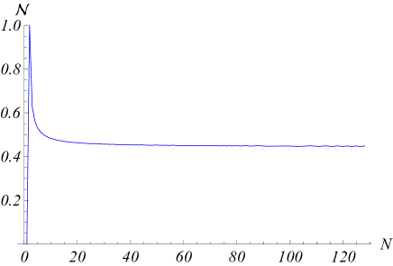
Figure 4: Non-Markovianity immediately before the critical point $\mathcal{N}(h_{C}^{-})$ as a function of the bath size $N$.

V Conclusions

In conclusion, we have studied several aspects of the emergence of quantum Darwinism in the pure-decoherence setting due to a spin bath. We have chosen to initialize the bath in different quantum phases of the isotropic XX model with transverse field. If the initial bath’s state is uncorrelated ($h\geq h_{C}$), as already known, quantum Darwinism arises as redundant proliferation of information is produced throughout the bath. The presence of initial correlations ($h<h_{C}$), however, represents an obstacle towards the building up of classical objectivity.

We have also quantified the amount of non-Markovianity of the system’s dynamics, finding that it correlates well with the absence of quantum Darwinism. This offers further evidence of what was already shown in galve14 for the Brownian oscillator model.

Finally, along the lines presented in zurekFALL , we have shown that coupling between spins in the bath necessarily ruins the achieved redundant classical information storage. This can be understood as mixing and delocalization of such records, whereby information can no longer be gained locally through small bath’s fragments.

As a main conclusion, we have found that the quantum Darwinism program is better achieved if the environment is similar to a blank slate (no correlations) made of uncoupled units, as intuitively is to be expected from any good memory device.

Appendix A Simplified exact solution around the critical point

According to the notation introduced in the main text, for fields immediately smaller than $h_{C}$, the ground state of $H_{B}$ is the single-magnon state

$$|G_{1}\rangle=\frac{1}{\sqrt{N}}\sum_{i}|0,0,\dots,1_{i},\dots,0\rangle.$$ (13)

Let us assume that the bath is initially prepared in $|G\rangle=|G_{0}\rangle$ or in $|G\rangle=|G_{1}\rangle$, while the initial state of the system is $|+\rangle=(|0\rangle+|1\rangle)/\sqrt{2}$. Due to the purely dephasing character of the coupling, the evolution in time $|\psi(t)\rangle=e^{-iHt}|G\rangle\otimes|+\rangle$ can be split into

$$|\psi(t)\rangle=\frac{1}{\sqrt{2}}(e^{-iH_{0}t}|G\rangle\otimes|0\rangle+e^{-iH_{1}t}|G\rangle\otimes|1\rangle)$$ (14)

where $H_{0}=-H_{1}=\sum_{i=1}^{N}\sigma_{i}^{x}$ only involve bath degrees of freedom.

Given that $|G\rangle$ is invariant under any spin-spin swap, its evolution takes a very simple form. Let us indicate with $|\textbf{i}\rangle$ the $i$-magnon state, that is the swap-invariant state with $i$ $1$s (let us point out that $|\textbf{i}\rangle\neq|G_{i}\rangle$ unless $i=0,1$). It is easy to show that $H_{0}$ couples $|\textbf{i}\rangle$ to $|\textbf{i+1}\rangle$ and to $|\textbf{i-1}\rangle$, with no other states involved. Then, an effective Hamiltonian with $N+1$ degrees of freedom can be built to describe the evolution of $|G\rangle$:

$$H_{{\rm eff}}=\sum_{n=0}^{N}(A_{n}^{+}|\textbf{n}\rangle\langle\textbf{n+1}|+A_{n}^{-}|\textbf{n}\rangle\langle\textbf{n-1}|)$$ (15)

where $A_{n}^{-}=\sqrt{n(N-n+1)}$ and $A_{n}^{+}=A_{n+1}^{-}$.

Once the effective Hamiltonian has been derived, the exact dynamics of the initial state $|G\rangle\otimes|+\rangle$ takes the form

$$|\psi(t)\rangle=\frac{1}{\sqrt{2}}\sum_{n=0}^{N}[c_{n}(t)|\textbf{n}\rangle\otimes|0\rangle+c_{n}(-t)|\textbf{n}\rangle\otimes|1\rangle].$$ (16)

The reduced density matrix of the system is then given by

$$\rho_{S}(t)=\frac{1}{2}\left(\begin{array}[]{cc}1&\nu(t)\\ \nu^{*}(t)&1\end{array}\right)$$ (17)

where $\nu(t)=\sum_{n}c_{n}^{2}(t)$.

If we want to calculate the reduced density matrices of fractions of the bath we need to decompose the states n into sub-parts. As all the states involved have long-range correlations, we will limit our calculation to considering the first $k$ spins of the baths (the result would be identical for any group of $k$ spins). So, defining the partition $\{k,N-k\}$, the state $|\textbf{n}\rangle_{N}$ (the subscript indicates the Hilbert space where the state is defined) can be written as

$$|\textbf{n}\rangle_{N}=\sum_{i=i_{\min}}^{i_{\max}}f_{N,n,i,k}|\textbf{i}\rangle_{k}|\textbf{n-i}\rangle_{N-k}$$ (18)

where $i_{\max}=\min[k,n]$, $i_{\min}=\max[0,k+n-N]$ and where

$$f_{N,n,i,k}=\sqrt{{N-k\choose n-i}{k\choose i}/{N\choose n}}.$$ (19)

Eliminating $k$ spins from the bath gives

$$\rho_{\bar{k},S}(t) = \frac{1}{2}\sum_{i=0}^{k}\sum_{n,m=0}^{N-k}c_{n+i}(t)c_{m+i}^{*}(t)f_{N,n+i,i,k}f^{*}_{N,m+i,i,k}|\textbf{n}\rangle\langle\textbf{m}|\otimes|0\rangle\langle 0|$$ (20)

$$+ \frac{1}{2}\sum_{i=0}^{k}\sum_{n,m=0}^{N-k}c_{n+i}(t)c_{m+i}^{*}(-t)f_{N,n+i,i,k}f^{*}_{N,m+i,i,k}|\textbf{n}\rangle\langle\textbf{m}|\otimes|0\rangle\langle 1|$$

$$+ \frac{1}{2}\sum_{i=0}^{k}\sum_{n,m=0}^{N-k}c_{n+i}(-t)c_{m+i}^{*}(t)f_{N,n+i,i,k}f^{*}_{N,m+i,i,k}|\textbf{n}\rangle\langle\textbf{m}|\otimes|1\rangle\langle 0|$$

$$+ \frac{1}{2}\sum_{i=0}^{k}\sum_{n,m=0}^{N-k}c_{n+i}(-t)c_{m+i}^{*}(-t)f_{N,n+i,i,k}f^{*}_{N,m+i,i,k}|\textbf{n}\rangle\langle\textbf{m}|\otimes|1\rangle\langle 1|$$

Let us assume that the bath is initially prepared in $|\textbf{n=0}\rangle$. For $t=\pi/4$, the state takes the form

$$|\psi(t)\rangle=\frac{1}{\sqrt{2}}[(|0\rangle+i|1\rangle)^{\otimes N}\otimes|0\rangle+[(|0\rangle-i|1\rangle)^{\otimes N}\otimes|1\rangle]$$ (21)

and brings perfect Darwinism.

References

- (1) W. H. Zurek, Nat. Phys. 5, 181 (2009).
- (2) M. Schlosshauer, Rev. Mod. Phys. 76, 1267 (2005).
- (3) W. H. Zurek, Rev. Mod. Phys. 75, 715 (2003).
- (4) W. H. Zurek, Phys. Rev. D 24, 1516 (1981); W. H. Zurek, S. Habib and J. P. Paz, Phys. Rev. Lett 70, 1187 (1993); W. Wang, L. He and J. Gong, Phys. Rev. Lett. 108, 070403 (2012); Y. Glickman, S. Kotler, N. Akerman and R. Ozeri, Science 339, 1187 (2013); R. Heese and M. Freyberger, Phys. Rev. A 89, 052111 (2014).
- (5) F. G. S. L. Brandao, M. Piani and P. Horodecki, arXiv:1310.8640.
- (6) M. Zwolak, C. J. Riedel and W. H. Zurek, Phys. Rev. Lett. 112, 140406 (2014).
- (7) C. J. Riedel and W. H. Zurek, Phys. Rev. Lett. 105, 020404 (2010); C. J. Riedel and W. H. Zurek, New J. Phys. 13, 073038 (2011).
- (8) J. K. Korbicz, P. Horodecki and R. Horodecki, Phys. Rev. Lett. 112, 120402 (2014).
- (9) H. Ollivier, D. Poulin and W. H. Zurek, Phys. Rev. Lett. 93, 220401 (2004).
- (10) M. Zwolak, H. T. Quan and W. H. Zurek, Phys. Rev. A 81, 062110 (2010).
- (11) C. J. Riedel, M. Zwolak, and W. H. Zurek, New J. Phys. 14, 083010 (2012).
- (12) R. Blume-Kohout and W. H. Zurek, Phys. Rev. Lett. 101, 240405 (2008).
- (13) J. P. Paz and A. J. Roncaglia, Phys. Rev. A 80, 042111 (2009).
- (14) J. Tuziemski and J. K. Korbicz, Photonics 2, 228 (2015); J. Tuziemski and J. K. Korbicz, arXiv:1501.01018.
- (15) R. Horodecki, J. K. Korbicz, and P. Horodecki, Phys. Rev. A 91, 032122 (2015).
- (16) F. Galve, R. Zambrini, and S. Maniscalco, arXiv:1412.3316.
- (17) H.-P. Breuer, E.-M. Laine and J. Piilo, Phys. Rev. Lett. 103, 210401 (2009).
- (18) A. Rivas, S. F. Huelga and M. B. Plenio, Phys. Rev. Lett. 105, 050403 (2010); S. Luo, S. Fu, S and H. Song, Phys. Rev. A 86, 044101 (2012); S. Lorenzo, F. Plastina, and M. Paternostro, Phys. Rev. A 88, 020102(R) (2013); D. Chruściński and S. Maniscalco Phys. Rev. Lett. 112, 120404 (2014).
- (19) R. Blume-Kohout and W. H. Zurek, Found. Phys. 35, 1857 (2005).
- (20) R. Blume-Kohout and W. H. Zurek, Phys. Rev. A 73, 062310 (2006).
- (21) E. Lieb, T. Schultz and D. Mattis, Ann. Phys. (N.Y.) 16, 407 (1961).
- (22) J. M. Kosterlitz and D. J. Thouless, J. Phys. C 6, 1181 (1973); J. M. Kosterlitz, J. Phys. C 7, 1046 (1974).
- (23) E. Barouch and B. M. McCoy, Phys. Rev. A, 3, 786 (1971).
- (24) Tobias J. Osborne and Michael A. Nielsen, Phys. Rev. A 66, 032110 (2002).
- (25) S. M. Giampaolo and B. C. Hiesmayr, Phys. Rev. A 88, 052305 (2013).
- (26) Z. He, J. Zou, L. Li and B. Shao, Phys. Rev. A 83, 012108 (2011).