Spitzer UltRa Faint SUrvey Program (SURFS UP). II. IRAC-Detected Lyman-Break Galaxies at Behind Strong-Lensing Clusters
Abstract
We study the stellar population properties of the IRAC-detected galaxy candidates from the Spitzer UltRa Faint SUrvey Program (SURFS UP). Using the Lyman Break selection technique, we find a total of 17 galaxy candidates at from HST images (including the full-depth images from the Hubble Frontier Fields program for MACS1149 and MACS0717) that have detections at in at least one of the IRAC m and m channels. According to the best mass models available for the surveyed galaxy clusters, these IRAC-detected galaxy candidates are magnified by factors of –. Due to the magnification of the foreground galaxy clusters, the rest-frame UV absolute magnitudes are between and mag, while their intrinsic stellar masses are between and . We identify two Ly emitters in our sample from the Keck DEIMOS spectra, one at (in RXJ1347) and one at (in MACS0454). We find that 4 out of 17 galaxy candidates are favored by solutions when IRAC fluxes are included in photometric redshift fitting. We also show that IRAC color, when combined with photometric redshift, can be used to identify galaxies likely with strong nebular emission lines or have obscured AGN contributions within certain redshift windows.
Subject headings:
galaxies: evolution — galaxies: high-redshift — method: data analysis — gravitational lensingE-mail: ]astrokuang@gmail.com
1. Introduction
Galaxies at are one of the frontiers in observational astronomy because they are a key player in the reionization process. It is widely postulated that galaxies provided the bulk of ionization photons, but low-level AGN activity (with their likely very high escape fractions of ionizing photons) is still a possibility (e.g., Giallongo et al. 2015). To improve our knowledge about the importance of galaxies on reionization, we should measure their ionizing photon production rate (through their star formation rate density) and their ionizing photon escape fraction (Robertson et al. 2010). We should also measure their stellar mass and, under reasonable assumptions about their star formation history, infer how many ionizing photons they produced in the past.
Rest-frame optical stellar emission from galaxies is crucial for stellar mass measurement; the rest-frame 4000Å break shifts to in the observed frame and requires deep Spitzer observations at the moment. Over a thousand galaxy candidates have been identified in deep HST extragalactic blank fields like CANDELS (Koekemoer et al. 2011; Grogin et al. 2011), HUDF/XDF (Beckwith et al. 2006; Koekemoer et al. 2013; Illingworth et al. 2013; Bouwens et al. 2015), BoRG (Trenti et al. 2011, 2012; Bradley et al. 2012), and HIPPIES (Yan et al. 2011). Among all the galaxy candidates, more than 100 of them have individual Spitzer/IRAC detections (Eyles et al. 2007; Yan et al. 2006; Stark et al. 2009; Labbé et al. 2010; Capak et al. 2011; Labbé et al. 2013; Roberts-Borsani et al. 2015; Labbé et al. 2015); their IRAC fluxes enable more robust constraints on their stellar masses. The inferred stellar masses of these galaxy candidates range from to , surprisingly large for a universe younger than 1 Gyr old. It is likely that the majority of IRAC-detected galaxies are at the high-mass end of the stellar mass function, although some of these galaxies likely have their IRAC fluxes boosted by strong nebular emission lines like [OIII], H, and H (e.g., Finkelstein et al. 2013; Smit et al. 2014; De Barros et al. 2014).
Using the strong gravitational lensing power of rich galaxy clusters is a novel avenue to explore high-redshift galaxies (Soucail 1990). Galaxy candidates at that are magnified by foreground clusters were starting to be identified from HST images more than a decade ago (e.g., Ellis et al. 2001; Hu et al. 2002; Kneib et al. 2004); these observations provide an alternative way to probe the faint-end of the luminosity function with shorter exposure time than in blank fields. Recently, the Cluster Lensing And Supernova survey with Hubble (CLASH; Postman et al. 2012) program and HST-GO-11591 (PI: Kneib) program observed 34 galaxy clusters. The ongoing Hubble Frontier Fields (HFF; PI: Lotz111http://www.stsci.edu/hst/campaigns/frontier-fields) program, upon its complete execution, will obtain deep HST ACS/WFC3-IR images in six galaxy cluster fields (four of them are in the CLASH sample). Bradley et al. (2014) recently reported 262 galaxy candidates across 18 clusters in the CLASH sample based on photometric redshift selection, and they demonstrated the power of using strong gravitational lensing to identify high- galaxies, especially at the bright end of the luminosity function. The even deeper HFF data, despite being mag shallower than the HUDF data, can probe galaxies intrinsically fainter than can be probed in the HUDF due to the power of gravitational lensing. Other coordinated campaigns are also underway to complement the deep HST images in those targeted galaxy cluster fields (e.g., the Grism Lens-Amplified Survey from Space program; Schmidt et al. 2014; Treu et al. 2015).
Here we use the deep Spitzer/IRAC images obtained from the Spitzer UltRa Faint SUrvey Program (SURFS UP; Bradač et al. 2014; hereafter Paper I) to probe the rest-frame optical emission from galaxy candidates. SURFS UP surveys 10 strong-lensing cluster fields (our sample partially overlaps with both CLASH and HFF) with Spitzer IRAC images in the and channels, with exposure times of hours per channel per cluster. Paper I summarizes the science motivations and observational strategies of SURFS UP, and Ryan et al. (2014) presented the galaxy candidates in the Bullet Cluster, one of which is detected in both IRAC channels. In this work, we explore the galaxy candidates with IRAC detections in 8 additional clusters in our sample222The HST WFC3/IR imaging data for the tenth cluster, MACS2214, will be obtained in late 2015 (HST-GO 13666; PI: Bradač). and present their physical properties inferred from their broadband fluxes. We also make all the IRAC imaging data available for the community on our webpage333http://www.physics.ucdavis.edu/∼marusa/SurfsUp.html.
The structure of this paper is as follows: Section 2 describes our HST and Spitzer imaging data and photometry; Section 3 describes our galaxy sample selection procedure; Section 4 describes the identification of Ly emission from spectroscopy for two galaxy candidates with IRAC detection at (RXJ1347-1216) and (MACS0454-1251); Section 5 presents our spectral energy distribution (SED) modeling procedure and results, and Section 6 explores the idea of using IRAC color to identify galaxies with strong nebular emission lines. Finally, Section 7 summarizes our findings. Throughout the paper, we assume a CDM concordance cosmology with , , and the Hubble constant . Coordinates are given for the epoch J2000.0, and all magnitudes are in the AB system.
2. Imaging Data and Photometry
2.1. HST Data and Photometry
| Cluster Name | Short NameaaWe will refer to each cluster by its short name. | R.A. | Decl. | bbCluster redshift | ccNumber of LBG candidates selected by their HST colors. | ddNumber of LBG candidates with detections in at least one IRAC channel. | |
|---|---|---|---|---|---|---|---|
| (deg.) | (deg.) | ||||||
| 1 | MACSJ0454.10300 | MACS0454 | 73.545417 | 0.54 | 10 | 2 | |
| 2 | MACSJ0717.53745e,fe,ffootnotemark: | MACS0717 | 0.55 | 10 | 0 | ||
| 3 | MACSJ0744.83927eeA CLASH cluster | MACS0744 | 0.70 | 4 | 1 | ||
| 4 | MACSJ1149.52223e,fe,ffootnotemark: | MACS1149 | 0.54 | 11 | 3 | ||
| 5 | RXJ13471145eeA CLASH cluster | RXJ1347 | 0.59 | 9 | 3 | ||
| 6 | MACSJ1423.8+2404eeA CLASH cluster | MACS1423 | 0.54 | 9 | 6 | ||
| 7 | MACSJ2129.40741eeA CLASH cluster | MACS2129 | 0.59 | 0 | 0 | ||
| 8 | RCS22327.40204 | RCS2327 | 6 | 1 | |||
| 9 | 1E065756 | Bullet Cluster | 10 | 1 | |||
| 10 | MACS2214.91359ggThe HST WFC3/IR data for MACS2214 will be collected in late 2015. | MACS2214 | N/A | N/A | |||
| Total | 69 | 17 |
We list the eight galaxy clusters analyzed in this work in Table 1. Among the eight clusters, six (MACS0717, MACS0744, MACS1149, RXJ1347, MACS1423, and MACS2129) are in the Cluster Lensing And Supernova Survey (CLASH; Postman et al. 2012) sample; therefore, each of them has HST imaging data in at least twelve ACS/WFC and WFC3/IR filters444For the CLASH clusters, the ACS filters include F435W, F475W, F606W, F625W, F775W, F814W, and F850LP; the WFC3/IR filters include F105W, F110W, F125W, F140W, and F160W. from the ACS and WFC3/IR cameras. The typical depths for the CLASH clusters reported by Postman et al. (2012) are between and mag (within diameter apertures) for each filter, and the large number of filters provides unique constraints for high- galaxy searches among the HST deep fields.
In addition to the CLASH data, full-depth images for MACS0717 and MACS1149 from the Hubble Frontier Fields (HFF) program have also been released in June 2015. In these two clusters, HST spent a total 140 orbits that are roughly split between ACS and WFC3/IR filters, and these images achieve 555The magnitude limits are from the Frontier Fields website. in the optical (ACS) and NIR (WFC3). We use the deepest HFF images for MACS1149 and MACS0717 for photometry in the filters where such images are available666The HFF filter sets include F435W, F606W, F814W, F105W, F125W, F140W, and F160W.. The six CLASH clusters in our sample are also observed by the Grism Lens-Amplified Survey from Space (GLASS; PI: Treu; Schmidt et al. 2014; Treu et al. 2015) program (MACS0717, MACS1149, MACS1423, RXJ1347, MACS0744, and MACS2129) and have deep grism spectra available.
For the remaining two clusters being analyzed in this work, we have data for RCS2327 as part of the SURFS UP HST observations (HST-GO13177 PI Bradač; Hoag et al. 2015) and previous archival data (HST-GO10846 PI Gladders; see also Sharon et al. 2015). For MACS0454, we use the archival observations from HST-GO11591 (PI: Kneib), GO-9836 (PI: Ellis), and GO-9722 (PI: Ebeling). We list the limiting magnitudes of point sources within a aperture for MACS0454 and RCS2327 in Table 2.
| Cluster | F435W | F555W | F775W | F814W | F850LP | F098M | F110W | F125W | F160W |
|---|---|---|---|---|---|---|---|---|---|
| MACS0454 | 27.7 | 26.9 | 27.9 | 26.5 | 28.1 | 27.4 | |||
| RCS2327 | 27.6 | 27.6 | 27.3 | 27.6 | 27.5 |
We will use the template-fitting software T-PHOT (Merlin et al. 2015) — the successor to TFIT (Laidler et al. 2007) — to measure the colors between HST and Spitzer IRAC images (see Section 2.2). To prepare the HST images for T-PHOT, we use the public /pixel CLASH images and block-sum the images to make /pixel images. We also edit the astrometric image header values (CRVALs and CRPIXs) to conform to T-PHOT’s astrometric requirements777T-PHOT requires that the pixel boundaries of the high- and low-resolution images be perfectly aligned, meaning that both images should have the same CRVALs and both have half-integer CRPIXs. and make sure that HST and Spitzer images are aligned to well within 01 (Paper I).
We also match the point-spread functions (PSFs) among all HST filters to get consistent colors. To do so, we identify isolated point sources in each cluster field, and we use the psfmatch task in IRAF to match all HST images to have the same PSF as the reddest band, F160W. In practice, because of the small field of view of each cluster and the crowded environment, we can only select 5 isolated point sources in each cluster for PSF-matching. However, we measure the curves of growth of each point source after PSF-matching and find that in most filters, the curves match to within 20% of that of F160W.
After pre-processing, we extract photometry on HST images using SExtractor (Bertin & Arnouts 1996; version 2.8.6). We use the combined IR images as the detection image, and the SExtractor detection/deblending settings similar to (but slightly more conservative than) the values adopted by CLASH for their high- galaxy search (Postman et al. 2012). Because our focus in this work is on identifying IRAC-detected high- sources, the slightly more conservative settings do not reject many potential IRAC-detected candidates but eliminates most spurious detections. We also follow the procedure outlined in Trenti et al. (2011) to rescale the flux errors reported by SExtractor. At the end of the process, we use the resulting photometric catalogs and segmentation maps for both IRAC photometry (Section 2.2) and color selection (Section 3).
2.2. IRAC Data and Photometry
The IRAC imaging data set for SURFS UP was presented in Paper I; the total exposure time for each IRAC channel is about hours (see Ryan et al. 2014 and Paper I for details.) The coadded IRAC mosaics are deeper within the main cluster fields covered by WFC3/IR, and the typical limiting magnitude within -radius apertures is mag in the m channel (hereafter ch1) and mag in the m channel (hereafter ch2) where source blending is not severe.
We use T-PHOT to measure consistent colors between HST and Spitzer IRAC images with a template-fitting approach (see also Laidler et al. 2007 for the template-fitting concept employed by T-PHOT.) The template-fitting approach has been demonstrated to work well for blank-field surveys such as CANDELS (Guo et al. 2013), but it does require images with zero mean background. Most galaxy cluster fields have considerable spatial variations in local sky background, so subtracting a constant background does not generally work. Therefore, instead of fitting all sources in the field at the same time — which is the strategy for blank-field surveys — we subtract the local background and perform the fit for each high- candidate separately to get the cleanest residual possible.
As described in Merlin et al. (2015), T-PHOT is designed to measure the fluxes in the low-resolution image (in our case the IRAC images) for all the sources detected in the high-resolution image (in our case the F160W images). T-PHOT does so by constructing a template for each source; it convolves the cutout of each source in the F160W image by a PSF-transformation kernel that matches the F160W resolution to the IRAC resolution. Once the templates are available (and with their fluxes normalized to 1), T-PHOT solves the set of linear equations and finds the combination of coefficients for each template that most closely reproduce the pixel values in IRAC images; each coefficient is therefore the flux of the source in IRAC. T-PHOT also calculates the full covariance matrix and uses the diagonal terms of the covariance matrix to calculate flux errors. For each source, T-PHOT reports a “covariance index”, defined as the ratio between the maximum covariance of the source with its neighbors (max()) over its flux variance (), which serves as an indicator of how strongly correlated the source’s flux is with its closest (or brightest) neighbor. Generally, a high covariance index () is associated with more severe blending and large flux errors, at least from simulations (Laidler et al. 2007; Merlin et al. 2015). Therefore, sources with high covariance indices should be treated with caution.
Obviously the PSF-transformation kernel that matches the F160W PSF to the IRAC PSF is a crucial element in this process. We generate IRAC PSFs by stacking point sources observed in the exposures from both the primary cluster field and the flanking field. We identify point sources using Sextractor with DEBLEND_MINCONT=, MINAREA=, DETECT_THRESH=ANALYSIS_THRESH=, and a Gaussian convolution kernel with pixels (defined over a 5 by 5-pixel grid). We require that all point sources have an axis ratio of , lie on the stellar locus within the box shown in Figure 1, and are sufficiently separated from neighboring objects to have reliable centroids (FLAGS). We recompute the PSF centroids by fitting a Gaussian profile to the inner profile ( pixels) using the Sextractor barycenters as initial guesses, and align the point sources using sinc interpolation. To mask neighboring objects, we grow the segmentation maps from Sextractor by 2 pixels. At each phase we subtract the local sky (assuming there are no local gradients) and normalize the flux of the point source to unity. We sigma-clip average the masked, registered, normalized point sources and do one further background correction only to ensure the convolutions with T-PHOT are flux conserving. As discussed in Paper I, our stacked PSFs are consistent with the IRAC handbook. Each of our clusters contains at least 40 point sources per bandpass in our PSF-making process.

In practice, T-PHOT still breaks down in very crowded regions (e.g., near the cluster center or near bright cluster galaxies); in this case, we are limited mostly by our knowledge of the IRAC PSFs and our ability to subtract sky background underneath the sources. We also measure the “reduced ” for each source in IRAC within a by box by calculating the average difference per pixel between the model pixel values and the observed pixel values: , where and are the model (best-fit) and observed flux in pixel , respectively. Later in this work, we only report the IRAC fluxes of the high- galaxies with reliable IRAC flux measurements, i.e., .
For the sources with nominal above 3 but with poor T-PHOT residuals, we do not trust the T-PHOT-measured fluxes and estimate the local flux limits via artificial source simulations. We insert artificial point sources into the F160W image (but not into the IRAC image) within 5” of the high- candidates and run T-PHOT to measure the local sky level. We repeat this process at least times near each high- candidate and use the resulting IRAC flux distribution to determine the flux limits. In our analysis in Section 5, we use the flux limit for only one IRAC filter for one source (ch1 for MACS1423-1384); for all the other sources, their IRAC flux measurements in both IRAC channels pass the test.
We also run a separate set of simulations that independently estimate the magnitude errors in case T-PHOT underestimates the magnitude errors in crowded regions even when they pass the test. In this set of simulations, we insert fake point sources around each high- target (within 5”) in IRAC images with the same magnitude as the T-PHOT-measured value, and measure the flux of the fake sources again with T-PHOT. We then calculate the median difference between the input and output magnitudes of the fake sources as an independent magnitude error estimate. We find that for most sources, the T-PHOT-reported magnitude error is within 0.1 mag from the simulated magnitude error, but sometimes the simulated magnitude error is much larger than the T-PHOT-reported value. In these cases, T-PHOT might underestimate the true magnitude errors, so we adopt the simulated magnitude errors in our SED modeling. We note that by adding fake sources in IRAC images, we increase the flux error due to crowding, so the simulated magnitude errors could be higher than the true magnitude errors.
3. Sample Selection
We select galaxy candidates at based on their rest-frame UV colors using the Lyman-break selection method (Steidel & Hamilton 1993; Giavalisco 2002). For the CLASH clusters, we use the published color criteria presented below for selecting , , , and Lyman-break galaxies (LBGs); for RCS2327 and MACS0454, we design our own color cuts. All galaxy colors are calculated using their isophotal magnitudes (MAG_ISO) from SExtractor. After the initial color selection, we inspect the galaxy candidates to remove image artifacts and objects with problematic photometry. We then measure each LBG candidate’s fluxes in IRAC, and we only present the candidates with in at least one channel. Becuase of the differences in the available filters in each cluster, we explain our color-selection process in more detail below and list the sample size in Table 1. The full sample of the color-selected galaxy candidates with IRAC detections is presented in Table 3.
| Object ID | R.A. | Decl. | F160W11Lensed total magnitude (MAG_AUTO) in F160W; the magnification factors () are listed in Table 4. | [3.6]22Isophotal lensed magnitude in IRAC channel 1 based on the isophotal aperture defined in F160W. | 33 and are the covariance indices for the and measurements, respectively. The covariance index of a source is defined as the ratio between the maximum covariance among the neighbors () over the flux variance of itself () in the covariance matrix. | [4.5]44Isophotal lensed magnitude in IRAC channel 2 based on the isophotal aperture defined in F160W. | 33 and are the covariance indices for the and measurements, respectively. The covariance index of a source is defined as the ratio between the maximum covariance among the neighbors () over the flux variance of itself () in the covariance matrix. | [3.6][4.5] | Spectroscopy55Instruments we used for spectroscopy: D=DEIMOS, M=MOSFIRE, G=HST grism from the GLASS program (Schmidt et al. 2014; Treu et al. 2015, in preparation) |
|---|---|---|---|---|---|---|---|---|---|
| (deg.) | (deg.) | (mag) | (mag) | (mag) | (mag) | ||||
| F125W-dropouts | |||||||||
| MACS1149-JDaaFirst reported by Zheng et al. (2012). | M,G | ||||||||
| F105W-dropouts | |||||||||
| MACS1423-1384 | bbThe IRAC residual in the m channel shows that T-PHOT breaks down due to severe blending, so we report the simulated magnitude limit. | ccT-PHOT likely underestimates the magnitude errors for these sources due to crowding, so we use the simulated magnitude errors. | G | ||||||
| RXJ1347-1080hhAlso reported by Bradley et al. (2014). | D,G | ||||||||
| F850LP-dropouts | |||||||||
| MACS0744-2088hhAlso reported by Bradley et al. (2014). | ccT-PHOT likely underestimates the magnitude errors for these sources due to crowding, so we use the simulated magnitude errors. | G | |||||||
| MACS1423-587 | ccT-PHOT likely underestimates the magnitude errors for these sources due to crowding, so we use the simulated magnitude errors. | G | |||||||
| MACS1423-774 | D,G | ||||||||
| MACS1423-2248 | D,G | ||||||||
| MACS1423-1494 | D,G | ||||||||
| MACS1423-2097ddAlso reported by Smit et al. (2014). | ccT-PHOT likely underestimates the magnitude errors for these sources due to crowding, so we use the simulated magnitude errors. | D,G | |||||||
| RXJ1347-1216d,e,hd,e,hfootnotemark: | D,G | ||||||||
| RXJ1347-1800 | G | ||||||||
| Bullet-3ggReported by Ryan et al. (2014). | n/a | n/a | FORS2 | ||||||
| F814W-dropouts – | |||||||||
| RCS2327-1282 | D,M | ||||||||
| MACS0454-1251ffA Hubble Frontier Fields cluster | D | ||||||||
| MACS0454-1817 | ccT-PHOT likely underestimates the magnitude errors for these sources due to crowding, so we use the simulated magnitude errors. | ccT-PHOT likely underestimates the magnitude errors for these sources due to crowding, so we use the simulated magnitude errors. | D | ||||||
| F775W-dropouts | |||||||||
| MACS1149-274hhAlso reported by Bradley et al. (2014). | G | ||||||||
| MACS1149-1204hhAlso reported by Bradley et al. (2014). | G | ||||||||
3.1. CLASH & Hubble Frontier Fields Clusters: MACS0717, MACS1149, MACS0744, MACS1423, MACS2129, and RXJ1347
For the six clusters that in the CLASH sample, we use the criteria below. To be selected as a LBG candidate, a source has to satisfy all of the following criteria from Gonzalez et al. (2011):
| (1) |
where we calculate all signal-to-noise ratios () within the isophotal (ISO) aperture888The limits in blue filters roughly correspond to magnitude limits of mag, based on the typical limiting magnitudes presented by Postman et al. (2012).. If the in F775W is below one, we use the flux limit in F775W to calculate the color. To select LBG candidates at , we use the color criteria from Bouwens et al. (2011):
| (2) |
To select the LBGs at , we use the criteria from Bouwens et al. (2011):
| (3) |
Finally, to select the LBG candidates at , we use the criteria from Zheng et al. (2014):
| (4) |
In total, we find a total of 43 LBG candidates from the six CLASH/HFF clusters, among them 13 have detections in at least one IRAC channel.
3.2. MACS0454
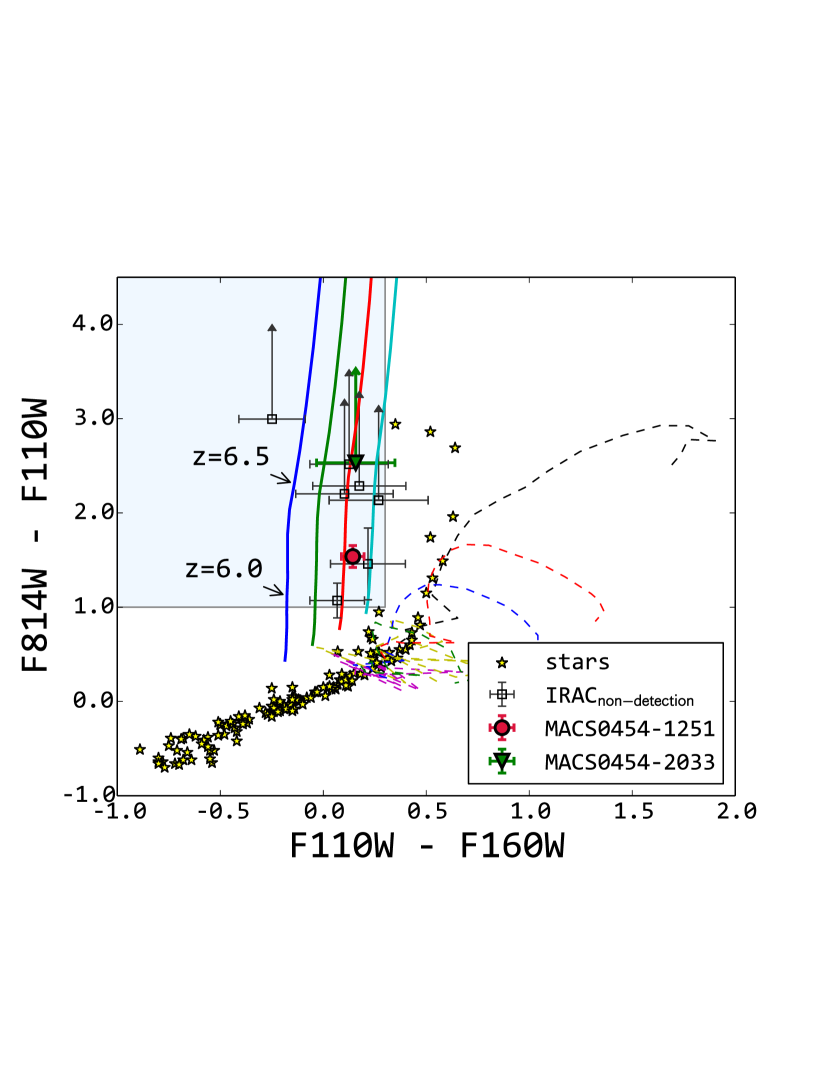
For the two galaxy clusters that are not in the CLASH sample (MACS0454 and RCS2327), we design our own selection criteria for galaxy candidates. For MACS0454, we have HST imaging data in F555W, F775W, F814W, F850LP, F110W, and F160W, although the images in F775W and F850LP are shallower than the other filters and we use both filters only for rejection of low- interlopers. We use the following criteria to select galaxy candidates (F814W-dropouts):
| (5) |
We show the HST color-color diagram of the F814W-dropout selection in Figure 2. A total of ten sources satisfy the color and S/N cuts listed above; among them, MACS0454-1251 and MAC0454-1817 are detected in at least one IRAC channel.
Because we have only one filter redward of F110W, we refrain from searching for F110W-dropouts in MACS0454 as it would yield objects detected in only one HST filter.
3.3. RCS2327
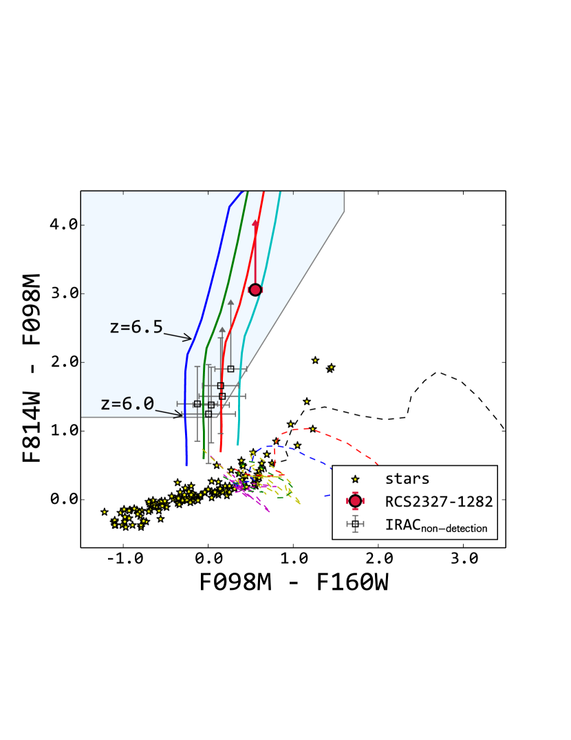
For RCS2327, we have deep HST images in F435W, F814W, F098M, F125W, and F160W, so we use the following criteria for galaxy candidates (F814W-dropouts):
| (6) |
When the in F814W is less than unity, we use its flux limit to calculate colors. We demonstrate the F814W-dropout selection from RCS2327 in Figure 3, and six sources pass the above color and signal-to-noise cuts. One of the six sources, RCS2327-1218, is detected in both IRAC channels. In addition to the above criteria, we also use the criteria similar to the BoRG survey (Trenti et al. 2011) to search for galaxy candidates:
| (7) |
and when the in F098M is less than unity, we use its flux limit to calculate colors. The F098M-dropout search yields no galaxy candidate, so we find a total of one galaxy candidate with IRAC detections at from RCS2327 (see also Hoag et al. 2015 for more details on the dropout search in RCS2327).
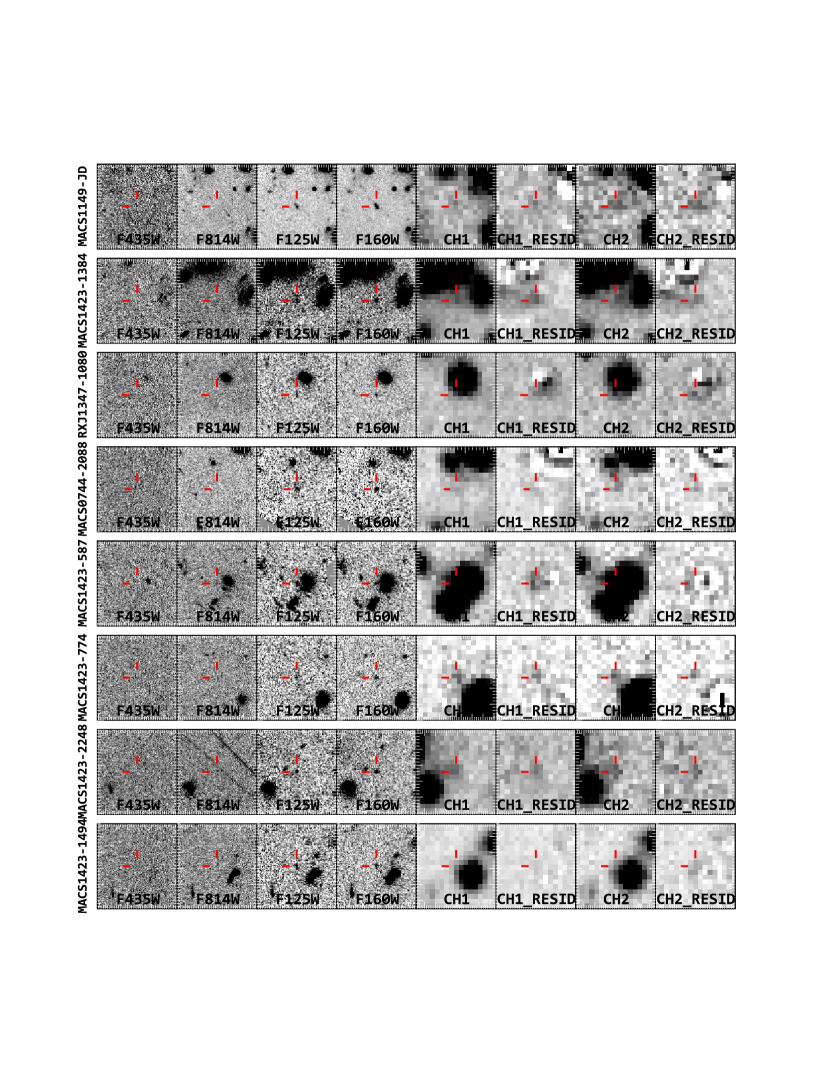
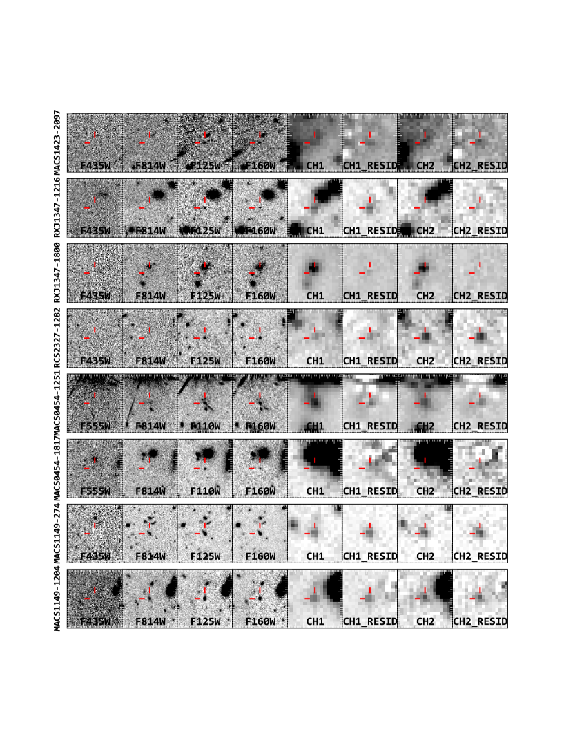
To summarize, we find a total of 69 LBG candidates at from 9 clusters in SURFS UP; 17 of them have IRAC detections in at least one channel. Figure 4 shows the cutouts of the 16 IRAC-detected LBG candidate in HST and Spitzer images (one candiate was reported by Ryan et al. 2014). We also report the IRAC photometry for the entire sample in Table 3. We use the simulated IRAC magnitude errors for MACS1423-1384, MACS1423-587, MACS0744-2088, MACS1423-2097, and MACS0454-1817, because we find that T-PHOT likely underestimates their IRAC magnitude errors from the simulations. We keep MACS1423-1384 in our sample because it has a nominal detection in ch2 from T-PHOT, although the simulated magnitude error suggests that the additional flux error due to crowding reduces it to a detection in ch2.
4. Spectroscopic Observations
We report the detection of two likely Ly emitters among our sample with DEIMOS (Faber et al. 2003) on the Keck II telescope. The DEIMOS observation is part of a larger campaign to systematically target lensed high- galaxies behind strong-lensing galaxy clusters with DEIMOS and MOSFIRE (McLean et al. 2010, 2012) on Keck.We observed six cluster fields between 2013 April and 2014 August and targeted 9 out of 17 high- galaxy candidates in Table 3 with DEIMOS. Which galaxy candidates were observed with DEIMOS and MOSFIRE are indicated in Table 3. The DEIMOS data were reduced using the standard DEEP2 spec2d pipeline slightly modified to reduce the data observed also with 600 l/mm and 830 l/mm gratings (Lemaux et al. 2009; Newman et al. 2013). We focus here on the two galaxies (RXJ1347-1216 and MACS0454-1251) that have line detections; we will present the full spectroscopic survey (with both DEIMOS and MOSFIRE) and the line flux limits for the non-detections in a future work. In addition to the Keck observations, 13 of the 17 galaxy candidates in Table 3 are also observed by the Grism Lens-Amplified Survey from Space (GLASS; HST GO-13459; PI: Treu) program; the spectroscopic constraints on Ly emission from the HST grism data will be presented by Schmidt et al., 2015 (in preparation).
Below we discuss the two galaxy candidates with robust line detections and the likelihood that they are Ly emitters at and .
4.1. RXJ1347-1216
We selected this object as a LBG candidate for spectroscopic follow-up on April 3 2013 and May 26 2014. This source was also selected by both Smit et al. (2014) and Bradley et al. (2014) as a LBG with high [OIII]H equivalent widths (Å rest frame). We used the 830 l/mm grating in the 2013 run and the 1200 l/mm grating in the 2014 run, and the total integration times are roughly 6000 and 7200 seconds, respectively. We had good (but not photometric) conditions with seeing in the 2013 run, but the conditions were highly variable in the 2014 run. Therefore, we only present the line flux measurements from the 2013 run, though the line was detected significantly in both runs.
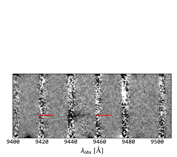
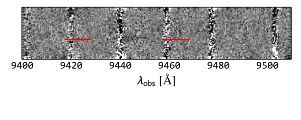
In Figure 6 we show the two-dimensional spectra of RXJ1347-1216 from both observation runs (in the top and middle panels) and the combined one-dimensional spectrum (in the bottom panel). We detect an extended emission feature with FWHM 16.5 Å in the 2013 run, and although the blue side of the feature is severely contaminated by sky line residual, its asymetric profile with a tail to the red side of the spectrum strongly suggests that it is Ly. Using the centroid of the sky line residual at 9439Å as the peak of of line profile, we determine its Ly redshift as (the uncertainty corresponds to the width of the sky line residual). The Ly redshift is in excellent agreement with its photometric redshift , lending additional support to the identification of the Ly feature.
The emission feature is also independently detected at in the GLASS grism data at Å. With the grism spectra in both G102 and G141, one can test the possibility of this feature being an [OII] doublet (, ) at by looking for the [OIII] line at m. For a typical star forming galaxy, the line ratio [OIII]/[OII] should be at least (Jones et al. 2015), and the [OIII]/[OII] ratio is even higher for low-metallicity galaxies (e.g., Maiolino et al. 2008). Assuming the detected line in DEIMOS is [OII] at , HST G141 grism data imply a upper limit on [OIII]/[OII] , which is highly unlikely for a star forming galaxy (Schmidt et al., 2015). Therefore, we conclude that the HST grism data also strongly support the Ly interpretation of this emission line.
We perform line flux measurements from the DEIMOS data obtained during the 2013 run (with the 830 l/mm grating) following the procedure outlined in Section 2.4 of Lemaux et al. (2009). In short, we place two filters of width 20Å on both sides of the emission line that are free of spectral features and sky line residuals to measure the background, and a central filter encompassing the emission line to measure the integrated flux. The background, which is fit to a linear function, is then subtracted from the integrated line flux. We perform spectrophotometric calibration of the DEIMOS data using two other compact sources (with half-light radii as measured from the F775W image) on the same mask with continuum detection in the following manner: for each object, the combination of slit loss and loss due to clouds was determined by calculating a spectral magnitude, done by correcting each DEIMOS spectrum for spectral response and atmospheric extinction and convolving the F775W filter curve with the resulting spectra, and comparing this value with the magnitude measured in the HST image. The ratio of the flux densities for each of the two sources is calculated and averaged to estimate the total spectral loss for this mask, which is then applied to RXJ1347-1216 assuming a similar half-light radius for this object. The reason for this assumption is, though the half-light radius of RXJ1347-1216 is smaller (), which would, in principle, mean less slit loss, the size of the Ly nebula is known to far exceed the size of the UV continuum region (e.g., Wisotzki et al. 2015). For the two sources on the mask with which we performed the flux calibration, the total measured throughput of the slit was 40%, lower than the 60% expected for sources of this size (if they are symmetric), suggesting at least some departure from a photometric night.
Using the above procedure, we measure the line flux from the 830 l/mm data to be , which translates into a Ly luminosity of . We do not detect continuum in the spectrum, so we estimate the rest-frame Ly equivalent width using the object’s broadband magnitude in F105W (on the red side of Ly) to be Å. The equivalent width uncertainty include the Poisson noise in the central filter encompassing the sky line residual, the uncertainty in the continuum, and the uncertainty in DEIMOS absolute flux calibration.
We note that our measured Ly line flux from DEIMOS data is roughly a factor of 3 lower than that measured from the HST grism data, which is (Schmidt et al., 2015, ApJ, in press). The difference in the line flux measurements could be due to the following factors: (1) our DEIMOS data are shallower than the HST grism data ( hours of total integration time in the 2013 mask, versus orbits of HST integration time in G102 grism), with the difference in depths leading to differences in the spatial and extent of the emission detected above the noise in each observation, which impacts the total integrated line flux; (2) we might still underestimate the Ly slit loss because the true extent of the Ly-emitting region is much larger than the continuum-emitting region, while the HST slitless grism recovers more of the Ly flux; (3) there is a sky line coincident with the peak wavelength of the Ly emission in the DEIMOS data which appears slightly over-subtracted that serves to slightly lower the measured line flux; and (4) there could also be issues with contamination subtraction in the HST grism data, although it is unclear which direction it biases line flux measurement. We do expect the ground-based line flux measurement to be a lower limit to the space-based measurement, which is consistent with the measured values from DEIMOS and from HST grism data.
We also measure the inverse line asymmetry as defined in Lemaux et al. (2009), and the line’s inverse asymmetry value () is well within the range () typical for convincing Ly emission.
Using Ly line flux, one can also infer a star formation rate following Lemaux et al. (2009). The inferred star formation rate is strictly a lower limit, because our conversion assumes no attenuation of Ly photons by dust or neutral hydrogen. The inferred star formation rate is , consistent with being a lower limit to the value we derive from SED fitting in Section 5, . The Ly-inferred star formation rate roughly yields a Ly escape fraction of %.
4.2. MACS0454-1251
We observed MACS0454 with DEIMOS on November 28 and 29, 2014 using the 1200 l/mm grating on both nights. The total exposure time for this mask is 7200s. We also reduce the DEIMOS data and extract one-dimensional spectrum following the procedure in Lemaux et al. (2009), in the same way as RXJ1347-1216.
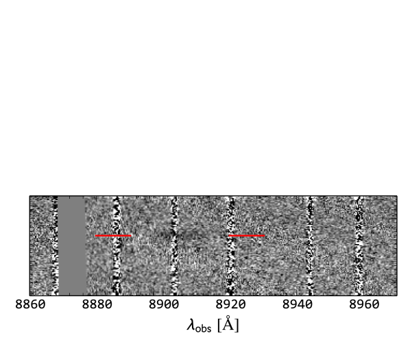
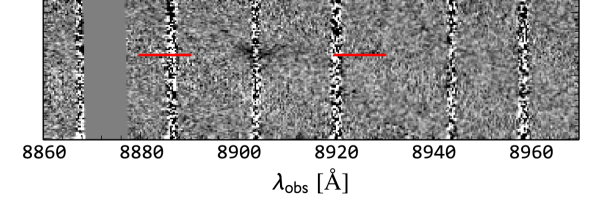
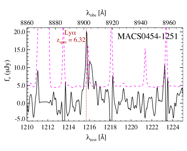
We show the reduced two-dimensional spectra of MACS0454-1251 in Figure 7, and an extended emission feature is clearly detected on both nights. However, a bright sky line residual cuts through the middle of the emission feature in the spectral direction and makes the line interpretation ambiguous. Given the width of the emission line, it could be either Ly at or [OII] at , but the sky line residual makes it difficult to either confirm or rule out Ly or [OII] based on line shape alone. However, as we will show in Section 5.2, this line is more likely to be Ly than [OII] because its HST fluxes (and upper limits) are much better fit by a galaxy template at than at (Section 5.2), and its photometric redshift probability density function has very a low probability at (see the curve in Figure 10). We measure the line fluxes from both nights to be (first night) and (second night), and these translate to Ly luminosities of (first night) and (second night). From the line fluxes, we estimate its rest-frame equivalent widths (assuming Ly) using the continuum on the red side of Ly (estimated from its F110W flux density) from both nights to be Å and Å. We also infer star formation rate lower limits to be (first night) and (second night) based on Ly fluxes, also fully consistent with being lower limits to the value derived from SED fitting in Section 5, . The Ly-inferred star formation rate also roughly corresponds to an escape fraction of % for Ly photons.
The inverse asymmetry value measured for the one-dimensional emission feature is 0.5 for both masks, consistent with the values typical for Ly. However, the line asymmetry estimate is less reliable than that of RXJ1347-1216 because we have to mask the over-subtracted skyline near the central wavelength of the emission feature. Based on the object’s photometric information and line asymmetry measurements, we identify this source as a Ly emitter at , although we are less confident with this Ly interpretation than we are with RXJ1347-1216. MACS0454 is not in the GLASS sample, so we are unable to cross check our measurements with HST grism data.
5. Redshift and Spectral Energy Distribution Modeling
In this section, we present our stellar population modeling of the IRAC-detected, galaxy candidates using broadband photometry. We present the modeling procedure in Section 5.1, the modeling results in Section 5.2, and we discuss the sources of bias and uncertainty in Section 5.3.
5.1. Modeling Procedure
For photometric redshift and stellar population modeling, we use the photometric redshift code EAZY (Brammer et al. 2008) with stellar population templates from Bruzual & Charlot (2003, BC03) with Chabrier (2003) initial mass function (IMF) between and and a metallicity of . There is very little direct observational evidence for galaxy metallicity at , but limited results so far suggest that the majority of them have sub-solar metallicity (Maiolino et al. 2008); we choose for easy comparison with other works. The galaxy templates are generated assuming an exponentially declining star formation history with -folding time ranging from and Gyr, and ages of the stellar population range from Myr to Gyr. For each combination of age and , we implement galaxy internal dust attenuation using the Calzetti et al. (2000) prescription, with the reddening parameter ranging from to mag to include potential low- dusty galaxy solutions. The grid we use have a step size of mag from to mag and a step size of mag from to mag. We also use the stellar templates from the photometric code Le Phare (Ilbert et al. 2006)999The fit using stellar templates is still done using EAZY, only the templates are from Le Phare. in the fitting to check if stellar templates provide significantly better fits.
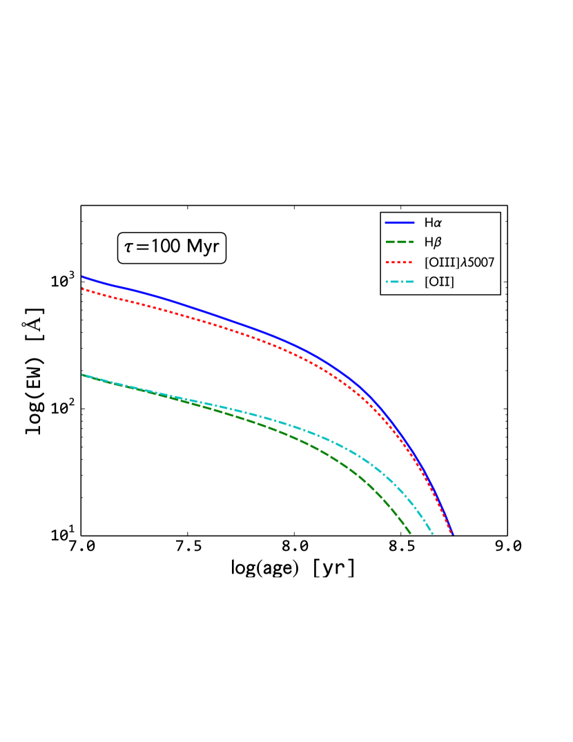
Recent studies have shown that for some galaxy candidates, strong nebular emission lines contribute significantly to broadband fluxes and therefore influence the inferred galaxy properties (e.g., Schaerer & De Barros 2010; Smit et al. 2014). Therefore, we use galaxy templates that include nebular emission lines in the modeling. In order to calculate the expected line fluxes for a given BC03 galaxy template, we calculate the integrated Lyman continuum flux (before dust attenuation) and use the relation from Leitherer & Heckman (1995) to calculate the expected fluxes from hydrogen recombination lines (mainly H, H, Pa, and Br) while assuming the Lyman continuum escape fraction to be zero. Non-zero Lyman continuum escape fraction will reduce the strength of optical nebular emission lines (see Inoue 2011 and Salmon et al. 2015). We then use the tabulated line ratios between H and the metal lines from Anders & Alvensleben (2003) to calculate the metal line fluxes for a metallicity of . For templates with dust attenuation, we include the dust attenuation effects after adding nebular emission lines. The resultant equivalent widths as a function of galaxy age, for Myr and , are shown in Figure 8, in agreement with Leitherer & Heckman (1995).
In addition to nebular emission lines, we also include nebular continuum emission that account for the bound-free emission of HI and HeI as well as the two-photon emission of hydrogen from the 2s level. We follow the prescription in Krueger et al. (1995) (their equations 7 and 8) to calculate the nebular continuum flux as a function of Lyman continuum photon density, and we calculate the emission coefficients using the methods in Brown & Mathews (1970) and Nussbaumer & Schmutz (1984)101010The fitting formula in Nussbaumer & Schmutz (1984) is crucial to calculate the two-photon continuum emission between rest-frame 1216Å and 2431Å, where two-photon emission dominates the nebular continuum.. Nebular continuum emission could be an important component for very young (Myr) starbursts and can contribute up to of the total continuum just blueward of the rest-frame 4000Å break. Nebular continuum emission also makes the rest-frame UV slope redder than expected from stars alone (Schaerer & De Barros 2010).
We do not include Ly in our galaxy templates. Strong Ly emission could affect the LBG color selection by changing the rest-frame UV broadband colors and could affect the derived physical properties from SED fitting (Schaerer et al. 2011; De Barros et al. 2014). But Ly photons suffer from complicated radiative transfer processes and does not show tight correlations with the stellar population properties, so for simplicity we do not include Ly emission in our modeling.
Strong gravitational lensing boosts galaxy fluxes and increases the apparent SFR and stellar mass. To calculate the unlensed SFR and stellar mass, we use the magnification factor estimated from the cluster mass models for each galaxy candidate at its redshift. We generate our own models for MACS1149, MACS0717, MACS0454, RXJ1347, and RCS2327, following the procedures outlined in Bradač et al. (2005, 2009). In short, we constrain the gravitational potential on a mesh grid within a galaxy cluster field via minimization, and we adaptively use denser pixel grids near the core(s) of the cluster and around multiple images. We find the minimum values by iteratively solving a set of linearized equations that satisfy , where is the gravitational potential in the th dimension. We then produce the magnification () map from the best-fit gravitational potential map. For the rest of the clusters in our sample (MACS1423, MACS2129, and MACS0744), we use the public PIEMD-eNFW111111PIEMD-eNFW models use pseudo-isothermal elliptical mass distributions for galaxies and elliptical NFW profiles for dark matter. models by Zitrin et al. (2013).121212These models are made public as high-end science products of the CLASH program; http://archive.stsci.edu/prepds/clash/. The magnification factors (and their errors) are estimated at the galaxy candidate positions from the magnification maps except for MACS1423-587, MACS1423-774, MACS1423-2248, and RXJ1347-1800 (which have so we estimate their from the magnification map.)
| Object ID | aa is the photometric redshift using BC03 galaxy templates except for RXJ1347-1216 and MACS0454-1251, for which we identify Ly emission at and , respectively. | bbLensing magnification factor estimated from the galaxy cluster mass models mentioned in Section 5.1. For MACS1423-587, MACS1423-774, MACS1423-2248, and RXJ1347-1800, we estimate their from the magnification map at . | ccThe intrinsic stellar mass and SFR assuming . To use a different magnification factor , simply use , where is the best magnification factor we adopt for each object. When the best-fit SFR is zero, we report the 68% upper limit. | SFRccThe intrinsic stellar mass and SFR assuming . To use a different magnification factor , simply use , where is the best magnification factor we adopt for each object. When the best-fit SFR is zero, we report the 68% upper limit. | AgeddTime since the onset of star formation. For the sources with best-fit age equal to 10 Myr, the youngest template allowed in our models, we report the 68% upper limit of the age from Monte Carlo simulations. | sSFReeHas Ly detection at . | hhThe best-fit color excess of the stellar emission from our SED modeling. The dust attenuation at rest-frame Å can be calculated using the dust attenuation curve from Calzetti et al. (2000) as . | iiMeasured rest-frame UV slope from HST/WFC3 broadband fluxes, assuming the candidates are at . We do not measure for MACS1423-587, MACS1423-774, MACS1423-2248, and RXJ1347-1800 because they have . We also do not measure for MACS1149-JD because it has only 1 filter (F160W) that samples the rest-frame UV continuum. | kkRest-frame 1600 Å absolute magnitude assuming and . |
|---|---|---|---|---|---|---|---|---|---|
| () | () | (Myr) | (Gyr-1) | (mag) | (mag) | ||||
| F125W-dropouts (; at from Bouwens et al. 2015) | |||||||||
| MACS1149-JD | |||||||||
| F105W-dropouts (; at from Bouwens et al. 2015) | |||||||||
| RXJ1347-1080 | |||||||||
| MACS1423-1384 | |||||||||
| F850LP-dropouts (; from Bouwens et al. 2015) | |||||||||
| MACS1423-1494 | |||||||||
| MACS0744-2088 | |||||||||
| RXJ1347-1216ggAll fits are performed at , the Ly redshift. The confidence intervals reflect the maximal range returned from the simulations because the distributions for this object are highly skewed. | |||||||||
| MACS1423-2097 | |||||||||
| Bullet-3llFirst reported by Ryan et al. (2014); included here for completeness. | |||||||||
| MACS1423-587 | |||||||||
| RXJ1347-1800 | |||||||||
| MACS1423-774 | |||||||||
| MACS1423-2248 | |||||||||
| F814W-dropouts (; from Bouwens et al. 2015) | |||||||||
| RCS2327-1282 | |||||||||
| MACS0454-1817 | |||||||||
| MACS0454-1251 | |||||||||
| MACS0454-1251jjAll fits are performed at , its Ly redshift. | |||||||||
| F775W-dropouts (; from Bouwens et al. 2015) | |||||||||
| MACS1149-274 | |||||||||
| MACS1149-1204 | |||||||||
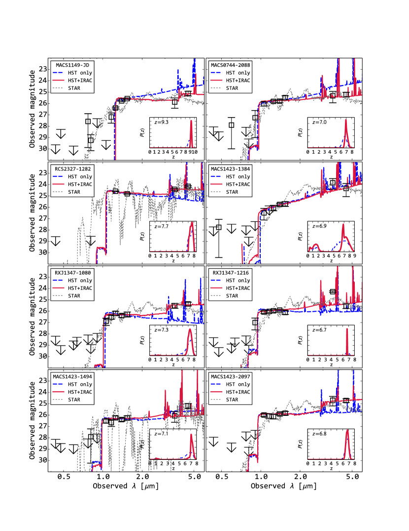
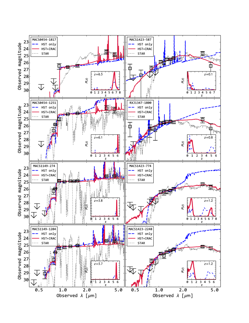
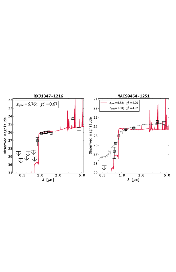
5.2. Modeling Results
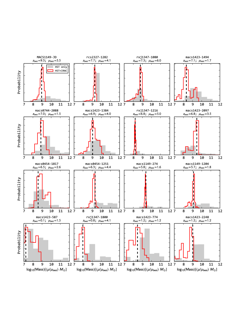
We list the best-fit galaxy properties in Table 4 and show the best-fit templates and the photometric redshift probability density function (while allowing redshift to float) in Figures 9 and 10. For each galaxy candidate, we estimate the statistical uncertainties of stellar population properties using Monte Carlo simulations: we perturb the photometry within the errors (assuming Gaussian flux errors), re-fit with the same set of galaxy templates, and collected the distributions of each best-fit property. We only perturb the fluxes where . For upper limits, we do not perturb the fluxes in our simulations. The systematic errors related to assumptions in initial mass function, galaxy metallicity, and the functional form of star formation history are not represented by the error bars. We show the distributions from Monte Carlo simulations for stellar mass, star formation rate (SFR), and stellar population age in Appendix A. From these distributions, we derive the confidence intervals that bracket % of the total probability in Table 4. The error bars do not include uncertainties in .
We also show the best-fit galaxy properties for RXJ1347-1216 and MACS0454-1251, the two galaxies that we have line detections from DEIMOS data (see Section 4), when we fix their redshifts at their Ly redshifts in Figure 11 (assuming both lines are Ly). For RXJ1347-1216, its photometric redshift is already sharply peaked at , so the best-fit template and physical properties do not change after fixing its redshift at the Ly redshift. On the other hand, MACS0454-1251 has slightly different best-fit photometric redshift and Ly redshift, and we also list its best-fit properties at in Table 4. We also show the best-fit template at in Figure 11 if the detected emission line is [OII] instead of Ly and see that the solution has a higher () than the solution (). The likelihood ratio of these two fits, calculated using the total as , suggests that the model is times more likely than the model.
The best-fit stellar masses in our sample range from to after correcting for magnification by the foreground clusters and excluding the interlopers. The stellar masses inferred from SED fitting have smaller statistical errors when HST fluxes are combined with IRAC fluxes because of the constraints on rest-frame optical emission from IRAC. We show the range of stellar mass from our Monte Carlo simulations in the Appendix (Figure 15), and we find that including IRAC fluxes tighten up the possible range of stellar mass for every object. We also see that the range of stellar mass spanned by our IRAC-detected sample are not necessarily at the high-mass end of the observed (Gonzalez et al. 2011) and simulated (Katsianis et al. 2015) stellar mass functions at . In fact, the IRAC color for several of our galaxy candidates (e.g., RXJ1347-1216) suggest extremely young stellar population ages (Myr) and large equivalent widths from nebular emission lines. For these sources, stellar continuum emission might not dominate the observed IRAC fluxes, hence their true stellar masses depend sensitively on the equivalent widths of nebular emission lines. This demonstrates the combined power of strong gravitational lensing and deep IRAC images that allows one to measure the stellar mass of galaxies further down the stellar mass function.
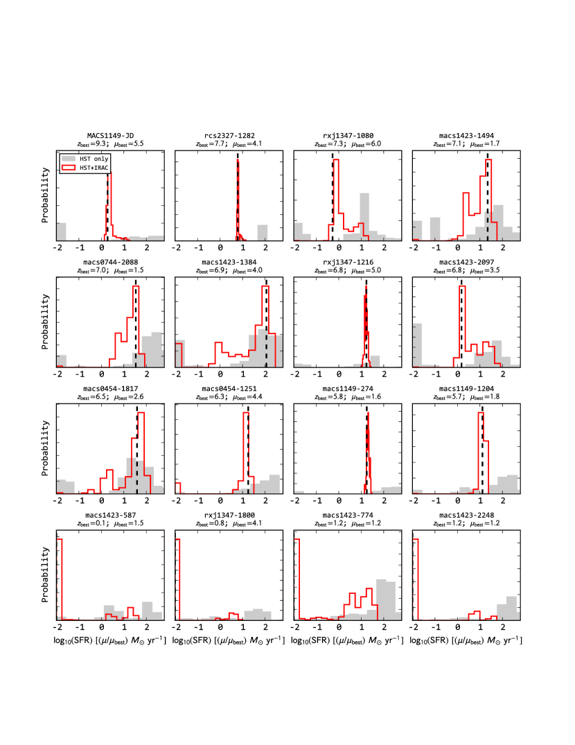
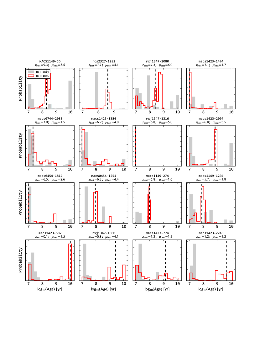
On the other hand, the SFRs and stellar population ages are not necessarily well constrained by SED fitting even when IRAC fluxes are included (see Figures 16 and 17 in the Appendix). The SFRs of high- galaxies are often calculated from their rest-frame UV fluxes (after correcting for dust attenuation), and these are often the only constraints available from observations. However, the UV-derived SFR depends critically on the amount of dust attenuation inside each galaxy, and the effect of dust on the rest-frame UV color is degenerate with the effect of stellar population age. Furthermore, UV-derived SFRs probe the star formation activity over the past Myr, so it could underestimate the instantaneous SFR if the stellar population is younger than ; for these systems, nebular emission line fluxes (e.g., H or [OII]) are better proxies for SFRs (Kennicutt 1998). We consider SFRs and stellar population ages more poorly constrained compared with stellar mass, and we will discuss the degeneracies in SED fitting in Section 5.3.
IRAC fluxes also reveal four interlopers from our sample — MACS1423-587, MACS1423-774, MACS1423-2248, and RXJ1347-1800 — as shown in the three bottom-right panels in Figure 10. All four sources have significant integrated probabilities at when only HST photometry is used in the fitting, but the addition of their IRAC fluxes pushes their photometric redshifts down to , suggesting that the observed breaks between F850LP and F105W are more likely the rest-frame Å break instead of the Ly break. This demonstrates the value of IRAC detections in discriminating between genuine galaxies and lower- interlopers.
In Figure 9 and 10 we also show the best fit stellar templates from Le Phare. Most of the sources are better fit by galaxy templates than by stellar templates, although there is only one case, RXJ1347-1800, where both templates provide similarly good fits ( for galaxy templates and for stellar templates). For all the galaxy candidates, their best-fit stellar templates are either brown dwarfs or low-mass stars from Chabrier & Baraffe (2000). We also check if our sample contains X-ray detected sources that could have significant contributions from AGNs and we do not find evidence that any of our galaxy candidates have AGNs. However, low-level AGN activities are still possible, and the stellar population properties we infer from SED modeling will depend on how much (if any) AGN contribution there is to their broadband fluxes.
5.3. Modeling Biases and Uncertainties
The biases and uncertainties of SED fitting are well documented in the literature (e.g., Papovich et al. 2001; Lee et al. 2009), and most sources of systematic errors come from model assumptions. In general, stellar mass has the smallest systematic errors ( dex), but uncertainties in galaxy star formation history can lead to large biases in galaxy age and star formation rate (Lee et al. 2009). In additional to the usual culprits of systematic errors (e.g., star formation history, initial mass function), another important source of systematic error is the nebular emission line ratios. We find that nebular emission line contributions to broadband fluxes are important for a subset of our sample, but direct observational constraints of rest-frame optical nebular emission line ratios of galaxies will not arrive until the launch of JWST. Uncertainties in the amount of dust attenuation also complicates the interpretation of the best-fit parameters, as we demonstrate below.
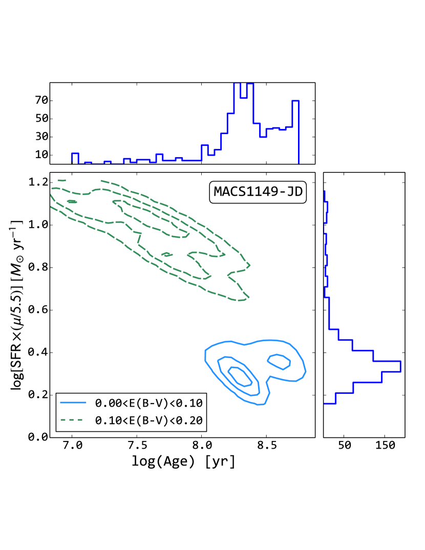
We use MACS1149-JD to show how uncertainties in dust attenuation can lead to uncertainties in star formation rate in Figure 12. We estimate the number density contours from our Monte Carlo simulations (with 1000 realizations) when IRAC fluxes are included in the modeling. We show the number density contour of each value in the central panel and the marginalized histograms for galaxy age (on top) and star formation rate (on the right). The star formation rate histogram shows a single peak at assuming a magnification factor of , but there is a long tail to higher star formation rates that extends one order of magnitude. The long tail in star formation rate corresponds to higher dust attenuation templates (; green dashed contours in the central panel) as opposed to the peak of the histogram (; solid blue contours in the central panel). We note that because of the high photometric redshift of MACS1149-JD (), its UV continuum between rest-frame and Å is not well sampled by HST and IRAC photometry; the addition of -band photometry should help constrain the amount of dust attenuation inside this galaxy.
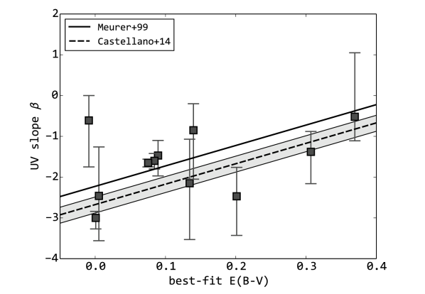
As a model-independent check on the inferred dust attenuation, we measure the rest-frame UV slope for each galaxy candidate and list the values in Table 4. We can only measure when a galaxy candidate has at least two filters sampling the UV continuum (between rest-frame and Å); therefore, we do not measure for MACS1149-JD (which only has F160W that samples UV continuum) and for MACS1423-587, RXJ1347-1800, MACS1423-774, and MACS1423-2248 (which have photometric redshifts ). We measure by using a power-law spectrum , convolving the spectrum with the filter curves that sample the UV continuum, and finding the that best matches the observed fluxes. The uncertainties are quantified in bootstrap Monte Carlo simulations, and we show the values from SED fitting v.s. in Figure 13.
In Figure 13, we also show the expected values of given values of using two different empirical calibrations. To calculate the expected , we use the Calzetti et al. (2000) dust attenuation law to calculate the amount of dust attenuation at rest-frame 1600Å from : . Then we use the relation between and from Meurer et al. (1999) (for solar metallicity; ) and Castellano et al. (2014) (for sub-solar metallicity; ) to calculate the expected . We show the Meurer et al. (1999) relation as a solid line and the Castellano et al. (2014) relation as a dashed line in Figure 13. The scatter of the measured of our sample is larger than the difference between the two empirical calibrations, but the distribution is roughly consistent with both calibrations. The agreement means that the values derived from SED fitting is not strongly biased on average, but the large scatter also suggests that for each individual galaxy, the dust attenuation is still poorly constrained.
6. IRAC Colors and Strong Nebular Emission Lines
Recent works suggest that at least in a subset of high- galaxies, strong nebular emission lines (most notably H, H, [OIII] , and [OII] ) with rest-frame equivalent widths Å or higher contribute significantly to their IRAC fluxes (e.g., Shim et al. 2011; Schaerer & De Barros 2009; De Barros et al. 2014; Smit et al. 2014). The galaxies with extreme nebular emission line strengths are most likely starbursts younger than Myr; such galaxies are also being found in increasing numbers at – (e.g., van der Wel et al. 2011; Atek et al. 2011). If a large number of such galaxies exist at , strong nebular emission lines in the rest-frame UV/optical wavelengths need to be included in the stellar population modeling.
Within certain redshift ranges, unusual IRAC colors can be tell-tale signs of strong nebular emission lines. Shim et al. (2011) identified 47 galaxies at that have bluer colors than those expected from stellar continuum alone, and they categorized these galaxies as H emitters because the SED bumps at m are likely due to strong H emission. More recently, Smit et al. (2014) and Smit et al. (2015) presented – galaxy candidates with unusually blue colors as evidence for strong contributions from [OIII] and H to the m fluxes. The colors of these peculiar objects usually can only be reproduced with model SEDs that include strong nebular emission lines.
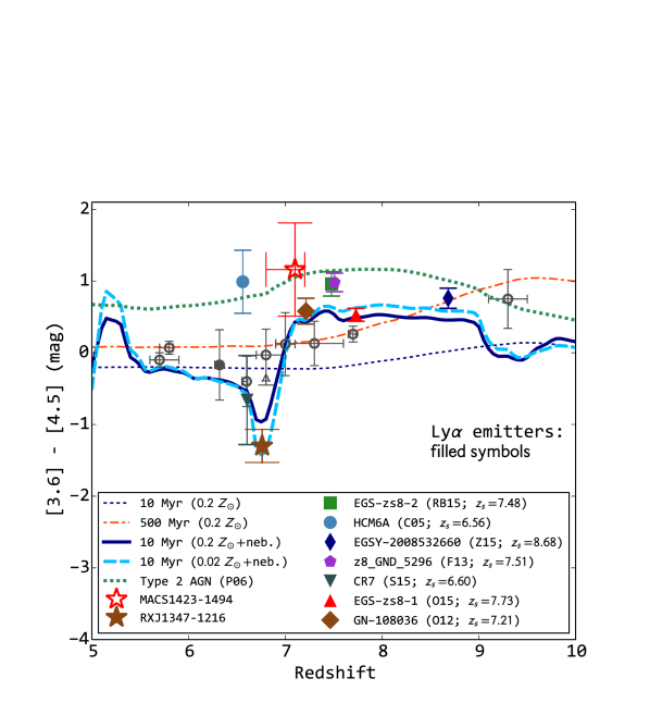
In Figure 14, we compare the IRAC colors of our sample with a range of model predictions. We use our fiducial SED model (BC03) to generate the redshift evolution of color at 500 Myr old without nebular emission lines (thin dot-dashed curve, roughly the age of the universe at ), 10 Myr old without nebular emission lines (thin dotted curve), and 10 Myr old with nebular emission lines (thick solid curve). The 10 Myr old model with nebular emission lines have equivalent widths Å, Å, and Å for H, H, and [OIII], respectively. Here we assume the star formation -folding time scale to be 100 Myr, but the color does not change significantly when different values of are used.
The most prominent feature in Figure 14 is the “dip” in for a 10 Myr old starburst with nebular emission lines at due to the contributions from [OIII] and H — the same feature that Smit et al. (2014) utilized to identify strong nebular emission line objects within . In our sample, only RXJ1347-1216 has a photometric redshift and a very blue color. This source has a best-fit age of Myr, the youngest age included in our templates. Extremely young stellar populations are expected to generate a large number of ionizing photons, so if these sources are indeed Myr old starbursts, they might also have high Ly luminosities around star forming regions. We already successfully identified one of the three sources (RXJ1347-1216) as a Ly emitter (LAE; see Section 4); we do not identify other sources at with blue color that could also be strong line emitters in our sample.
In Figure 14 we also show the redshift evolution of color for a 10 Myr old, model (thick dashed curve), and it predicts a bluer color at (as blue as mag) than the 10 Myr old, model. The IRAC colors of the model at show better agreements with the three sources mentioned above than the model, which suggests that these sources might have lower metallicities than our fiducial model. We note that the nebular emission line properties of individual galaxies are highly uncertain (and are sensitive to metallicity), so any constraint on metallicity is preliminary.
Our fiducial galaxy SED models also predict that young starbursts with strong nebular emission lines should have red colors at . In this redshift range, [OII] and [OIII] move into IRAC ch1 and ch2, respectively, and the combined [OIII]H line flux is expected to be times higher than [O II] in our implementation (Anders & Alvensleben 2003); the expected color reaches mag within . MACS1423-1494 () has a photometric redshift and measured color that are close to the model prediction, although its red color is hard to reconcile even with the 10 Myr old galaxy model. Based on its photometric redshift and unusually red color (it is also best-fit by a 10 Myr old galaxy SED), we identify this source as another prime candidate for Ly emission. We note that Ly photons are subject to complicated radiation transfer effects both inside and outside of galaxies, so it is far from guaranteed that these sources will have detectable Ly emission. But they are likely LAE candidates (compared with other high- galaxies) based on their photometric redshifts and IRAC colors.
We also compare our galaxy model-predicted IRAC colors with other LAEs with published IRAC colors in Figure 14. The other LAEs include HCM6A from Hu et al. (2002) (, where is the spectroscopic redshift determined by Ly emission), CR7 from Sobral et al. (2015) (), GN-108036 from Ono et al. (2012) (), EGS-zs8-2 from Roberts-Borsani et al. (2015) (), z8_GND_5296 from Finkelstein et al. (2013) (), EGS-zs8-1 from Oesch et al. (2015) (), and EGSY-2008532660 from Zitrin et al. (2015) (). All of these LAEs have IRAC colors that strongly suggest high nebular emission line equivalent widths (most likely [OIII] and H at this redshift range), because they lie along the curve traced by a dust-free, , 10 Myr stellar population. For example, Finkelstein et al. (2013) argued that the red IRAC color of z8_GND_5296 is due to the galaxy’s strong [OIII]H emission lines in IRAC ch2, and they inferred the [OIII] equivalent width to be 560–640 Å from photometry. The IRAC colors of these LAEs corroborate the recent findings that many galaxies detected at likely have high nebular emission line equivalent widths.
Two notable cases among the group of LAEs in Figure 14 are MACS1423-1494 and HCM6A131313HCM6A was first reported by Hu et al. (2002), and later Chary et al. (2005) published its IRAC fluxes.. HCM6A was found in the vicinity of a massive galaxy cluster Abell 370141414Abell 370 is one of the Hubble Frontier Fields cluster. and has a measured color of mag, significantly redder than the color predicted by a 10 Myr stellar population model at its redshift (). The red color suggests a very high H/([OIII]H) ratio, which is unexpected (but not impossible) for a young, low-metallicity stellar population. In order to explore other possibilities to explain the red colors of both LAEs, we plot the predicted colors of a Type 2 obscured AGN template from Polletta et al. (2007). This obscured AGN template includes a dust attenuation of mag that fits the obscured AGN SW 104409 (; Polletta et al. 2006), and its color trajectory in redshift is shown as a thick dotted curve in Figure 14. Interestingly, the predicted colors of an obscured AGN agrees quite well with the colors of both MACS1423-1494 and HCM6A, and z8_GND_5296 and EGS-zs8-2 also have marginally consistent IRAC colors with this obscured AGN template. If these sources indeed harbor obscured AGNs (like SW 104409), the red colors will be primarily due to large dust attenuation in the rest-frame optical, while the blue rest-frame UV colors come from the scattered light of the central QSO emission. Obscured AGN is an intriguing possibility to consider for these sources, although so far no direct evidence exists that any of these sources have significant flux contributions from an obscured AGN.
To sum up, we identify three sources in our sample at and as likely young starbursts with very strong nebular emission lines based on their IRAC colors. We detect Ly emission in one of them, RXJ1347-1216, during our recent DEIMOS observations, and we plan to follow up all the other three sources for their potential Ly emission.
7. Summary
In this work, we present the constraints on the , IRAC-detected galaxy candidates behind eight strong-lensing galaxy clusters from SURFS UP. Six of the clusters are in the CLASH sample, and two are in the Hubble Frontier Fields sample. We summarize our findings as follows:
-
•
We find a total of 17 galaxy candidates using the Lyman break color selection that have in at least one IRAC channel. The photometric redshifts in our sample range from to , and we identify four galaxy candidates (MACS1423-587, RXJ1347-1800, MACS1423-774, and MACS1423-2248) as likely interlopers after including their IRAC fluxes in the SED modeling. We find the largest number (6) of IRAC-detected galaxy candidates in MACS1423.
-
•
From our Keck spectroscopic observations, we identify one secure Ly emitter at (RXJ1347-1216) and one likely Ly emitter at (MACS0454-1251). The line equivalent widths, assuming they are both Ly, are Å (RXJ1347-1216) and Å (MACS0454-1251, averaged over two nights). We infer lower limits of their star formation rates from their Ly line fluxes and find them to be consistent with the star formation rates from SED fitting.
-
•
We infer the physical properties of our sample galaxies using Bruzual & Charlot (2003) galaxy templates and add nebular emission lines to the templates. Under our SED modeling assumptions (, Chabrier IMF, exponentially decaying star formation history, and nebular line emission), the stellar masses of our sample range from – (excluding the three likely interlopers) when we use the best available magnification factors for each galaxy candidate. The magnification-corrected rest-frame 1600 Å absolute magnitude (; see Table 4) of our sample ranges from to mag. The range of intrinsic UV luminosity probed here is slightly fainter than the knee of UV luminosity functions at , which have between and mag (e.g., Bouwens et al. 2015; Finkelstein et al. 2015), showing that galaxy clusters’ strong lensing power allows us to start probing the more typical UV luminosities. The range of intrinsic stellar mass probed here is also close to the knee of the stellar mass functions at this redshift range (e.g., Gonzalez et al. 2011; Katsianis et al. 2015). Some galaxies in our sample are best fit by extremely young (10 Myr old) templates and others best fit by more evolved (up to 700 Myr old at ) templates, suggesting that the IRAC-detected sample contains both very young galaxies with strong nebular emission lines and more evolved and massive galaxies at .
-
•
From the photometric redshifts and IRAC colors, we identify two galaxy candidates that likely have strong (rest-frame optical) nebular emission lines: RXJ1347-1216 and MACS1423-1494. Both sources are best fit by the youngest (10 Myr old) galaxy templates included in our modeling and are prime targets for spectroscopic observations. We already identified one of them (RXJ1347-1216) as a Ly emitter, and we will target the other two in our future spectroscopic observations. Other galaxies in the sample lie in the part of the redshift–IRAC color space that makes it hard to infer their nebular emission line strengths; namely, they are within the redshift range that both IRAC bands could have contribution from strong nebular emission lines such as [OIII], H, and H, and their IRAC colors may not be very different from those of pure stellar continuum.
The IRAC fluxes provide important information about the galaxies at , because it is the only probe of their rest-frame optical emission that we have at the moment. The IRAC-detected galaxies may not be representative of the entire galaxy population at , but their IRAC colors do provide a more effective way to select spectroscopic targets for redshift confirmation. IRAC fluxes and meaningful upper limits can also distinguish some lower-redshift galaxies from high- dropouts and are important for constructing clean galaxy samples.
We would like to thank the anonymous referee for constructive suggestions that make this work better. We also thank Harry Ferguson, Samuel Schmidt, Chris Fassnacht, Dennis Zaritsky, and Hendrik Hildebrandt for useful discussions and comments on the manuscript. Observations were carried out using Spitzer Space Telescope, which is operated by the Jet Propulsion Laboratory, California Institute of Technology under a contract with NASA. Also based on observations made with the NASA/ESA Hubble Space Telescope, obtained at the Space Telescope Science Institute, which is operated by the Association of Universities for Research in Astronomy, Inc., under NASA contract NAS5-26555 and NNX08AD79G and ESO-VLT telescopes. Support for this work was provided by NASA through a Spitzer award issued by JPL/Caltech. This work was supported by NASA Headquarters under the NASA Earth and Space Science Fellowship Program - Grant ASTRO14F- 0007. We also acknowledge support from HST-AR-13235, HST-GO-13177, and special funding as part of the HST Frontier Fields program conducted by STScI. TS acknowledges support from the German Federal Ministry of Economics and Technology (BMWi) provided through DLR under project 50 OR 1308. TT acknowledges support by the Packard Fellowship. The Dark Cosmology Centre (DARK) is funded by the Danish National Research Foundation.
Appendix A Distributions from Monte Carlo Simulations
Here we show the distributions of stellar mass, star formation rate, and stellar population age (assuming an exponentially declining star formation history with -folding time between and Gyr) in Figures 15, 16, and 17, respectively. In all panels, the distributions from using HST photometry only are shown in gray filled histogram, while the distributions from combining HST and Spitzer photometry are shown in red histogram.
References
- Anders & Alvensleben (2003) Anders, P., & Alvensleben, U. F. v. 2003, A&A, 401, 1063
- Atek et al. (2011) Atek, H., Siana, B., Scarlata, C., et al. 2011, ApJ, 743, 121
- Beckwith et al. (2006) Beckwith, S. V. W., Stiavelli, M., Koekemoer, A. M., et al. 2006, AJ, 132, 1729
- Bertin & Arnouts (1996) Bertin, E., & Arnouts, S. 1996, A&AS, 117, 393
- Bouwens et al. (2011) Bouwens, R. J., Illingworth, G. D., Oesch, P. A., et al. 2011, ApJ, 737, 90
- Bouwens et al. (2015) Bouwens, R. J., Illingworth, G. D., Oesch, P. A., et al. 2015, ApJ, 803, 34
- Bradač et al. (2005) Bradač, M., Schneider, P., Lombardi, M., & Erben, T. 2005, A&A, 437, 39
- Bradač et al. (2009) Bradač, M., Treu, T., Applegate, D., et al. 2009, ApJ, 706, 1201
- Bradač et al. (2014) Bradač, M., Ryan, R., Casertano, S., et al. 2014, ApJ, 785, 108
- Bradley et al. (2012) Bradley, L. D., Trenti, M., Oesch, P. A., et al. 2012, ApJ, 760, 108
- Bradley et al. (2014) Bradley, L. D., Zitrin, A., Coe, D., et al. 2014, ApJ, 792, 76
- Brammer et al. (2008) Brammer, G. B., van Dokkum, P. G., & Coppi, P. 2008, ApJ, 686, 1503
- Brown & Mathews (1970) Brown, R. L., & Mathews, W. G. 1970, ApJ, 160, 939
- Bruzual & Charlot (2003) Bruzual, G., & Charlot, S. 2003, MNRAS, 344, 1000
- Calzetti et al. (2000) Calzetti, D., Armus, L., Bohlin, R. C., et al. 2000, ApJ, 533, 682
- Capak et al. (2011) Capak, P., Mobasher, B., Scoville, N. Z., et al. 2011, ApJ, 730, 68
- Castellano et al. (2014) Castellano, M., Sommariva, V., Fontana, A., et al. 2014, A&A, 566, A19
- Chabrier (2003) Chabrier, G. 2003, PASP, 115, 763
- Chabrier & Baraffe (2000) Chabrier, G., & Baraffe, I. 2000, ARA&A, 38, 337
- Chary et al. (2005) Chary, R.-R., Stern, D., & Eisenhardt, P. 2005, ApJ, 635, L5
- Coleman et al. (1980) Coleman, G. D., Wu, C.-C., & Weedman, D. W. 1980, ApJS, 43, 393
- De Barros et al. (2014) De Barros, S., Schaerer, D., & Stark, D. P. 2014, A&A, 563, A81
- Ellis et al. (2001) Ellis, R., Santos, M. R., Kneib, J.-P., & Kuijken, K. 2001, ApJ, 560, L119
- Eyles et al. (2007) Eyles, L. P., Bunker, A. J., Ellis, R. S., et al. 2007, MNRAS, 374, 910
- Faber et al. (2003) Faber, S. M., Phillips, A. C., Kibrick, R. I., et al. 2003, in Society of Photo-Optical Instrumentation Engineers (SPIE) Conference Series, Vol. 4841, Instrument Design and Performance for Optical/Infrared Ground-based Telescopes, ed. M. Iye & A. F. M. Moorwood, 1657–1669
- Finkelstein et al. (2013) Finkelstein, S. L., Papovich, C. J., Dickinson, M. E., et al. 2013, Nature, 502, 524
- Finkelstein et al. (2015) Finkelstein, S. L., Ryan, Jr., R. E., Papovich, C., et al. 2015, ApJ, 810, 71
- Giallongo et al. (2015) Giallongo, E., Grazian, A., Fiore, F., et al. 2015, A&A, 578, A83
- Giavalisco (2002) Giavalisco, M. 2002, ARA&A, 40, 579
- Gonzalez et al. (2011) Gonzalez, V., Labbé, I., Bouwens, R. J., et al. 2011, ApJ, 735, L34
- Grogin et al. (2011) Grogin, N. A., Kocevski, D. D., Faber, S. M., et al. 2011, ApJS, 197, 35
- Guo et al. (2013) Guo, Y., Ferguson, H. C., Giavalisco, M., et al. 2013, ApJS, 207, 24
- Hoag et al. (2015) Hoag, A., Bradač, M., Huang, K. H., et al. 2015, ApJ, 813, 37
- Hu et al. (2002) Hu, E. M., Cowie, L. L., McMahon, R. G., et al. 2002, ApJ, 568, L75
- Ilbert et al. (2006) Ilbert, O., Arnouts, S., McCracken, H. J., et al. 2006, A&A, 457, 841
- Illingworth et al. (2013) Illingworth, G. D., Magee, D., Oesch, P. A., et al. 2013, ApJS, 209, 6
- Inoue (2011) Inoue, A. K. 2011, MNRAS, 415, 2920
- Jones et al. (2015) Jones, T., Martin, C., & Cooper, M. C. 2015, ApJ, 813, 126
- Katsianis et al. (2015) Katsianis, A., Tescari, E., & Wyithe, J. S. B. 2015, MNRAS, 448, 3001
- Kennicutt (1998) Kennicutt, Jr., R. C. 1998, ARA&A, 36, 189
- Kneib et al. (2004) Kneib, J.-P., Ellis, R. S., Santos, M. R., & Richard, J. 2004, ApJ, 607, 697
- Koekemoer et al. (2011) Koekemoer, A. M., Faber, S. M., Ferguson, H. C., et al. 2011, ApJSupplement, 197, 36
- Koekemoer et al. (2013) Koekemoer, A. M., Ellis, R. S., McLure, R. J., et al. 2013, ApJS, 209, 3
- Krueger et al. (1995) Krueger, H., Fritze-v Alvensleben, U., & Loose, H. H. 1995, A&A, 303, 41
- Labbé et al. (2010) Labbé, I., González, V., Bouwens, R. J., et al. 2010, ApJ, 716, L103
- Labbé et al. (2013) Labbé, I., Oesch, P. A., Bouwens, R. J., et al. 2013, ApJ, 777, L19
- Labbé et al. (2015) Labbé, I., Oesch, P. A., Illingworth, G. D., et al. 2015, ArXiv e-prints
- Laidler et al. (2007) Laidler, V. G., Papovich, C., Grogin, N. A., et al. 2007, PASP, 119, 1325
- Lee et al. (2009) Lee, S.-K., Idzi, R., Ferguson, H. C., et al. 2009, ApJS, 184, 100
- Leitherer & Heckman (1995) Leitherer, C., & Heckman, T. M. 1995, ApJS, 96, 9
- Lemaux et al. (2009) Lemaux, B. C., Lubin, L. M., Sawicki, M., et al. 2009, ApJ, 700, 20
- Maiolino et al. (2008) Maiolino, R., Nagao, T., Grazian, A., et al. 2008, A&A, 488, 463
- McLean et al. (2010) McLean, I. S., Steidel, C. C., Epps, H., et al. 2010, in Society of Photo-Optical Instrumentation Engineers (SPIE) Conference Series, Vol. 7735, Society of Photo-Optical Instrumentation Engineers (SPIE) Conference Series, 1
- McLean et al. (2012) McLean, I. S., Steidel, C. C., Epps, H. W., et al. 2012, in SPIE Astronomical Telescopes + Instrumentation, ed. I. S. McLean, S. K. Ramsay, & H. Takami (SPIE), 84460J
- Merlin et al. (2015) Merlin, E., Fontana, A., Ferguson, H. C., et al. 2015, A&A, 582, A15
- Meurer et al. (1999) Meurer, G. R., Heckman, T. M., & Calzetti, D. 1999, ApJ, 521, 64
- Newman et al. (2013) Newman, J. A., Cooper, M. C., Davis, M., et al. 2013, ApJS, 208, 5
- Nussbaumer & Schmutz (1984) Nussbaumer, H., & Schmutz, W. 1984, A&A, 138, 495
- Oesch et al. (2015) Oesch, P. A., Dokkum, P. G. v., Illingworth, G. D., et al. 2015, ApJ, 804, L30
- Ono et al. (2012) Ono, Y., Ouchi, M., Mobasher, B., et al. 2012, ApJ, 744, 83
- Papovich et al. (2001) Papovich, C. J., Dickinson, M. E., & Ferguson, H. C. 2001, ApJ, 559, 620
- Pickles (1998) Pickles, A. J. 1998, PASP, 110, 863
- Polletta et al. (2007) Polletta, M., Tajer, M., Maraschi, L., et al. 2007, ApJ, 663, 81
- Polletta et al. (2006) Polletta, M. d. C., Wilkes, B. J., Siana, B., et al. 2006, ApJ, 642, 673
- Postman et al. (2012) Postman, M., Coe, D., Benítez, N., et al. 2012, ApJS, 199, 25
- Roberts-Borsani et al. (2015) Roberts-Borsani, G. W., Bouwens, R. J., Oesch, P. A., et al. 2015, eprint arXiv:1506.00854
- Robertson et al. (2010) Robertson, B. E., Ellis, R. S., Dunlop, J. S., McLure, R. J., & Stark, D. P. 2010, Nature, 468, 49
- Ryan et al. (2014) Ryan, Jr., R. E., Gonzalez, A. H., Lemaux, B. C., et al. 2014, ApJ, 786, L4
- Salmon et al. (2015) Salmon, B., Papovich, C., Finkelstein, S. L., et al. 2015, ApJ, 799, 183
- Schaerer & De Barros (2009) Schaerer, D., & De Barros, S. 2009, A&A, 502, 423
- Schaerer & De Barros (2010) —. 2010, A&A, 515, A73
- Schaerer et al. (2011) Schaerer, D., De Barros, S., & Stark, D. P. 2011, A&A, 536, A72
- Schmidt et al. (2014) Schmidt, K. B., Treu, T., Brammer, G. B., et al. 2014, ApJ, 782, L36
- Sharon et al. (2015) Sharon, K., Gladders, M. D., Marrone, D. P., et al. 2015, ApJ, 814, 21
- Shim et al. (2011) Shim, H., Chary, R.-R., Dickinson, M. E., et al. 2011, ApJ, 738, 69
- Smit et al. (2014) Smit, R., Bouwens, R. J., Labbe, I., et al. 2014, ApJ, 784, 58
- Smit et al. (2015) Smit, R., Bouwens, R. J., Franx, M., et al. 2015, ApJ, 801, 122
- Sobral et al. (2015) Sobral, D., Matthee, J., Darvish, B., et al. 2015, ApJ, 808, 139
- Soucail (1990) Soucail, G. 1990, Ap&SS, 170, 283
- Stark et al. (2009) Stark, D. P., Ellis, R. S., Bunker, A., et al. 2009, ApJ, 697, 1493
- Steidel & Hamilton (1993) Steidel, C. C., & Hamilton, D. 1993, AJ, 105, 2017
- Trenti et al. (2011) Trenti, M., Bradley, L. D., Stiavelli, M., et al. 2011, ApJ, 727, L39
- Trenti et al. (2012) —. 2012, ApJ, 746, 55
- Treu et al. (2015) Treu, T., Schmidt, K. B., Brammer, G. B., et al. 2015, ApJ, 812, 114
- van der Wel et al. (2011) van der Wel, A., Straughn, A. N., Rix, H.-W., et al. 2011, ApJ, 742, 111
- Wisotzki et al. (2015) Wisotzki, L., Bacon, R., Blaizot, J., et al. 2015, eprint arXiv:1509.05143
- Yan et al. (2006) Yan, H., Dickinson, M. E., Giavalisco, M., et al. 2006, ApJ, 651, 24
- Yan et al. (2011) Yan, H., Yan, L., Zamojski, M. A., et al. 2011, ApJ, 728, L22
- Zheng et al. (2012) Zheng, W., Postman, M., Zitrin, A., et al. 2012, Nature, 489, 406
- Zheng et al. (2014) Zheng, W., Shu, X., Moustakas, J., et al. 2014, ApJ, 795, 93
- Zitrin et al. (2015) Zitrin, A., Ellis, R. S., Belli, S., & Stark, D. P. 2015, ApJ, 805, L7
- Zitrin et al. (2013) Zitrin, A., Meneghetti, M., Umetsu, K., et al. 2013, ApJ, 762, L30