Non-local bias contribution to third-order galaxy correlations

Abstract

We study halo clustering bias with second- and third-order statistics of halo and matter density fields in the MICE Grand Challenge simulation. We verify that two-point correlations deliver reliable estimates of the linear bias parameters at large scales, while estimations from the variance can be significantly affected by non-linear and possibly non-local contributions to the bias function. Combining three-point auto- and cross-correlations we find, for the first time in configuration space, evidence for the presence of such non-local contributions. These contributions are consistent with predicted second-order non-local effects on the bias functions originating from the dark matter tidal field. Samples of massive haloes show indications of bias (local or non-local) beyond second order. Ignoring non-local bias causes $20-30$% and $5-10$% overestimation of the linear bias from three-point auto- and cross-correlations respectively. We study two third-order bias estimators which are not affected by second-order non-local contributions. One is a combination of three-point auto- and cross- correlation. The other is a combination of third-order one- and two-point cumulants. Both methods deliver accurate bias estimations of the linear bias. Furthermore their estimations of second-order bias agree mutually. Ignoring non-local bias causes higher values of the second-order bias from three-point correlations. Our results demonstrate that third-order statistics can be employed for breaking the growth-bias degeneracy.

1 Introduction

With the increasing amount of data coming from current and future large-scale galaxy surveys, errors on the observed statistical properties of the spatial galaxy distribution are rapidly decreasing. This high level of precision requires at least the same level of accuracy in the modelling of the corresponding observables. An important observable is the growth of large-scale density fluctuations with time, which is sensitive to the universal matter density, the expansion of space as well as to the gravitational interaction of matter at large scales. Measurements of the this growth therefore provide constrains on cosmological parameters (e.g. Ross et al., 2007; Cabré and Gaztañaga, 2009; Song and Percival, 2009; Samushia et al., 2012; Reid et al., 2012; de la Torre et al., 2013), possible deviations from General Relativity (Gaztañaga and Lobo, 2001; Lue et al., 2004) or on alternative phenomenological description for the accelerated expansion, such as the effective field theory (Steigerwald et al., 2014; Piazza et al., 2014). Growth measurements can be undertaken by comparing the second-order correlations $\xi$ of galaxy distributions at different redshifts. A critical aspect of this approach is the bias between the correlations of galaxies and those of the full matter density field. This bias can either be predicted with the peak-background split model (e.g. Bardeen et al., 1986; Cole and Kaiser, 1989; Sheth and Tormen, 1999), or directly determined from observations using weak lensing observables, redshift space distortions or reduced third-order correlations at large scales. The latter method relies on the fact that such third-order correlations are independent of the growth at large scales, but sensitive to the bias. Third-order galaxy correlations therefore have the potential to tighten constrains on cosmological models from observations (e.g. Marín, 2011; Marín et al., 2013). However, how useful third-order correlation are for this purpose depends on the accuracy and the precision of the bias estimations they deliver (e.g. Wu et al., 2010; Eriksen and Gaztañaga, 2015).

The present work is part of a series of papers with which we aim to characterise and understand differences between various bias estimations using the huge volume of the MICE Grand challenge simulation. We thereby assume that galaxies can be associated with dark matter haloes. This analysis includes bias measurements derived from a direct comparison between halo and matter fluctuations (Bel, Hoffmann, Gaztañaga, in preparation) as well as bias predictions from the peak-background split model (Hoffmann et al., 2015a). Continuing this series we now aim at deepening our previous work on the bias from third-order correlations (Hoffmann et al., 2015b).

In this previous work we investigated growth measurements based on bias estimations from third-order halo auto-correlations (halo-halo-halo). Despite the positive and encouraging outcome of this analysis, we pointed out some discrepancies between the first- and second-order bias estimations derived from two different third-order statistics. The first third-order statistics is the reduced three-point correlation function $Q$ (Fry, 1984b). The second one is based on a particular combination (Szapudi, 1998; Bel and Marinoni, 2012) of the skewness $S_{3}$ and the correlator $C_{12}$ (Bernardeau et al., 2002) (referred to as $\tau$ method, Bel and Marinoni, 2012), which correspond to the three-point correlation for triangles with one and two collapsed legs respectively. We found that linear bias estimations from the three-point auto correlations over-estimate the true linear bias (probed by two-point correlations at large scales) by $20$-$30$%. The $\tau$ method delivers accurate linear bias estimations, but with lower precision. Furthermore, its bias estimation become unreliable when samples of massive haloes ($M>10^{14}h^{-1}M_{\odot}$) are considered. Understanding these discrepancies between different bias estimators is crucial for constraining cosmological models with observed third-order galaxy statistics. In the light of previous studies (Manera and Gaztañaga, 2011; Pollack et al., 2012; Chan et al., 2012; Baldauf et al., 2012) we pointed out that such discrepancies might originate from non-linear and/or non-local effects on the different bias estimators. Hence, in the present paper, we focus on the analysis of third-order cross-correlations (halo-matter-matter) to decrease the impact of non-linearities on our bias estimators in order to investigate the extension of the local bias model to a possible non-local component.

We recall the bias expansion, introduced by Fry and Gaztanaga (1993), which assumes a local relation between the density contrast of matter and haloes

$$\delta_{h}=F[\delta_{m}]\simeq\sum_{i=0}^{N}\frac{b_{i}}{i!}\delta_{m}^{i}.$$ (1)

In the above relation we assume that $\delta_{h}$ and $\delta_{m}$ are coarse grain quantities obtained by applying a smoothing process (see Manera and Gaztañaga, 2011; Buchalter and Kamionkowski, 1999, for a discusion of the effect of the smoothing). Inaccuracies of this deterministic relation (equation 1) might arise from tidal forces in the matter field, leading to a non-local contribution in the biasing relation. At second order it can be expressed as

$$\delta_{h}({\bf x})=b_{1}\left\{\delta_{m}({\bf x})+\frac{c_{2}}{2}(\delta_{m}^{2}({\bf x})-\langle\delta_{m}^{2}\rangle)+\frac{\gamma_{2}}{b_{1}}\mathcal{G}_{2}({\bf x})\right\},$$ (2)

where $\gamma_{2}$ represents the non-local bias parameter (Chan et al., 2012; Baldauf et al., 2012). This non-local component depends on the divergence $\theta_{v}$ of the normalised velocity field (${\bf v}/\mathcal{H}/f$)

$$\mathcal{G}_{2}({\bf x})=-\int\beta_{12}\theta_{v}({\bf q}_{1})\theta_{v}({\bf q}_{2})\hat{W}[q_{12}R]e^{i{\bf q}_{12}\cdot{\bf x}}d^{3}{\bf q}_{1}d^{3}{\bf q}_{2},$$ (3)

where $\beta_{12}\equiv 1-\left(\frac{{\bf q}_{1}\cdot{\bf q}_{2}}{q_{1}q_{2}}\right)^{2}$ represents the mode-coupling between density oscillations with wave vectors ${\bf q}$, which describe tidal forces. $W[q_{12}R]$ is the Fourier transform of a spherical Top-hat window with radius $R$. In order to be consistent with the definition of second-order bias parameter, in this paper we shall refer to the non-local component of the biasing relation (2) using the quantity $g_{2}\equiv 2\frac{\gamma_{2}}{b_{1}}$.

Evidence for significant contributions of such a non-local component to bias function has been reported in Fourier space for different simulations (Chan et al., 2012; Baldauf et al., 2012). However, it remains unclear how strongly these non-local contributions affect the bias and consequently third-order statistics of large-scale halo distributions in configuration space. We address this latter question in the present study and suggest possibilities to employ third-order statistics for accurate bias measurements, independently of non-local bias.

This paper is organised as follows. In Section 2 we briefly present the simulations on which our analysis is based on, in Section 3 we present the bias estimators implemented in this paper and in Section 4 we discuss and comment our results. Finally we summarise our work and draw conclusions in Section 5. In the Appendix A we present a perturbative approach to describe the effect of non-local bias on third-order statistics in configuration space.

2 Simulation

Our analysis is based on the Grand Challenge run of the Marenostrum Institut de Ciències de l’Espai (MICE) simulation suite to which we refer to as MICE-GC in the following. Starting from small initial density fluctuations at redshift $z=100$, the formation of large scale cosmic structure was computed with $4096^{3}$ gravitationally interacting collisionless particles in a $3072$ $h^{-1}$Mpc box using the GADGET - 2 code (Springel, 2005) with a softening length of $50$ $h^{-1}$kpc. The initial velocities and particle displacements were generated using the Zel’dovich approximation and a CAMB power spectrum with the power law index of $n_{s}=0.95$, wich as normalised to fulfil $\sigma_{8}=0.8$ at $z=0.0$. The cosmic expansion is described by the $\Lambda$CDM model for a flat universe with a mass density of $\Omega_{m}$ = $\Omega_{dm}+\Omega_{b}=0.25$. The density of the baryonic mass is set to $\Omega_{b}=0.044$ and $\Omega_{dm}$ is the dark matter density. The dimensionless Hubble parameter is set to $h=0.7$. More details and validation test on this simulation can be found in Fosalba et al. (2015a), Fosalba et al. (2015b) and Hoffmann et al. (2015b).

Dark matter haloes were identified as Friends-of-Friends groups (Davis et al., 1985) with a redshift independent linking length of $0.2$ in units of the mean particle separation. These halo catalogs and the corresponding validation checks are presented in Crocce et al. (2013).

As in our previous analysis (Hoffmann et al., 2015b) we divide the haloes into the four redshift independent mass samples M0, M1, M2 and M3, specified in Table 1. These samples span a mass range from Milky Way like haloes up to massive galaxy clusters.

Table 1: Halo mass samples. $N_{p}$ is the number of dark matter particles per halo, $N_{halo}$ is the number of haloes per sample in the comoving output at redshift $z=0.5$.

sample	mass range [$10^{12}h^{-1}M_{\odot}$]	$N_{p}$	$N_{halo}$
M0	$0.58-2.32$	$20-80$	$122300728$
M1	$2.32-9.26$	$80-316$	$31765907$
M2	$9.26-100$	$316-3416$	$8505326$
M3	$\geq 100$	$\geq 3416$	$280837$

For studying the bias estimators we use dark matter particles and haloes identified in the comoving outputs at redshift $z=0.0$ and $0.5$.

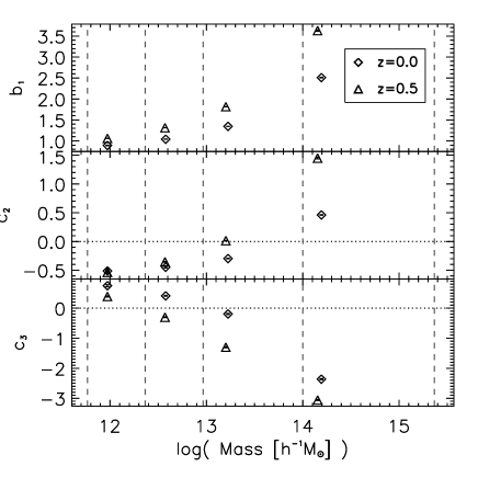
Figure 1: Peak-background split prediction of the bias parameters $b_{1}$, $c_{2}$ and $c_{3}$ for the mass samples M0-M3 versus the mean halo mass of each sample at redshift $z=0.0$ and $z=0.5$ (diamonds and triangles respectively). The mass ranges of the samples are marked by vertical dashed lines.

2.1 Bias predictions

The peak-background split model predicts that the bias parameters in equation (1) are a function of the halo mass (Bardeen et al., 1986; Cole and Kaiser, 1989; Sheth and Tormen, 1999). For deriving these predictions we fit the mass function with the model of Tinker et al. (2010). The low mass sample M1 is thereby excluded from the fitting range, since we expect the mass function measurements to be affected by noise in the halo detection in this mass range (see Hoffmann et al., 2015a, for a detailed discussion). However, this exclusion does not affect the sign of the predicted bias coefficients. The mean bias coefficients of each mass sample, shown in Fig. is then obtained by weighting the bias prediction with the normalised halo mass distribution.

In Fig. 1 we show the predicted mass dependency for bias coefficients up to third order. In Hoffmann et al. (2015a) we compare the predictions for the linear bias parameter with measurements from two-point cross-correlations and find an agreement at the $10$% level. Comparing the second- and third-order bias predictions to measurements from third-order statistics and a direct analysis of matter and halo density fluctuations we find a good qualitative agreement (Bel, Hoffmann, Gaztañaga, in preparation). We shall use these predictions for discussing our results in Section 3.

3 Bias estimators

In this section we study various bias estimators from second- and third-order clustering statistics of haloes and matter, in order to quantify and understand differences between these estimations. Such an understanding is crucial for using third-order statistics in order to break the degeneracy between the linear galaxy (or halo) bias and the linear growth of matter fluctuations, as we discussed in (Hoffmann et al., 2015b).

In this previous study we found that the linear bias from the reduced three-point correlation in configuration space tends to overestimate the linear bias from the two-point correlation, even when the analysis is performed at very large scales ($>30\ h^{-1}$Mpc). Similar findings have been reported in the literature (e.g. Manera and Gaztañaga, 2011). Such deviations can be expected from non-local contributions to the bias function (Chan et al., 2012; Baldauf et al., 2012). Furthermore, non-linear terms in the perturbative expansion of correlations functions, which are usually neglected in the analysis of clustering measurements, can contribute to the deviations between the different bias estimators (Pollack et al., 2012). The goal of this section is to investigate the effect produced on various bias estimators of non-linear (sub-section 3.1) and non-local (sub-sections 3.2 and 3.3) contributions to the biasing function.

Throughout this investigation we shall use the following notations: the density contrast of a stochastic field at position ${\bf r_{i}}$ will be shortly written as $\delta_{y,i}\equiv\delta_{y}({\bf r_{i}})$ where $y$ refers to either haloes ($h$) or matter ($m$). Note that, when no confusion is possible, we will drop the index $i$ referring to the position.

3.1 Bias from second-order statistics

We study second-order statistics of the halo- and matter density fields in terms of the two-point correlation and the variance. The density fields are therefore smoothed with a spherical Top-hat window function of radius $R$. The two-point correlations can be defined as the average products of density contrasts at the positions $\bf{r}_{1}$ and $\bf{r}_{2}$,

$$\xi^{xy}\equiv\langle\delta_{x,1}\delta_{y,2}\rangle(r_{12}),$$ (4)

which is a function of the distance $r_{12}=|\bf r_{2}-\bf r_{1}|$. If the two density contrasts belong to the same density fields (haloes or matter, i.e. $x=y$) equation (4) defines the two-point auto-correlation, denoted in the following as $\xi$ and $\xi_{h}$ for the matter and the halo field respectively. Note that, for a given smoothing window, the variance $\sigma^{2}$ corresponds to the two-point correlation in the limit where $r_{12}=0$. In the case of two different density fields (halo and matter) equation (4) defines the two-point cross-correlation, which we denote as $\xi^{\times}$ in the following.

The average $\langle\ldots\rangle$ refers to all pairs, independently of their orientation. We thereby follow the common assumption of ergodicity such that the ensemble average can be estimated from the mean over the comoving volume in each simulation snapshot. The two-point correlation is therefore an isotropic quantity, in contrast to the three-point correlation, which we study later in Subsection 3.2. Note that we ignore redshift space distortions in this study.

If the biasing relation between matter and haloes was linear ($\delta_{h}=b_{1}\delta_{m}$) then the halo variance $\sigma_{h}^{2}\equiv\langle\delta_{h}^{2}\rangle$, the halo two-point auto-correlation $\xi_{h}\equiv\langle\delta_{h,1}\delta_{h,2}\rangle$, the halo-matter cross-variance $\sigma_{\times}^{2}\equiv\langle\delta_{h}\delta_{m}\rangle$ and the halo-matter two-point cross-correlation $\xi^{\times}\equiv\langle\delta_{h,1}\delta_{m,2}\rangle$, would provide equivalent estimators of the bias parameter $b$. Hence, we can define four linear bias estimators based on second-order statistics as

$$b_{\sigma} \equiv \sigma_{h}/\sigma,$$ (5)

$$b_{\sigma}^{\times} \equiv \sigma_{\times}^{2}/\sigma^{2},$$ (6)

$$b_{\xi} \equiv \sqrt{\xi_{h}/\xi},$$ (7)

$$b_{\xi}^{\times} \equiv \xi^{\times}/\xi.$$ (8)

Any deviation from the equivalence of these estimators provides a way to study the impact of possible non-linear terms in the biasing relation between matter and haloes (e.g. Manera et al., 2010; Saito et al., 2014, respectively). In fact, if the biasing function is a local relation, defined by its Taylor expansion (see equation (1)), one can approximate the auto- and cross-correlation of haloes as a function of one- and two-point statistics of the matter field. Fry and Gaztanaga (1993) and Bel and Marinoni (2012) provide the corresponding expressions respectively for one- and two-point cumulants up to fifth order (i.e. $\langle\delta_{h,1}^{n}\delta_{h,2}^{m}\rangle$ and $n+m\leq 5$), keeping terms up to second order (leading order plus one) in terms of $\xi$ and $\sigma^{2}$.

Since we focus on non-linear effects, we express the second-order statistics of haloes (auto and cross) up to two orders after the leading order, which is keeping only terms of third-order in $\xi$ and $\sigma^{2}$ and lower. In the case of the two-point auto-correlation we obtain

$$\frac{\xi_{h}}{b_{1}^{2}} \simeq \xi+(c_{2}C_{12}+c_{3})\xi\sigma^{2}+\frac{c_{2}^{2}}{2}\xi^{2}$$ (9)

$$+\left(\frac{c_{3}}{3}C_{13}+c_{4}(\frac{C_{12}}{2}+\frac{S_{3}}{3})+\frac{c_{5}}{4}\right.$$

$$\left.+\frac{c_{2}^{2}}{4}C_{22}+\frac{c_{2}}{2}c_{3}C_{12}+\frac{c_{3}^{2}}{4}\right)\xi\sigma^{4}$$

$$+\left(c_{2}c_{3}C_{12}+\frac{c_{2}}{2}c_{4}\right)\xi^{2}\sigma^{2}+\frac{c_{3}^{2}}{6}\xi^{3},$$

while we find for the cross-correlation

$$\frac{\xi^{\times}}{b_{1}} \simeq \xi+\frac{1}{2}(c_{2}C_{12}+c_{3})\xi\sigma^{2}$$ (10)

$$+\frac{1}{2}\left(\frac{c_{3}}{3}C_{13}+c_{4}(\frac{C_{12}}{2}+\frac{S_{3}}{3})+\frac{c_{5}}{4}\right)\xi\sigma^{4},$$

where $C_{nk}$ and $S_{n}$ are respectively the reduced correlators and cumulants of the matter field, defined as $C_{nk}\equiv\langle\delta_{m,1}^{n}\delta_{m,2}^{k}\rangle_{c}/\xi/\sigma^{2(n+k-2)}$ and $S_{n}\equiv\langle\delta_{m}^{n}\rangle_{c}/\sigma^{2(n-1)}$ (see Bernardeau, 1996). The non-linear terms in $\xi$, present in equation (9) and (10), differ from each other. This means that non-linear bias affects the auto- and cross-correlation function of haloes differently. The corresponding expansions for the variance and the cross-variance of haloes can be straightforwardly obtained by taking the one-point limit in the equations (9) and (10) (i.e. $r_{12}=0$). Hence, the reduced correlator $C_{nk}$ corresponds to the reduced cumulant $S_{n+k}$ and the two-point correlation function (auto and cross) converges to the variance (auto and cross). These two expansions show that, at third order in $\sigma^{2}$ and $\xi$, one needs to take into account bias parameters up to fifth order ($c_{5}$). However, since we focus our analysis on scales at which the matter density contrast is small ($\delta_{m}\ll 1$), we will approximate the bias function as a third-order polynomial. In the following, we therefore set the fourth- and fifth-order parameters to zero.

The equations (9) and (10) show that, if only the leading order terms are kept, then the bias estimators (5)-(8) converge to the linear bias $b_{1}$. However, they also tell that, if higher order terms are contributing to the signal, then significant deviations between the estimators must be detectable. In the following, we exploit this fact to test the impact of non-linearities on the estimators (5)-(8).

The auto- and cross-correlation functions are estimated by applying the estimator proposed by Bel and Marinoni (2012) on the halo and the dark matter particle distributions. Its implementation in the MICE-GC simulation is described in Hoffmann et al. (2015b), to estimate the errors we use a Jack-knife method on $64$ cubical cells. For studying the scale dependence we vary the smoothing scale $R$, while we keep the correlation length ratio $r_{12}/R=2$ fixed.

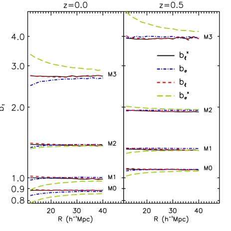
Figure 2: Comparison between four linear bias estimations from measurements of the auto- and cross- variance and the two-point auto- and cross- correlation (blue, green, red and black respectively), derived via equation (5) - (8). Results for the redshifts $z=0.0$ and $z=0.5$ are shown in the left and right panel respectively. The different smoothing scales $R$ of the halo and matter density fields, used for the bias estimations, are shown on the $x$-axis. For measuring $\xi$ and $\xi^{\times}$ we fix $r_{12}=2R$.

The bias measurements for the four mass samples M0-M3 at the redshifts $z=0.0$ and $z=0.5$, derived from the estimators (5)-(8) are presented in Fig. 2. We can see that, on the considered scale range, the estimators involving two-point statistics are in good agreement with each other and display negligible scale dependence. This indicates that higher-order terms in the equations (9) and (10) can indeed be safely neglected. However, estimators involving the variance differ significantly from $b_{\xi}$ and $b_{\xi}^{\times}$, especially at small scales when the matter variance $\sigma^{2}$ approaches unity. Furthermore, they do not mutually agree, even on large scales. Similar results have been obtained by Manera et al. (2010) and Manera and Gaztañaga (2011). In order to explain differences between $b_{\xi}$ and $b_{\xi}^{\times}$ Manera et al. (2010) set $c_{3}=0$ and drop the term in $\sigma^{4}$ into the higher order expansion; although they did not have a theoretical motivation for that.

Following their approach and using the equations (9) and (10) we expand the expressions (5) - (8) up to the second-order in $\sigma^{2}$ and $\xi$ and express $b_{\sigma}$, $b_{\xi}$ and $b_{\sigma}^{\times}$ with respect to $b_{\xi}^{\times}$

$$\left(\frac{b_{\sigma}}{b_{1}}\right)^{2}-\left(\frac{b_{\xi}^{\times}}{b_{1}}\right)^{2}\!\!\! \!\!\!=\!\!\! \!\!\!\left[c_{2}(S_{3}-C_{12})+\frac{c_{2}^{2}}{2}\right]\sigma^{2}$$ (11)

$$\!\!\!+\left[\frac{c_{2}^{2}}{4}(S_{4}-C_{12}^{2})+\frac{c_{3}}{3}(S_{4}-C_{13})\right.$$

$$\!\!\!+\left.\frac{c_{2}c_{3}}{2}(3S_{3}-C_{12})+\frac{c_{3}^{2}}{6}\right]\sigma^{4}$$

$$\left(\frac{b_{\sigma}^{\times}}{b_{1}}\right)^{2}\!\!\!-\left(\frac{b_{\xi}^{\times}}{b_{1}}\right)^{2}\!\!\! \!\!\!=\!\!\! \!\!\!c_{2}(S_{3}-C_{12})\sigma^{2}+\left[\frac{c_{2}^{2}}{4}(S_{3}^{2}-C_{12}^{2})\right.$$ (12)

$$\!\!\!\left.+\frac{c_{3}}{3}(S_{4}-C_{13})\right.$$

$$\!\!\!\left.+\frac{c_{2}c_{3}}{2}(S_{3}-C_{12})\right]\sigma^{4}$$

$$\left(\frac{b_{\xi}}{b_{1}}\right)^{2}\!\!\!-\left(\frac{b_{\xi}^{\times}}{b_{1}}\right)^{2}\!\!\! \!\!\!=\!\!\! \!\!\!\frac{c_{2}^{2}}{2}\xi+\frac{c_{2}^{2}}{4}\left[C_{22}-C_{12}^{2}\right]\sigma^{4}$$ (13)

$$\!\!\!+c_{2}c_{3}C_{12}\xi\sigma^{2}+\frac{c_{3}^{2}}{6}\xi^{2}.$$

With the expressions above one can partially explain the deviations between the different bias estimators, displayed in Fig. 2. We thereby rely on the fact that differences between the linear bias and differences between the second power of these values are monotonically related to each-other, due to the positive amplitude of the linear bias. The first interesting point is to notice that equation (13) does not exhibit any contribution from $\sigma^{2}$ at the leading order. Moreover the contribution from $\sigma^{4}$ vanishes since it has been shown that correlators obey the factorisation rule $C_{nk}=C_{1n}C_{1k}$ (Bernardeau, 1996). As a result equation (13) contains only terms in $\xi$, which is small on the considered scale range ($r_{12}\gtrsim 20h^{-1}$Mpc). This explains the good agreement between $b_{\xi}$ and $b_{\xi}^{\times}$ for all halo mass ranges.

The expression which we obtained for $b_{\xi}$ differs from the one given by Manera et al. (2010) presumably due to a truncation of the higher-order expansion of the halo two-point cross-correlation function by these authors. In addition, our results seem to confirm the necessity they had to set the contribution of order $\sigma^{4}$ and the third-order bias $c_{3}$ to zero in order to explain their results. Note also that at very small scales, Fig. 2 shows that $b_{\xi}$ tends to be larger than $b_{\xi}^{\times}$. This small tendency can be explained by the fact that the leading order term of equation (13) is positive.

Regarding the comparison between $b_{\sigma}^{\times}$ and $b_{\xi}^{\times}$, the leading order term in expression (12) shows that their relative amplitude depends on the sign of $c_{2}$. If it is negative $b_{\sigma}^{\times}$ is lower than $b_{\xi}^{\times}$, which is the case for the mass samples M0-M2 at $z=0$ and M0-M1 at $z=0.5$. The peak-background split bias predictions, displayed in Fig. 1, shows that $c_{2}$ is indeed expected to be negative for these mass samples (see Section 2 for details about the prediction). The deviations between the bias from the variance and the two-point cross-correlation is, at low masses, in good agreement with the one predicted by equation (11). In fact, the leading order term contains two contributions, one in $c_{2}^{2}$ and another in $c_{2}$. The latter being dominant for low masses where $|c_{2}|<1$. It follows that $b_{\sigma}$ is expected to lie between $b_{\sigma}^{\times}$ and $b_{\xi}^{\times}$ which is confirmed by Fig. 2. However, for higher mass bins we observe an opposite tendency to the expected one. By combining equations (11) and (12) one obtains that the relative position between $b_{\sigma}$ and $b_{\sigma}^{\times}$ is

$$\left(\frac{b_{\sigma}}{b_{1}}\right)^{2}\!\!\!-\!\!\!\left(\frac{b_{\sigma}^{\times}}{b_{1}}\right)^{2}\!\!\! \!\!\!=\!\!\! \!\!\!\frac{c_{2}}{2}\sigma^{2}\!\!+\!\!\left[c_{2}c_{3}S_{3}+\frac{c_{2}^{2}}{4}(S_{4}\!\!-\!\!S_{3}^{2})+\frac{c_{3}^{2}}{6}\right]\!\!\sigma^{4}.$$ (14)

As a result when $c_{2}>0$, the bias from the variance is expected to be greater than the bias from the cross-variance. Note also that, even in the particular case of $c_{2}\simeq 0$ (M2 at $z=0.5$), the remaining term in $c_{3}^{2}$ shows that $b_{\sigma}$ must be greater than $b_{\sigma}^{\times}$. The measurements, shown in Fig. 2, exhibit a different behaviour than the one just described. In fact, for the high mass bins M3 at $z=0$ and M2, M3 at $z=0.5$, the estimate from $b_{\sigma}$ stays below the one from $b_{\sigma}^{\times}$. The bias from the variance apparently saturates to the value of the bias from two-point correlations and therefore seems to constitute a more robust linear bias estimator than the cross-variance. Note that, this tendency is observed even at very large scale $R=40\ h^{-1}$Mpc which suggests that non-linear corrections are not responsible.

We conclude that higher-order contributions arising from non-linear bias can only explain partially the relative amplitudes between the linear bias estimators displayed in Fig. 2. This result motivates the introduction of a non-local component in the biasing relation, as suggested in the literature (e.g. Chan et al., 2012; Baldauf et al., 2012; Saito et al., 2014) and also shows that one needs to go beyond second-order statistics. However, we do not expect non-local bias to significantly affect our second-order halo statistics, especially because of the large smoothing scales applied in this analysis. This might not be the case for third-order statistics. We therefore speculated in Hoffmann et al. (2015b) that a non-local component in the biasing relation could explain the differences between second- and third-order bias estimators. In the next subsection, we therefore generalise our analysis in studying linear and quadratics bias estimation from third-order statistics (auto and cross). Finally, we note that the bias estimator based the two-point cross-correlation function ($b_{\xi}^{\times}$) can be considered as a reliable estimator of the linear bias $b_{1}$, we thus consider it as a reference in the following.

3.2 Bias from three-point cross-correlation $b_{Q}^{\times}$

The three-point correlation of the three generic density fields that we label $x$, $y$ and $z$ at the positions ${\bf r_{1}}$, ${\bf r_{2}}$ and ${\bf r_{3}}$ (respectively) is defined as

$$\zeta^{xyz}\equiv\langle\delta_{x,1}\delta_{y,2}\delta_{z,3}\rangle,$$ (15)

where the vectors ${\bf r}_{1}$, ${\bf r}_{2}$ and ${\bf r}_{3}$ form a closed triangle which can be parametrised in terms of the size of its three legs $r_{ij}\equiv|{\bf r_{j}}-{\bf r_{i}}|$ or in terms of the two legs ${\bf r}_{12}$, ${\bf r}_{13}$ and the angle $\alpha_{23}=\text{acos}({\bf\hat{r}}_{12}\cdot{\bf\hat{r}}_{13})$ between them. As for the two-point correlation in Section 3.1 $\langle\ldots\rangle$ denotes the mean over all triangles in the analysed volume. However, in contrast to the two-point correlation, where the average is taken over all pairs of $\delta$ independently of their direction, $\zeta$ is not isotropic as it is sensitive to the shape of the large-scale structure. It therefore provides access to additional information. In case of the auto-correlation the three density contrasts in equation (15) refer to the same density field. The corresponding three-point correlation function of haloes and matter are therefore $\zeta^{hhh}$ and $\zeta^{mmm}$, respectively. To measure the bias from the three-point cross-correlation between haloes and matter densities we compute $\zeta^{hmm}$, $\zeta^{mhm}$, $\zeta^{mmh}$. These quantities are then compared to the hierarchical three-point cross-correlation (Fry, 1984a)

$$\zeta^{hm}_{H}\equiv\xi^{hm}_{12}\xi^{hm}_{13}+\xi^{mh}_{12}\xi^{hm}_{23}+\xi^{mh}_{13}\xi^{mh}_{23}.$$ (16)

Note that here $\xi^{hm}_{ij}$ referrers to the two-point cross-correlation between haloes at position ${\bf r_{i}}$ and matter at position ${\bf r_{j}}$, which is called $\xi^{\times}$ in the remainder of this article. Combining equation (15) and (16) one can define the symmetric reduced three-point cross-correlation function (Pollack et al., 2012)

$$Q_{h}^{\times}\equiv\frac{1}{3}\frac{\zeta^{hmm}+\zeta^{mhm}+\zeta^{mmh}}{\zeta^{hm}_{H}}.$$ (17)

The reduced three-point auto-correlations for matter and halo density fields are defined analogously as $Q_{m}\equiv\zeta^{mmm}/\zeta_{H}^{mm}$ and $Q_{h}\equiv\zeta^{hhh}/\zeta_{H}^{hh}$. This way $Q_{h}^{\times}$, $Q_{h}$ and $Q_{m}$ quantify any departure from the hierarchical ansatz (Fry, 1984b). In the following we will refer to the reduced three-point correlation as the three-point correlation.

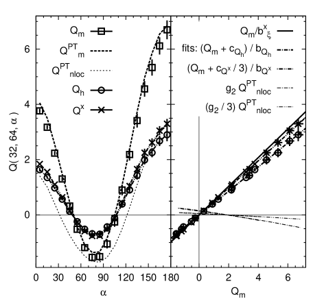
Figure 3: Left: three-point auto- and cross-correlation for matter and haloes ($Q_{h}$, $Q^{\times}$ and $Q_{m}$) in the mass sample M2 at redshift $z=0.5$, measured using triangles with fixed legs of $32$ and $64$ $h^{-1}$Mpc for different opening angles $\alpha$ (circles, crosses and squares respectively). Fits based on the local bias model (i.e. $g_{2}=0$) to $Q_{h}$ and $Q^{\times}$ from equation (18) and (19) are shown as thick dashed-dotted and dash-double dotted lines. Predictions for the matter three-point correlation and the non-local component from perturbation theory ($Q^{PT}_{m}$ and $Q^{PT}_{nloc}$) are shown as thick and thin dashed lines respectively. Right: the $Q_{h}$ and $Q^{\times}$ versus $Q_{m}$ relation, used for deriving the linear and quadratic parameters $b_{1}$ and $c_{2}$ in the local bias model. Thin dashed-dotted and dash-double dotted lines show the non-local contributions to $Q_{h}$ and $Q^{\times}$ respectively, using $g_{2}$ from $\Delta Q_{cg}$, equation (24).

Inserting the non-local quadratic bias model (equation (2)) into the definition of the three-point correlation for haloes yields, via a second-order perturbative expansion, in the limit of small density fluctuations and large triangles

$$Q_{h}=\frac{1}{b_{1}}\bigl{\{}Q_{m}+[c_{2}+g_{2}Q_{nloc}]\bigr{\}},$$ (18)

which can be generalised to the case of three-point cross-correlation,

$$Q_{h}^{\times}=\frac{1}{b_{1}}\bigl{\{}Q_{m}+\frac{1}{3}[c_{2}+g_{2}Q_{nloc}]\bigr{\}}$$ (19)

(see Appendix A). These expressions differ significantly from the ones obtained from the local bias model, as they include the non-local contribution to the three-point halo correlation $Q_{nloc}$, which we present in more detail below. The expression for the local model, which we assumed in Hoffmann et al. (2015b) corresponds to a vanishing non-local bias parameter, i.e. $g_{2}=0$. Since $Q_{nloc}$ is a function of the opening angle $\alpha\equiv\alpha_{23}$, the three-point halo auto- and halo-matter cross-correlations are therefore no longer linearly related to the matter three-point correlation. This $\alpha$ dependence arises from the fact that $Q_{nloc}$ originates from tidal forces, which modify the shape of matter fluctuations.

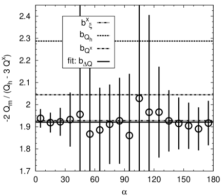
Figure 4: Linear bias of the halo mass sample M2 at the redshift $z=0.5$, measured independently of second-order contributions (local and non-local) to the three-point correlation via equation (23) by combining $Q_{h}$, $Q^{\times}$ and $Q_{m}$ (open circles). The fit to the measurements is shown as solid line. The linear bias measurements, derived from $\xi^{\times}$, $Q_{h}$ and $Q^{\times}$ within the local bias model (via equation (8), (18) and (19) respectively with $g_{2}=0$) are shown as dashed, dash-dotted and dash-double dotted lines respectively.

We can predict $Q_{nloc}$ from the power spectrum, assuming that the perturbations of the density field $\delta_{m}$ are small (i.e. the divergence of the velocity field $\theta_{v}$ in equation (3) is linear and therefore equal to $\delta_{m}$. It also requires to assume that the legs of the considered triangles are large compared to the smoothing radius $R$ (large separation limit, i.e. in equation (3), $W(Rq_{12})\simeq W(Rq_{1})W(Rq_{2})$). For such conditions the perturbation theory (hereafter also referred to as PT) offers the possibility to express the non-local three-point correlation $Q_{nloc}$ in terms of

$$\Gamma_{123}\equiv\left[\xi(r_{12})+3\frac{\phi^{\prime}(r_{12})}{r_{12}}\right]\left[\xi(r_{13})+3\frac{\phi^{\prime}(r_{13})}{r_{13}}\right]L_{2}(\cos\alpha_{12}),$$ (20)

where

$$\phi(r)=\int d^{3}\mathbf{k}\frac{P(k)}{k^{2}}W^{2}(kR)\frac{\sin(kr)}{kr}$$ (21)

and $\phi^{\prime}(r)\equiv\frac{{\mathrm{d}}\phi}{{\mathrm{d}}r}(r)$. One can show that

$$Q_{nloc}(r_{12},r_{13},\alpha)=\frac{2}{3}\left\{\frac{\Gamma_{123}+\Gamma_{312}+\Gamma_{231}}{\zeta^{mm}_{H}}-1\right\}.\\$$ (22)

The angular dependence of the non-local component of the three-point halo auto- and cross-correlation functions is encoded in equation (20) via the second-order Legendre polynomial $L_{2}(\cos\alpha_{12})$. As shown by Barriga and Gaztañaga (2002) in their equation (8), at the tree-level and for large separations, the matter three-point correlation can be expressed in the same way as expression (22). That is with respect to circular permutations of a function $\hat{\Gamma}_{123}$, expressed as a monopole, a dipole and a quadrupole in $\cos(\alpha_{12})$ (similar Legendre expansion have been used in Fourier space by Schmittfull et al., 2015) As a result, a non-local component, such as the tidal field $\mathcal{G}_{2}$ (equation (3)), modifies the amplitude of the quadrupole of $\hat{\Gamma}_{123}$ by an amount proportional to the non-local bias $g_{2}$ (see Appendix A).

Moreover, by comparing equations (18) and (19) one can see that quadratic and non-local contributions to the halo three-point correlation affect the cross-correlations by a factor $1/3$ less than the auto-correlation. The linear bias, in contrast, affects the auto- and cross-correlation equally. We will use this property to isolate the linear from the quadratic and non-local bias, as explained below.

In the following we study non-local contributions to the halo bias in the MICE-GC simulation. Ours measurements of the three-point correlation are based on the algorithm suggested in Barriga and Gaztañaga (2002) (see also Hoffmann et al., 2015b, for studies of numerical effects in this algorithm and the impact of covariance between angular bins on the bias measurements). Errors are derived from $64$ cubical Jack-Knife samples. We first focus on the mass bin M2 at redshift $z=0.5$ to present our methods for extracting the parameters $b_{1}$, $c_{2}$ and $g_{2}$ from three-point correlations, which were computed using triangles with fixed legs of $r_{12}=32$ and $r_{13}=64\ h^{-1}$Mpc. Afterwards we will present results for all mass samples and redshifts at various scales.

3.2.1 Local bias

Our first method for measuring bias from three-point correlations is based on the local bias model ($g_{2}=0$). The linear and quadratic bias parameters are computed from the equations (18) and (19) by fitting the $b_{1}$ and $c_{2}$ parameters which allows for mapping $Q_{m}$ into $Q_{h}$ and $Q_{h}^{\times}$, i.e. $Q_{h}=(Q_{m}+c_{2})/b_{1}$ and $Q_{h}^{\times}=(Q_{m}+\frac{c_{2}}{3})/b_{1}$. The fitting procedure is explained in Hoffmann et al. (2015b). The two estimations of the doublet $b_{1}$ and $c_{2}$ are respectively called $b_{Q}$, $c_{Q}$ and $b_{Q}{{}^{\times}}$, $c_{Q}^{\times}$. In Fig. 3 we show how well a linear relation, expected from the local bias model, describes the mapping between the matter three-point correlation and the three-point auto- and cross-correlation functions of haloes. However, we can see that the slope of the linear relation is different when considering auto- and cross-correlations, which indicates that the two methods deliver inconsistent results (see right panel of Fig. 3) . As explained in Chan et al. (2012) this linear relation between matter and haloes might arise from a projection effect due to the fact that we neglect the non-local component $g_{2}Q_{nloc}$. In Fig. 3 we show that, if the contribution of $Q_{nloc}$ is small compared to $Q_{m}$ (i.e. $g_{2}$ is small, see Fig. 8), then they can indeed be approximately related by a linear relation. The ignored non-local contribution to halo three-point correlations can therefore be absorbed by $b_{1}$ and $c_{2}$, without substantially decreasing the goodness of the $Q_{h}$ and $Q^{\times}$ fits. The same effect has been shown in Fourier space by Baldauf et al. (2012) in their Fig. 1. This ignorance might lead to incorrect bias measurements, unless $g_{2}=0$.

3.2.2 Non-local bias

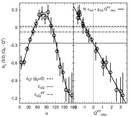
Figure 5: Left: The difference between the three-point auto- and cross-correlation $Q_{h}$ and $Q^{\times}$ ($\Delta Q_{cg}$), multiplied with the linear bias from the two-point correlation (open circles) as a function of triangle opening angle $\alpha$ for M2 at $z=0.5$. According to equation (24) this expression is equivalent to $c_{2}+g_{2}Q_{nloc}$. If the bias function is quadratic and local, the measurements should correspond to the quadratic bias parameter $c_{2}$, as measured from the halo-matter cross-correlation via equation (19) with $g_{2}=0$ (dash-dotted line). Fits from equation (24), based on the PT prediction for the non-local component, $Q_{nloc}$, are shown as thick solid line. The quadratic bias parameter, derived from this fit ($\Delta Q_{cg}$) is shown as dashed line. The corresponding effective quadratic bias parameter (equation (37)) is shown as dashed-double dotted line. The three-point correlations were calculated from triangles with fixed leg of $r_{12}=r_{13}/2=32\ h^{-1}$Mpc. Right: same as left panel, but showing the measurements versus the $Q_{nloc}$ prediction for each opening angle.

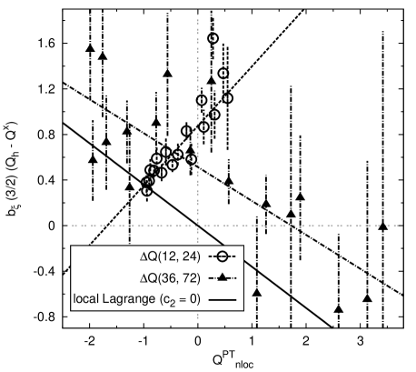
Figure 6: Same as right panel of Fig. 5, but for the halo mass sample M3 at the redshift $z=0.0$. Results are shown for triangles with fixed legs $r_{12}=r_{13}/2$ of $12$ and $36\ h^{-1}$Mpc (open circles and filled triangles respectively). Dashed and dashed-dotted lines are the corresponding fits to equation (24), used to derive the quadratic and non-local bias $c_{2}$ and $g_{2}$. The black solid line corresponds to the local Lagrangian prediction for $c_{2}+g_{2}Q_{nloc}$ with $c_{2}=0$ and $g_{2}=2\gamma_{2}/b_{1}$, while $\gamma_{2}=-(2/7)(b_{1}-1)$. The $\gamma_{2}$ values from these fits are shown in Fig. 8.

Our second method for measuring bias from three-point correlations is a new a approach, which combines auto- and cross-correlations. These two statistics can be combined in two different ways which allow us to isolate the linear bias from quadratic and non-local contributions to the bias model. Both combinations take advantage of the fact that the linear bias, $b_{1}$, affects $Q_{h}$ and $Q_{h}^{\times}$ equally, which is not the case for the quadratic and non-local contributions, $c_{2}$ and $g_{2}$. The linear bias can be obtained by combining the equations (18) and (19),

$$b_{\Delta Q}\equiv-2\frac{Q_{m}}{\Delta Q},$$ (23)

where $\Delta Q\equiv Q_{h}-3Q_{h}^{\times}$. The interesting property of this linear bias estimator is that it is independent from quadratic (local and non-local) contributions to the bias function. It can therefore be used to verify if such contributions are indeed the reason for deviations between linear bias estimations from two- and three-point correlations, as we speculated in Hoffmann et al. (2015b). Note that the relevant quantities involved in equation (23) depend on the opening angle $\alpha$, so does the estimator $b_{\Delta Q}$. Hence, our final $b_{\Delta Q}$ measurement is derived by fitting a constant to $b_{\Delta Q}(\alpha)$. The use of $\Delta Q$ has also the advantage that off-diagonal elements in the covariance matrix between different opening angles are smaller. This covariance is difficult to access and its Jack-Knife estimation can affect the bias estimation at the $5$% level (Hoffmann et al., 2015b).

We show $b_{\Delta Q}$ for M2 at $z=0.5$ in Fig. 4 at each angle probed by the three-point functions together with the corresponding fit. In the same figure we also display the estimations for the linear bias, derived from three-point auto- and cross-correlations ($b_{Q}$ and $b_{Q^{\times}}$, obtained from equations (18) and (19), assuming the local bias model, i.e. $g_{2}=0$). As a reference, we also include the linear bias measurements from the two-point cross-correlation, $b_{\xi}^{\times}$, which we consider to be a reliable estimate of the true linear bias (see Section 3.1). The comparison in Fig. 4 reveals that the measurement and the fit of the hybrid bias estimator $b_{\Delta Q}$ are consistent with the reference $b_{\xi}$, while we see that the biases obtained from $b_{Q}$ and $b_{Q^{\times}}$ are over estimating the linear bias. This result confirms our speculation in Hoffmann et al. (2015b), that differences between $b_{\xi}$ and $b_{Q}$ are mainly due to a non-local term in the bias model. Furthermore we verified that also the magnitude of the overestimation is in agreement with what we expect from neglecting non-local contributions. However, as we pointed out in this aforementioned study, linear bias measurements from three-point correlations can also be affected by numerical effects, originating from the algorithm employed for deriving $Q$ as well as shortcomings in the estimation of the $Q$ covariance between different angular bins.

One can notice that, as expected in case of non-local bias, the overestimation is larger in case of the auto-estimator ($b_{Q}$) compared to the cross-estimator ($b_{Q^{\times}}$). Note that Pollack et al. (2012) found an opposite trend, analysing a different simulation in Fourier space with a different mass resolution and cosmology. Their linear bias measurements from the bispectrum are closer to peak-background split predictions than measurements from three-point cross-correlations, while the predictions might be lower than the true linear bias (see e.g. Hoffmann et al., 2015a).

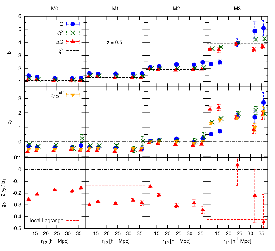
Figure 7: Scale dependence of bias measurements from three-point correlations. Measurements were derived using triangles with $r_{13}/r_{12}=2$ configuration, while scale of the smaller triangle leg, $r_{12}$, is denoted on the x-axis (slightly shifted for clarity). Results are shown for the four mass samples M0-M3 (from left to right) at redshift $z=0.5$. The linear and quadratic bias (top and central panel respectively), obtained from three-point auto- and cross-correlations using the local bias model ($g_{2}=0$) via the equations (18) and (19) are shown as blue circles and green crosses respectively. The linear, quadratic and non-local bias, measured using combinations of three-point auto- and cross-correlations ($\Delta Q$, equation (23 ) and (24)) are shown as red triangles. The linear bias is compared with reference measurements from the two-point cross-correlation ($b_{\xi}^{\times}$), shown as black, dashed line. The quadratic bias measurements are compared with effective quadratic bias (equation (37)), shown as orange triangles. The non-local bias parameter $g_{2}\equiv 2\gamma_{2}/b_{1}$ (bottom panel) is compared with predictions from the local Lagrangian model ($\gamma_{2}=-(2/7)(b_{1}-1)$). (red dashed line). Error bars denote $1\sigma$ uncertainties.

3.2.3 Linear and quadratic terms

In order to further verify the presence of non-local contributions to the bias function we separate $Q_{nloc}$ from $Q_{m}$ by subtracting $Q_{h}^{\times}$ from $Q_{h}$ and define

$$\Delta Q_{cg}\equiv Q_{h}-Q_{h}^{\times}=\frac{2}{3}\frac{1}{b_{1}}\left[c_{\Delta Q}+g_{\Delta Q}Q_{nloc}\right],$$ (24)

where $c_{\Delta Q}$ and $g_{\Delta Q}$ are the estimators of $c_{2}$ and $g_{2}$ in equations (18) and (19). If the bias function is quadratic in $\delta_{m}$ and local then the non-local bias parameter $g_{2}$ is zero. Hence,

$$c_{\Delta Q}=b_{1}\Delta Q_{cg}(3/2)$$ (25)

should correspond to $c_{2}$, independently of the opening angle $\alpha$. In the left panel of Fig. 5, we show $c_{\Delta Q}$, together with $c_{2}$, estimated from $Q_{h}$ and $Q^{\times}$ ($c_{Q}$ and $c_{Q^{\times}}$ respectively) from the local bias model (equations (18) and (19), for $g_{2}=0$). In the same figure we also show $c_{2}$ derived from fitting ${\Delta Q_{cg}}$ taking into account a possible non-local bias $g_{2}$. The first important point is that the measured $c_{\Delta Q}$ shows a very clear angular dependence, with a maximum at around $80$ degrees and a positive curvature. The local quadratic model therefore clearly fails in describing the impact of bias on three-point correlations.

The right panel of Fig. 5 displays the measurements of $\Delta Q_{cg}$ with respect to the tidal, non-local component of the three-point function $Q_{nloc}$, as predicted by equation (22). It shows that measurements are compatible with a linear relation between $\Delta Q_{cg}$ and $Q_{nloc}$, which is expected in the second order non-local bias model. It therefore confirms the presence of non-local bias due to tidal forces ($\mathcal{G}_{2}$) in the matter field. For such a linear relation, the value of $\Delta Q_{cg}$ corresponds to the second-order bias $c_{\Delta Q}$ when $Q_{nloc}=0$, while its slope provides a direct insight to the non-local bias $g_{2}$. Finally, by comparing the various estimates of the second-order local bias $c_{2}$, one can see that, when assuming a local bias, the results differ significantly from the ones obtained when taking into account a possible non-local component into the biasing relation. However, the estimation of $c_{\Delta_{Q}}$ and $g_{2}$ might be affected by shortcomings of the PT predictions for $Q_{nloc}$.

To verify how well the PT predictions describe the measurements at different scales we show the relation between $\Delta Q_{cg}$ and $Q_{nloc}$ derived from triangles with fixed legs $r_{12}=r_{13}/2$ of $12$ and $36\ h^{-1}$ Mpc respectively in Fig. 6 for the mass samples M3 at $z=0.0$, for which we find a large non-local bias amplitude. At large scales ($r_{12}=36\ h^{-1}$ Mpc) the slope of the measured $\Delta Q_{cg}$ - $Q_{nloc}$ relation is comparable with the local Lagrangian prediction. Interestingly at small scales the $\Delta Q_{cg}$ - $Q_{nloc}$ relation is also linear, while the slope has the opposite sign than at large scales. The linearity at small scales indicates that higher-order terms enter the $Q$ in a similar way as second-order non-local contributions to the bias function. This suggests that linear bias measurements can be improved by using the prediction for $Q_{nloc}$, while using the local Lagrangian prediction for the non-local bias $g_{2}$ is only appropriate at extremely large scales.

3.2.4 Scale dependence

Based on the methods for measuring linear, second-order and non-local bias from $Q$ and $Q^{\times}$ ($b_{Q}$, $b_{Q^{\times}}$, $b_{\Delta Q}$, $c_{Q}$, $c_{Q^{\times}}$ and $c_{\Delta Q}$), which were presented above, we now apply our analysis to each of the mass samples M0-M3 at $z=0.5$. We study the scale dependence of our results as before by varying the size of the triangle leg $r_{12}$ between $12\ h^{-1}$Mpc and $36\ h^{-1}$Mpc) while fixing $r_{12}/r_{13}=1/2$. The various bias estimations are presented in Fig. 7 for different triangles sizes, defined by the length of $r_{12}$.

From the comparison between the different bias estimations we draw similar conclusions as from the example of M2 at $z=0.5$. On linear scales (sufficiently large triangles) the linear bias parameters obtained from each method reaches a regime in which they become scale independent. However, they do not converge to the same value. In case of the linear bias, only $b_{\Delta Q}$ is in agreement with $b_{\xi}^{\times}$, while $b_{Q}$ and $b_{Q^{\times}}$ overestimate the linear bias; this overestimation is stronger in the case of $Q$ than $Q^{\times}$.

The scale dependence shown for the high mass bin M3 in Fig. 7 shows that, if the analysis is performed at too small scales, then one can measure a positive non-local bias, while it is in reality negative (as we see from the results derived at large scales). We indeed verified that for highly biased tracers and small triangles, the curvature of $c_{\Delta Q}$ flips from positive to negative. This scale dependence indicates a domination of the signal by non-linear terms in these cases. However, for lower mass samples and large scales, for which we expect non-linear contributions to converge to zero, we still see a strong angular dependence of $c_{\Delta Q}$, which speaks for the presence of non-local bias contributions. Hence, we have shown that all the mass sample used in the present analysis exhibit a detectable non-local component.

In case of estimators of the second-order bias $c_{2}$ (middle panel of Fig. 7) we observe the same tendency, however we do not have a reference estimate. As a result we shall be more confident in the estimation of $c_{2}$ coming from $c_{\Delta Q}$. We compare the latter to measurements from third-order moments in Section 4. A comparison with $c_{2}$ derived from various methods will be presented in Bel et al. (in preparation).

The bottom panel shows that each mass sample comprises non-local bias which significantly differs from the local model $\gamma_{2}=0$. These measurements therefore constitute the first detection of non-local bias in configuration space. In the case of M0 and M1 the amplitude of the non-local bias strongly differs from the local Lagrangian biasing relation between the halo and matter field (Mo and White, 1996).

3.2.5 Non-local to linear bias relation

Figure 8: Non-local bias parameters $\gamma_{2}$ and $g_{2}=2\gamma_{2}/b_{1}$ versus the linear bias from the two-point cross-correlation, $b^{\times}_{\xi}$. Measurements, derived from $\Delta Q_{cg}=(Q_{h}-Q^{\times})$ via equation (24) are shown as symbols with $1\sigma$ errors. Results are shown for $Q$ measurements based on triangles with fixed legs of $r_{12}=12$, $24$ and $36\ h^{-1}$Mpc and $r_{12}=r_{13}/2$ configurations (from the top to the bottom). Crosses, open squares, open circles and open triangles show the non-local bias, measured for the mass samples M0, M1, M2 and M3 respectively at redshift $z=0.0$. Stars, closed squares, closed circles and closed triangles show the corresponding M0-M3 measurements at $z=0.5$. The measurements for $r_{12}=36\ h^{-1}$Mpc are approximated with $\gamma_{2}=-(2/7)(b_{1}-0.8)$ (black dash-dotted lines) and compared with the local Lagrangian prediction ($\gamma_{2}=-(2/7)(b_{1}-1)$) as well as to a fit given by Chan et al. (2012, $\gamma_{2}=-(2/7)(b_{1}-1.43)$), shown as solid and dashed black lines respectively.

Following Chan et al. (2012), we compare our non-local bias measurements to the linear bias derived from the two-point cross-correlation in the top panels of Fig. 8. This comparison includes measurements at redshift $0.0$ and $0.5$ which are based on triangles with $r_{12}/r_{13}=1/2$ configurations. For very large triangles ($r_{12}=36\ h^{-1}$Mpc) our results indicate a linear relation between the non-local $\gamma_{2}$ and the linear $b_{1}$ bias, as expected for the local Lagrangian biasing. However, the amplitude of this relation lies below the local Lagrangian prediction, which is the opposite of what was reported by Chan et al. (2012). Some work is currently ongoing, aiming to explain whether these differences result from the fact that Chan et al. (2012) conduct their measurements using the Bispectrum in Fourier space, while we employ the reduced three-point correlation in configuration space. A further contribution to the discrepancies could arise from differences in the simulation, such as mass resolution effects, or differences between cosmological parameters.

As a matter of fact, our measured $b_{1}-\gamma_{2}$ relation shows the same tendency as those of Sheth et al. (2013), Baldauf et al. (2012) and Saito et al. (2014) who also find (in Fourier space) $\gamma_{2}$ to be below the local Lagrangian prediction. The simulations employed in the two latter studies are based on cosmologies similar to MICE-GC, while Chan et al. (2012) study a simulation with a initial power spectrum which is significantly different in terms of its normalisation $\sigma_{8}(z=0.0)$ and spectral index $n_{s}$. Note also that the departures from the local Lagrangian prediction in Fig. 7 are strongly scale dependent for highly biased samples ($b_{\xi}\gtrsim 2$), which indicates the presence of non-linear contamination to $Q_{m}$ and $Q_{nloc}$ (e.g. Saito et al., 2014).

3.3 Bias from third-order moments $b_{\tau}^{\times}$

An alternative approach for exploring the higher-order statistical properties of the large-scale structure are one- and two-point third-order statistics, respectively referred to as skewness and reduced correlator. They can be understood as the one- and two-point limits of the reduced three-point correlation (e.g. Gaztanaga and Frieman, 1994). Since these statistics are isotropic, they do not provide access to the full third-order hierarchy probed by the three-point correlation (i.e. the shape of the large-scale structure). However, this section will show that this apparent disadvantage leads to a cancellation of non-local bias which is useful for linear bias measurements, as we discuss later.

The auto-skewness and the reduced auto-correlator of the matter density fluctuations $\delta_{m}$ are respectively defined as

$$S_{3}\equiv\frac{\langle\delta_{m}^{3}\rangle}{\sigma^{4}},$$ (26)

and

$$C_{12}(r)\equiv\frac{\langle\delta_{m,1}\delta_{m,2}^{2}\rangle}{\sigma^{2}\xi(r)}$$ (27)

(see Goroff et al., 1986; Bernardeau, 1996). As in the previous subsection $\sigma$ and $\xi$ refer to the matter field. The auto-skewness and the reduced auto-correlator for halo density fluctuations, $\delta_{h}$, are defined analogously to equation (26) and (27). The skewness is directly related to the asymmetry of the one-point probability distribution of $\delta_{m}$, while the correlator tells how the quadratic field is correlated with itself on a given scale $r$. Their properties have been extensively investigated in literature (e.g. Bernardeau, 1996; Gaztañaga et al., 2002; Bel and Marinoni, 2012). As for the two-point and three-point correlation we also study the cross-skewness $S_{3,h}^{\times}$ and the cross-correlator $C_{12,h}^{\times}$ in order to investigate the impact of non-linearities, non-local bias as well as shot-noise on the measurements. We define these quantities as

$$S_{3,h}^{\times}\equiv\frac{\langle\delta_{h}\delta_{m}^{2}\rangle}{\sigma_{\times}^{4}}$$ (28)

and

$$C_{12,h}^{\times}\equiv\frac{\langle\delta_{h,1}\delta_{h,2}\delta_{m,2}\rangle}{\sigma_{\times}^{2}\xi_{h}}.$$ (29)

As in previous sub-sections the indices $h$ and $m$ refer, respectively, to the halo and matter density contrast.

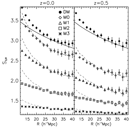
Figure 9: Left: reduced cross Skewness $S_{3}^{\times}$, measured at the two redshifts $z=0.0$ and $z=0.5$ for matter (filled circles), and the four halo mass samples M0-M3 (diamonds, triangles, squares and stars respectively). Right: corresponding measurements for the reduced cross-correlator $C_{12}$. On each panel we display the tree-level PT predictions for $S_{3}$, equation (27) in Hoffmann et al. (2015b). For $C_{12}$ we show two predictions. The dotted line displays the one from equation (28) in Hoffmann et al. (2015b) and the solid black line shows the one taking into account the small separation contribution (Bel in preparation). We also display in grey dashed lines the fits to $S_{3}^{\times}$ and $C_{12}^{\times}$ from the equations (35) and (36).

For measuring the auto skewness $S_{3}$ and the auto correlator $C_{12}$ we follow Bel and Marinoni (2012) by setting up a regular grid of spherical cells of radius $R$ and counting the number of objects (haloes or dark matter particles) per cell. After assigning a number density contrast $\delta_{N}$ to each grid cell we derive the auto-skewness $S_{3}$ as

$$S_{3,N}=\frac{\langle\delta_{N}^{3}\rangle-3\langle\delta_{N}^{2}\rangle\bar{N}^{-1}+2\bar{N}^{-2}}{(\langle\delta_{N}^{2}\rangle-\bar{N}^{-1})^{2}}.$$ (30)

In order to estimate the reduced correlator $C_{12}$, we consider the density contrast $\delta_{N,1}\equiv\delta_{N}$ for each grid cell. We then place an isotropic distribution of cells at distance $r$ around the central cell and assign the number density contrast $\delta_{N,2}$ to each of these surrounding cells. By averaging over all grid points in the simulation volume we estimate the correlator as

$$C_{12,N}=\frac{\langle\delta_{N,1}\delta_{N,2}^{2}\rangle-2\langle\delta_{N,1}\delta_{N,2}\rangle\bar{N}^{-1}}{\langle\delta_{N,1}\delta_{N,2}\rangle(\langle\delta_{N}^{2}\rangle-\bar{N}^{-1})},$$ (31)

where $\bar{N}$ is the average number of halo or dark-matter particles per cell in the simulation box. These estimators are corrected for shot-noise, assuming the local Poisson process approximation (Layzer, 1956). Note that, in order to be able to handle the large number of dark matter particles, we use only $1/700$ of the total number of particles in the dark matter simulation output. In principle this neglection of particles introduces additional shot-noise errors but we have tested that it does not affect the measurements.

Following the same method, the cross-skewness $S_{3,h}^{\times}$ is estimated as

$$S_{3,h}^{\times}=\frac{\langle\delta_{N,h}\delta_{N}^{2}\rangle-\langle\delta_{N,h}\delta_{N}\rangle\bar{N}^{-1}}{(\langle\delta_{N,h}\delta_{N}\rangle^{2}},$$ (32)

where the sub-index $h$ again refers to halo density field. Note that we correct the cross-skewness differently for shot-noise than the auto-skewness, since the former depends on the matter-field at the power of $2$. Finally, since the cross-correlator does not involve any powers of the same density field larger than unity, the reduced cross-correlator $C_{12,h}^{\times}$ is expected to be insensitive to Poisson shot-noise. Hence we estimate it directly from equation (29). The corresponding errors are estimated with Jack-Knife sampling, using $64$ cubical cells.

Our measurements of the skewness and the reduced correlator are presented as a function of smoothing scale $R$ in Fig. 9 for the redshifts $z=0.0$ and $z=0.5$. As in Section 3.1 the scale dependence is explored by varying the smoothing scale $R$ while we fix the ratio $r/R=2$ in case of the correlator. In the same figure we also show the PT predictions for the dark matter field. The skewness of the dark matter field appears to be redshift independent in the linear regime ($R\gtrsim 20h^{-1}$Mpc), which is in good agreement with the tree-level PT prediction (Bernardeau, 1992). At smaller smoothing scales the redshift dependence becomes more significant which has been shown by Fosalba and Gaztanaga (1998) to be due to non-linear loop corrections. The reduced correlator of the dark matter field shows only a weak redshift dependence, even for small smoothing radii ($R\lesssim 10h^{-1}$Mpc). In Hoffmann et al. (2015b) we have shown that the measured matter correlator is in disagreement with the tree-level PT prediction (dotted blue line in the right panel of Fig. 9). We argued that this is due to the fact that the standard tree-level prediction (Bernardeau, 1996; Bel and Marinoni, 2012) neglects the small separation contributions. We are indeed looking at the correlation between adjacent spheres. In the right panel of Fig. 9 we display also the tree-level prediction (magenta dotted line) which takes into account the small separation contribution (Bel in preparation) arising from the mode-coupling induced by the smoothing process. The observed agreement confirms that for small separations it is mandatory to take into account the smoothing in a proper way.

In Fig. 9 we also show for the first time measurements of the halo-matter cross-skewness and cross-correlator. Comparing these measurements to our results for the auto-skewness and the auto-correlator, presented in Hoffmann et al. (2015b), we notice two qualitative differences. The first difference is that the cross-skewness for the highest mass sample M3 increases at small scales, while we found an opposite trend only for M3 in case of the auto-skewness. The latter measurement should be more affected by shot-noise than the corresponding cross-skewness one or than measurements at lower mass samples; this is due to the low number density of M3 haloes. Furthermore the impact of shot-noise increases at small scales, where the cell volumes are small as well. The decrease of the M3 auto-skewness at small scales might therefore be attributed to a failure of Poisson shot-noise correction, indicating the presence of non-Poisson shot noise for highly biased samples.

The second difference is that the amplitudes of the cross-skewness and the cross-correlator increase monotonically with the halo mass. We did not find such a monotonic behaviour for the auto-skewness and the auto-correlator in Hoffmann et al. (2015b) which has been also confirmed by Angulo et al. (2008). This difference can be explained by the fact that the bias parameters affect the auto- and cross-statistics differently, as we demonstrate in the following.

3.3.1 Bias relations

The skewness and the correlator of the matter field can be related to the corresponding halo and halo-matter cross-statistics via the non-local bias model. In analogy to the three-point correlation, one can express, at the leading order, the cross-statistics between haloes and matter as function of the bias parameters by inserting the bias functions from equation (2) into the definitions (26) - (29). In order to take into account the non-local component, we further assume that perturbations are well described by tree-level PT. It leads to the following expressions for the skewness, correlator, cross-skewness and cross-correlator of haloes

$$S_{3,h} \simeq \left[S_{3}+3(c_{2}-\frac{2}{3}g_{2})\right]/b_{1}$$ (33)

$$C_{12,h} \simeq \left[C_{12}+2(c_{2}-\frac{2}{3}g_{2})\right]/b_{1}$$ (34)

$$S_{3,h}^{\times} \simeq \left[S_{3}+c_{2}-\frac{2}{3}g_{2}\right]/b_{1}$$ (35)

$$C_{12,h}^{\times} \simeq \left[C_{12}+c_{2}-\frac{2}{3}g_{2}\right]/b_{1}$$ (36)

(see Appendix A). On can notice the similarity with the corresponding equations for the three-point auto- and cross-correlations (18) and (19). The contribution of the second-order biases (local or non-local) to the cross-skewness and cross-correlators is three times smaller than in case of the auto-skewness and two time smaller than in the auto-correlator.

In contrasts to the three-point correlations the second-order non-local contributions, described by equation (3), can be taken into account as an effective second-order local bias,

$$c_{2}^{\mathrm{eff}}=c_{2}-\frac{2}{3}g_{2},$$ (37)

which consists of a local ($c_{2}$) and a non-local ($g_{2}$) contribution. This absorption of non-local contributions by $c_{2}^{\mathrm{eff}}$ results from the isotropy of spherically averaged quantities, such as the skewness or the correlator (Chan et al., 2012, already presented this effective local description of non-local biasing for spherically symmetric matter perturbations). Hence, we do not expect the estimation of the linear bias via the equations (33)-(36) to be significantly affected by non-local contributions to the bias model. However, such non-local contributions will modify systematically the estimation of the quadratic bias parameter $c_{2}$. We will discuss the impact on the bias estimations in Section 4.

By varying the bias parameters in equation (35) and (36) we can fit the measurements of the auto-skewness and auto-correlator for matter to the measured halo-matter cross-skewness and cross-correlator. We see in Fig. 9 that these fits are in reasonable agreement with the measurements for $R\gtrsim 20\ h^{-1}$Mpc. At smaller scales the fits lie typically above the measurements. This latter discrepancy is lower than in the case of the auto-statistics, presented in Hoffmann et al. (2015b). We therefore conclude that non-linearities and non-local contributions have less impact on the third-order cross-statistics than on the corresponding auto-statistics.

In order to measure the linear and the quadratic bias parameters we combine equations (35) and (36) in a way which allows us to measure linear and quadratic contributions (local or non-local) to the bias model independently from each other

$$b_{\tau}^{\times}\!\!\! \equiv \!\!\frac{{\displaystyle\,S_{{3}}-\,C_{{12}}}}{{\displaystyle\,S_{{3,h}}^{\times}-\,C_{{12,h}}^{\times}}}\equiv\frac{\tau^{\times}}{\tau_{h}^{\times}}$$ (38)

$$c_{\tau}^{\times}\!\!\! \equiv \!\!\frac{{\displaystyle S_{{3}}C_{{12,h}}^{\times}-C_{{12}}S_{{3,h}}^{\times}}}{{\displaystyle\tau_{h}^{\times}}}.$$ (39)

This type of $S_{3}$ and $C_{12}$ combinations has been suggested for the auto-skewness and the auto-correlators by Szapudi (1998) and Bel and Marinoni (2012) and was further studied by Hoffmann et al. (2015b).

3.3.2 Bias measurements

Our measurements for the bias parameters, obtained from equations (38) and (39), are displayed in Fig. 10 with respect to the smoothing radius $R$. As for the measurements of $C_{12}$ we set the distance between two spherical grid cells with radius $R$ to $r=2R$. The measurements were performed for the four mass bins M0-M3 at redshift $0.0$ and $0.5$. We compare our results with corresponding measurements from the auto-skewness and the auto-correlator, $b_{\tau}$ and $c_{\tau}$, presented in Hoffmann et al. (2015b).

Figure 10: Top: Linear bias obtained from the $b_{\tau}$ and $b_{\tau}^{\times}$ estimators (respectively open and filled diamonds) compared to the reference linear bias from the two-point cross-correlation (dashed line) with respect to the smoothing scales $R$ and at $z=0.5$ for the mass samples M0-M3 (Table 1). Bottom: Quadratic reduced bias parameter $c_{2}$ estimated with $c_{\tau}$ estimator (diamonds) at $z=0.5$. Error bars denote $1-\sigma$ uncertainties.

The upper panel shows the linear bias measurements together with the reference measurements from the two-point cross-correlation (equation (8)), which we consider to be a robust estimate of the true linear bias (see Section 3.1). We find that, for all masses, $b_{\tau}^{\times}$ is less sensitive than $b_{\tau}$ to the considered scale. This finding is consistent with our previous conclusion from Fig. 9 that cross-statistics must be less affected by non linearities. The scale dependence is stronger for higher masses which can be attributed to non-linear and non-local terms in the bias functions (Saito et al., 2014). This interpretation is supported by the fact that we find a better agreement between $b_{\xi}$ and $b_{\tau}$ at redshift $0.5$ than at redshift $0.0$.

Our second-order bias estimations $c_{\tau}$ and $c_{\tau}^{\times}$ are shown in the bottom panel of Fig. 10. It is worth noticing that, as opposed to linear bias estimators, the $c_{\tau}^{\times}$ estimator is affected by a larger scatter in the measurement than $c_{\tau}$. This can be explained by lower sensitivity of the cross-statistics ($S^{\times}_{3,h}$ and $C^{\times}_{12,h}$) to non-linear and non-local contributions to the bias functions (i.e. $c_{2}^{\mathrm{eff}}$), compared the auto-statistics ($S_{3,h}$ and $C_{12,h}$). This is indeed related to their monotonic behaviour with respect to the considered mass sample (see Fig. 9); the main dependence comes from the linear bias. The combination of $S^{\times}_{3,h}$ and $C^{\times}_{12,h}$ to obtain $c_{\tau}^{\times}$ therefore provides weak and noisy constrains on $c_{2}^{\mathrm{eff}}$.

The fact that for highly biased tracers (M3) any non-local component in the bias relation is unable to explain why the two estimators $b_{\tau}$ and $b_{\tau}^{\times}$ do not converge to the $b_{\xi}^{\times}$ estimator indicates the presence of a velocity bias, which has been shown to appear for very massive haloes (see Chan et al., 2012). This kind of contribution would add a dipole to the biasing relation which could modify significantly the $b_{\tau}$ and $b_{\tau}^{\times}$ estimators.

4 Results

In the previous section we studied measurements of the linear, quadratic and non-local bias parameters ($b_{1}$, $c_{2}$ and $g_{2}$ respectively). These measurements were derived from three different methods which are all based on third-order statistics of halo- and matter density fluctuations.

Two of these methods employ three-point auto-and cross-correlations. The first method is to compare the three-point cross-correlation with the three-point matter auto-correlation to derive the linear and quadratic bias parameters via equation (19). This approach is based on the assumption of a local bias model. The linear and quadratic bias parameters, derived from this method are called $b_{Q}^{\times}$ and $c_{Q}^{\times}$ respectively. The second method is to use particular combinations of three-point auto- and cross-correlations. The linear bias parameters, derived this way via equation (23), $b_{\Delta Q}$, are independent of any quadratic contributions (local or non-local) to the bias function, as explained in the previous section. The quadratic and non-local bias parameters are obtained simultaneously by fitting predictions for the non-local component of the three-point correlation function, $Q^{PT}_{nloc}$, to $\Delta Q_{cg}$, defined in equation (24). The quadratic parameters from such measurements is called $c_{\Delta Q}$.

The third method is to use a combination of the halo-matter cross-correlator and cross-skewness with the corresponding auto-statistics for the matter field. The linear bias, derived from this so-called $\tau^{\times}$ estimator via equation (38) is called $b^{\times}_{\tau}$. The effective quadratic bias parameter, obtained from equation (39) is called $c^{\times}_{\tau}$. We demonstrated in the previous section that this effective quadratic bias ($c_{2}^{\mathrm{eff}}$) consists of the quadratic bias and a non-local contribution, which cannot be distinguished from each other with the $\tau$ method (see equation 37). This feature is a consequence of the isotropy of the skewness and the correlator. Since we have shown that cross-statistics are weakly sensitive to the effective second order bias and therefore more sensitive to shot-noise we will use instead the $c_{\tau}$ estimator. For clarity, in Table 2 we summarize our estimators and the notations that we use.

Table 2: Bias estimators, definitions and notations

Symbol	Definition	Equation
$b_{\xi}^{\times}$	$\xi^{\times}/\xi$	Eq.(8)
$b_{Q}$	$Q_{h}=\frac{1}{b_{Q}}\bigl{\{}Q_{m}+c_{Q}\bigr{\}}$	Eq.(18)
$b_{Q}^{\times}$	$Q_{h}^{\times}=\frac{1}{b_{Q}}\bigl{\{}Q_{m}+\frac{c_{Q}}{3}\bigr{\}}$	Eq.(19)
$b_{\Delta Q}$	$b_{\Delta Q}\equiv-2\frac{Q_{m}}{Q_{h}-3Q_{h}^{\times}}$	Eq.(23)
$b_{\tau}$	$\frac{\tau}{\tau_{h}}$	Hoffmann et al. (2015b)
$b_{\tau}^{\times}$	$\frac{\tau^{\times}}{\tau_{h}^{\times}}$	Eq.(38)
$c_{Q}$	$Q_{h}=\frac{1}{b_{Q}}\bigl{\{}Q_{m}+c_{Q}\bigr{\}}$	Eq.(18)
$c_{Q}^{\times}$	$Q_{h}^{\times}=\frac{1}{b_{Q}}\bigl{\{}Q_{m}+\frac{c_{Q}}{3}\bigr{\}}$	Eq.(19)
$c_{\Delta Q}$	$c_{\Delta Q}=b_{1}\frac{3}{2}[Q_{h}-Q_{h}^{\times}]$	Eq.(25 )
$c_{\tau}$	$\frac{{S_{{3}}C_{{12,h}}-C_{{12}}S_{{3,h}}}}{{\displaystyle\tau_{h}}}$	Hoffmann et al. (2015b)
$c_{\tau}^{\times}$	$\frac{{S_{{3}}C_{{12,h}}^{\times}-C_{{12}}S_{{3,h}}^{\times}}}{{\displaystyle\tau_{h}^{\times}}}$	Eq.(39)

In this section, we aim at comparing the bias estimations coming from these three methods. We therefore present the different linear and quadratic bias estimations for the four mass samples M0-M3 at the redshifts $0.0$ and $0.5$ versus the mean halo mass in each sample in Fig. 11. Our bias measurements based on thee-point correlations are done using triangles with $r_{12}=r_{13}/2=36\ h^{-1}$Mpc. The $\tau^{\times}$ estimations are based on fits of $b^{\times}_{\tau}$ and $c^{\times}_{\tau}$ between $26\leq R\leq 40\ h^{-1}$Mpc using $r_{12}=2R$ configurations.

The linear bias estimations from the different methods are presented in the upper panel of Fig. 11. We compare these estimations to reference measurements from the two-point cross-correlation, defined in equation (8), which we consider as reliable (see Section 3.1). The relative deviations to this reference linear bias are shown in the central panel.

We find that the estimator $b_{Q}^{\times}$, which neglects the non-local bias, overestimates the linear bias by $5$-$10$%. The fact that we found a stronger overestimation for $b_{Q}$ ($10$-$30$%) in Hoffmann et al. (2015b) can be attributed to the lower impact of non-local contributions to the three-point cross-correlation compared to the corresponding auto-correlation, as discussed in the previous section.

The linear bias parameters from $\Delta Q$ is in excellent agreement with the reference for all mass ranges and at both redshifts. Deviations are in the range of the $1\sigma$ of $b_{\Delta Q}$, while the latter roughly correspond to $1$% of the amplitude. For the mass sample M3 deviations become slightly larger and more significant. We find this agreement also for smaller triangle scales, as we demonstrated for $z=0.5$ in Fig. 7 and discussed in the previous section.

Our linear bias measurements from the $\tau_{\times}$ estimator differs by less than $5$% from the reference linear bias for the mass samples M0-M2 at both redshifts. Such deviation are comparable with the $1\sigma$ errors and are therefore not significant. At the highest mass sample M3 the linear bias derived from $\tau^{\times}$ deviates significantly from the reference. We found a similar behaviour in Hoffmann et al. (2015b) for the $\tau$ estimator. If this deviation was due to exclusion effect (leading to a wrong shot noise correction) then we would expect the $b_{\tau}^{\times}$ estimator to be only weakly affected, which is not the case. An alternative explanation for these strong deviations can be the presence of velocity bias, which possibly cannot be neglected in this mass regime as we argued in Section 3.3.

Figure 11: Top: Summary of the linear bias measurements presented in this work. Results are shown for the redshifts $z=0.0$ and $z=0.5$ (left and right respectively) versus the mean halo mass of each mass sample M0-M3, defined in Table 1 (lower and upper limits of the mass samples are marked by vertical grey dashed lines. Symbols are slightly shifted along the the mass axis for clarity). The smaller panel shows the relative deviation of each estimator with respect to the linear bias from the two-point cross-correlation ($b_{\xi}^{\times}$, solid lines). The estimators $b_{Q}^{\times}$, $b_{\Delta Q}$ and $b_{\tau}^{\times}$ (from equations (19), (23) and (38) respectively) are displayed respectively by open circles, open triangles and open squares. For measuring $b_{Q}^{\times}$ we assumed a local bias model, i.e. $g_{2}=0$. Bottom: Summary of the second-order bias measurements $c_{Q}^{\times}$, $c_{\Delta Q}$ and $c_{\tau}$ from the same bias estimation methods, as used for the linear bias in the top panel (equation (19)), (24) and (39) respectively). The $c_{2}^{\mathrm{eff}}$ (equation (37)), obtained by combining $c_{2}$ and $g_{2}$ from the $\Delta Q$ method, is represented with filled triangles. For estimations based on $Q$ we used triangles with $(r_{12},r_{13})=(36,72)\ h^{-1}$Mpc configurations. Estimations using the $\tau$ method are fits between $26\leq R\leq 40\ h^{-1}$Mpc. Error bars denote $1\sigma$ uncertainties.

The lower panel of Fig. 11 shows how the methods compare in terms of estimating the second-order bias parameter $c_{2}$. Moreover, given that $c_{\tau}$ only estimates the effective second-order bias we also show the $c_{2}^{\mathrm{eff}}$ (green triangles) computed from $c_{2}$ and $g_{2}$ (equation (37)) given by the $\Delta Q$ method. At redshift $z=0.0$ we can see that the contribution of the non-local bias to the $c_{2}^{\mathrm{eff}}$ is very small which, given the error on the $c_{2}^{\mathrm{eff}}$ measured from $c_{\tau}$, does not allow to separate the two measurements. At least, we see that for low mass bins the two effective second-order bias values agree within the errors. Hence, we can conclude that at redshift $z=0.0$ the effective second-order bias is a good approximation of the second-order bias. Regarding low mass bins at redshift $z=0.5$ one can see that, even if the effective $c_{2}$ from $\Delta Q$ differs significantly from $c_{2}$, it is difficult to say which one is in better agreement with $c_{\tau}$. The latter seems to be in better agreement with $c_{2}$ than the expected $c_{2}^{\mathrm{eff}}$ coming from the three-point correlations. In case of the high mass bin, we observe again at both redshifts that the $c_{\tau}$ estimator delivers unreasonable results. We conclude that the $c_{\tau}$ estimator can be used to estimate the second-order local bias parameter as long as the considered tracer are not too massive ($\gtrsim 10^{14}h^{-1}M_{\odot}$). Finally, we can say that the second-order bias, estimated from the three-point cross-correlation when the non-local bias is neglected leads to significant departure from the one obtained from $\Delta Q_{cg}$.

5 Summary and Conclusion

We studied linear, quadratic and, for the first time in configuration space, non-local bias of halo clustering with respect to the clustering of the dark matter field. We therefore employed various second- and third-order statistics of halo and matter density fluctuations in the MICE-GC simulation. Our goal was to find if the overestimation of the linear bias parameter by the three-point auto-correlation, which we found previously in Hoffmann et al. (2015b) (see also Manera and Gaztañaga, 2011; Pollack et al., 2012), can be attributed to shortcomings of the local quadratic bias model. Understanding this difference is crucial for breaking the degeneracy between growth and bias with three-point correlations, which would strongly amplify the statistical power of large-scale structure surveys. To achieve this goal we employ auto- and cross-statistics to disentangle the effects of linear bias on second- and third-order halo statistics from those originating from non-linear and non-local bias.

We started our analysis verifying how well the second-order clustering of haloes can be described by a linear bias model in Section 3.1. Comparing the amplitudes of the variances $\sigma$ to those of two-point correlations $\xi$ we found the former to be significantly affected by non-linear and possibly non-local contributions to the bias function. However, the halo two-point correlations are well described by a linear local bias model down to scales of $10\ h^{-1}$Mpc. For this reason we employed such measurements from the two-point cross-correlation as an estimator for the linear bias, used as reference in the subsequent analysis. Note that we also expect departures from scale independent bias (see Desjacques et al., 2010) for highly biased samples at scales close the BAO peak ($\gtrsim 80\ h^{-1}$Mpc, Hoffmann et al., 2015a, b), while the large errors at such scales should prevent a strong impact of this effect.

For studying the impact of non-linear and non-local bias on the three-point correlation we compared in Section 3.2 bias measurements from the (reduced) three-point halo-matter cross-correlation to those from the auto-correlation from our previous study, using the local quadratic model. We found the linear bias from the cross-correlation to be closer to the reference than the linear bias from the auto-correlation. This is expected from second-order perturbation theory, which predicts the three-point cross-correlation to be less affected by quadratic local and non-local bias than the corresponding auto-correlation (compare equation (18) and (19)). However, the three-point cross-correlations delivers, as the corresponding auto-correlation, linear bias measurements, which lie significantly above the reference from the two-point correlation.

To further verify if this overestimation can be attributed to non-linear and non-local contributions to the bias model we take advantage of the fact that three-point auto- and cross-correlations are affected differently by non-linear and non-local bias, but equally by the linear bias (see again equation (18) and (19)). This property allows for combinations of the auto- and cross-statistics which isolate the linear from the non-linear and the non-local bias. We find the linear bias, measured by such a combination of three-point correlations independently of quadratic or non-local bias (equation 23) to be in excellent agreement with the reference from the two-point correlation (Fig. 4). This finding is a strong indication that non-local terms are indeed the reason for the overestimation of linear bias from three-point correlation, when ignoring them by assuming a local quadratic bias model. This approach could be used to measure linear bias by cross-correlating galaxy with lensing maps. The presence of non-local bias also becomes apparent in our measurements of non-linear bias contributions (local and non-local) via equation (24), which are in good agreement with predictions for the non-local contributions to the three-point correlation (Fig. 5). Our results therefore constitute the first detection of non-local bias in configuration space and demonstrate the paramount importance of taking it into account when analysing galaxy surveys.

When the considered scales are two small ($r_{12}\lesssim 30\ h^{-1}$Mpc), the non-local bias parameter $\gamma_{2}$, derived from our measurements, shows a strong scale-dependence, indicating the presence of higher-order local or non-local terms in the bias function. Instead, for scales larger than $36\ h^{-1}$Mpc we find a linear relation between the non-local and the linear bias, over the whole mass range, as predicted by the local Lagrangian bias model (Fig. 8). However, the amplitude of this relation lies significantly below the local Lagrangian prediction. This is in agreement with results from Baldauf et al. (2012) and Saito et al. (2014), but in contradiction with results from Chan et al. (2012), who find the non-local bias to be above the local Lagrangian prediction. Whether this latter disagreement comes from the fact that Chan et al. (2012) analysed the bispectrum in Fourier space using different simulations is the subject of current investigations. An alternative reason for this discrepancy could be the inaccuracy of the prediction of the non-local contribution to the three-point correlation of matter, from which we derive the non-local bias parameter.

Besides three-point correlations we studied in Section 3.3 bias from one- and two-point third-order statistics (i.e. the skewness and the reduced correlator respectively). These two statistics can be combined into the so-called $\tau$-estimator (Bel and Marinoni, 2012), which allows us to measure the linear and quadratic bias parameters (the latter being local and non-local) independently from each other. An important difference to the three-point correlation is that the $\tau$-estimator is an isotropic quantity. Non-local contributions to the bias function are therefore absorbed in an effective quadratic bias parameter (equation (37)). Hence, the quadratic and non-local bias cannot be distinguished from each other by the $\tau$-estimator. Our measurements show that the $\tau$ method delivers a linear bias estimation which agrees at the $1\sigma$ level with the reference linear bias from the two-point correlation at scales larger than $20h^{-1}$Mpc, while the errors on the bias correspond to $\simeq 5$% of the amplitude (Fig. 10).

This result lines up with our findings from the combination of three-point auto- and cross correlations in the sense that third-order statistics is able to deliver accurate estimations of the linear bias when the employed estimator is independent of non-local and possible higher-order contributions to the bias function.

Interestingly the linear as well as the quadratic bias estimations derived from the $\tau$ method are failing when measurements are performed in samples of very massive haloes ($M\gtrsim 10^{14}$M_⊙). Since this effect appears in both, the auto- and the cross-statistics it might be attributed to velocity bias, rather than non-Poissonian shot-noise as we speculated in Hoffmann et al. (2015b); further investigations are needed to understand this effect.

Summarising our various bias estimations in Fig. 7, we find an overall variation in the linear bias of $\sim 10$% with respect to the reference from the two-point cross-correlation. Deviations from the reference are more significant for measurements from the three-point correlation, which are based on the quadratic local bias model. The bias estimators, which are independent from non-local contributions ($\Delta Q$ and $\tau$) do not differ significantly from the reference for the linear bias, except for $\tau$ in the high mass range, as we saw previously.

Comparing the quadratic bias from the different estimators we found the effective $c_{2}$, obtained from the $\tau$-estimator, to be close to $c_{2}$ measured with the combination of three-point auto- and cross-correlations, which takes into account non-local bias. This finding shows that one can reasonably neglect the non-local bias contribution when using the $\tau$-estimator to measure the quadratic bias parameter. This neglection is not possible for three-point correlations, as those deliver quadratic bias parameters which are significantly higher than measurements, which take non-local bias into account.

Our results show that the local quadratic bias model is inadequate to describe halo bias in the MICE-GC simulation. Non-local second-order terms need to be taken into account for accurate measurements of the linear bias with three-point correlation function. Two approaches are possible to do so. Non-local bias can be isolated from linear bias by combining different third-order statistics (i.e. $\tau$ or $\Delta Q$), or the non-local contributions need to be directly modelled. The first approach, on which we focused in this analysis, might be implemented in terms of cross-correlations between lensing and galaxy maps. We will test the second approach in a future analysis, but already provide here an expression for the non-local contribution to the three-point correlation in configuration space. At scales below $30h^{-1}$Mpc we find indications for the presence of higher-order terms in the bias function (local or non-local). Modelling the non-local bias as a linear function of the linear bias parameter, as suggested by the local Lagrangian bias model, therefore appears to be only suitable at very large scales.

In a future work (Bel, Hoffmann, Gaztañaga, in preparation) we plan to compare the linear and second-order bias measurement, obtained in the present analysis to peak-background split predictions from Hoffmann et al. (2015a) and also bias parameters obtained by directly comparing halo- and matter over densities in the MICE-GC simulation. These various bias estimations can be used to verify the universal relation between linear and non-linear bias parameters, which we presented in Hoffmann et al. (2015a).

Appendix A Non-local bias: a perturbative approach

In this section, the Fourier transform $f({\bf q})$ or $f({\bf k})$ of a configuration space quantity $f({\bf x})$ or $f({\bf r})$ is defined as $f({\bf q})\equiv(2\pi)^{-3}\int f({\bf x})e^{-i{\bf x}\cdot{\bf q}}d^{3}{\bf x}$.

We assume that for large smoothing scales matter perturbations are small such that they are well described by perturbation theory. We further assume that on such scales, the biasing function is described by the equation (2) of this paper, which is

$$\delta_{h}({\bf x})=b_{1}\left\{\delta_{m}({\bf x})+\frac{c_{2}}{2}(\delta_{m}^{2}({\bf x})-\langle\delta_{m}^{2}\rangle)+\frac{\gamma_{2}}{b_{1}}\mathcal{G}_{2}({\bf x})\right\},$$ (40)

where

$$\mathcal{G}_{2}({\bf x})=-\int\beta_{12}\theta_{v}({\bf q}_{1})\theta_{v}({\bf q}_{2})\hat{W}[q_{12}R]e^{i{\bf q}_{12}\cdot{\bf x}}d^{3}{\bf q}_{1}d^{3}{\bf q}_{2}$$

and $\beta_{12}\equiv 1-\left(\frac{{\bf q}_{1}\cdot{\bf q}_{2}}{q_{1}q_{2}}\right)^{2}$, hence $\langle\mathcal{G}_{2}\rangle=0$. The velocity field ${\bf v}$ is normalised in such a way that at linear order its divergence is given by the Poisson equation $-\theta_{v}^{(1)}=\delta_{m}^{(1)}\equiv\delta_{L}$. In the present calculation and in all this paper we work with density fields which are convolved with a Top-hat window function of typical size $R$. In addition, we assume that perturbations are small and can therefore be described at second order by

$$\delta_{m}({\bf x})=\delta_{L}({\bf x})+\delta_{m}^{(2)}({\bf x}),$$ (41)

where $\delta_{L}({\bf x})$ is the linear contribution to the fluctuations. And the second-order contribution (see Bernardeau et al., 2002) can be expressed as

$$\delta_{m}^{(2)}=\int F_{2}({\bf q}_{1},{\bf q}_{2})\delta_{L}({\bf q}_{1})\delta_{L}({\bf q}_{2})\hat{W}[q_{12}R]e^{i{\bf q}_{12}\cdot{\bf x}}d^{3}{\bf q}_{1}d^{3}{\bf q}_{2},$$ (42)

where the second-order perturbation theory kernel is defined as $F_{2}({\bf q}_{1},{\bf q}_{2})\equiv 1+\frac{1}{2}\frac{{\bf q_{1}}{\bf q_{2}}}{q_{1}q_{2}}\left(\frac{q_{2}}{q_{1}}+\frac{q_{1}}{q_{2}}\right)-g\beta_{12}$. This kernel shows that at second order, non-linearities arise due to mode-coupling. The factor $g$ is the second-order growth factor which reduces to $2/7$ in an Einstein-de Sitter universe or as long as the growth rate of structures is given by $f=[\Omega_{m}(z)]^{1/2}$. This function of time, can be identified with the function $B$ in Catelan et al. (1995), or it is related to the function $\kappa$ ($\kappa+g=1/2$) introduced by Bouchet et al. (1992), and is aslo related to the $\mu$ function ($\mu+2g=1$) defined in Kamionkowski and Buchalter (1999).

In the following, in order to use lighter notations we define $\nu\equiv\delta_{h}/b_{1}$. Using equation (40) and expansion (41) we can express $\nu$ at second order as

$$\nu=\delta_{L}+\frac{c_{2}}{2}\left[\delta_{L}^{2}-\langle\delta_{L}^{2}\rangle\right]+\nu^{(2)},$$ (43)

where the quantity $\nu^{(2)}$ is arising from an effective mode coupling kernel such that

$$\nu^{(2)}\equiv\int F_{2}^{\mathrm{eff}}({\bf q}_{1},{\bf q}_{2})\delta_{L}({\bf q}_{1})\delta_{L}({\bf q}_{2})\hat{W}[q_{12}R]e^{i{\bf q}_{12}\cdot{\bf x}}d^{3}{\bf q}_{1}d^{3}{\bf q}_{2}.$$ (44)

Note that the effective second-order kernel $F_{2}^{\mathrm{eff}}$ is obtained by substituting $g$ by $g+\gamma_{2}/b_{1}$ in $F_{2}$. From equation (43), taken at three positions $\bf r_{1}$, $\bf r_{2}$ and $\bf r_{3}$, we can express the three-point correlation function of $\nu$, $\zeta^{\nu}\equiv\langle\nu({\bf x_{1}})\nu({\bf x_{2}})\nu({\bf x_{3}})\rangle$ we obtain

$$\zeta^{\nu} = \zeta^{L}+\frac{c_{2}}{2}\left[\langle\delta_{L}^{2}({\bf r_{1}})\delta_{L}({\bf r_{2}})\delta_{L}({\bf r_{3}})\rangle+perm\right]$$ (45)

$$-\frac{c_{2}}{2}\left[\xi^{L}_{23}\langle\delta_{L}^{2}\rangle+perm\right]$$

$$+\langle\nu^{(2)}({\bf r_{1}})\delta_{L}({\bf r_{2}})\delta_{L}({\bf r_{3}})\rangle+perm,$$

where use the definitions $\xi^{L}_{ij}\equiv\langle\delta_{L}({\bf r_{i}})\delta_{L}({\bf r_{j}})\rangle$ and $\zeta^{L}\equiv\langle\delta_{L}({\bf x_{1}})\delta_{L}({\bf x_{2}})\delta_{L}({\bf x_{3}})\rangle$ . Assuming that the linear part of the density field $\delta_{L}$ is Gaussian, then its three-point correlation function is null and its four-point expectation value can be expressed as (Fry, 1984b)

$$\langle\delta_{L}({\bf r_{1}})\delta_{L}({\bf r_{2}})\delta_{L}({\bf r_{3}})\delta_{L}({\bf r_{4}})\rangle=\xi^{L}_{12}\xi^{L}_{34}+\xi^{L}_{13}\xi^{L}_{24}+\xi^{L}_{14}\xi^{L}_{23}$$

from which we can derive (${\bf r_{1}}={\bf r_{4}}$) that $\langle\delta_{L}^{2}({\bf r_{1}})\delta_{L}({\bf r_{2}})\delta_{L}({\bf r_{3}})\rangle=\xi_{23}^{L}\langle\delta_{L}^{2}\rangle+2\xi^{L}_{12}\xi^{L}_{13}$. The first term cancels with the third term of equation (45). As a result we obtain that

$$\zeta^{\nu}=c_{2}\left[\xi^{L}_{12}\xi^{L}_{13}+perm\right]+\mathcal{J}_{123}+perm,$$ (46)

where $\mathcal{J}_{123}\equiv\langle\nu^{(2)}({\bf r_{1}})\delta_{L}({\bf r_{2}})\delta_{L}({\bf r_{3}})\rangle$. This expression has been calculated by Bel (in preparation) who has shown that taking into account the convolution with the spherical Top-hat filter is very well approximated by a Legendre expansion at second order (which turns out to be exact when no smoothing is applied). Hence

$$\mathcal{J}_{123} \simeq 2(1-2g/3)\xi^{L}_{12}\xi^{L}_{13}+A_{R}(r_{12},r_{13})$$ (47)

$$+B_{R}(r_{12},r_{13})L_{1}(\mu_{23})$$

$$+\left[C_{R}(r_{12},r_{13})+4gD_{R}(r_{12},r_{13})\right]L_{2}(\mu_{23}),$$

where $A_{R}$, $B_{R}$, and $C_{R}$ and $D_{R}$ are obtained from integrals over the linear power spectrum and $\mu_{ij}\equiv\cos\alpha_{ij}$. In practice Bel (in preparation) has shown that in the large separation limit these functions can be identified with the functions $\xi(r_{12})$ ($\xi_{12}^{L}$ in our notations) and $\phi(r_{12})$ introduced by Barriga and Gaztañaga (2002). It reads,

$$A_{R}(r_{12},r_{13}) \simeq 0$$ (48)

$$B_{R}(r_{12},r_{13}) \simeq -\left[{\xi_{12}^{L}}^{\prime}\phi^{\prime}(r_{13})+{\xi_{13}^{L}}^{\prime}\phi^{\prime}(r_{12})\right]$$ (49)

$$C_{R}(r_{12},r_{13}) \simeq 0$$ (50)

$$D_{R}(r_{12},r_{13}) \simeq \frac{1}{3}\left[\xi^{L}_{12}+3\frac{\phi^{\prime}(r_{12})}{r_{12}}\right]\left[\xi_{13}^{L}+3\frac{\phi^{\prime}(r_{13})}{r_{13}}\right],$$ (51)

where $\phi(r)\equiv\int{\mathrm{d}}^{3}\mathbf{k}\frac{P(k)}{k^{2}}W^{2}(kR)\frac{\sin(kr)}{kr}$ and ${}^{\prime}\equiv\frac{{\mathrm{d}}}{{\mathrm{d}}r}$.

In addition, since we saw that $g\rightarrow g+\gamma_{1}/b_{1}$ by substituting it in equation (47) one can split $\mathcal{J}_{123}$ in two contributions

$$\mathcal{J}_{123}=\hat{\Gamma}_{123}+g_{2}\mathcal{K}_{123},$$ (52)

where $\mathcal{K}_{123}\equiv\frac{2}{3}\left[\Gamma_{123}-\xi_{12}\xi_{13}\right]$ is the non-local part which has been introduced in equation (20) and $\hat{\Gamma}_{123}$ can be expressed as

$$\hat{\Gamma}_{123} = 2(1-2g/3)\xi^{L}_{12}\xi^{L}_{13}+A_{R}(r_{12},r_{13})$$ (53)

$$+B_{R}(r_{12},r_{13})L_{1}(\mu_{23})$$

$$+\left[C_{R}(r_{12},r_{13})+4/3gD_{R}(r_{12},r_{13})\right]L_{2}(\mu_{23}).$$

From equation (53), we can express the three-point correlation function of the matter field as

$$Q_{m}^{PT}=\frac{\hat{\Gamma}_{123}+\hat{\Gamma}_{231}+\hat{\Gamma}_{312}}{\zeta_{H}^{m}},$$ (54)

which is equivalent to the expression given in Barriga and Gaztañaga (2002). By analogy, we can define a non-local three-point function $Q_{nloc}$ as

$$Q_{nloc}\equiv\frac{\mathcal{K}_{123}+\mathcal{K}_{231}+\mathcal{K}_{312}}{\zeta_{H}^{m}}.$$ (55)

The definition (55) can be written in terms of the function $\Gamma_{123}$ and its permutations

$$Q_{nloc}=\frac{2}{3}\left\{\frac{\Gamma_{123}+\Gamma_{231}+\Gamma_{312}}{\zeta_{H}^{L}}-1\right\},$$ (56)

where $\Gamma_{123}=D_{R}(r_{12},r_{13})L_{2}(\mu_{23})$ which contains only a quadrupole contribution. On the other hand, from equation (45), we can express the reduced three-point function of haloes $Q_{h}=b_{1}^{-1}\zeta^{\nu}/\zeta_{H}^{L}$ with respect to $\hat{\Gamma}_{123}$ and $\mathcal{K}_{123}$

$$b_{1}Q_{h}=c_{2}+\frac{\hat{\Gamma}_{123}+perm}{\zeta_{H}^{L}}+g_{2}\frac{\mathcal{K}_{123}+perm}{\zeta_{H}^{L}}.$$ (57)

Finally, using definitions introduced before, we find that the reduced three-point function of haloes can be expressed as

$$Q_{h}=b_{1}^{-1}\left\{Q_{m}+c_{2}+g_{2}Q_{nloc}\right\}.$$ (58)

In the end, from equation (58) we can take the limiting cases which correspond to the skewness and the correlator. In case of the skewness Bel (in preparation) has shown that only the monopole contributes. As a result $\Gamma_{123}$ and all its permutations are null therefore

$$S_{3,h}=b_{1}^{-1}\left\{S_{3}+3(c_{2}-\frac{2}{3}g_{2})\right\}.$$ (59)

The second limiting case is obtained when $r_{12}=r_{13}$ and $\alpha_{23}=0$, in this case the permutations $\Gamma_{231}$ and $\Gamma_{312}$ are null so only the $\Gamma_{123}$ is contributing. As a result we get

$$C_{12,h}=b_{1}^{-1}\left\{C_{12}+2[c_{2}-\frac{2}{3}g_{2}+2g_{2}/3D_{R}(r_{12},r_{12})]\right\},$$ (60)

however the function $D_{R}(r_{12},r_{12})$ contributes by less than $5$%/$2$% on scales greater/below than $R=20h^{-1}Mpc$ compared to $C_{12}$. As a result considering that this term is multiplied by $2/3g_{2}$ it will contribute in total at most to $2$% (high mass bin) and to less than $0.1$% for lower mass bins and can be therefore safely neglected, it reads

$$C_{12,h}=b_{1}^{-1}\left\{C_{12}+2(c_{2}-\frac{2}{3}g_{2})\right\}.$$ (61)

The same kind of approach can be used to generalize the relations 58, 59 and 61 to their corresponding cross-statistics. Note that those relations are valid at the three-level and do not imply the large separation limit approximation.

References

- Angulo et al. (2008) Angulo R.E., Baugh C.M., Lacey C.G., 2008, MNRAS, 387, 921
- Baldauf et al. (2012) Baldauf T., Seljak U., Desjacques V., McDonald P., 2012, Phys.Rev.D, 86, 083540
- Bardeen et al. (1986) Bardeen J.M., Bond J.R., Kaiser N., Szalay A.S., 1986, ApJ, 304, 15
- Barriga and Gaztañaga (2002) Barriga J., Gaztañaga E., 2002, MNRAS, 333, 443
- Bel and Marinoni (2012) Bel J., Marinoni C., 2012, MNRAS, 424, 971
- Bernardeau (1992) Bernardeau F., 1992, ApJ, 392, 1
- Bernardeau (1996) Bernardeau F., 1996, A&A, 312, 11
- Bernardeau et al. (2002) Bernardeau F., Colombi S., Gaztañaga E., Scoccimarro R., 2002, Phys. Rept., 367, 1
- Bouchet et al. (1992) Bouchet F.R., Juszkiewicz R., Colombi S., Pellat R., 1992, ApJL, 394, L5
- Buchalter and Kamionkowski (1999) Buchalter A., Kamionkowski M., 1999, ApJ, 521, 1
- Cabré and Gaztañaga (2009) Cabré A., Gaztañaga E., 2009, MNRAS, 393, 1183
- Catelan et al. (1995) Catelan P., Lucchin F., Matarrese S., Moscardini L., 1995, MNRAS, 276, 39
- Chan et al. (2012) Chan K.C., Scoccimarro R., Sheth R.K., 2012, Phys.Rev.D, 85, 083509
- Cole and Kaiser (1989) Cole S., Kaiser N., 1989, MNRAS, 237, 1127
- Crocce et al. (2013) Crocce M., Castander F.J., Gaztanaga E., Fosalba P., Carretero J., 2013, ArXiv e-prints
- Davis et al. (1985) Davis M., Efstathiou G., Frenk C.S., White S.D.M., 1985, ApJ, 292, 371
- de la Torre et al. (2013) de la Torre S., et al., 2013, A&A, 557, A54
- Desjacques et al. (2010) Desjacques V., Crocce M., Scoccimarro R., Sheth R.K., 2010, Phys.Rev.D, 82, 103529
- Eriksen and Gaztañaga (2015) Eriksen M., Gaztañaga E., 2015, ArXiv e-prints
- Fosalba and Gaztanaga (1998) Fosalba P., Gaztanaga E., 1998, MNRAS, 301, 503
- Fosalba et al. (2015a) Fosalba P., Crocce M., Gaztañaga E., Castander F.J., 2015a, MNRAS, 448, 2987
- Fosalba et al. (2015b) Fosalba P., Gaztañaga E., Castander F.J., Crocce M., 2015b, MNRAS, 447, 1319
- Fry (1984a) Fry J.N., 1984a, ApJL, 277, L5
- Fry (1984b) Fry J.N., 1984b, ApJ, 279, 499
- Fry and Gaztanaga (1993) Fry J.N., Gaztanaga E., 1993, ApJ, 413, 447
- Gaztañaga and Lobo (2001) Gaztañaga E., Lobo J.A., 2001, ApJ, 548, 47
- Gaztañaga et al. (2002) Gaztañaga E., Fosalba P., Croft R.A.C., 2002, MNRAS, 331, 13
- Gaztanaga and Frieman (1994) Gaztanaga E., Frieman J.A., 1994, ApJL, 437, L13
- Goroff et al. (1986) Goroff M.H., Grinstein B., Rey S.J., Wise M.B., 1986, ApJ, 311, 6
- Hoffmann et al. (2015a) Hoffmann K., Bel J., Gaztañaga E., 2015a, MNRAS, 450, 1674
- Hoffmann et al. (2015b) Hoffmann K., Bel J., Gaztañaga E., Crocce M., Fosalba P., Castander F.J., 2015b, MNRAS, 447, 1724
- Kamionkowski and Buchalter (1999) Kamionkowski M., Buchalter A., 1999, ApJ, 514, 7
- Layzer (1956) Layzer D., 1956, AJ, 61, 383
- Lue et al. (2004) Lue A., Scoccimarro R., Starkman G., 2004, Phys.Rev.D, 69, 044005
- Manera and Gaztañaga (2011) Manera M., Gaztañaga E., 2011, MNRAS, 415, 383
- Manera et al. (2010) Manera M., Sheth R.K., Scoccimarro R., 2010, MNRAS, 402, 589
- Marín (2011) Marín F., 2011, ApJ, 737, 97
- Marín et al. (2013) Marín F.A., et al., 2013, MNRAS, 432, 2654
- Mo and White (1996) Mo H.J., White S.D.M., 1996, MNRAS, 282, 347
- Piazza et al. (2014) Piazza F., Steigerwald H., Marinoni C., 2014, Journal of Cosmology and Astroparticle Physics, 5, 043
- Pollack et al. (2012) Pollack J.E., Smith R.E., Porciani C., 2012, MNRAS, 420, 3469
- Reid et al. (2012) Reid B.A., et al., 2012, MNRAS, 426, 2719
- Ross et al. (2007) Ross N.P., et al., 2007, MNRAS, 381, 573
- Saito et al. (2014) Saito S., Baldauf T., Vlah Z., Seljak U., Okumura T., McDonald P., 2014, Phys.Rev.D, 90, 123522
- Samushia et al. (2012) Samushia L., Percival W.J., Raccanelli A., 2012, MNRAS, 420, 2102
- Schmittfull et al. (2015) Schmittfull M., Baldauf T., Seljak U., 2015, Phys.Rev.D, 91, 043530
- Sheth and Tormen (1999) Sheth R.K., Tormen G., 1999, MNRAS, 308, 119
- Sheth et al. (2013) Sheth R.K., Chan K.C., Scoccimarro R., 2013, Phys.Rev.D, 87, 083002
- Song and Percival (2009) Song Y.S., Percival W.J., 2009, Journal of Cosmology and Astroparticle Physics, 10, 004
- Springel (2005) Springel V., 2005, MNRAS, 364, 1105
- Steigerwald et al. (2014) Steigerwald H., Bel J., Marinoni C., 2014, ArXiv e-prints
- Szapudi (1998) Szapudi I., 1998, MNRAS, 300, L35
- Tinker et al. (2010) Tinker J.L., Robertson B.E., Kravtsov A.V., Klypin A., Warren M.S., Yepes G., Gottlöber S., 2010, ApJ, 724, 878
- Wu et al. (2010) Wu H.Y., Zentner A.R., Wechsler R.H., 2010, ApJ, 713, 856