A Singular Value Decomposition-based Factorization and Parsimonious Component Model of Demographic Quantities Correlated by Age
Predicting Complete Demographic Age Schedules with Few Parameters

Abstract

Background. Formal demography has a long history of building simple models of age schedules of demographic quantities, e.g. mortality and fertility rates. These are widely used in demographic methods to manipulate whole age schedules using few parameters.

Objective. The Singular Value Decomposition (SVD) factorizes a matrix into three matrices with useful properties including the ability to reconstruct the original matrix using many fewer, simple matrices. This work demonstrates how these properties can be exploited to build parsimonious models of whole age schedules of demographic quantities that can be further parameterized in terms of arbitrary covariates.

Methods. The SVD is presented and explained in detail with attention to developing an intuitive understanding. The SVD is used to construct a general, component model of demographic age schedules, and that model is demonstrated with age-specific mortality and fertility rates. Finally, the model is used (1) to predict age-specific mortality using HIV indicators and summary measures of age-specific mortality, and (2) to predict age-specific fertility using the total fertility rate (TFR).

Results. The component model of age-specific mortality and fertility rates succeeds in reproducing the data with two inputs, and acting through those two inputs, various covariates are able to accurately predict full age schedules.

Conclusions. The SVD is a potentially useful as a way to summarize, smooth and model age-specific demographic quantities. The component model is a general method of relating covariates to whole age schedules.

Comments. The focus of this work is the SVD and the component model. The applications are for illustrative purposes only.

Keywords: Singular Value Decomposition, SVD, Age-specific Model, Component Model, Mortality, Fertility, Predicting demographic age schedules.

Acknowledgments

This work was supported by grants K01 HD057246 and R01 HD054511 and from the Eunice Kennedy Shriver National Institute of Child Health and Human Development (NICHD). The funders had no role in study design, data collection and analysis, decision to publish, or preparation of the manuscript. The work described below was conducted in the R programming language and run in the R statistical software package (R Foundation for Statistical Computing, 2014). David Sharrow and Adrian Raftery have been colleagues working on related topics for some time, and their advice and feedback were important to writing this paper. Jon Wakefield and Tyler McCormick read drafts of this article and provided helpful comments.

1 Introduction

A long-standing pursuit of formal demography is the construction of empirical models of quantities that vary predictably by age (Coale and Trussell, 1996). Model life tables (e.g. Coale and Demeny, 1966; United Nations. Department of International Economic and Social Affairs, 1982; Murray et al., 2003; Wang et al., 2013) and various mortality models (e.g. Wilmoth et al., 2012; Heligman and Pollard, 1980) aim to identify and parsimoniously express the regularity of mortality with age, and some fertility models (e.g. Coale and Trussell, 1974) do the same. Because age is a strong predictor of these quantities, age profiles of these quantities from different populations, times and places are correlated. This fact allows us to take advantage of the singular value decomposition (SVD), a classic and long-standing result in mathematics (Stewart, 1993), to construct a general, parsimonious, weighted sum-based model of the age pattern of demographic quantities that can incorporate covariates and be used to make predictions.

The SVD has been used before in demography. Building on earlier work by Wilmoth et al. (1989), Lee and Carter (1992) use the SVD to generate a rank-1 approximation of the residual produced by subtracting the mean from a matrix of log mortality rates, effectively yielding a least-squares solution for an under-determined part of their model (Wilmoth, 1993; Good, 1969, and Section 3.1, Equation 8). This is similar in spirit to what we develop below but solves a different, specific problem and does not identify or develop the generalizable features of the SVD of age-correlated quantities or in a general sense exploit the properties of the reduced-rank form of the SVD. Later Wilmoth et al. (2012) again use the SVD in a similar way to characterize the age-pattern of residuals in the their Log-Quad model. In earlier work (Clark et al., 2009; INDEPTH Network [Prepared by Samuel J. Clark], 2002; Clark, 2001; Sharrow et al., 2014) we have developed and used a precursor of the weighted sum, component model that we fully develop below, and in the most recent iteration we use the SVD to construct the components - without fully exploiting its capabilities. Finally, Fosdick and Hoff (2012) develop a separable covariance model and demonstrate it using age-specific mortality. This work focuses on the covariance model of the mean-subtracted mortality rates and like the others does not identify or develop the general implications of the generic SVD for age-correlated quantities.

The purpose of this work is to discuss the SVD in detail and demonstrate how it can be used to develop a general, parsimonious model of demographic quantities correlated by age. The intended audience is demographers who might want to use the model. With that in mind the presentation is intuitive with an emphasis on geometric interpretations rather than mathematically rigorous, and it is supported by several fully worked examples. There are many mathematical presentations of the SVD elsewhere, e.g. Good (1969); Kalman (1996); Strang (2009).

The remainder of the article begins with a detailed presentation of what the SVD is and how it is related to principal components analysis (PCA). That is followed by a re-expression of the SVD of a data matrix $\mathbf{X}$ in a form that expresses each column vector of $\mathbf{X}$ as a weighted sum of increasingly less consequential terms. That result is used to develop a general, parsimonious model of demographic age profiles, and finally, that model is explored and demonstrated thoroughly using mortality and fertility data from the Agincourt health and demographic surveillance system (HDSS) in South Africa (Kahn et al., 2012).

2 The Singular Value Decomposition

This section presents the SVD drawing on Strang’s presentation (Strang, 2009) and can be skipped by those who do not want to know the origin of the SVD or how it relates to PCA.

2.1 Sketch of a Linear Algebra Derivation of the SVD

Imagine an arbitrary $m\times n$ linear transformation (or data matrix) $\mathbf{X}$. The row-space of $\mathbf{X}$ contains vectors with $n$ elements in $\text{R}^{n}$, and the column-space vectors with $m$ elements in $\text{R}^{m}$. The SVD results from the identification of an orthonormal basis $\mathbf{V}$ in the row-space of $\mathbf{X}$ that when transformed by $\mathbf{X}$ yields another orthonormal basis $\mathbf{U}$ in the column-space of $\mathbf{X}$, potentially stretched by a diagonal matrix with positive entries $\mathbf{S}$,

$$\mathbf{XV} =\mathbf{US}\ ,$$ (1)

$$\mathbf{X} =\mathbf{USV}^{-1}\ ,$$

and because $\mathbf{V}$ is orthogonal,

$$\mathbf{X} =\mathbf{USV}^{\text{T}}\ .$$ (2)

Equation 2 is the SVD of $\mathbf{X}$. The column vectors of $\mathbf{U}$ are the ‘left singular vectors’, the column vectors of $\mathbf{V}$ are the singular vectors, and $\mathbf{S}$ is a diagonal matrix containing the ‘singular values’.

2.2 The Singular Value Decomposition and Principal Component Analysis

The natural question now is how to identify $\mathbf{U}$, $\mathbf{V}$, and $\mathbf{S}$. Beginning with $\mathbf{U}$, we examine the SVD of $\mathbf{X}^{\text{T}}\mathbf{X}$. $\mathbf{X}^{\text{T}}\mathbf{X}$ is special because it is positive and semi-definite, all of which means it has a well-behaved eigen decomposition with real, pairwise orthogonal eigenvectors (when their eigenvalues are different) and positive or null eigenvalues. Using Equation 2 and the fact that $\mathbf{U}^{\text{T}}\mathbf{U}$ is the identity matrix (because $\mathbf{U}$ is orthogonal),

$$\mathbf{X}^{\text{T}}\mathbf{X} =(\mathbf{VSU}^{\text{T}})(\mathbf{USV}^{\text{T}})\ ,$$

$$=\mathbf{VS}^{2}\mathbf{V}^{\text{T}}\ .$$ (3)

The right-hand side of Equation 3 is the eigen decomposition of $\mathbf{X}^{\text{T}}\mathbf{X}$ which means that $\mathbf{V}$ contains the eigenvectors of $\mathbf{X}^{\text{T}}\mathbf{X}$ and the elements of $\mathbf{S}^{2}$ are the eigenvalues of $\mathbf{X}^{\text{T}}\mathbf{X}$. We can identify $\mathbf{U}$ in a similar way by examining the SVD of $\mathbf{X}\mathbf{X}^{\text{T}}$, which is again positive and semi-definite,

$$\mathbf{X}\mathbf{X}^{\text{T}} =(\mathbf{USV}^{\text{T}})(\mathbf{VSU}^{\text{T}})\ ,$$

$$=\mathbf{US}^{2}\mathbf{U}^{\text{T}}\ .$$ (4)

Equation 4 says that $\mathbf{U}$ contains the eigenvectors of $\mathbf{X}\mathbf{X}^{\text{T}}$, and again the elements of $\mathbf{S}^{2}$ are the eigenvalues of $\mathbf{X}\mathbf{X}^{\text{T}}$, the same as the eigenvalues of $\mathbf{X}^{\text{T}}\mathbf{X}$. Together Equations 3 and 4 give us a way to identify all the components of the SVD.

Those same equations explain how the SVD is related PCA. PCA is typically conducted by taking the eigen decomposition of either the covariance or correlation matrix. In both cases the first eigenvector lines up with the axis along which there is most variation in the cloud of data points, and subsequent eigenvectors point in orthogonal directions and capture in decreasing quantities the remaining variation in the data cloud, see Abdi and Williams (2010).

Both the SVD and PCA identify the same dominant dimensions in preprocessed versions of the data matrix $\mathbf{X}$ (Abdi and Williams, 2010; Wall et al., 2003). Both the covariance and correlation matrices can be calculated as $\mathbf{X}_{*}^{\text{T}}\mathbf{X}_{*}$ where $\mathbf{X}_{*}$ is a preprocessed version of $\mathbf{X}$. The covariance matrix is $\mathbf{X}_{\text{ms}}^{\text{T}}\mathbf{X}_{\text{ms}}$, a centered and scaled version of $\mathbf{X}^{\text{T}}\mathbf{X}$, computed from $\mathbf{X}_{\text{ms}}$ (mean subtracted) which is created by subtracting the column mean from each column of $\mathbf{X}$ and multiplying each element of the result by either $\tfrac{1}{\sqrt{N}}$ or $\tfrac{1}{\sqrt{N-1}}$. The correlation matrix is formed by additional processing of the variables. In addition to centering and scaling by $\tfrac{1}{\sqrt{N-1}}$, each variable is normalized (to account for different scales) by dividing by its norm, the square root of the sum of its squared elements, to form $\mathbf{X}_{\text{msn}}$ (mean subtracted, normalized). The correlation matrix is then $\mathbf{X}_{\text{msn}}^{\text{T}}\mathbf{X}_{\text{msn}}$. The eigenvectors of the covariance matrix are the right singular vectors $\mathbf{V}$ of the SVD of $\mathbf{X}_{\text{ms}}$, and the eigenvectors of the correlation matrix are the right singular vectors of the SVD of $\mathbf{X}_{\text{msn}}$. In both cases the singular values are the square roots of the eigenvalues.

Both the covariance and correlation matrices are effectively centered and scaled versions of the original data, and hence both the SVD of $\mathbf{X}_{*}$ and the eigen decomposition of $\mathbf{X}_{*}^{\text{T}}\mathbf{X}_{*}$ yield primary dimensions of the centered data cloud, and because the cloud is centered, these primary dimensions will line up with the orthogonal dimensions of greatest variation in the cloud. As we saw above in Equation 3 the SVD of $\mathbf{X}$ and the eigen decomposition of $\mathbf{X}^{\text{T}}\mathbf{X}$ identify the same primary dimensions, but these will not necessarily line up with the dimensions of greatest variation in the cloud of data points because the first primary dimension simply points from the origin to the data cloud. Consequently, the first primary dimension will correspond to the dimension of maximum variation in the cloud only if that dimension happens to lie on the line from the origin to the center of the cloud. The characteristics of the SVD and PCA are displayed graphically in Figure 1.

A	B
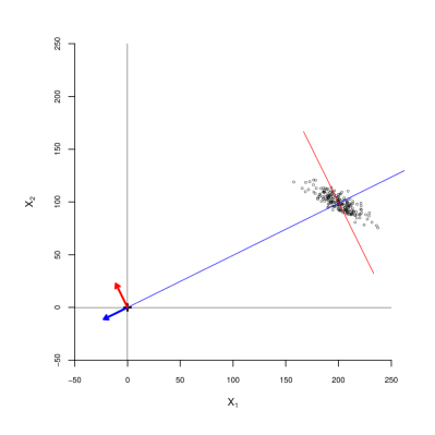
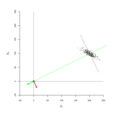
C	D

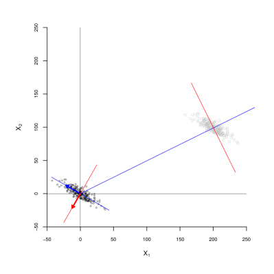
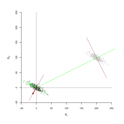
Figure 1: General Geometry of SVD and PCA. The data $\mathbf{X}$ are the cloud of points: 200 points distributed in bivariate Normal $\mathcal{N}(\mu,\Sigma),\mu=(200,100),\Sigma=$ $\left[\begin{smallmatrix}200&100\\ 100&75\end{smallmatrix}\right]$. Panel (A): New dimensions identified by SVD. Blue vector is first right singular vector $\mathbf{v}_{1}$. Red vector is second right singular vector $\mathbf{v}_{2}$. Panel (B): New dimensions identified by eigen decomposition of $\mathbf{X^{\text{T}}X}$. Green vector is first eigenvector, and brown vector is second eigenvector. Panel (C): Same as Panel (A) adding centered cloud and new dimensions identified by SVD of the centered cloud. Panel (D): Same as Panel (B) adding centered cloud and new dimensions identified by Eigen decomposition of the centered cloud. Notice (1) that the SVD of $\mathbf{X}$ and the eigen decomposition of $\mathbf{X^{\text{T}}X}$ produce exactly the same new dimensions (net of sign), (2) that the new dimensions of the ‘raw’ cloud do not line up with the primary dimensions of the raw cloud, and (3) that the new dimensions of the centered cloud do line up with the primary dimensions of the centered cloud.

3 Matrix Approximation and a useful Geometric Interpretation of the SVD

For our purposes there is another equivalent and more useful way of understanding the SVD as a sum of rank-1 matrices that can be rearranged to express each column of $\mathbf{X}$ as a weighted sum of the column vectors of $\mathbf{U}$. Below we derive this re-expression and then discuss why it is useful.

3.1 The SVD as a Sum of Rank-1 Matrices

Let the data matrix $\mathbf{X}$ be an arbitrary $K\times L$ matrix or real values with $\text{rank}(\mathbf{X})=\rho$; $\rho\leq\text{min}(K,L)$. The rank of a matrix is the number of independent rows and columns that it has; the number of columns and rows that cannot be expressed as multiplies of others. Intuitively this is the number of dimensions defined or actually occupied by the column and row vectors in the matrix. Now, let the factors of the SVD be:

• $\mathbf{U}$, a $K\times\rho$ matrix whose column vectors are the left singular vectors.

• $\mathbf{S}$, a $\rho\times\rho$ diagonal (square) matrix containing the singular values.

• $\mathbf{V}$, a $L\times\rho$ matrix whose column vectors are the right singular vectors.

Then the SVD of $\mathbf{X}$ is:

$$\mathbf{X} =\mathbf{USV}^{\text{T}}$$ (5)

$$\left[\begin{matrix}|&&|\\ \mathbf{x}_{1}&\ldots&\mathbf{x}_{L}\\ |&&|\\ \end{matrix}\right] =\left[\begin{matrix}|&&|\\ \mathbf{u}_{1}&\ldots&\mathbf{u}_{\rho}\\ |&&|\\ \end{matrix}\right]\left[\begin{matrix}s_{1}&\ldots&0\\ \vdots&\ddots&\vdots\\ 0&\ldots&s_{\rho}\\ \end{matrix}\right]\left[\begin{matrix}\text{---}&\mathbf{v}_{1}&\text{---}\\ &\vdots&\\ \text{---}&\mathbf{v}_{\rho}&\text{---}\\ \end{matrix}\right]$$

$$=\left[\begin{matrix}|&&|\\ \mathbf{u}_{1}&\ldots&\mathbf{u}_{\rho}\\ |&&|\\ \end{matrix}\right]\left[\begin{matrix}\text{---}&s_{1}\mathbf{v}_{1}&\text{---}\\ &\vdots&\\ \text{---}&s_{\rho}\mathbf{v}_{\rho}&\text{---}\\ \end{matrix}\right]$$

$$=\left[\begin{matrix}\sum_{i=1}^{\rho}u_{1i}s_{i}v_{1i}&\ldots&\sum_{i=1}^{\rho}u_{1i}s_{i}v_{Li}\\ \vdots&\ddots&\vdots\\ \sum_{i=1}^{\rho}u_{Ki}s_{i}v_{1i}&\ldots&\sum_{i=1}^{\rho}u_{Ki}s_{i}v_{Li}\\ \end{matrix}\right]$$

$$=\left[\begin{matrix}|&&|\\ \sum_{i=1}^{\rho}s_{i}v_{1i}\mathbf{u}_{i}&\ldots&\sum_{i=1}^{\rho}s_{i}v_{Li}\mathbf{u}_{i}\\ |&&|\\ \end{matrix}\right]$$ (6)

$$=\sum_{i=1}^{\rho}\left[\begin{matrix}|&&|\\ s_{i}v_{1i}\mathbf{u}_{i}&\ldots&s_{i}v_{Li}\mathbf{u}_{i}\\ |&&|\\ \end{matrix}\right]$$

$$=\sum_{i=1}^{\rho}\left[\begin{matrix}s_{i}v_{1i}u_{1i}&\ldots&s_{i}v_{Li}u_{1i}\\ \vdots&\ddots&\vdots\\ s_{i}v_{1i}u_{Ki}&\ldots&s_{i}v_{Li}u_{Ki}\\ \end{matrix}\right]$$

$$=\sum_{i=1}^{\rho}s_{i}\left[\begin{matrix}u_{1i}\\ \vdots\\ u_{Ki}\\ \end{matrix}\right]\left[\begin{matrix}v_{1i}\ldots v_{Li}\\ \end{matrix}\right]$$ (7)

$$\mathbf{X} =\sum_{i=1}^{\rho}s_{i}\mathbf{u}_{i}\mathbf{v}_{i}^{\text{T}}$$ (8)

Equation 8 expresses $\mathbf{X}$ as a sum of rank-1 matrices (each term contains a matrix constructed from a single column vector $\mathbf{u}_{i}$, hence rank-1). The Eckart-Young-Mirsky matrix approximation theorem (Golub et al., 1987) describes the fact that the matrices in this sum have the special property that they account for successively less and less of the overall variability in $\mathbf{X}$. For each $i<\rho$ in Equation 8 we can form a partial sum that is an approximation of $\mathbf{X}$, and each such sum obeys the constraint that it produces the best possible rank-$i$ approximation of $\mathbf{X}$ in a perpendicular, sum-of-squares sense, i.e. its row vectors are points that are as close as possible in a Euclidean sense to the corresponding points (row vectors) in $\mathbf{X}$ as can be achieved using $i$ dimensions. Formally, the Euclidean difference between $\mathbf{X}$ and the rank-$i$ approximation $\mathbf{X}^{[i]}$ is as small as possible. This can be expressed as (Abdi and Williams, 2010; Golub et al., 1987),

$$\Big{\lVert}\mathbf{X}-\mathbf{X}^{[i]}\Big{\rVert}^{2}=\operatorname{Tr}\left\{(\mathbf{X}-\mathbf{X}^{[i]})(\mathbf{X}-\mathbf{X}^{[i]})^{\text{T}}\right\}=\min\limits_{\mathbf{X}^{[\leq i]}}\ \Big{\lVert}\mathbf{X}-\mathbf{X}^{[\leq i]}\Big{\rVert}^{2}$$ (9)

where $\mathbf{X}^{[\leq i]}$ are matrices of rank less than or equal to $i$, and $\lVert\cdot\rVert$ is the square root of the sum of squared elements of the row vectors of matrix $\mathbf{A}$:

$$\lVert\mathbf{A}\rVert=\sqrt{\operatorname{Tr}\left(\mathbf{A}\mathbf{A}^{\text{T}}\right)}$$

Intuitively, what this means is that the first term in the sum in Equation 8 produces ‘predicted’ points that are as close as possible to the actual points (in a perpendicular sense) using just one dimension, i.e. a line. The predicted points are vectors that are multiples of the first right singular vector $\mathbf{v}_{1}$, and the extension/contraction factors that define them are $s_{1}\mathbf{u}_{1}$, easiest to see in Equation 7. The second term in the sum produces vectors that are multiples of the second right singular vector $\mathbf{v}_{2}$, similarly with weights equal to $s_{2}\mathbf{u}_{2}$, that when added to the vectors defined by the first term produce predicted points that are a little closer to the actual points. This pattern continues through the sum until the last term adds multiples of the last right singular vector and finally completes a vector sum that reproduces the actual points exactly.

Because each successive approximation gets as close as possible to the actual points using the orthonormal basis $\mathbf{V}$, the first few terms cover most of the distance from the origin to the actual points, and the remaining terms make comparatively small and often negligible contributions. It is this property of the sum that makes it useful – the original data matrix $\mathbf{X}$ can be closely approximated by a sum with (possibly many) fewer terms than the rank of $\mathbf{X}$. Figure 2 is a convincing visual display of this property of Equation 8.

There are two final points to note. The approximation condition defined in Equation 9 implies that each term in Equation 8 is associated with a fraction of the overall ‘perpendicular’ squared (Euclidean) distance from the origin to the points. The first term minimizes the difference between the points and their best approximation along a single line, or conversely, maximizes the share of the overall perpendicular squared distance from the origin to the points accounted for by the one-term approximation. The remaining terms account for smaller and smaller fractions of this overall perpendicular squared distance. The perpendicular squared distance accounted for by each term is equal to the square of the singular value corresponding to that term. This fact ensures that the singular values are always arranged in a monotonically decreasing list: $s_{1}\geq s_{2}\ldots\geq s_{\rho}$, and unless the cloud of data points is centered, $s_{1}$ is much larger than the rest, and the first few are much larger than the others. The singular values are the fraction of the total squared distance from the origin to all of the points that is ‘accounted for’ by each new dimension $\mathbf{v}_{i}$. This contribution can be quantified by calculating the square of each singular value and dividing that by the sum of the squares of the singular values.

Finally, it is worth reiterating and stating explicitly that Equation 9 ensures that the right singular vectors $\mathbf{V}$ point in the directions of maximum variation in the original cloud of points defined by $\mathbf{X}$, subject to the constraint that they remain perpendicular, and that the overall perpendicular distance starts from the origin. The last condition is why data clouds must be centered in order for the right singular vectors to point in directions that correspond to the dominant orthogonal dimensions of the cloud and why PCA is conducted on centered data.

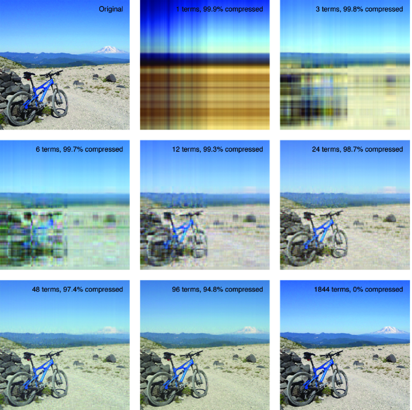
Figure 2: Illustration of the Reduced-rank Approximation using an Image. The top left panel contains the original $1,844\times 1,852$ color image of Mt. Adams from the east flank of Mt. St. Helens. The image is a three-dimension array containing one $1,844\times 1,852$ matrix of $\left[0,1\right]$ values (one value for each pixel) for each primary color red, blue and green. The SVD was used to decompose each of the three matrices, and then they are reconstructed using the number of terms in Equation 8 indicated in their label. The image in the lower right panel uses the maximum number of components (1,844) and reproduces the original exactly. With just 6 components (0.3% of the information in the original, or 99.7% compressed) all fundamental aspects of the image are in place, the colors are close to their correct values, and it is possible to detect that there is a bicycle in the photo; with just 24 components (98.7% compressed) the entire scene is interpretable with high confidence, and with 96 components (94.8% compressed) you would not know you are missing most of the original.

3.2 Each Column of the Data Matrix as a Sum of Left Singular Vectors

Interpreting the SVD as a sum of rank-1 matrices leads directly to a similar and very useful expression for each of its column vectors. In the derivation above, just before converting to a sum of matrices, we express the SVD as a matrix of sums, one for each column. Equation 6 says that each column vector $\mathbf{x}_{\ell}$ in $\mathbf{X}$ can be written

$$\mathbf{x}_{\ell}=\sum_{i=1}^{\rho}s_{i}v_{\ell,i}\mathbf{u}_{i}\ .$$ (10)

This is the key equation that we have been building up to. Equation 10 says that we can write all the columns in $\mathbf{X}$ as weighted sums of the left singular vectors scaled by their corresponding singular values, and it tells us what the weights are, namely the $\ell^{\text{th}}$ elements of each corresponding right singular vector. Moreover, because of the nature of the reduced-rank approximations described above, we know that these sums have the property of concentrating most of the variation in the first few terms, and consequently we only need the first few terms to produce predicted values that are very close to the actual values. This allows us to closely approximate the columns of $\mathbf{X}$ with (potentially very) few effective parameters – just the first few weights.

3.3 A Parsimonious Model and Smoother for Vectors Similar to the Columns of the Data Matrix

Equation 10 suggests the form of a parsimonious model for an arbitrary column vector of the same length and similar to the columns of $\mathbf{X}$, namely

$$\widehat{\mathbf{x}} =\sum_{i=1}^{c}\beta_{i}\cdot s_{i}\mathbf{u}_{i}\ ,$$ (11)

$$\mathbf{x} =\widehat{\mathbf{x}}+\mathbf{r}\ .$$

where the $\beta_{i}$ are chosen to minimize the magnitude of the residual $\lVert\mathbf{r}\rVert$; $\mathbf{r}$ is the difference between $\mathbf{x}$ and its predicted value $\widehat{\mathbf{x}}$ using $c\leq\rho$ components.

In addition to serving as a reduced-dimension, compact model for $\mathbf{x}$, Equation 11 can also be thought of as a smoother. By not including the higher-order, small magnitude terms in the sum, it is possible to eliminate the small, less systematic, mostly stochastic differences between the elements in $\mathbf{x}$. What is left when only the first few terms are included are the systematic differences between the elements of $\mathbf{x}$ that are shared by all or the majority of the column vectors in the data matrix whose SVD produced the singular values and left singular vectors used in Equation 11 to produce the approximation of $\mathbf{x}$. This is a common use of SVD that has been applied in many fields for many purposes, e.g. signal processing, image compression and clustering.

3.4 A Simple $3\times 2$ Example SVD with Geometric Interpretation

Equation 12 defines the general SVD of a simple $3\times 2$ matrix $\mathbf{X}$ in detail, and Equations 13 (detailed) and 15 (compact) describe the component form of the SVD for this particular case. Let:

$$\mathbf{X} =\left[\begin{matrix}x_{11}&x_{12}\\ x_{21}&x_{22}\\ x_{31}&x_{32}\\ \end{matrix}\right], \mathbf{x}_{i} =\left[\begin{matrix}x_{1i}\\ x_{2i}\\ x_{3i}\\ \end{matrix}\right]$$

$$\mathbf{U} =\left[\begin{matrix}u_{11}&u_{12}\\ u_{21}&u_{22}\\ u_{31}&u_{32}\\ \end{matrix}\right], \mathbf{u}_{i} =\left[\begin{matrix}u_{1i}\\ u_{2i}\\ u_{3i}\\ \end{matrix}\right]$$

$$\mathbf{S} =\left[\begin{matrix}s_{1}&0\\ 0&s_{2}\\ \end{matrix}\right]$$

$$\mathbf{V} =\left[\begin{matrix}v_{11}&v_{12}\\ v_{21}&v_{22}\\ \end{matrix}\right], \mathbf{v}_{i} =\left[\begin{matrix}v_{1i}\\ v_{2i}\\ \end{matrix}\right]$$

Then the SVD of $\mathbf{X}$ is

$$\mathbf{X} =\mathbf{USV}^{\text{T}}$$

$$\left[\begin{matrix}x_{11}&x_{12}\\ x_{21}&x_{22}\\ x_{31}&x_{32}\\ \end{matrix}\right] =\left[\begin{matrix}u_{11}&u_{12}\\ u_{21}&u_{22}\\ u_{31}&u_{32}\\ \end{matrix}\right]\left[\begin{matrix}s_{1}&0\\ 0&s_{2}\\ \end{matrix}\right]\left[\begin{matrix}v_{11}&v_{21}\\ v_{12}&v_{22}\\ \end{matrix}\right]$$ (12)

$$=\left[\begin{matrix}u_{11}&u_{12}\\ u_{21}&u_{22}\\ u_{31}&u_{32}\\ \end{matrix}\right]\left[\begin{matrix}s_{1}v_{11}&s_{1}v_{21}\\ s_{2}v_{12}&s_{2}v_{22}\\ \end{matrix}\right]$$

$$=\left[\begin{matrix}u_{11}s_{1}v_{11}+u_{12}s_{2}v_{12}&u_{11}s_{1}v_{21}+u_{12}s_{2}v_{22}\\ u_{21}s_{1}v_{11}+u_{22}s_{2}v_{12}&u_{21}s_{1}v_{21}+u_{22}s_{2}v_{22}\\ u_{31}s_{1}v_{11}+u_{32}s_{2}v_{12}&u_{31}s_{1}v_{21}+u_{32}s_{2}v_{22}\\ \end{matrix}\right]$$

$$=\left[\begin{matrix}s_{1}v_{11}\left[\begin{matrix}u_{11}\\ u_{21}\\ u_{31}\\ \end{matrix}\right]+s_{2}v_{12}\left[\begin{matrix}u_{12}\\ u_{22}\\ u_{32}\\ \end{matrix}\right]&s_{1}v_{21}\left[\begin{matrix}u_{11}\\ u_{21}\\ u_{31}\\ \end{matrix}\right]+s_{2}v_{22}\left[\begin{matrix}u_{12}\\ u_{22}\\ u_{32}\\ \end{matrix}\right]\\ \end{matrix}\right]$$ (13)

$$=\left[\begin{matrix}s_{1}v_{11}\left[\begin{matrix}u_{11}\\ u_{21}\\ u_{31}\\ \end{matrix}\right]&s_{1}v_{21}\left[\begin{matrix}u_{11}\\ u_{21}\\ u_{31}\\ \end{matrix}\right]\\ \end{matrix}\right]+\left[\begin{matrix}s_{2}v_{12}\left[\begin{matrix}u_{12}\\ u_{22}\\ u_{32}\\ \end{matrix}\right]&s_{2}v_{22}\left[\begin{matrix}u_{12}\\ u_{22}\\ u_{32}\\ \end{matrix}\right]\\ \end{matrix}\right]$$ (14)

$$=\left[\begin{matrix}s_{1}v_{11}u_{11}&s_{1}v_{21}u_{11}\\ s_{1}v_{11}u_{21}&s_{1}v_{21}u_{21}\\ s_{1}v_{11}u_{31}&s_{1}v_{21}u_{31}\end{matrix}\right]+\left[\begin{matrix}s_{2}v_{12}u_{12}&s_{2}v_{22}u_{12}\\ s_{2}v_{12}u_{22}&s_{2}v_{22}u_{22}\\ s_{2}v_{12}u_{32}&s_{2}v_{22}u_{32}\end{matrix}\right]$$

$$=s_{1}\left[\begin{matrix}u_{11}\\ u_{21}\\ u_{31}\\ \end{matrix}\right]\left[\begin{matrix}v_{11}&v_{21}\\ \end{matrix}\right]+s_{2}\left[\begin{matrix}u_{12}\\ u_{22}\\ u_{32}\\ \end{matrix}\right]\left[\begin{matrix}v_{12}&v_{22}\\ \end{matrix}\right]$$

$$\mathbf{X} =\sum_{i=1}^{2}s_{i}\mathbf{u}_{i}\mathbf{v}_{i}^{\text{T}}$$ (15)

From (13)

$$\mathbf{x}_{1} =s_{1}v_{11}\left[\begin{matrix}u_{11}\\ u_{21}\\ u_{31}\\ \end{matrix}\right]+s_{2}v_{12}\left[\begin{matrix}u_{12}\\ u_{22}\\ u_{32}\\ \end{matrix}\right]$$

$$\mathbf{x}_{1} =s_{1}v_{11}\mathbf{u}_{1}+s_{2}v_{12}\mathbf{u}_{2}$$ (16)

and

$$\mathbf{x}_{2} =s_{1}v_{21}\left[\begin{matrix}u_{11}\\ u_{21}\\ u_{31}\\ \end{matrix}\right]+s_{2}v_{22}\left[\begin{matrix}u_{12}\\ u_{22}\\ u_{32}\\ \end{matrix}\right]$$

$$\mathbf{x}_{2} =s_{1}v_{21}\mathbf{u}_{1}+s_{2}v_{22}\mathbf{u}_{2}$$ (17)

Following this general form, below we work an example with three specific points in two dimensions. Figure 3 displays the three example points: (2,1) labeled ‘1’, (1,1) labeled ‘2’ and (1,2) labeled ‘3’.

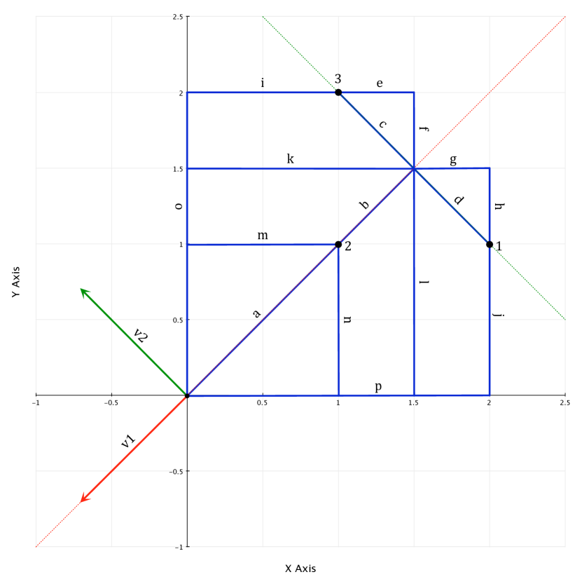
Figure 3: $3\times 2$ Example. The ‘data matrix’ consists of the three points labeled ‘1’, ‘2’ and ‘3’. The right singular vectors $\mathbf{V}$ are red and green and labeled ‘v1’ and ‘v2’; they define the new orthogonal basis associated with the SVD of the three points. The blue line segments mark distances that are used in the calculation of the SVD and are labeled with letters from the alphabet. Segments ‘a’, ‘a+b’, ‘c’ and ‘d’ are proportional to the left singular vectors of the SVD (scaled by the singular values).

The line segments necessary to demonstrate the SVD are labeled $a$ – $p$, and the lengths of each are:

$$a =\sqrt{2}\ , c =\tfrac{\sqrt{2}}{2}\ , e =-0.5\ , g =\phantom{-}0.5\ , i =1\ , k =1.5\ , m =1\ , o =2$$

$$b =\tfrac{\sqrt{2}}{2}\ , d =\tfrac{\sqrt{2}}{2}\ , f =\phantom{-}0.5\ , h =-0.5\ , j =1\ , l =1.5\ , n =1\ , p =2$$

First, we identify the singular vectors $\mathbf{v}_{1}$ and $\mathbf{v}_{2}$. The requirement is that the first singular vector point in a direction that maximizes the sum of squared distances along this dimension to all of the points, or conversely, minimizes the sum of squared differences between the points and their predicted values, i.e. their projections onto this new dimension. Given the simplicity and symmetry of this example, we can readily see that $\mathbf{v}_{1}$ must be in the direction of the red vector labeled ‘v1’ in Figure 3. The projections of point 1 (2,1) and 3 (1,2) onto this new dimension are both the point where line segments b, c, d, f, g, k & l meet, and point 2 (1,1) actually lies on this dimension already. A final requirement is that the length of the singular vectors be 1, so we choose the point $\big{(}-\sqrt{0.5},-\sqrt{0.5}\big{)}$ to define $\mathbf{v}_{1}$, whether it points down and the left or up and to the right does not matter, and it is easier to see in the figure if we define it like this.

$\mathbf{v}_{2}$ must be perpendicular to $\mathbf{v}_{1}$, and the only option in this two-dimension example is along the direction of the green vector labeled ‘v2’ in Figure 3. We choose $\mathbf{v}_{2}$ defined by $\big{(}-\sqrt{0.5},\sqrt{0.5}\big{)}$, again to ensure its magnitude is 1.

Second, we calculate the singular values $s_{1}$ and $s_{2}$ and demonstrate how these are related to the total sum of squares. The total sum of squares is the sum of squared perpendicular distances from the origin along each original dimension $X,Y$ to the three points, in order 1–3:

$$SS_{tot} =\bigl{(}p^{2}+j^{2}\bigr{)}+\bigl{(}m^{2}+n^{2}\bigr{)}+\bigl{(}i^{2}+o^{2}\bigr{)}$$ (18)

$$=4+1+1+1+1+4=12$$

The first singular value $s_{1}$ is the square root of the sum of squared distances from the origin to each point on the dimension defined by the first singular vector $\mathbf{v}_{1}$, again in order 1–3:

$$s_{1}^{2}=SS_{1} =\bigl{(}a+b\bigr{)}^{2}+a^{2}+\bigl{(}a+b\bigr{)}^{2}$$ (19)

$$=\big{(}\tfrac{3}{2}\sqrt{2}\big{)}^{2}+\bigl{(}\sqrt{2}\bigr{)}^{2}+\big{(}\tfrac{3}{2}\sqrt{2}\big{)}^{2}$$

$$=\tfrac{9}{2}+\tfrac{4}{2}+\tfrac{9}{2}$$

$$=\tfrac{22}{2}=11$$

$$\rightarrow s_{1} =\sqrt{11}=3.3166$$

The second singular value $s_{2}$ is the square root of the sum of squared distances from the projection of the points onto the first new dimension ($\mathbf{v}_{1}$) to each point along the dimension defined by the second singular vector $\mathbf{v}_{2}$ (i.e. segment $d$ for point 1, 0 for point 2 and segment $c$ for point 3), in order 1–3:

$$s_{2}^{2}=SS_{2} =d^{2}+0^{2}+c^{2}$$ (20)

$$=\Big{(}\tfrac{\sqrt{2}}{2}\Big{)}^{2}+0+\Big{(}\tfrac{\sqrt{2}}{2}\Big{)}^{2}$$

$$=\tfrac{1}{2}+\tfrac{1}{2}=1$$

$$\rightarrow s_{2} =\sqrt{1}=1$$

We can verify that the sum of the squares of the singular values is equal to the total sum of squares.

$$SS_{1}+SS_{2} =s_{1}^{2}+s_{2}^{2}$$ (21)

$$=11+1=12\ \checkmark$$

$$=SS_{tot}$$ (22)

Using the original $X,Y$ dimensions, the sum of squared perpendicular distances associated with either the $X$ or $Y$ dimension is $\left(p^{2}+m^{2}+i^{2}\right)$ or $\left(j^{2}+n^{2}+o^{2}\right)=\left(1^{2}+1^{2}+2^{2}\right)=6$, or 12 for both dimensions combined. The SVD identifies a new set of dimensions such that a majority of the squared distance to the points is along the ‘primary’ new dimension and the remainder along the secondary new dimension(s), in this case 11 along the first and 1 along the second.

Finally, we identify the left singular vectors $\mathbf{u}_{1}$ and $\mathbf{u}_{2}$. From the first term in Equation 14 we see that the product of $\mathbf{u}_{1}$ and the first singular value $s_{1}$ multiplies (extends or contracts) the $X$ and $Y$ elements of $\mathbf{v}_{1}$, and similarly, the product of $\mathbf{u}_{2}$ and the second singular value $s_{2}$ multiplies the $X$ and $Y$ elements of $\mathbf{v}_{2}$. To calculate the values of the elements of $\mathbf{u}_{1}$ we take the $X$ and $Y$ distances to the projections of the points along the the first right singular vector $\mathbf{v}_{1}$ and divide them by $s_{1}v_{11}$ in the case of the $X$ dimension or $s_{1}v_{21}$ for the $Y$ dimension. Using values from the example along the $X$ dimension:

$$u_{11} =\frac{k}{s_{1}v_{11}}=\frac{1.5}{\sqrt{11}\times-\sqrt{0.5}}=-0.6396$$

$$u_{21} =\frac{m}{s_{1}v_{11}}=\frac{1}{\sqrt{11}\times-\sqrt{0.5}}=-0.4264$$

$$u_{31} =\frac{k}{s_{1}v_{11}}=\frac{1.5}{\sqrt{11}\times-\sqrt{0.5}}=-0.6396$$

or, using the $Y$ dimension:

$$u_{11} =\frac{\ell}{s_{1}v_{21}}=\frac{1.5}{\sqrt{11}\times-\sqrt{0.5}}=-0.6396$$

$$u_{21} =\frac{n}{s_{1}v_{21}}=\frac{1}{\sqrt{11}\times-\sqrt{0.5}}=-0.4264$$

$$u_{31} =\frac{\ell}{s_{1}v_{21}}=\frac{1.5}{\sqrt{11}\times-\sqrt{0.5}}=-0.6396$$

The result is the same in both cases, as it must be.

Similarly from Equation 14 we see that $\mathbf{u}_{2}$ multiplies the $X$ and $Y$ elements of $\mathbf{v}_{2}$ to create vectors in the $\mathbf{v}_{2}$ direction that when added to the vectors produced by extending $\mathbf{v}_{1}$ by $\mathbf{u}_{1}$ yield the original points. This time the numerators may have a negative sign because we are projecting the vectors obtained by subtracting the extended versions of $\mathbf{v}_{1}$ described just above from the original points, and the resulting vectors are not all in the 1${}^{\text{st}}$ quadrant. Again using values from the example in the $X$ dimension:

$$u_{12} =\frac{g}{s_{2}v_{12}}=\frac{0.5}{1\times-\sqrt{0.5}}=-0.7071$$

$$u_{22} =\frac{0}{s_{2}v_{12}}=\frac{0}{1\times-\sqrt{0.5}}=\phantom{-}0$$

$$u_{32} =\frac{e}{s_{2}v_{12}}=\frac{-0.5}{1\times-\sqrt{0.5}}=\phantom{-}0.7071$$

or, using the $Y$ dimension:

$$u_{12} =\frac{h}{s_{2}v_{22}}=\frac{-0.5}{1\times\sqrt{0.5}}=-0.7071$$

$$u_{22} =\frac{0}{s_{2}v_{22}}=\frac{0}{1\times\sqrt{0.5}}=\phantom{-}0$$

$$u_{32} =\frac{f}{s_{2}v_{22}}=\frac{0.5}{1\times\sqrt{0.5}}=\phantom{-}0.7071$$

Again, the result is the same either way.

Summarizing our intuitive, geometric calculation of the SVD of $\mathbf{X}$:

$$\mathbf{X} =\left[\begin{matrix}2&1\\ 1&1\\ 1&2\\ \end{matrix}\right] \mathbf{U} =\left[\begin{matrix}-0.6396&-0.7071\\ -0.4264&0\\ -0.6396&\phantom{-}0.7071\\ \end{matrix}\right]$$

$$\mathbf{S} =\left[\begin{matrix}3.3166&0\\ 0&1\\ \end{matrix}\right] \mathbf{V} =\left[\begin{matrix}-0.7071&-0.7071\\ -0.7071&\phantom{-}0.7071\\ \end{matrix}\right]$$

Using the statistical package R to calculate the SVD of $\mathbf{X}$ yields:

$$\mathbf{X} =\left[\begin{matrix}2&1\\ 1&1\\ 1&2\\ \end{matrix}\right] \mathbf{U} =\left[\begin{matrix}-0.6396021&\phantom{1}7.071068\text{e-01}\\ -0.4264014&\phantom{1}2.775558\text{e-17}\\ -0.6396021&-7.071068\text{e-01}\\ \end{matrix}\right]$$

$$\mathbf{S} =\left[\begin{matrix}3.316625&0\\ 0&1.000000\\ \end{matrix}\right] \mathbf{V} =\left[\begin{matrix}-0.7071068&\phantom{-}0.7071068\\ -0.7071068&-0.7071068\\ \end{matrix}\right]$$

The results are effectively identical; the SVD algorithm in R chose to point $\mathbf{v}_{2}$ in the opposite direction which caused the signs on the members of $\mathbf{u}_{2}$ to flip; equivalent to our result.

Looking more closely at $\mathbf{U}$, we can begin to see how the SVD can be useful in demography. $\mathbf{u}_{1}$ in the direction of the points, i.e. $-1\times\mathbf{u}_{1}=\left[\begin{smallmatrix}0.64\\ 0.43\\ 0.64\end{smallmatrix}\right]$, encodes the ‘shape’ of the points along $\mathbf{v}_{1}$. Starting with point 1, we go out, then come back in for point 2, and finally back out again for point 3. If the dimension defined by $\mathbf{v}_{1}$ is age-specific, then $\mathbf{u}_{1}$ is a scaled age pattern.

Finally, turning our attention back to Equations 16 and 17, we see that the column vectors of $\mathbf{X}$ are expressed as weighted sums of the $\mathbf{u}$’s scaled by their corresponding singular values, and the weights are the elements of the row vectors of $\mathbf{V}$. Each term in these sums is a fraction of the distance along the original $X$ and $Y$ axes from the origin to our three points. Because the first left singular vector is associated with the new basis direction along which there is most ‘squared distance’ from the origin, the first term in these weighted sums represents the largest fraction, with subsequent terms accounting for smaller and smaller fractions. This allows us to approximate the column vectors in $\mathbf{X}$ with a subset of the terms in these weighted sums. In our two-dimension example, we have just two terms; with the first we have a reasonable approximation of the column vectors of $\mathbf{X}$, and with both we reproduce them exactly. In this re-expression, the first column vector $\mathbf{x}_{1}$ is

$${\mathbf{x}_{1}} =\left[\begin{matrix}2\\ 1\\ 1\\ \end{matrix}\right]=s_{1}v_{11}\left[\begin{matrix}u_{11}\\ u_{21}\\ u_{31}\\ \end{matrix}\right]+s_{2}v_{12}\left[\begin{matrix}u_{12}\\ u_{22}\\ u_{32}\\ \end{matrix}\right]$$

$$=3.3166\times-0.7071\left[\begin{matrix}-0.6396\\ -0.4264\\ -0.6396\\ \end{matrix}\right]+1\times-0.7071\left[\begin{matrix}-0.7071\\ \phantom{-0.707}0\\ \phantom{-}0.7071\\ \end{matrix}\right]$$

$$=\left[\begin{matrix}1.5\\ \phantom{1.}1\\ 1.5\\ \end{matrix}\right]+\left[\begin{matrix}\phantom{-}0.5\\ \phantom{-0.}0\\ -0.5\\ \end{matrix}\right]=\left[\begin{matrix}2\\ 1\\ 1\\ \end{matrix}\right]\ \checkmark$$

The first term in this sum $\left[\begin{smallmatrix}1.5\\ \phantom{1.}1\\ 1.5\\ \end{smallmatrix}\right]$ approximates $\mathbf{x}_{1}$ quite well, and the second $\left[\begin{smallmatrix}\phantom{-}0.5\\ \phantom{-0.}0\\ -0.5\\ \end{smallmatrix}\right]$ makes the small refinement necessary to reproduce $\mathbf{x}_{1}$ exactly. In this example the situation is very similar for the second column vector $\mathbf{x}_{2}$, the only difference being in the second term.

$${\mathbf{x}_{2}} =\left[\begin{matrix}1\\ 1\\ 2\\ \end{matrix}\right]=s_{1}v_{21}\left[\begin{matrix}u_{11}\\ u_{21}\\ u_{31}\\ \end{matrix}\right]+s_{2}v_{22}\left[\begin{matrix}u_{12}\\ u_{22}\\ u_{32}\\ \end{matrix}\right]$$

$$=3.3166\times-0.7071\left[\begin{matrix}-0.6396\\ -0.4264\\ -0.6396\\ \end{matrix}\right]+1\times 0.7071\left[\begin{matrix}-0.7071\\ \phantom{-0.707}0\\ \phantom{-}0.7071\\ \end{matrix}\right]$$

$$=\left[\begin{matrix}1.5\\ \phantom{1.}1\\ 1.5\\ \end{matrix}\right]+\left[\begin{matrix}-0.5\\ \phantom{-0.}0\\ \phantom{-}0.5\\ \end{matrix}\right]=\left[\begin{matrix}1\\ 1\\ 2\\ \end{matrix}\right]\ \checkmark$$

In both cases we are almost all the way there with just the first term.

4 The SVD and Demographic Quantities Correlated by Age

In this section we turn to a practical application of the SVD in demography.

4.1 Demographic Quantities Correlated by Age – Age Schedules

Various demographic quantities including age-specific mortality and fertility are correlated by age. The data used in the examples in the Section 5 is displayed in Figure 8 and reveal the very strong age-dependance that is typical for both mortality and fertility. The pair-wise correlation coefficients for the two-sex (female joined to male in one 38-element vector) age-specific log mortality schedules plotted in Figure 8 are $\geq 0.90$ in all cases. Likewise the log age-specific fertility schedules have pair-wise correlation coefficients that are no less than 0.99.

This feature of many age-specific demographic quantities makes them amenable to direct decomposition using the SVD. Imagine organizing the age schedules into a matrix $\mathbf{A}$ so that each age schedule is a column and each age (group) is a row; a $G\times H$ matrix of age-specific quantities. Geometrically, each of the $G$ rows in this matrix corresponds to a point in $H$-dimension space, and together the points defined by the rows make up the cloud of data points that we want to characterize using the SVD. In order to make the SVD interpretable and to retain the original scale of our data so that we can model them without translation (e.g. centering) or rescaling (e.g. normalizing), we need to be sure that the primary dimension identified by the SVD – the first right singular vector $\mathbf{v}_{1}$ – is lined up with the dimension of maximum variability in the cloud of points representing our age schedules. Remember that the first right singular vector points from the origin to the center of the cloud, which means that the primary dimension of the cloud must be or be very similar to the first right singular vector in order to make the SVD of the uncentered cloud useful.

The fact that demographic age schedules are correlated by age and none are offset, or moved, along the age axis means that the distance from the origin to each point along each of the $H$ axes is similar, that is, the points in $\mathbf{A}$ all lie roughly on a line that intersects the origin and has ‘slope’ $\approx$ 1. Of course when the number of columns exceeds three, one cannot visualize this line, but the fact still holds for an arbitrary number of dimensions (columns).

This can be seen easily by imagining just two age schedules. In that case we have a simple two-column, two-dimension data set that corresponds to a cloud of $G$ points on a familiar two-dimension $X$, $Y$ plot. Now imagine plotting the points that correspond to the age schedules. Because the values are similar for each age group, the distance along both axes is similar for every point, and all the points cluster around a line with slope $\approx$ 1, see Panel (A) in Figure 4.

It is also generally true that the primary dimension identified by the first right singular vector also captures the vast majority of the variation in the cloud of points. This is obvious when one notes that this dimension effectively captures the level or magnitude of the indicator by age, the differences that are on the vertical axis if each age schedule were plotted by age. The remaining orthogonal axes identified by the remaining right singular vectors capture the remaining variability in the cloud; variability that is age-specific but largely unrelated to the overall level or magnitude of the age schedule.

Figures 4 and 5 display an example of the geometry of the SVD using two mortality age schedules from the example data listed in Appendix A Table A.6.

A: Log Mortality Rate Cloud	B: Geometry of Female Point 7

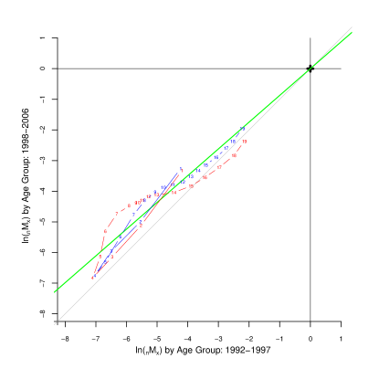
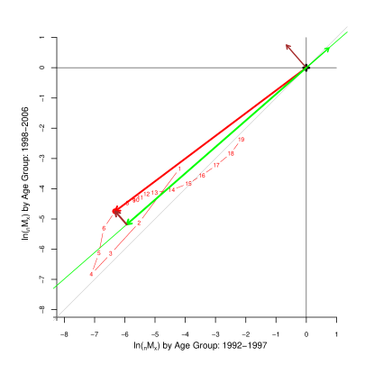
Figure 4: Two-dimension Example – Geometry of SVD. Panel (A): Scatterplot of 1998–2006 life table by 1992–1997 life table. Red = female, Blue = male. Points numbered from youngest to oldest age group. Grey line is $y=x$. Green line is direction along which there is most variation in the cloud of points. Panel (B): SVD-defined vectors that reconstruct female point number 7. Small green vector pointing up and to right from origin is first right singular vector $\mathbf{v}_{1}$; small brown vector pointing up and to left from origin is second right singular vector $\mathbf{v}_{2}$. Long green vector pointing down and to left is projection along $\mathbf{v}_{1}$ corresponding to female point 7, and short brown vector from the tip of the long green vector to female point 7 is the projection along $\mathbf{v}_{2}$ corresponding to female point 7. Adding the two projections of the right singular vectors produces the long red vector from the origin down and to the left that defines female point 7.

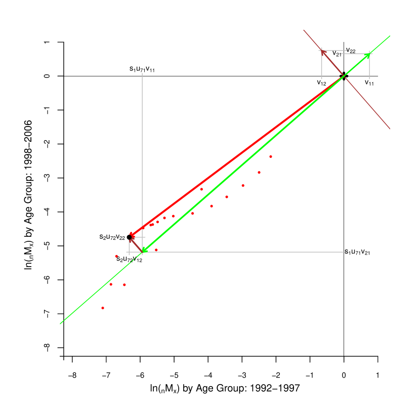
Figure 5: Two-dimension Example – Geometry of SVD, continued. Scatterplot of 1998–2006 life table by 1992–1997 life table. Red = female, Blue = male. Green line is direction along which there is most variation in the cloud of points. SVD-defined vectors that reconstruct female point number 7: small green vector pointing up and to right from origin is first right singular vector $\mathbf{v}_{1}$; small brown vector pointing up and to left from origin is second right singular vector $\mathbf{v}_{2}$. Long green vector pointing down and to left is projection along $\mathbf{v}_{1}$ corresponding to female point 7, and short brown vector from the tip of the long green vector to female point 7 is the projection along $\mathbf{v}_{2}$ corresponding to female point 7. Adding the two projections of the right singular vectors produces the long red vector from the origin down and to the left that defines female point 7. Each vector defined in terms of the original $X$, $Y$ coordinate system. This makes clear that the projections ‘stretch’ the right singular vectors by mulitplicative factors specified in the left singular vectors $\mathbf{u}$.

In summary, the first right singular vector $\mathbf{v}_{1}$ will always identify a dimension that is close to the primary dimension of the cloud of points defined by the age schedules, and this dimension will be associated with the overall level of the indicator by age. Additional orthogonal dimensions identified by the remaining right singular vectors will capture the remaining variability, most of which will be age-specific but not closely related to the overall level of the age schedules.

4.2 A General, Parsimonious, SVD-derived Model for Demographic Quantities Correlated by Age

Demography is largely about understanding the structure and dynamics of populations, and a key underlying dimension of ‘structure’ is age. Consequently demographers measure and manipulate age schedules of various quantitates – e.g. mortality, fertility, nuptially, migration, etc. – in many ways. To make these tasks easier, and to make it possible to relate age schedules as a whole (i.e. an indicator across all ages) to various covariates or predictors, it is desirable to have parsimonious models of complete age structures that can incorporate covariates. These can then be used to:

• smooth noisy age schedules,

• fill-in or extend incompletely measured age schedules, and/or

• produce full age schedules using one or a small number of parameters and/or predictors of those parameters.

The objective of the model we develop below is to provide a general modeling framework for whole age structures that requires very few (usually just two or three) parameters. A framework of this type can then be used to summarize the empirical regularities in any collection of age schedules correlated by age, and further the parameter values that replicate the observed age schedules can be themselves modeled as functions of covariates. Those models can then be used to generate parameter values from the covariates, which can in turn can be turned into full age schedules by the model. The final result is an empirical model that can be driven either directly by the parameters themselves or by the covariates used to generate parameter values. This provides a mechanism by which to predict full age schedules from the covariates.

4.2.1 Data and Model Objectives

As above, the data consist of a $G\times H$ matrix $\mathbf{A}$ of age-specific quantities. The columns of $\mathbf{A}$ correspond to the age schedules, and the rows contain the values of the indicator for each age or age group. Each row is a point in $\text{R}^{H}$ corresponding to an age group; the number of points equals to the number of ages or age groups. The objective of our model is to summarize the shape of the cloud of points as parsimoniously as possible using well-behaved and interpretable parameters. A secondary objective is to be able to remove random ‘noise,’ i.e. stochastic variation, that is not systematically related to either age or anything else. Finally, we would like to be able to identify natural groups or clusters of these points, if they exist. Cleanly separated clusters would indicate that there are groups of age schedules that are similar to one another but systematically different from all the others. If true, this is an important feature of the empirical data that likely results from some underlying mechanism (that could be explained) and can be exploited to improve our ability to both fit and predict age schedules using the model.

4.2.2 The Model – Summarizing Empirical Regularities

Given a $G\times H$ matrix $\mathbf{A}$ of age schedules, the SVD of $\mathbf{A}$ yields a set of age-varying components and corresponding weights that can be used to reconstruct the $h\in\{1\ldots H\}$ individual age schedules in $\mathbf{A}$ to within arbitrary precision using a weighted sum based on the Eckart-Young-Mirsky formula,

$$\widehat{\mathbf{a}}_{h} =\sum_{i=1}^{c}{v}{{}_{hi}}\cdot{s}{{}_{i}}{\mathbf{u}}{{}_{i}}\ ,$$ (23)

$$\mathbf{a}_{h} =\widehat{\mathbf{a}}_{h}+\mathbf{r}_{h}\ .$$

where $\mathbf{r}_{h}$ is a residual; ${v}{{}_{hi}}$, ${s}{{}_{i}}$ and ${\mathbf{u}}{{}_{i}}$ come from the SVD of $\mathbf{A}$; and $c$ is chosen so that $\lVert\mathbf{r}_{h}\rVert$ is small enough to satisfy the desired level of precision. Taking the age-varying components $\left({s}{{}_{i}}{\mathbf{u}}{{}_{i}}\right)$ as fixed, Equation 23 is a $c$-parameter model for the age schedules in $\mathbf{A}$. Because of the concentration of variation in the first few new dimensions $\left(\mathbf{V}\right)$ of the SVD, $\widehat{\mathbf{a}}_{h}$ is a smoothed or de-noised version of $\mathbf{a}_{h}$, and experience indicates that in most cases $c\leq 3$ is sufficient to adequately reproduce all of the $\mathbf{a}_{h}$. For a given matrix of age schedules $\mathbf{A}$ Equation 23 will have very high ‘within sample’ validity, i.e. it will be able to reproduce all of the $\mathbf{a}_{h}$ in $\mathbf{A}$ to within arbitrary precision (by adjusting $c$).

Equation 23 is also useful in an ‘out of sample’ sense to represent age schedules that are not included in $\mathbf{A}$, as long as they are similar to those in $\mathbf{A}$. Geometrically a new age schedule adds a new dimension to our cloud of $H$ points, and to be similar to the age schedules in $\mathbf{A}$, this new dimension has to preserve the overall shape of the cloud rather than pulling or pushing it in a new way, i.e. having lower or higher indicator values at a given age compared to the schedules in $\mathbf{A}$. This is unlikely to be a problem if $\mathbf{A}$ is large and diverse with respect to age schedules.

When used in this out-of-sample way, Equation 23 needs to be modified to specify that the age-varying components come from the SVD of a particular matrix of age schedules $\mathbf{A}$, and further that although the weights do not come from the SVD of $\mathbf{A}$ they are defined with respect to the age-varying components from $\mathbf{A}$,

$$\tensor[_{A}]{\widehat{\mathbf{a}}}{} =\sum_{i=1}^{c}\tensor[_{A}]{\beta}{{}_{i}}\cdot\tensor[_{A}]{\mathbf{\Lambda}}{{}_{i}}\ ,$$ (24)

$$\mathbf{a} =\tensor[_{A}]{\widehat{\mathbf{a}}}{}+\tensor[_{A}]{\mathbf{r}}{}\ .$$

where $\tensor[_{A}]{\mathbf{r}}{}$ is a residual; the $\tensor[_{A}]{\mathbf{\Lambda}}{{}_{i}}=\tensor[_{A}]{s}{{}_{i}}\tensor[_{A}]{\mathbf{u}}{{}_{i}}$ and come from the SVD of $\mathbf{A}$; and the $\tensor[_{A}]{\beta}{{}_{i}}$ are chosen to minimize $\lVert\tensor[_{A}]{\mathbf{r}}{}\rVert$ for a given $c$. For an arbitrary age schedule $\mathbf{a}$, a reasonable set of $\tensor[_{A}]{\beta}{{}_{i}}$ can be identified easily through OLS regression of the age schedule on the $c$ age-varying components $\tensor[_{A}]{\mathbf{\Lambda}}{{}_{i}}$, subject to the constraint that the intercept is 0. Taking the $\tensor[_{A}]{\mathbf{\Lambda}}{{}_{i}}$ as fixed parameters, the age schedule $\mathbf{a}$ is represented by the small number of effective parameters $\tensor[_{A}]{\beta}{{}_{i}},\ i\in\left\{1\ldots c\right\}$, where $c$ is typically much smaller than the number of age groups in the age schedule. This feature of Equation 11 generally makes it a very parsimonious representation of complete age schedules.

The model is illustrated in Figures 6 and 7 using the smoothed three-period example data listed in Table A.6 in appendix A. Panel (A) of Figure 6 displays the log mortality schedules along with the three components $\tensor[_{A}]{\mathbf{\Lambda}}{{}_{i}}$ calculated from the SVD of the schedules. Based on our understanding of the SVD of uncentered data clouds, we expect the first component to ‘locate’ the cloud, i.e. to correspond to the distance from the origin to the cloud and therefore to contain values that are well clear of zero, and in the case of log mortality rates, all negative. Further we expect the remaining dimensions to capture variability within the cloud, and therefore to contain values of generally smaller magnitude that fall on either side of zero. The remaining panels of Figure 6 contain reconstructions of the three mortality schedules and display each of the weighted components $\tensor[_{A}]{\beta}{{}_{i}}\cdot\tensor[_{A}]{\mathbf{\Lambda}}{{}_{i}}$, their sum, and finally the data that their sum reconstructs. Figure 7 displays the partial reconstructions of each of the three mortality schedules using 1, 2, and 3 components. The last panel of Figure 7 graphically displays the weights applied to each component and makes clear that the pattern of weights clearly differentiates the three schedules. It is this fact that is used to categorize age schedules into clusters by identifying common patterns of weights using a clustering algorithm, see Section 4.2.4.

A: Data and SVD Decomposition	B Reconstruction of Schedule – 1
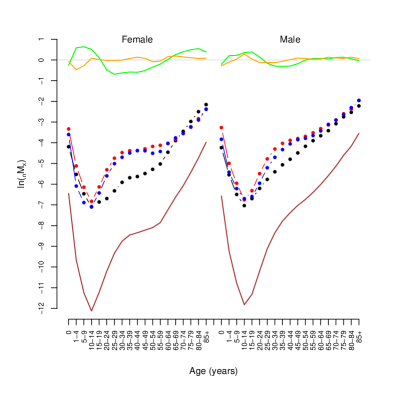
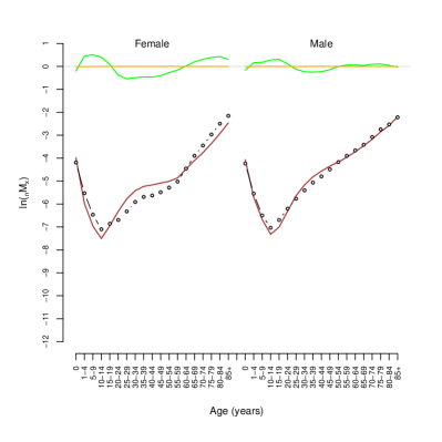
C: Reconstruction of Schedule 2	D: Reconstruction of Schedule 3

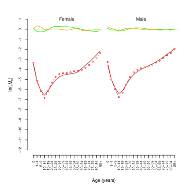
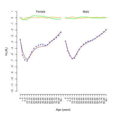
Figure 6: Three-dimension Example with Log Mortality Schedules from Agincourt – Reconstructions. The mortality schedules cover periods 1: 1992-97, 2: 1998-06, and 3: 2007-12; data are in Table A.6. Panel (A): Three-dimension example components $\tensor[_{3}]{\mathbf{\Lambda}}{{}_{i}}\ i\in\{1,2,3\}$; brown = first component $s_{1}\mathbf{u}_{1}$; green = second component $s_{2}\mathbf{u}_{2}$; and orange = third component $s_{3}\mathbf{u}_{3}$. Black dots are data values for mortality schedule 1; red dots are data values for mortality schedule 2; and blue dots are data for mortality schedule 3. Panel (B): Reconstruction of mortality schedule 1; brown = weighted component 1 $v_{11}\tensor[_{3}]{\mathbf{\Lambda}}{{}_{1}}$; green = weighted second component $v_{12}\tensor[_{3}]{\mathbf{\Lambda}}{{}_{2}}$; and orange = weighted third component $v_{13}\tensor[_{3}]{\mathbf{\Lambda}}{{}_{3}}$. Black dots are data values for mortality schedule 1, and white x’s are reconstructed values (all at the center of the data dots) – the sum of weighted components 1–3. Panels (C–D): Same as Panel (B) for mortality schedules 2–3. Notice that the the second (green) component creates the HIV-related ‘hump’ by subtracting it from the primary component for the first period (Panel (A)) and adding small amounts for the other two periods.

A: Mortality Schedule 1 (1992-97)	B: Mortality Schedule 2 (1998-06)
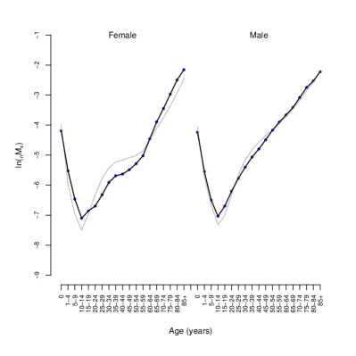
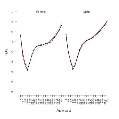
C: Mortality Schedule 3 (2007-12)	C – Weights

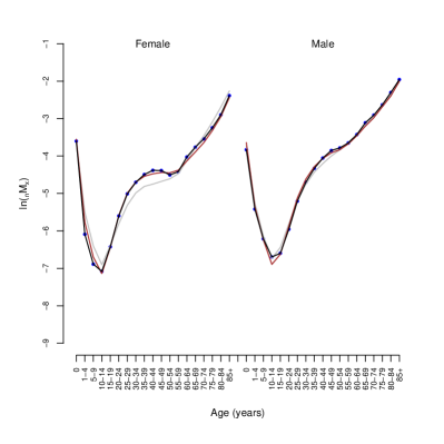
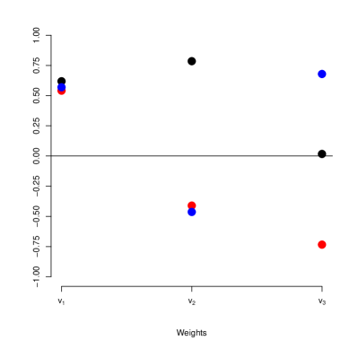
Figure 7: Three-dimension Example with Log Mortality Schedules from Agincourt – Dimension Reduction. The mortality schedules cover periods 1: 1992-97, 2: 1998-06, and 3: 2007-12; data are in Table A.6. Panel (A): Reconstruction of mortality schedule 1 using 1 (grey), 2 (brown) and 3 (black) components. Blue dots are data values. Panels (B–C): Similar reconstructions for mortality schedules 2–3. Notice that reconstructions with the first component (grey) capture the basic shape of the schedules; adding the second component (brown) produces schedules that are very close to the data (or match the data as for the first period), and adding the third component (black) matches the data perfectly. Panel (D): The weights applied to each component to reconstruct the original values. Black is period 1, red is period 2, and blue is period 3. Notice that each period contains a unique ‘pattern’ of weights.

4.2.3 Parameters as Functions of Covariates – Predicting Age Schedules

If there is a systematic relationship between age schedules and an interesting covariate, then Equation 11 indicates that the relationship will also hold between the $\tensor[_{A}]{\beta}{{}_{i}},\ i\in\left\{1\ldots c\right\}$ (hereafter $\tensor[_{A}]{\beta}{{}_{i}^{\prime}}$) and the covariate. Quantifying the relationship between the covariate(s) and the $\tensor[_{A}]{\beta}{{}_{i}^{\prime}}$ allows the $\tensor[_{A}]{\beta}{{}_{i}^{\prime}}$ to be predicted from the covariate, and then the age schedule from the resulting $\tensor[_{A}]{\beta}{{}_{i}^{\prime}}$. This is an efficient way to characterize the relationship between whole age schedules and interesting covariates, and perhaps more usefully, to be able to predict whole age schedules from covariates, even just one. We have applied this idea to an earlier version of the component model of mortality in the context of HIV-related mortality (Sharrow et al., 2014). We will demonstrate it in several examples with both mortality and fertility below.

4.2.4 Identifying Clusters in Collections of Empirical Age Schedules

Now we turn again to the cloud of points associated with a matrix $\mathbf{A}$ of age schedules. As we mentioned above, if there are groups of age schedules in $\mathbf{A}$ that are similar to each other and largely different from the other age schedules in $\mathbf{A}$, then there will be clusters of points in the cloud defined by $\mathbf{A}$. Because of the strong age dependence of all of the age schedules, geometrically these clusters will all be ‘long and thin’, lying close and roughly parallel to a line through the origin and the center of the cloud. Even if we could visualize things in 4+ dimensions, it would be hard to identify and separate these clusters.

The SVD of $\mathbf{A}$ helps solve this problem. Just as the calculated weights did just above when we were thinking about predicting age schedules from covariates, the first few age-schedule- ($h$) and component- ($i$) specific weights $v_{hi}$ in Equation 23 capture most of information necessary to define each individual age schedule in $\mathbf{A}$, and moreover, they quantify the contribution of orthogonal components to each age schedule. Together these properties make them ideal inputs to clustering algorithms such as Mclust (Fraley and Raftery, 2002, 2009) that automatically identify clusters and label their members. We demonstrate this below.

5 Examples

5.1 Example Data: The Agincourt HDSS, South Africa

The models we develop below will be demonstrated using mortality and fertility data from the Agincourt HDSS in South Africa. The Agincourt HDSS has monitored roughly 90,000 people for 22 years between 1992 and the present Kahn et al. (2012). The entire population of the study area is included in the study, and each household is visited annually to update records on vital events, migrations and a variety of other topics. These records allow us to categorize aggregate observed person-time at risk of death and the counts of births and deaths by time, sex and age, and in the case of births, age of the mother as well. This allows us to calculate age-specific event-exposure rates for mortality and fertility through time. Tables A.6, B.7, B.8, C.9 and C.10 in appendices A – C contain the data used in the examples, and Figure 8 displays the data. The purpose of the examples is to illustrate and demonstrate the structure and various uses of the general model, not to extract substantive conclusions about the age-profiles of mortality and fertility at Agincourt. In keeping with that aim, the data have been smoothed in both time and age in order to remove distracting stochastic features and to prevent any meaningful substantive interpretation. The time-sex-age-specific counts of deaths, births and all/female person years were smoothed in both age and time using a customized kernel smoother. The Agincourt data were chosen for this purpose because over the past fifteen years mortality has changed dramatically in response to the HIV epidemic in South Africa and this has produced a series of unusual and often difficult-to-model age patterns of mortality. There is a publicly available version of the Agincourt mortality and fertility data available from the INDEPTH Network public data repositories (http://www.indepth-ishare.org/ and http://www.indepth-ishare.org/indepthstats/).

A: Mortality Rates	B: Fertility Rates

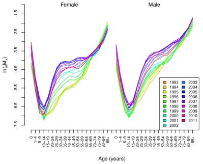
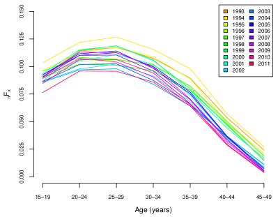
Figure 8: Example Data from Agincourt. (A): Single-year, age-specific log mortality from 1993–2011. These data have been smoothed to make demonstration of the method easier to follow and understand. The counts of births and female person years used to calculate these rates were smoothed in both age and time using a kernel smoother. (B): Single-year, age-specific fertility from 1993–2011. These data have been smoothed to make demonstration of the method easier to follow and understand. The counts of births and person-years used to calculate these rates were smoothed in both age and time using a kernel smoother.

5.2 Component Model for Mortality

In this and following Sections 5.2 – 5.2.1 we define and demonstrate a component model of mortality. We use the example mortality data listed in Tables B.7 and B.8 and displayed in Figure 8. The data consist of annual female and male age-specific mortality rates for ages 0, 1–4, 5–9, 10–14, $\ldots$, 85+ for years 1993–2011. We take the log of these mortality rates and concatenate the female and male age schedules for each year into a single 38-element vector. This is done to ensure that time-specific features of mortality are coupled for females and males. The data also contain covariates: HIV prevalence (% of population), ART Coverage (% of population), expectation of life at birth (years), adult mortality $\tensor[_{45}]{q}{{}_{15}}$, and child mortality $\tensor[_{5}]{q}{{}_{0}}$. Using the component model for mortality, we are able to predict mortality age schedules using these covariates.

The component model of mortality follows the general SVD-based component model in Equation 11. For these example data we calculate the SVD of the $38\times 19$ matrix $\mathbf{AM}$ of concatenated female-male log mortality rates (38 sex-age groups and 19 calendar years). Following the description of the general model in Section 4.2.2, we use the left singular vectors and singular values to construct mortality components $\tensor[_{\text{AM}}]{\mathbf{\Lambda}}{{}_{i}}=\tensor[_{\text{AM}}]{s}{{}_{i}}\cdot\tensor[_{\text{AM}}]{\mathbf{u}}{{}_{i}}$. The first four singular values $\tensor[_{\text{AM}}]{s}{{}_{i}}\ ,\ i\in\{1,2,3,4\}$ are 123.8, 5.1, 1.7, and 1.2, with the remaining singular values $<1.1$. Consequently the new dimensions associated with the first four right singular vectors account for 99.8%, 0.2%, 0.02%, and 0.009% respectively of the total sum of squared perpendicular distances to all of the 38 points in the data set (see Section 3.1). This indicates that the first two new dimensions effectively account for all of the variation in the original data (the remaining variation is lost in rounding error when presenting the results with a readable number of significant figures). Consequently we adopt the following dimension-reduced model with two components,

$$\tensor[_{\text{AM}}]{\widehat{\mathbf{m}}}{{}_{t}} =\sum_{i=1}^{2}\tensor[_{\text{AM}}]{\beta}{{}_{i,t}}\cdot\tensor[_{\text{AM}}]{\mathbf{\Lambda}}{{}_{i}}\ ,$$ (25)

$$\tensor[]{\mathbf{m}}{{}_{t}} =\tensor[_{\text{AM}}]{\widehat{\mathbf{m}}}{{}_{t}}+\tensor[_{\text{AM}}]{\mathbf{r}}{{}_{t}}\ .$$

where $\tensor[_{\text{AM}}]{\widehat{\mathbf{m}}}{{}_{t}}$ is the predicted sex-age mortality schedule for year $t$; $\tensor[_{\text{AM}}]{\beta}{{}_{i,t}}$ are the weights applied to the first two components $\tensor[_{\text{AM}}]{\mathbf{\Lambda}}{{}_{i}}$ (left singular vectors scaled by their corresponding singular values); and $\tensor[_{\text{AM}}]{\mathbf{r}}{{}_{t}}$ is the difference between the predicted and ‘real’ sex-age mortality schedule, possible to calculate when $t$ is one of the years included in the $\mathbf{AM}$ but otherwise an unknown residual when the model is used to predict a mortality schedule not included in $\mathbf{AM}$. Equation 25 is a two-parameter model for sex-age schedules of mortality covering the years 1993–2011. The two components $\tensor[_{\text{AM}}]{\mathbf{\Lambda}}{{}_{i}}\ ,\ i\in\{1,2\}$ are plotted in Figure 9.

The result of predicting the annual mortality schedules using Equation 25 and the first and second weights from the SVD of $\mathbf{AM}$ (the right singular vector weights as in Equation 23) are displayed in Figures D.18 – D.21 in Appendix D. The fits are very close; the total mean absolute error (MAE) is 0.080 ($|\widehat{m}-m|$ across both sexes and all years), and the five-number summary of the distribution of absolute errors is (0.0013, 0.0322, 0.0651, 0.1100, 0.3000), Table 3. The predictions are compared to the real values in a scatterplot in Figure 14, Panel A.

Knowing what we do about the SVD applied to demographic quantities correlated by age, this is not surprising. The real value in our model is the ability to interpolate and extrapolate, and we demonstrate that in the next section using various covariates.

A: Mortality	B: Fertility

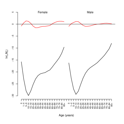
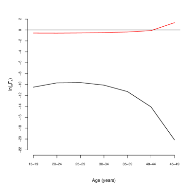
Figure 9: Two Components of the Dimension-reduced Models of Mortality and Fertility at Agincourt. Panel (A): Mortality components. The black line is the first component – the scaled first left singular vector $\tensor[_{\text{AM}}]{\mathbf{\Lambda}}{{}_{1}}$ from the SVD decomposition of Agincourt log mortality rates. The red line is the second component – the scaled second left singular vector $\tensor[_{\text{AM}}]{\mathbf{\Lambda}}{{}_{2}}$. Notice that the first component is well below the x-axis, reflecting the fact that it ‘locates’ the cloud of mortality points. The second component crosses the x-axis because it fine-tunes the location of the mortality points within the cloud. Panel (B): Fertility components. Same as Panel (A) for log fertility rates.

5.2.1 Mortality Age Schedule Covariates and Predictors

As described in Section 4.2.3, a useful feature of the component model is the ability to relate covariates to age schedules through the weights. The basic idea is to model the weights in terms of the covariates and then use that relationship to predict the weights and hence the age schedules. Here we demonstrate this capability with the covariates listed in Tables B.7 and B.8. Life expectancy $\tensor[^{0}]{e}{}$ is a measure of overall level of mortality, HIV prevalence is the fraction of the population infected, ART coverage is the fraction of the population receiving antiretroviral therapy, child mortality $\tensor[_{5}]{q}{{}_{0}}$ is the probability of dying between birth and age 5, and adult mortality $\tensor[_{45}]{q}{{}_{15}}$ is the probability of dying between ages 15 and 60, conditional on surviving to age 15. The fraction of the population that is HIV${{}^{\text{+}}}$ but not on ART is the group of people who die as a result of HIV and is referred to as $\Delta=(\text{HIV prevalence}-\text{ART coverage})$ from now on.

First we have a look at the weights associated with each age schedule that emerge from the SVD of the mortality schedules. In our two-dimension model, these are the first two right singular vectors $\mathbf{v}_{i}\ ,\ i\in\{1,2\}$ ($\mathbf{v}_{1}$ for the first component and $\mathbf{v}_{2}$ for the second component), displayed by year in Figure 10. Figure 11 displays the time trends in $\tensor[^{0}]{e}{}$ and $\Delta$. It is clear that both $\mathbf{v}_{1}$ and $\mathbf{v}_{2}$ are strongly related $\tensor[^{0}]{e}{}$ in a positive, linear sense and related to $\Delta$ in a negative linear sense. These relationships are displayed in Figures 12 and 13 which confirm that they are both approximately linear. Based on this we used OLS regression to estimate two linear models that relate the $\mathbf{v}$’s to the covariates through time $t$,

$$\mathbf{v}_{1,t} =\tensor[_{v1}]{c}{}+\tensor[_{v1}]{\beta}{{}_{1}}\tensor[^{0}]{e}{}_{t}+\tensor[_{v1}]{\beta}{{}_{2}}\Delta_{t}+\tensor[_{v1}]{\epsilon}{{}_{t}}\ ,\phantom{.}$$ (26)

$$\mathbf{v}_{2,t} =\tensor[_{v2}]{c}{}+\tensor[_{v2}]{\beta}{{}_{1}}\tensor[^{0}]{e}{}_{t}+\tensor[_{v2}]{\beta}{{}_{2}}\Delta_{t}+\tensor[_{v2}]{\epsilon}{{}_{t}}\ .$$ (27)

The estimates are displayed in Tables 1 and 2.

Table 1: Estimates for Equation 26: $R^{2}=0.9961$

	Estimate	Std. Error	t value	Pr($>$$|$t$|$)
$\tensor[_{v1}]{c}{}$	0.1024	0.0056	18.26	0.0000
$\tensor[_{v1}]{\beta}{{}_{1}}$	0.0021	0.0001	29.73	0.0000
$\tensor[_{v1}]{\beta}{{}_{2}}$	-0.0005	0.0001	-5.09	0.0001

Table 2: Estimates for Equation 27: $R^{2}=0.9779$

	Estimate	Std. Error	t value	Pr($>$$|$t$|$)
$\tensor[_{v2}]{c}{}$	-0.8532	0.2046	-4.17	0.0007
$\tensor[_{v2}]{\beta}{{}_{1}}$	0.0192	0.0026	7.29	0.0000
$\tensor[_{v2}]{\beta}{{}_{2}}$	-0.0253	0.0034	-7.53	0.0000

Figure 10: Right Singular Vectors of Agincourt Log Mortality Rates by Year. First and second right singular vectors $v_{1}$ and $v_{2}$.

Figure 11: Agincourt Life Expectancy at Birth $\tensor[^{0}]{e}{}$ and Prevalence of Persons Who are HIV⁺ and Not on ART $\Delta$ by Year.

Figure 12: Agincourt Age-specific Log Mortality Rate Right Singular Vectors $\mathbf{v}_{1}$ and $\mathbf{v}_{2}$ by Life Expectancy at Birth $\tensor[^{0}]{e}{}$.

Figure 13: Agincourt Age-specific Log Mortality Rate Right Singular Vectors $\mathbf{v}_{1}$ and $\mathbf{v}_{2}$ by Prevalence of Persons Who are HIV⁺ and Not on ART $\Delta$.

These estimates can now be substituted into Equations 26 and 27 to create expressions that predict the $\mathbf{v}$’s given values for $\tensor[^{0}]{e}{}$ and $\Delta$,

$$\widehat{\mathbf{v}}_{1,t} =\phantom{-}0.1024+0.0021\cdot\tensor[^{0}]{e}{}_{t}-0.0005\cdot\Delta_{t}\ ,$$ (28)

$$\widehat{\mathbf{v}}_{2,t} =-0.8532+0.0192\cdot\tensor[^{0}]{e}{}_{t}-0.0253\cdot\Delta_{t}\ ,$$ (29)

and these predicted $\mathbf{v}$’s can in turn be substituted back into Equation 25 to produce predicted sex-age schedules of mortality, net of the error $\mathbf{r}$. The results of doing this are plotted in Figures B.22 through B.25 in Appendix B. As the figures make clear, the predicted values are very close to the real values. The total MAE (calculated as before) for the predicted values is 0.083, and the five-number summary is (0.0022, 0.0312, 0.0697, 0.1169, 0.2990), Table 3 and Panel (F) of Figure 14.

Table 3: ‘Five Number’ Quantiles of the Distributions of Absolute Prediction Errors for Log Sex-Age-Specific Agincourt Mortality.

Predictor(s)	1%	25%	50%	75%	99%
SVD	0.001311	0.032202	0.065119	0.110022	0.299972
$\tensor[^{0}]{e}{}$ & $\Delta$	0.002174	0.031208	0.069663	0.116879	0.299046
$\tensor[_{5}]{q}{{}_{0}}$	0.002252	0.043255	0.091623	0.152007	0.449184
$\tensor[_{45}]{q}{{}_{15}}$	0.001827	0.035096	0.075179	0.133854	0.354826
$\tensor[_{5}]{q}{{}_{0}}$ & $\tensor[_{45}]{q}{{}_{15}}$	0.002496	0.033556	0.070406	0.131788	0.324306

A similar exercise was conducted to predict sex-age schedules of mortality using child mortality $\tensor[_{5}]{q}{{}_{0}}$ alone, adult mortality $\tensor[_{45}]{q}{{}_{15}}$ alone and child and adult mortality together. The predictions are displayed in Figures B.26 – B.37, and the predictions and their errors are characterized in scatterplots in Figure 14. Similar to the predictions discussed already, in all cases the predictions are very close to the real values. The distributions of absolute errors are described in Table 3 and Panel (F) of Figure 14. The distributions are similar with medians around 0.065 and interquartile ranges around 0.85, except for child mortality which is only slightly worse. This makes sense because child mortality covers only five years at one end of the age schedule and therefore does not contain as much information as the other predictors; nonetheless, it still does well.

A: SVD	B: $\tensor[^{0}]{e}{}$ & $\Delta$	C: $\tensor[_{5}]{q}{{}_{0}}$
D: $\tensor[_{45}]{q}{{}_{15}}$	E: $\tensor[_{5}]{q}{{}_{0}}$ & $\tensor[_{45}]{q}{{}_{15}}$	F

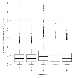
Figure 14: Prediction Error in Agincourt Log Mortality Schedules: Scatterplots of Predictions vs. Data. Each point in the scatterplots is a pair of time-sex-age-specific log mortality rates, 38 sex-age groups $\times$ 19 years = 722 points per plot. Panel (A): Weights from the right singular vectors of the SVD of $\mathbf{AM}$. Panel (B): Weights predicted from $\tensor[^{0}]{e}{}$ and $\Delta$. Panel (C): Weights predicted from child mortality $\tensor[_{5}]{q}{{}_{0}}$. Panel (D): Weights predicted from adult mortality $\tensor[_{45}]{q}{{}_{15}}$. Panel (E): Weights predicted from child $\tensor[_{5}]{q}{{}_{0}}$ and adult $\tensor[_{45}]{q}{{}_{15}}$ mortality. Panel (F): Boxplots of distributions of absolute error in predictions of Agincourt log Mortality. The letters on the horizontal axis correspond, in order, to the panels of this figure.

5.2.2 Identifying ‘Common’ Age Schedules of Mortality

The sequence or ‘pattern’ of weights applied to the first few components in a SVD-based component model contain the information necessary to reconstruct the original data to within a level of precision related to the number of components used in the model. Treating the components as fixed parameters, the weights themselves contain all the information. As described in Section 4.2.4 and illustrated in Figure 7, it is possible to use the information contained in the weights to identify similar age schedules, and hence groups of similar age schedules.

We briefly demonstrate this potential using the log Agincourt mortality schedules discussed above in Sections 5.2 and 5.2.1. We examine the first two right singular vectors of the SVD of $\mathbf{AM}$ which contain the weights used to reconstruct the rank-2 version of $\mathbf{AM}$. Treating these as a two-dimensional, compact representation of the age schedules contained in $\mathbf{AM}$, we use the model-based clustering algorithm Mclust (Fraley and Raftery, 2002, 2009) to identify clusters of similar row vectors in the matrix formed by the first two right singular vectors,

$$\left[\begin{matrix}|&|\\ \mathbf{v}_{1}&\mathbf{v}_{2}\\ |&|\end{matrix}\right].$$ (30)

Mclust simultaneously identifies the optimal number of clusters and classifies each row of the dataset into one of the clusters. Applied to the nineteen Agincourt mortality schedules, Mclust identified four clusters – 1: 1993–1997, 2: 1998–2002, 3: 2003–2008, and 4: 2009-2011. Within each of these clusters, we calculated the median values of $\mathbf{v}_{1}$ and $\mathbf{v}_{2}$ and reconstructed the log mortality age schedules for each cluster using those median values, displayed in Figure 15. These form the ‘characteristic’ smoothed (reduced-dimension) age patterns for each of the periods identified by Mclust.

Theses periods are substantively sensible – 1: pre-HIV (no hump, generally low mortality), 2: developing HIV epidemic and no ART (hump developing and child mortality increasing), 3: height of HIV epidemic and beginning of sporadic roll-out of ART (very pronounced effects of HIV), and 4: ART available, coverage continuing to increase and mortality-reduction effects of ART beginning to be felt (attenuation of HIV-related mortality).

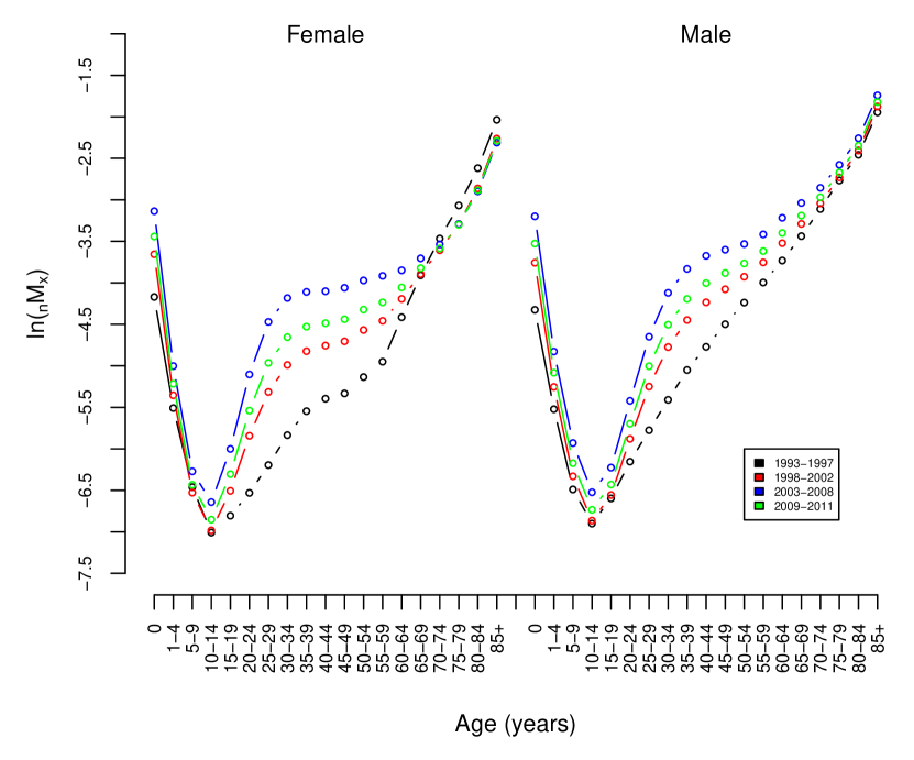
Figure 15: Four Characteristic Age Patterns of Agincourt Log Mortality Rates. The Mclust clustering method was used to identify four groups of similar weights on the two components retained in the reduced dimension model of Agincourt mortality. The model patterns generated using the median weights for each group are 1: 1993–1997, 2: 1998–2002, 3: 2003–2008, and 4: 2009–2011.

5.3 Component Model for Fertility

In this and following Sections 5.3 – 5.3.1 we define and demonstrate a component model of fertility, following the same general procedure as we employed for mortality in Sections 5.2 – 5.2.1. We use the example mortality data listed in Tables C.9 and C.10 and displayed in Figure 8. The data consist of annual age-specific fertility rates for ages 15–19, 20-24, $\ldots$, 45-49 for years 1993–2011. In what follows we work with the log fertility rates. The data also contain one covariate, the total fertility rate (TFR). Using the component model for mortality, we predict fertility age schedules using the TFR.

As with mortality, the component model of fertility follows the general SVD-based component model in Equation 11. We calculate the SVD of the $7\times 19$ matrix $\mathbf{AF}$ of log fertility rates. Following the description of the general model in Section 4.2.2, we use the left singular vectors and singular values to construct fertility components $\tensor[_{\text{AF}}]{\mathbf{\Lambda}}{{}_{i}}=\tensor[_{\text{AF}}]{s}{{}_{i}}\cdot\tensor[_{\text{AF}}]{\mathbf{u}}{{}_{i}}$. The first four singular values $\tensor[_{\text{AF}}]{s}{{}_{i}}\ ,\ i\in\{1,2,3,4\}$ are 33.64, 1.76, 0.22, and 0.18, with the remaining singular values $<0.13$. Consequently the new dimensions associated with the first four right singular vectors account for 99.7%, 0.3%, 0.004%, and 0.003% respectively of the total sum of squared perpendicular distances to all of the 7 points in the data set (see Section 3.1). This indicates that the first two new dimensions effectively account for all of the variation in the original data (the remaining variation is lost in rounding error when presenting the results with a readable number of significant figures). Consequently we adopt the following dimension-reduced model with two components,

$$\tensor[_{\text{AF}}]{\widehat{\mathbf{f}}}{{}_{t}} =\sum_{i=1}^{2}\tensor[_{\text{AF}}]{\beta}{{}_{i,t}}\cdot\tensor[_{\text{AF}}]{\mathbf{\Lambda}}{{}_{i}}\ ,$$ (31)

$$\tensor[]{\mathbf{f}}{{}_{t}} =\tensor[_{\text{AF}}]{\widehat{\mathbf{f}}}{{}_{t}}+\tensor[_{\text{AF}}]{\mathbf{r}}{{}_{t}}\ .$$

where $\tensor[_{\text{AF}}]{\widehat{\mathbf{f}}}{{}_{t}}$ is the predicted age-specific fertility schedule for year $t$; $\tensor[_{\text{AF}}]{\beta}{{}_{i,t}}$ are the weights applied to the first two components $\tensor[_{\text{AF}}]{\mathbf{\Lambda}}{{}_{i}}$ (left singular vectors scaled by their corresponding singular values); and $\tensor[_{\text{AF}}]{\mathbf{r}}{{}_{t}}$ is the difference between the predicted and ‘real’ age-specific fertility schedule, possible to calculate when $t$ is one of the years included in the $\mathbf{AF}$ but otherwise an unknown residual when the model is used to predict a mortality schedule not included in $\mathbf{AF}$. Equation 31 is a two-parameter model for age-specific schedules of fertility covering the years 1993–2011. The two components $\tensor[_{\text{AF}}]{\mathbf{\Lambda}}{{}_{i}}\ ,\ i\in\{1,2\}$ are plotted in Figure 9.

5.3.1 Fertility Age Schedule Covariates and Predictors

As we did with mortality, we can construct a model of the weights that predict fertility in Equation 31 using a covariate to predict the weights. For fertility we will use the TFR or overall level as our predictor and see if we can accurately predict the age-pattern of fertility from TFR. The time trend in the TFR is displayed in Figure 16, and the relationship between the TFR and the first two right singular vectors of the SVD of the age-specific fertility rates $\mathbf{AF}$ is displayed in Figure 17. The relationships between the $\mathbf{v}$’s and TFR is linear but less strong than the relationships between the $\mathbf{v}$’s for mortality and their predictors. Nonetheless, we model each with a simple linear equation and estimate the coefficients with OLS. The results are displayed in Tables 4 and 5 with structures exactly analogous to Equations 26 and 27 used for the mortality model above in Section 5.2.1.

Figure 16: Agincourt Total Fertility Rate (TFR) by Year.

Figure 17: Agincourt Age-specific Log Fertility Rate Right Singular Vectors $\mathbf{v}_{1}$ and $\mathbf{v}_{2}$ by Total Fertility Rate (TFR).

Table 4: OLS Estimates for Linear Model of Fertility $\mathbf{v}_{1}$ by TFR: $R^{2}=0.746$

	Estimate	Std. Error	t value	Pr($>$$|$t$|$)
$\tensor[_{v1}]{c}{}$	0.344799	0.016529	20.860334	0.000000
$\tensor[_{v1}]{\beta}{{}_{1}}$	-0.039329	0.005566	-7.065603	0.000002

Table 5: OLS Estimates for Linear Model of Fertility $\mathbf{v}_{2}$ by TFR: $R^{2}=0.431$

	Estimate	Std. Error	t value	Pr($>$$|$t$|$)
$\tensor[_{v2}]{c}{}$	-1.236473	0.350591	-3.526825	0.002589
$\tensor[_{v2}]{\beta}{{}_{1}}$	0.424483	0.118063	3.595388	0.002231

Using these relationships to predict the weights in Equation 31 we predict the age-specific fertility schedules displayed on their natural scale in Figures E.38 to E.41 in Appendix E. The MAE for the prediction errors across age groups and years on the log scale is 0.0834, and the five-number summary is 0.0021, 0.0167, 0.0395, 0.0795, 0.6440. As with mortality the predictions are surprisingly close to the data given the single predictor; this can be verified visually by looking at the Figures in Appendix E.

6 Discussion

The SVD is a classic matrix decomposition that factorizes an arbitrary matrix into three new matrices with useful properties. The right singular vectors $\mathbf{V}$ identify a new orthonormal basis for the row vectors or points in the original matrix; the singular values correspond to how much variation among the points in the original matrix is captured by each of the new dimensions; and for each point, the left singular vectors $\mathbf{U}$ stretch or shrink the new dimensions, scaled by their singular values, into a set of vectors whose sum locates the original points.

The SVD can be reorganized into a different form – the Eckart-Young-Mirsky formula – that expresses the original matrix as a sum or rank-1 matrices, and it has been shown that truncated sums of these rank-1 matrices represent the best reduced-rank approximations of the origin matrix in a perpendicular least squares sense. An intermediate step on the way to deriving the EYM formula expresses each column vector in the original matrix as a weighted sum of the left singular vectors scaled by their singular values, with the weights being the right singular vectors. Because they are equivalent to the EYM form, these weighted sums have the property that the first few terms contain the vast majority of the information necessary to represent the columns in the original matrix. This allows each column in the original matrix to be closely approximated by a weighted sum with potentially very few terms. Not including the remaining terms also eliminates ‘noise’, i.e. small magnitude variation that is not age-specific, and this provides a principled means by which to smooth the columns in the original matrix.

The SVD can be applied directly to age schedules of quantities that are correlated by age because data with that property are always arranged in a multidimensional cloud whose primary axis or dimension is very close to a line that intersects the origin. This ensures that the first right singular vector derived from an SVD of these data is approximately lined up with the primary dimension of the cloud, and this in turn provides a standard interpretation of the first new dimension $\mathbf{v}_{1}$ and more importantly the first left singular vector $\mathbf{u}_{1}$. $\mathbf{u}_{1}$ for a set of points correlated by age is the principal shape of the age schedule with age, and the remaining $\mathbf{u}$’s are age-specific deviations on that main shape, and typically only the first few represent systematic age-specific deviations, with the rest effectively being noise.

Combining our understanding of the SVD and the fact that the SVD of demographic quantitates correlated by age behaves in a predictable and interpretable way, we propose a general ‘component model’ of demographic quantitates correlated by age. This model given in Equation 11 represents an arbitrary age schedule as the weighted sum of components derived from the SVD of a matrix of similar age schedules. The weights can come from the SVD that is used to define the components (if one wants to reconstruct or smooth the original data matrix) or by estimating an OLS linear regression model of an arbitrary age schedule as a function of the components, with no intercept. The model can be used for a variety of purposes including:

• to smooth age schedules;

• to (dramatically) reduce the amount of information necessary to represent a large number of age schedules;

• to represent a single age schedule with a small number of weights, typically 2–3, by treating the components as fixed parameters;

• to predict new age schedules by supplying values for the weights, and

• to cluster age schedules by applying a clustering algorithm to the weights.

A particularly useful application of the component model is to use it to represent age schedules as a function of arbitrary predictors or covariates. This is done by modeling the right singular vectors of the SVD used to create the components as functions of the predictors. These models can be used to predict the weights using values supplied for the predictors/covariates, and the predicted weights can then be used to predict the age schedules. This is a simple and general way to relate covariates to whole age structures and likely has many applications.

We demonstrate all of these properties and uses of the component model using example data from the Agincourt HDSS site in rural South Africa. The component model is able to accurately reconstruct age-specific mortality and fertility rates starting with the original SVD-derived weights and/or weights predicted using simple models of the observed relationships between weights and covariates.

Appendix A Example Data

Table 6: Example Mortality Rates: Agincourt Smoothed and Aggregated into Three Periods (Kahn et al., 2012).

Sex	Age Group	1992–1997	1998–2006	2007–2012
Female	0	0.01514	0.03575	0.02730
Female	1-4	0.00398	0.00598	0.00227
Female	5-9	0.00156	0.00214	0.00102
Female	10-14	0.00082	0.00108	0.00084
Female	15-19	0.00105	0.00217	0.00162
Female	20-24	0.00124	0.00497	0.00370
Female	25-29	0.00180	0.00869	0.00667
Female	30-34	0.00271	0.01140	0.00909
Female	35-39	0.00339	0.01246	0.01117
Female	40-44	0.00359	0.01264	0.01249
Female	45-49	0.00414	0.01364	0.01244
Female	50-54	0.00508	0.01536	0.01104
Female	55-59	0.00658	0.01619	0.01206
Female	60-64	0.01161	0.01755	0.01784
Female	65-69	0.02032	0.02174	0.02320
Female	70-74	0.03176	0.02853	0.02896
Female	75-79	0.05130	0.03989	0.03894
Female	80-84	0.08233	0.05865	0.05500
Female	85+	0.11596	0.09346	0.09200
Male	0	0.01447	0.03821	0.02170
Male	1-4	0.00390	0.00678	0.00443
Male	5-9	0.00151	0.00259	0.00200
Male	10-14	0.00088	0.00117	0.00124
Male	15-19	0.00124	0.00181	0.00137
Male	20-24	0.00202	0.00413	0.00259
Male	25-29	0.00312	0.00842	0.00549
Male	30-34	0.00451	0.01356	0.00908
Male	35-39	0.00631	0.01777	0.01318
Male	40-44	0.00827	0.02061	0.01735
Male	45-49	0.01122	0.02250	0.02124
Male	50-54	0.01543	0.02492	0.02273
Male	55-59	0.02025	0.02966	0.02600
Male	60-64	0.02570	0.03621	0.03248
Male	65-69	0.03285	0.04325	0.04452
Male	70-74	0.04600	0.05516	0.05463
Male	75-79	0.06416	0.07414	0.07191
Male	80-84	0.07973	0.09298	0.09995
Male	85+	0.10870	0.14229	0.14114

Appendix B Smoothed Agincourt Mortality Rates

Table 7: Agincourt Mortality Rates: Smoothed 1993–2002 (Kahn et al., 2012).

	Indicator
Sex	Age Group	1993	1994	1995	1996	1997	1998	1999	2000	2001	2002
Both	HIV Prevalencea	0.03243	0.04624	0.06366	0.08401	0.10568	0.12657	0.14476	0.15909	0.16938	0.17607
Both	ART Coverageb	0.00000	0.00000	0.00000	0.00000	0.00000	0.00000	0.00000	0.00000	0.00013	0.00030
Both	$\tensor[^{0}]{e}{}$	70.13	69.32	68.44	69.55	69.40	68.79	66.39	64.00	62.34	59.03
Both	$\tensor[_{45}]{q}{{}_{15}}$	0.21467	0.22811	0.23932	0.23759	0.24640	0.26771	0.28508	0.31503	0.35818	0.42472
Both	$\tensor[_{5}]{q}{{}_{0}}$	0.03066	0.03003	0.02982	0.02760	0.02748	0.03262	0.04829	0.05393	0.05486	0.05997
Female	0	0.01537	0.01529	0.01606	0.01548	0.01342	0.01598	0.02893	0.03203	0.03214	0.03398
Female	1-4	0.00414	0.00409	0.00387	0.00329	0.00379	0.00426	0.00535	0.00568	0.00595	0.00674
Female	5-9	0.00179	0.00149	0.00143	0.00116	0.00148	0.00149	0.00168	0.00156	0.00182	0.00217
Female	10-14	0.00097	0.00098	0.00083	0.00092	0.00082	0.00072	0.00078	0.00079	0.00108	0.00125
Female	15-19	0.00099	0.00100	0.00102	0.00106	0.00103	0.00145	0.00146	0.00162	0.00193	0.00241
Female	20-24	0.00115	0.00126	0.00130	0.00132	0.00179	0.00244	0.00294	0.00376	0.00388	0.00493
Female	25-29	0.00172	0.00191	0.00209	0.00193	0.00242	0.00332	0.00386	0.00527	0.00648	0.00825
Female	30-34	0.00281	0.00309	0.00314	0.00273	0.00288	0.00416	0.00527	0.00712	0.00815	0.01021
Female	35-39	0.00378	0.00399	0.00403	0.00351	0.00394	0.00537	0.00640	0.00882	0.00952	0.01146
Female	40-44	0.00391	0.00468	0.00470	0.00422	0.00420	0.00640	0.00784	0.00987	0.01004	0.01217
Female	45-49	0.00479	0.00526	0.00475	0.00421	0.00493	0.00631	0.00731	0.00893	0.01089	0.01336
Female	50-54	0.00610	0.00639	0.00624	0.00550	0.00591	0.00675	0.00764	0.00980	0.01251	0.01477
Female	55-59	0.00700	0.00675	0.00676	0.00722	0.00802	0.00788	0.00964	0.01073	0.01410	0.01583
Female	60-64	0.00967	0.01138	0.01134	0.01213	0.01504	0.01264	0.01457	0.01578	0.01750	0.01786
Female	65-69	0.01843	0.01899	0.01979	0.01975	0.02022	0.01845	0.02054	0.01993	0.02229	0.02231
Female	70-74	0.02871	0.03111	0.03030	0.02979	0.03076	0.02781	0.02747	0.02676	0.02906	0.02639
Female	75-79	0.04341	0.04483	0.04643	0.04582	0.04059	0.03822	0.03682	0.04130	0.04300	0.03919
Female	80-84	0.06807	0.07707	0.08109	0.07562	0.06203	0.04711	0.04865	0.06367	0.06609	0.06958
Female	85+	0.12280	0.13903	0.14629	0.13642	0.11190	0.08499	0.08777	0.11485	0.11923	0.12552
Male	0	0.01440	0.01224	0.01295	0.01282	0.01189	0.01573	0.02512	0.02786	0.02860	0.03297
Male	1-4	0.00375	0.00408	0.00380	0.00341	0.00359	0.00418	0.00577	0.00698	0.00700	0.00740
Male	5-9	0.00164	0.00164	0.00155	0.00119	0.00123	0.00138	0.00185	0.00193	0.00194	0.00223
Male	10-14	0.00113	0.00112	0.00100	0.00085	0.00086	0.00083	0.00089	0.00095	0.00097	0.00110
Male	15-19	0.00130	0.00156	0.00141	0.00112	0.00118	0.00129	0.00131	0.00127	0.00152	0.00205
Male	20-24	0.00183	0.00212	0.00208	0.00221	0.00229	0.00241	0.00227	0.00259	0.00325	0.00431
Male	25-29	0.00241	0.00294	0.00312	0.00377	0.00385	0.00416	0.00426	0.00451	0.00563	0.00780
Male	30-34	0.00359	0.00415	0.00416	0.00546	0.00597	0.00664	0.00686	0.00762	0.00872	0.01196
Male	35-39	0.00535	0.00616	0.00632	0.00741	0.00802	0.00900	0.00964	0.01040	0.01164	0.01531
Male	40-44	0.00704	0.00833	0.00872	0.00985	0.00984	0.01079	0.01185	0.01256	0.01434	0.01771
Male	45-49	0.00938	0.01071	0.01215	0.01284	0.01239	0.01315	0.01399	0.01456	0.01577	0.01926
Male	50-54	0.01304	0.01473	0.01668	0.01558	0.01610	0.01603	0.01527	0.01454	0.01715	0.02213
Male	55-59	0.02051	0.01895	0.02197	0.01960	0.01908	0.01722	0.01591	0.01622	0.02100	0.02761
Male	60-64	0.02670	0.02448	0.03044	0.02405	0.02443	0.02129	0.02074	0.02093	0.02641	0.03407
Male	65-69	0.03098	0.03070	0.03925	0.03037	0.03356	0.03210	0.03251	0.03297	0.03400	0.03825
Male	70-74	0.03834	0.04164	0.05165	0.04011	0.04548	0.04520	0.05016	0.05526	0.04691	0.04881
Male	75-79	0.05518	0.06372	0.07056	0.05732	0.06157	0.05930	0.06644	0.07824	0.06387	0.06913
Male	80-84	0.09120	0.08723	0.09655	0.07910	0.06965	0.07560	0.08534	0.09819	0.08729	0.09653
Male	85+	0.15344	0.14676	0.16244	0.13309	0.11719	0.12719	0.14358	0.16520	0.14687	0.16242

• Source: United Nations, Department of Economic and Social Affairs, Population Division, (2011)

• Source: ART coverage is number on ART divided by population. For Mpumalanga Province, numbers on ART through 2008 from Day and Gray (2010), extrapolated through 2011 using observed growth rate in previous years. Population of Mpumalanga Province assumed to be 4M.

Table 8: Agincourt Mortality Rates: Smoothed 2003–2011 (Kahn et al., 2012).

	Indicator
Sex	Age Group	2003	2004	2005	2006	2007	2008	2009	2010	2011
Both	HIV Prevalencea	0.17993	0.18174	0.18218	0.18059	0.17962	0.17870	0.17782	0.17689	0.17586
Both	ART Coverageb	0.00050	0.00077	0.00140	0.00298	0.00575	0.00925	0.01249	0.01661	0.02192
Both	$\tensor[^{0}]{e}{}$	56.09	55.20	54.37	53.83	54.07	54.77	57.98	60.64	62.43
Both	$\tensor[_{45}]{q}{{}_{15}}$	0.47853	0.51034	0.53773	0.54112	0.53425	0.51198	0.45785	0.41664	0.38816
Both	$\tensor[_{5}]{q}{{}_{0}}$	0.06905	0.06710	0.06649	0.06772	0.07102	0.07275	0.05923	0.04653	0.03822
Female	0	0.03691	0.03815	0.03990	0.04646	0.04800	0.04914	0.03873	0.02788	0.02533
Female	1-4	0.00740	0.00654	0.00660	0.00721	0.00740	0.00691	0.00531	0.00406	0.00365
Female	5-9	0.00245	0.00188	0.00161	0.00223	0.00228	0.00192	0.00137	0.00123	0.00104
Female	10-14	0.00148	0.00139	0.00125	0.00144	0.00141	0.00153	0.00102	0.00095	0.00094
Female	15-19	0.00257	0.00250	0.00235	0.00258	0.00227	0.00214	0.00177	0.00174	0.00168
Female	20-24	0.00568	0.00641	0.00572	0.00587	0.00553	0.00489	0.00396	0.00356	0.00353
Female	25-29	0.00944	0.01147	0.01152	0.01207	0.01097	0.00988	0.00811	0.00711	0.00636
Female	30-34	0.01300	0.01581	0.01562	0.01650	0.01530	0.01379	0.01111	0.00976	0.00916
Female	35-39	0.01373	0.01637	0.01715	0.01738	0.01570	0.01462	0.01248	0.01147	0.01127
Female	40-44	0.01440	0.01630	0.01661	0.01668	0.01555	0.01379	0.01216	0.01226	0.01280
Female	45-49	0.01542	0.01671	0.01838	0.01855	0.01702	0.01483	0.01309	0.01200	0.01269
Female	50-54	0.01803	0.01852	0.02010	0.02113	0.02011	0.01771	0.01539	0.01301	0.01150
Female	55-59	0.01764	0.01812	0.01963	0.02153	0.02086	0.01981	0.01784	0.01506	0.01344
Female	60-64	0.02098	0.01980	0.01987	0.02077	0.02037	0.02121	0.01965	0.01912	0.01693
Female	65-69	0.02286	0.02294	0.02310	0.02528	0.02526	0.02440	0.02289	0.02451	0.02433
Female	70-74	0.02585	0.02415	0.02677	0.03120	0.03198	0.03223	0.03101	0.02971	0.03098
Female	75-79	0.03505	0.03214	0.03469	0.03699	0.03734	0.03722	0.04059	0.03889	0.04193
Female	80-84	0.06344	0.05615	0.05265	0.05507	0.05267	0.05169	0.05751	0.05464	0.05652
Female	85+	0.11444	0.10129	0.09497	0.09935	0.09502	0.09324	0.10375	0.09857	0.10197
Male	0	0.04226	0.04270	0.04089	0.03673	0.03934	0.04113	0.03583	0.02827	0.01940
Male	1-4	0.00863	0.00801	0.00763	0.00713	0.00767	0.00839	0.00657	0.00560	0.00453
Male	5-9	0.00272	0.00244	0.00247	0.00247	0.00286	0.00301	0.00242	0.00239	0.00185
Male	10-14	0.00132	0.00139	0.00139	0.00141	0.00161	0.00171	0.00165	0.00168	0.00123
Male	15-19	0.00212	0.00214	0.00195	0.00175	0.00186	0.00214	0.00194	0.00170	0.00143
Male	20-24	0.00477	0.00483	0.00458	0.00434	0.00436	0.00464	0.00337	0.00289	0.00288
Male	25-29	0.00902	0.01015	0.01034	0.01000	0.01007	0.00960	0.00767	0.00603	0.00535
Male	30-34	0.01405	0.01621	0.01728	0.01731	0.01806	0.01673	0.01285	0.01016	0.00909
Male	35-39	0.01795	0.02070	0.02260	0.02332	0.02498	0.02285	0.01884	0.01530	0.01236
Male	40-44	0.02069	0.02300	0.02619	0.02650	0.02851	0.02749	0.02362	0.02034	0.01702
Male	45-49	0.02292	0.02537	0.02935	0.02879	0.02901	0.02831	0.02591	0.02440	0.02067
Male	50-54	0.02584	0.02882	0.03341	0.03238	0.03138	0.03123	0.02785	0.02559	0.02348
Male	55-59	0.03443	0.03373	0.03889	0.03746	0.03778	0.03698	0.03059	0.02627	0.02365
Male	60-64	0.04206	0.04020	0.04585	0.04645	0.04400	0.04552	0.03978	0.03347	0.03030
Male	65-69	0.04638	0.04703	0.04959	0.05239	0.04873	0.05360	0.04851	0.04280	0.04052
Male	70-74	0.05563	0.05532	0.05774	0.06153	0.05235	0.05629	0.05651	0.05320	0.05163
Male	75-79	0.07527	0.07682	0.08076	0.07604	0.07241	0.07094	0.07097	0.06811	0.07070
Male	80-84	0.10541	0.10065	0.10176	0.10799	0.10145	0.10184	0.10565	0.10748	0.10329
Male	85+	0.17734	0.16934	0.17121	0.18170	0.17069	0.17134	0.17776	0.18084	0.17378

• Source: United Nations, Department of Economic and Social Affairs, Population Division, (2011)

• Source: ART coverage is number on ART divided by population. For Mpumalanga Province, numbers on ART through 2008 from Day and Gray (2010), extrapolated through 2011 using observed growth rate in previous years. Population of Mpumalanga Province assumed to be 4M.

Appendix C Smoothed Agincourt Fertility Rates

Table 9: Agincourt Fertility Rates: Smoothed 1993–2002 (Kahn et al., 2012)

Age Group	1993	1994	1995	1996	1997	1998	1999	2000	2001	2002
TFR	3.47	3.71	3.29	3.00	3.31	2.88	3.29	3.18	2.91	2.60
15-19	0.09103	0.10335	0.09637	0.09019	0.09566	0.09008	0.08658	0.09359	0.09184	0.08659
20-24	0.11408	0.12194	0.11281	0.10503	0.10829	0.10209	0.11455	0.11528	0.10543	0.09787
25-29	0.11732	0.12674	0.11740	0.10592	0.10666	0.10126	0.11885	0.11861	0.11079	0.10230
30-34	0.10750	0.11548	0.10892	0.10162	0.10112	0.09623	0.10542	0.10616	0.10208	0.09137
35-39	0.08941	0.09807	0.08883	0.08200	0.08224	0.07847	0.07976	0.07708	0.07370	0.06812
40-44	0.05357	0.05699	0.04891	0.04863	0.05050	0.04751	0.04679	0.04414	0.03583	0.03477
45-49	0.02418	0.02716	0.02118	0.01926	0.01858	0.01471	0.01510	0.01674	0.01084	0.00900

Table 10: Agincourt Fertility Rates: 2003–2011 (Kahn et al., 2012).

Age Group	2003	2004	2005	2006	2007	2008	2009	2010	2011
TFR	2.56	2.61	3.05	3.02	2.77	2.92	2.34	2.56	2.56
15-19	0.08582	0.08639	0.09255	0.09255	0.09026	0.09064	0.08908	0.08470	0.07633
20-24	0.09696	0.10184	0.11163	0.11018	0.11008	0.11308	0.10753	0.10636	0.09588
25-29	0.09794	0.10247	0.11411	0.11254	0.11041	0.11263	0.10416	0.10638	0.09572
30-34	0.08394	0.08733	0.09839	0.10000	0.09587	0.09951	0.09046	0.09415	0.08582
35-39	0.06415	0.06612	0.07522	0.07675	0.06983	0.07046	0.06529	0.06636	0.06421
40-44	0.03675	0.03582	0.03649	0.03678	0.03279	0.03395	0.03124	0.02930	0.02879
45-49	0.01115	0.00788	0.00557	0.00706	0.00515	0.00505	0.00492	0.00422	0.00386

Appendix D Predicted Age-Specific Mortality Plots

Figure 18: Age-specific Log Mortality Rates Predicted using Right Singular Vector Weights, 1993–1998. The red dots are the data, and the solid black line indicates predicted values.

Figure 19: Age-specific Log Mortality Rates Predicted using Right Singular Vector Weights, 1999–2004. The red dots are the data, and the solid black line indicates predicted values.

Figure 20: Age-specific Log Mortality Rates Predicted using Right Singular Vector Weights, 2005–2010. The red dots are the data, and the solid black line indicates predicted values.

Figure 21: Age-specific Log Mortality Rates Predicted using Right Singular Vector Weights, 2011. The red dots are the data, and the solid black line indicates predicted values.

Figure 22: Age-specific Log Mortality Rates Predicted as a Function of Life Expectancy at Birth and Prevalence of Persons Who are HIV⁺ and Not on ART, 1993–1998. The red dots are the data, and the solid black line indicates predicted values.

Figure 23: Age-specific Log Mortality Rates Predicted as a Function of Life Expectancy at Birth and Prevalence of Persons Who are HIV⁺ and Not on ART, 1999–2004. The red dots are the data, and the solid black line indicates predicted values.

Figure 24: Age-specific Log Mortality Rates Predicted as a Function ofLife Expectancy at Birth and Prevalence of Persons Who are HIV⁺ and Not on ART, 2005–2010. The red dots are the data, and the solid black line indicates predicted values.

Figure 25: Age-specific Log Mortality Rates Predicted as a Function of Life Expectancy at Birth and Prevalence of Persons Who are HIV⁺ and Not on ART, 2011. The red dots are the data, and the solid black line indicates predicted values.

Figure 26: Age-specific Log Mortality Rates Predicted as a Function of Child Mortality, 1993–1998. The red dots are the data, and the solid black line indicates predicted values.

Figure 27: Age-specific Log Mortality Rates Predicted as a Function of Child Mortality, 1999–2004. The red dots are the data, and the solid black line indicates predicted values.

Figure 28: Age-specific Log Mortality Rates Predicted as a Function of Child Mortality, 2005–2010. The red dots are the data, and the solid black line indicates predicted values.

Figure 29: Age-specific Log Mortality Rates Predicted as a Function of Child Mortality, 2011. The red dots are the data, and the solid black line indicates predicted values.

Figure 30: Age-specific Log Mortality Rates Predicted as a Function of Adult Mortality, 1993–1998. The red dots are the data, and the solid black line indicates predicted values.

Figure 31: Age-specific Log Mortality Rates Predicted as a Function of Adult Mortality, 1999–2004. The red dots are the data, and the solid black line indicates predicted values.

Figure 32: Age-specific Log Mortality Rates Predicted as a Function of Adult Mortality, 2005–2010. The red dots are the data, and the solid black line indicates predicted values.

Figure 33: Age-specific Log Mortality Rates Predicted as a Function of Adult Mortality, 2011. The red dots are the data, and the solid black line indicates predicted values.

Figure 34: Age-specific Log Mortality Rates Predicted as a Function of Child and Adult Mortality, 1993–1998. The red dots are the data, and the solid black line indicates predicted values.

Figure 35: Age-specific Log Mortality Rates Predicted as a Function of Child and Adult Mortality, 1999–2004. The red dots are the data, and the solid black line indicates predicted values.

Figure 36: Age-specific Log Mortality Rates Predicted as a Function of Child and Adult Mortality, 2005–2010. The red dots are the data, and the solid black line indicates predicted values.

Figure 37: Age-specific Log Mortality Rates Predicted as a Function of Child and Adult Mortality, 2011. The red dots are the data, and the solid black line indicates predicted values.

Appendix E Predicted Age-Specific Fertility Plots

Figure 38: Age-specific Fertility Rates Predicted as a Function of the Total Fertility Rate, 1993–1998. The red dots are the data, and the solid black line indicates predicted values.

Figure 39: Age-specific Fertility Rates Predicted as a Function of the Total Fertility Rate, 1999–2004. The red dots are the data, and the solid black line indicates predicted values.

Figure 40: Age-specific Fertility Rates Predicted as a Function of the Total Fertility Rate, 2005–2010. The red dots are the data, and the solid black line indicates predicted values.

Figure 41: Agincourt Age-specific Fertility Rates Predicted as a Function of the Total Fertility Rate, 2011. The red dots are the data, and the solid black line indicates predicted values.

References

- Abdi and Williams (2010) Abdi, H. and L. J. Williams (2010). Principal component analysis. Wiley Interdisciplinary Reviews: Computational Statistics 2(4), 433–459.
- Clark (2001) Clark, S. J. (2001). An Investigation into the Impact of HIV on Population Dynamics in Africa. Ph.d., University of Pennsylvania.
- Clark et al. (2009) Clark, S. J., M. Jasseh, S. Punpuing, E. Zulu, A. Bawah, and O. Sankoh (2009, May). Indepth model life tables 2.0. In Annual Conference of the Population Association of America (PAA). Population Association of America (PAA).
- Coale and Trussell (1996) Coale, A. and J. Trussell (1996). The development and use of demographic models. Population Studies 50(3), 469–484.
- Coale and Demeny (1966) Coale, A. J. and P. Demeny (1966). Regional Model Life Tables and Stable Populations. Princeton University Press.
- Coale and Trussell (1974) Coale, A. J. and T. J. Trussell (1974). Model fertility schedules: variations in the age structure of childbearing in human populations. Population index, 185–258.
- Day and Gray (2010) Day, C. and A. Gray (2010). South African Health Review: Chapter 21 – Health and Related Indicators. Technical report, Health Systems Trust.
- Fosdick and Hoff (2012) Fosdick, B. K. and P. D. Hoff (2012). Separable factor analysis with applications to mortality data. arXiv preprint arXiv:1211.3813.
- Fraley and Raftery (2002) Fraley, C. and A. Raftery (2002). Model-based clustering, discriminant analysis, and density estimation. Journal of the American Statistical Association 97(458), 611–631.
- Fraley and Raftery (2009) Fraley, C. and A. Raftery (2009). mclust: Model-based clustering/normal mixture modeling. R package version 3(1).
- Golub et al. (1987) Golub, G. H., A. Hoffman, and G. W. Stewart (1987). A generalization of the eckart-young-mirsky matrix approximation theorem. Linear Algebra and Its Applications 88, 317–327.
- Good (1969) Good, I. J. (1969). Some applications of the singular decomposition of a matrix. Technometrics 11(4), 823–831.
- Heligman and Pollard (1980) Heligman, L. and J. H. Pollard (1980). The age pattern of mortality. Journal of the Institute of Actuaries 107(434), 49–80.
- INDEPTH Network [Prepared by Samuel J. Clark] (2002) INDEPTH Network [Prepared by Samuel J. Clark] (2002). INDEPTH Mortality Patterns for Africa, Volume 1 of Population and Health in Developing Countries, Chapter 7, pp. 83–128. Ottawa: IDRC Press.
- Kahn et al. (2012) Kahn, K., M. A. Collinson, F. X. Gomez-Olive, O. Mokoena, R. Twine, P. Mee, S. A. Afolabi, B. D. Clark, C. W. Kabudula, A. Khosa, S. Khoza, M. G. Shabangu, B. Silaule, J. B. Tibane, R. G. Wagner, M. L. Garenne, S. J. Clark, and S. M. Tollman (2012). Profile: Agincourt health and socio-demographic surveillance system. Int J Epidemiol 41(4), 988–1001.
- Kalman (1996) Kalman, D. (1996). A singularly valuable decomposition: the svd of a matrix. College Math. J 27, 2–23.
- Lee and Carter (1992) Lee, R. D. and L. R. Carter (1992). Modeling and forecasting us mortality. Journal of the American statistical association 87(419), 659–671.
- Murray et al. (2003) Murray, C. J. L., B. D. Ferguson, A. D. Lopez, M. Guillot, J. A. Salomon, and O. Ahmad (2003). Modified logit life table system: Principles, empirical validation, and application. Population Studies 57, 165–182.
- R Foundation for Statistical Computing (2014) R Foundation for Statistical Computing (2014). The R Project for Statistical Computing. http://www.r-project.org.
- Sharrow et al. (2014) Sharrow, D. J., S. J. Clark, and A. E. Raftery (2014). Modeling age-specific mortality for countries with generalized hiv epidemics. PLoS One In Press.
- Stewart (1993) Stewart, G. W. (1993). On the early history of the singular value decomposition. SIAM review 35(4), 551–566.
- Strang (2009) Strang, G. (2009). Introduction to Linear Algebra 4e. Wellesley-Cambridge Press.
- United Nations, Department of Economic and Social Affairs, Population Division, (2011) United Nations, Department of Economic and Social Affairs, Population Division, (2011). World Population Prospects: the 2010 Revision, Special Tabulations.
- United Nations. Department of International Economic and Social Affairs (1982) United Nations. Department of International Economic and Social Affairs (1982). Model life tables for developing countries. New York: United Nations.
- Wall et al. (2003) Wall, M. E., A. Rechtsteiner, and L. M. Rocha (2003). A Practical Approach to Microarray Data Analysis, Chapter 5: Singular value decomposition and principal component analysis, pp. 91–109. Kluwer.
- Wang et al. (2013) Wang, H., L. Dwyer-Lindgren, K. T. Lofgren, J. K. Rajaratnam, J. R. Marcus, A. Levin-Rector, C. E. Levitz, A. D. Lopez, and C. J. L. Murray (2013). Age-specific and sex-specific mortality in 187 countries, 1970–2010: a systematic analysis for the global burden of disease study 2010. The Lancet 380(9859), 2071 – 2094.
- Wilmoth et al. (1989) Wilmoth, J., J. Vallin, and G. Caselli (1989). Quand certaines générations ont une mortalité différente de celle que l’on pourrait attendre. Population 44(2), 335–376.
- Wilmoth et al. (2012) Wilmoth, J., S. Zureick, V. Canudas-Romo, M. Inoue, and C. Sawyer (2012). A flexible two-dimensional mortality model for use in indirect estimation. Population Studies 66(1), 1–28.
- Wilmoth (1993) Wilmoth, J. R. (1993). Computational methods for fitting and extrapolating the lee-carter model of mortality change. Technical report, Technical report, Department of Demography, University of California, Berkeley, http://www.demog.berkeley.edu/~jrw/Papers/LCtech.pdf.