Dark matter annihilation and decay in dwarf spheroidal galaxies:
The classical and ultrafaint dSphs

Abstract

Dwarf spheroidal (dSph) galaxies are prime targets for present and future $\gamma$-ray telescopes hunting for indirect signals of particle dark matter. The interpretation of the data requires careful assessment of their dark matter content in order to derive robust constraints on candidate relic particles. Here, we use an optimised spherical Jeans analysis to reconstruct the ‘astrophysical factor’ for both annihilating and decaying dark matter in 21 known dSphs. Improvements with respect to previous works are: (i) the use of more flexible luminosity and anisotropy profiles to minimise biases, (ii) the use of weak priors tailored on extensive sets of contamination-free mock data to improve the confidence intervals, (iii) systematic cross-checks of binned and unbinned analyses on mock and real data, and (iv) the use of mock data including stellar contamination to test the impact on reconstructed signals. Our analysis provides updated values for the dark matter content of 8 ‘classical’ and 13 ‘ultrafaint’ dSphs, with the quoted uncertainties directly linked to the sample size; the more flexible parametrisation we use results in changes compared to previous calculations. This translates into our ranking of potentially-brightest and most robust targets—viz., Ursa Minor, Draco, Sculptor—, and of the more promising, but uncertain targets—viz., Ursa Major 2, Coma—for annihilating dark matter. Our analysis of Segue 1 is extremely sensitive to whether we include or exclude a few marginal member stars, making this target one of the most uncertain. Our analysis illustrates challenges that will need to be addressed when inferring the dark matter content of new ‘ultrafaint’ satellites that are beginning to be discovered in southern sky surveys.

1 Introduction

Constraining particle candidates for dark matter (DM) through indirect searches for their annihilations or decays has a long history (Gunn et al. 1978; Stecker 1978; for a recent review see Bergström 2012). Several astrophysical messengers (radio/infrared; X-rays; $\gamma$-rays and neutrinos) and targets (e.g., Galactic centre, dwarf spheroidal galaxies, galaxy clusters) have been used for such studies (e.g. Boyarsky, Iakubovskyi & Ruchayskiy, 2012; Cirelli, 2012; Hooper, 2012) with inconclusive results so far.

Nearby dwarf spheroidal (dSph) galaxies are particularly promising targets because of their proximity and low intrinsic astrophysical backgrounds (Lake, 1990; Evans, Ferrer & Sarkar, 2004). Indeed, several upper limits have been set on the thermally-averaged self-annihilation cross section $\langle\sigma v\rangle$ of constituent dark matter particles using $\gamma$-ray observations of dSphs. The H.E.S.S. collaboration (Abramowski et al., 2014) in their most recent analysis which combines 5 dSph galaxies require $\langle\sigma v\rangle<3.9\times 10^{-24}$ cm³ s^-1 (95% CL) for ${\cal O}$(TeV) mass particles. By observing Segue I for 160 hours, the MAGIC collaboration infers $\langle\sigma v\rangle\lesssim 1.2\times 10^{-24}$ cm³ s^-1 for $\sim 500$ GeV mass DM annihilating into the $\tau^{+}\tau^{-}$ channel (Paiano et al., 2011; Aleksić et al., 2014). These values are to date the strongest limits set by ground-based imaging air Cherenkov telescopes. At lower energy, observations of several dSphs by the Fermi-LAT satellite (Geringer-Sameth, Koushiappas & Walker, 2014; Fermi-LAT Collaboration, 2014, 2015) provide the most stringent constraint to date with $\langle\sigma v\rangle<3\times 10^{-26}$ cm³ s^-1 (95% CL) for dark matter particles with a mass below 100 GeV annihilating into the $b\bar{b}$ channel. As this is of the order of the thermally-averaged annihilation cross section required for a weakly interacting massive particle to make up the dark matter, it has become imperative to scrutinise these constraints closely. Intriguingly, Geringer-Sameth et al. (2015) report evidence for $\gamma$-ray emission from the recently discovered Milky Way satellite Reticulum II (Koposov et al., 2015; DES Collaboration et al., 2015) consistent with annihilating DM of mass ${\cal O}(10-100)$ GeV scale. The subsequent analysis of Hooper & Linden (2015) has confirmed the apparent $\gamma$-ray excess while Fermi-LAT Collaboration et al. (2015) claim no statistically significant detection. An understanding of Reticulum II’s DM content will be crucial for determining whether this interpretation of the $\gamma$-ray signal is compatible with non-detections in other dSphs.

In the X-ray band, an unidentified excess at 3.55 keV detected by stacking XMM-Newton galaxy cluster spectra (Bulbul et al., 2014a), and by using deep observations of M31 and the Perseus cluster (Boyarsky et al., 2014b) has been interpreted as a possible signature of decaying dark matter. However, this interpretation has been disputed (Park, Kong & Park, 2014; Jeltema & Profumo, 2014; Boyarsky et al., 2014a; Bulbul et al., 2014b). Notably, Malyshev, Neronov & Eckert (2014) find no such excess when performing a similar analysis on dSphs, possibly ruling out the decaying DM interpretation.

As mentioned, dSph galaxies have been highlighted as targets because of their high mass-to-luminosity ratio and absence of astrophysical emission at X-ray and $\gamma$-ray energies (Lake, 1990; Evans, Ferrer & Sarkar, 2004). However to robustly use these objects to constrain particle DM candidates requires reliable estimates of the astrophysical factor for a potential signal (the so-called $J$- and $D$-factors, for annihilation and decay respectively). This requires careful and optimal evaluation of the DM distribution in these objects. While cosmological priors or assumed DM profiles are often used to this end (Sánchez-Conde et al., 2007; Pieri, Lattanzi & Silk, 2009; Martinez, 2013), data-driven approaches have been developed, yielding more reliable results (Strigari et al., 2007; Essig, Sehgal & Strigari, 2009; Geringer-Sameth, Koushiappas & Walker, 2015).

We used such a data-driven approach earlier (Charbonnier et al., 2011) to obtain conservative estimates of the astrophysical $J$-factors of the 8 ‘classical’ dSphs — those with the best-measured stellar kinematics to date. Here, we revisit this question using the optimised kinematic data analysis developed by Bonnivard et al. (2015) to obtain reliable values for both $J$- and $D$-factors for these 8 ‘classical’ dSphs. Additionally, we include 13 ‘ultrafaint’ dSph galaxies in our analysis. Despite their sparse and often very uncertain kinematic data, the close proximity of some of these dSphs (Segue I is located at only $\sim 23$ kpc) has focused attention on them, and the most stringent limits set on $\langle\sigma v\rangle$ have used such objects. This makes it vital to obtain a proper measure of both statistical and systematic errors for the astrophysical factors $J$ and $D$ for these dSphs (a recent case in point is the tiny Hercules galaxy whose mass estimate dropped by a factor $\sim 3$ once contaminating foreground stars were properly weeded out; Adén et al. 2009). Especially for pointed observations where many hours of integration may be lavished on a single target, it is vital to know not only which dSphs are the most promising targets, but also which are the most robust targets. This is our key goal: to obtain unbiased $J$ and $D$ measures with robust uncertainties.

The nearby dSphs with good data favour dark matter cores over the cusps predicted by pure cold dark matter cosmological simulations (e.g. Kleyna et al., 2003; Goerdt et al., 2006; Battaglia et al., 2008; Walker & Peñarrubia, 2011; Cole et al., 2012; Agnello & Evans, 2012; Amorisco, Agnello & Evans, 2013), though this has been disputed at least for some dSphs (e.g. Breddels & Helmi, 2014; Richardson & Fairbairn, 2014; Strigari, Frenk & White, 2014). Such cores can result from stellar feedback from galaxy formation. This can be surprisingly effective even for low stellar mass systems (e.g. Navarro, Eke & Frenk, 1996; Read & Gilmore, 2005; Pontzen & Governato, 2012; Teyssier et al., 2013; Madau, Shen & Governato, 2014; Oñorbe et al., 2015). Given such theoretical and observational uncertainties, in this paper we allow for considerable freedom in the central dark matter density and slope.

This paper is organised as follows. In Sect. 2, we present the Jeans analysis and the input parametrisations for the DM, light, and anisotropy profiles. We discuss the several likelihood functions tested to match the data and introduce the astrophysical factors $J$ and $D$ calculated from the reconstructed DM profiles. Sect. 3 describes the surface brightness and kinematic data used in the analysis. In Sect. 4, we present the setup used in the Markov Chain Monte Carlo (MCMC) analysis, in particular our choice for the priors of the free parameters. We also discuss the choice to be made for the DM halo size and the possible contamination of the data. Results are presented in Sect. 5, focusing on the overall contrast of the signals from dSphs with respect to that from the Galactic DM halo, and on the ranking of $J$- and $D$-factors, in comparison to previous works. Conclusions are presented in Sect. 6, while appendices A, B, and C provide further details regarding specific points addressed in this work.

2 Jeans analysis, likelihood functions and astrophysical $J$- and $D$-factors

2.1 Jeans analysis

The mass density profile of the dSphs is the key input for determining their $J$- and $D$-factors (Section 2.3). Different techniques have been developed in order to infer the mass profiles from stellar kinematic data, such as distribution function modelling, Schwarzschild and ‘Made-To-Measure’ methods, as well as Jeans analysis (see recent reviews by Battaglia, Helmi & Breddels 2013; Strigari 2013; Walker 2013). In this work we focus on the latter, using parametric functions as ingredients of the spherically symmetric Jeans equation. This technique has already been widely applied to dSphs (Strigari et al., 2007; Essig et al., 2010; Charbonnier et al., 2011; Geringer-Sameth, Koushiappas & Walker, 2015). Here, we apply the findings of Bonnivard et al. (2015), where an optimised strategy was proposed to mitigate possible biases introduced by the Jeans modelling.

2.1.1 Spherical Jeans equation

Dwarf spheroidal galaxies are considered as collisionless systems described by their phase-space distribution function, which obeys the collisionless Boltzmann equation. Assuming steady-state, spherical symmetry and negligible rotational support, the second-order Jeans equation is obtained by integrating moments of the phase-space distribution function (Binney & Tremaine, 2008):

$$\frac{1}{\nu}\frac{d}{dr}(\nu\bar{v_{r}^{2}})+2\frac{\beta_{\text{ani}}(r)\bar{v_{r}^{2}}}{r}=-\frac{GM(r)}{r^{2}},$$ (1)

where $\nu(r)$, $\bar{v_{r}^{2}}(r)$, and $\beta_{\text{ani}}(r)\equiv 1-\bar{v_{\theta}^{2}}/\bar{v_{r}^{2}}$ are the stellar number density, velocity dispersion, and velocity anisotropy, respectively. Neglecting the ($<1\%$) contribution of the stellar component, the enclosed mass at radius $r$ can be written as

$$M(r)=4\pi\int_{0}^{r}\rho_{\rm{DM}}(s)s^{2}\text{d}s,$$ (2)

where $\rho_{\rm DM}(r)$ is the DM mass density profile. The solution to the Jeans equation relates $M(r)$ to $\nu(r)\bar{v_{r}^{2}}(r)$. However, the internal proper motions of stars in dSphs are not resolved, and only line-of-sight projected observables can be used:

$$\sigma_{\text{p}}^{2}(R)=\frac{2}{\Sigma(R)}\displaystyle\int_{R}^{\infty}\biggl{(}1-\beta_{\text{ani}}(r)\frac{R^{2}}{r^{2}}\biggr{)}\frac{\nu(r)\,\bar{v_{r}^{2}}(r)\,r}{\sqrt{r^{2}-R^{2}}}\mathrm{d}r,$$ (3)

with $R$ the projected radius, $\sigma_{\text{p}}(R)$ the projected stellar velocity dispersion, and $\Sigma(R)$ the projected light profile (or surface brightness) given by

$$\Sigma(R)\!=\!2\!\int_{R}^{+\infty}\!\!\!\!\frac{\nu(r)\,r\,dr}{\sqrt{r^{2}-R^{2}}}.$$ (4)

Note that the velocity anisotropy $\beta_{\text{ani}}(r)$ cannot be measured directly, in contrast to $\sigma_{\text{p}}(R)$ and $\Sigma(R)$. In our approach, parametric models for $\beta_{\text{ani}}(r)$ and $\rho_{\text{DM}}(r)$ are assumed in order to compute $\sigma_{\text{p}}^{2}(R)$ via equation (3). We can then determine the parameters that reproduce best the measured velocity dispersion $\sigma_{\rm obs}(R)$.

2.1.2 Choice of parametric functions

DM density profile: Following Charbonnier et al. (2011), we do not use a strong cosmological prior (e.g. assume the profile to be cuspy), as this will bias the derived astrophysical factors. Instead, we fit the model parameters to data. We adopt the Einasto parametrisation of the DM density profile (Merritt et al., 2006):

$$\rho_{\rm DM}^{\rm Einasto}(r)=\rho_{-2}\exp\left\{-\frac{2}{\alpha}\left[\left(\frac{r}{r_{-2}}\right)^{\alpha}-1\right]\right\}\;,$$ (5)

where the three free parameters are the logarithmic slope $\alpha$, the scale radius $r_{-2}$ and the normalisation $\rho_{-2}$. Bonnivard et al. (2015) find that the choice of parametrisation — Zhao-Hernquist or Einasto — has negligible impact on the calculated $J$- or $D$- factors and their uncertainties. With fewer free parameters, the Einasto parametrisation is more optimal in terms of computational time.

Velocity anisotropy profile: We use the Baes & van Hese (2007) parametrisation to describe the velocity anisotropy profile:

$$\beta_{\text{ani}}^{\rm Baes}(r)=\frac{\beta_{0}+\beta_{\infty}(r/r_{a})^{\eta}}{1+(r/r_{a})^{\eta}}\,,$$ (6)

where the four free parameters are the central anisotropy $\beta_{0}$, the anisotropy at large radii $\beta_{\infty}$, and the sharpness of the transition $\eta$ at the scale radius $r_{a}$. This parametrisation was found to mitigate some of the biases arising in the Jeans analysis when using less flexible anisotropy functions with fewer free parameters (e.g., constant, Osipkov-Merrit — see Bonnivard et al. 2015).

Light profile: We use a generalised Zhao-Hernquist profile (Hernquist, 1990; Zhao, 1996) for the stellar number density:

$$\nu^{\rm Zhao}(r)=\frac{\nu_{s}^{\star}}{(r/r_{s}^{\star})^{\gamma}[1+(r/r_{s}^{\star})^{\alpha}]^{(\beta-\gamma)/\alpha}}\;,$$ (7)

the five free parameters of which are the normalisation $\nu_{s}^{\star}$, the scale radius $r_{s}^{\star}$, the inner slope $\gamma$, the outer slope $\beta$, and the transition slope $\alpha$. Many studies have used less flexible parametrisations (e.g., King, Plummer, or exponential profiles), but the use of these can bias the calculated astrophysical factors (Bonnivard et al., 2015).

2.2 Likelihood functions

2.2.1 Binned and unbinned analyses

Before fitting the actual dSph kinematic data, we tested both a binned and an unbinned likelihood function on a set of mock data (mimicking ‘ultrafaint’ and ‘classical’ dSphs, see Appendix A). Both methods have been used in the literature, but to date, no systematic comparison has been undertaken to test the merits and limits of each approach (binned analyses can be found in Strigari et al. 2007; Charbonnier et al. 2011; unbinned in Strigari et al. 2008; Martinez et al. 2009; Geringer-Sameth, Koushiappas & Walker 2015). For the binned analysis, the velocity dispersion profiles $\sigma_{\rm obs}(R)$ are built from the individual stellar velocities (see Section 3), and the likelihood function we use is:

$$\mathcal{L}^{\rm bin}=\!\prod_{i=1}^{N_{\rm bins}}\!\frac{(2\pi)^{-1/2}}{\Delta{\sigma_{i}}(R_{i})}\exp\biggl{[}\!-\frac{1}{2}\biggl{(}\!\frac{\sigma_{\rm obs}(R_{i})\!-\!\sigma_{\text{p}}(R_{i})}{\Delta{\sigma}_{i}(R_{i})}\biggr{)}^{2}\biggr{]},$$ (8)

where

$$\Delta^{2}\sigma_{i}\!\!=\!\Delta^{2}{\sigma_{\rm obs}}(R_{i})\!+\!\left(\frac{1}{2}\left[\sigma_{\text{p}}(R_{i}\!+\!\Delta R_{i})\!-\!\sigma_{\text{p}}(R_{i}\!-\!\Delta R_{i})\right]\right)^{2}\!\!\!\!.$$ (9)

The quantity $\Delta{\sigma_{\rm obs}}(R_{i})$ is the error on the velocity dispersion at the radius $R_{i}$, and $\Delta R_{i}$ is the standard deviation of the radii distribution in the $i$-th bin. This likelihood allows the uncertainties on both $\sigma_{\rm obs}$ and $R$ for each bin to be taken into account.

For the unbinned analysis, we assume that the distribution of line-of-sight stellar velocities is Gaussian, centred on the mean stellar velocity $\bar{v}$. The likelihood function reads (Strigari et al., 2008):

$$\mathcal{L}^{\rm unbin}\!=\!\!\!\prod_{i=1}^{N_{\rm stars}}\!\!\!\!\frac{(2\pi)^{-1/2}}{\sqrt{\sigma_{\text{p}}^{2}(R_{i})\!+\!\Delta_{v_{i}}^{2}}}\exp\biggl{[}\!-\frac{1}{2}\biggl{(}\!\frac{(v_{\rm i}\!-\!\bar{v})^{2}}{\sigma_{\text{p}}^{2}(R_{i})\!+\!\Delta_{v_{i}}^{2}}\biggr{)}\biggr{]},$$ (10)

where the dispersion of velocities at radius $R_{i}$ of the $i$-th star comes from both the intrinsic dispersion $\sigma_{\text{p}}(R_{i})$ from equation (3) and the measurement uncertainty $\Delta_{v_{i}}$.

As detailed in Appendix A the unbinned analysis reduces the statistical uncertainties on the astrophysical factors, particularly for the ‘ultrafaint’ dSphs, without introducing biases. In the remainder of the paper we therefore favour the unbinned analysis and the binned likelihood is used only to cross-check our results.

2.2.2 Analysis with and without membership probabilities

Kinematic samples are often contaminated by interlopers from the Milky Way (MW) foreground stars. Different methods can be used in order to remove those contaminants, based e.g. on sigma-clipping, virial theorem (Klimentowski et al., 2007; Wojtak & Łokas, 2007), or expectation maximisation (EM) algorithms (Walker et al., 2009; Martinez et al., 2009). The latter allows in particular the estimation of membership probabilities for each star of the object. These probabilities can be used as weights when building the velocity dispersion profile $\sigma_{\rm obs}(R)$ in the binned case, or used directly in the unbinned likelihood, where equation (10) becomes

$$\mathcal{L}^{\rm unbin}_{W}\!\!\!=\!\!\!\prod_{i=1}^{\!\!N_{\rm stars}}\!\!\!\left(\!\frac{(2\pi)^{-1/2}}{\sqrt{\sigma_{\text{p}}^{2}(R_{i})\!+\!\Delta_{v_{i}}^{2}}}\!\exp\!\biggl{[}\!-\frac{1}{2}\!\biggl{(}\!\frac{(v_{\rm i}\!-\!\bar{v})^{2}}{\!\sigma_{\text{p}}^{2}(R_{i})\!+\!\Delta_{v_{i}}^{2}\!}\biggr{)}\biggr{]}\!\right)^{\!P_{i}\!}\!\!\!\!\!,$$ (11)

with $P_{i}$ the membership probability of the $i$-th star. Another option when dealing with foreground contamination is to use the unweighted likelihoods $\mathcal{L}^{\rm bin/unbin}$ but run the analysis only with stars having large-enough membership probabilities (typically, $P_{i}>0.95$). Whenever membership probabilities are available, we test both methods (see Section 4.4).

2.3 Astrophysical factor for annihilation and decay

The $\gamma$-ray differential flux from DM annihilation (resp. decay) in a dSph galaxy, measured within a solid angle $\Delta\Omega$, is (Bergström, Ullio & Buckley, 1998)

$$\frac{\text{d}\phi_{\gamma}}{\text{d}E_{\gamma}}=\phi^{\text{PP}}_{J}(E_{\gamma})\!\times\!J(\Delta\Omega)\quad\left(\text{resp.~{}}\phi^{\text{PP}}_{D}(E_{\gamma})\times D(\Delta\Omega)\!\right).$$ (12)

The quantity $\phi^{\text{PP}}_{J}(E_{\gamma})$ $\left(\text{resp.}~{}\phi^{\text{PP}}_{D}(E_{\gamma})\right)$ is sensitive to the particle physics, e.g. the annihilation or decay channel. We focus here on the ‘astrophysical factor’, $J$ (resp. $D$),

$$\!\!J\!=\!\!\int\!\!\!\!\!\int\!\!\rho_{\rm DM}^{2}(l,\Omega)\,dld\Omega\quad\left({\rm\!resp.~{}}D\!=\!\!\int\!\!\!\!\!\int\!\!\rho_{\rm DM}(l,\Omega)\,dld\Omega\right),$$ (13)

which corresponds to the integration along the line-of-sight of the DM density squared (resp. DM density) over the solid angle $\Delta\Omega=2\pi\times[1-\cos(\alpha_{\rm int})]$, $\alpha_{\rm int}$ being the integration angle. A precise evaluation of this quantity is necessary for setting robust constraints on the properties of the DM particle, and is also a useful proxy to rank possible targets according to the magnitude of their flux. In order to compute the astrophysical factor, both the density distribution of the DM halo and its extent are required to be known. Results may be sensitive to the choice of the latter, as discussed further in Section 4.3 and Appendix B.

N-body simulations within the context of $\Lambda$CDM cosmology have shown that DM halos should contain a large number of smaller sub-halos. Such sub-structures could significantly increase the $J$-factors, but the smaller the host halo mass, the less boosted is the signal (e.g., Sánchez-Conde & Prada 2014). For DM halos typical of dSphs, Charbonnier et al. (2011) found no significant impact of the sub-structures on the $J$-factors so we neglect their contribution here.

$J$- and $D$-factors of dSphs were found to be best constrained at the so-called ‘critical’ integration angle $\alpha_{c}$ (Walker et al., 2011; Charbonnier et al., 2011; Bonnivard et al., 2015). This is related to the half-light radius of the dSph, $r_{h}$, and to its distance $d$, and differs for $J$- and $D$-factors: $\alpha_{c}^{J}\sim 2r_{h}/d$, while $\alpha_{c}^{D}\sim r_{h}/d$ (see figure 4 for illustration).

All calculations of astrophysical factors are done with the CLUMPY code (Charbonnier, Combet & Maurin, 2012). A new module has been specifically developed to perform the Jeans analysis, and this upgrade will be publicly available in the forthcoming second release of the software (Bonnivard et al., in preparation). The $J$- and $D$-factors obtained for the eight ‘classical’ and thirteen ‘ultrafaint’ dSph galaxies are presented in Section 5.

3 Dwarf spheroidal galaxy data

3.1 Surface brightness data

For each dSph, we estimate $\nu(r)$ by fitting publicly available photometric data with a Zhao-Hernquist model (equation 7), where $r$ is the distance from the dwarf’s centre in 3D. Due to differences in the nature of the available data for ‘classical’ and ‘ultrafaint’ dSphs, we adopt different approaches for applying this model to each category.

For ‘classical’ dSphs, the most homogeneous data sets for estimating structural parameters remain those of Irwin & Hatzidimitriou (1995, ‘IH95’ hereafter). IH95 tabulate stellar surface density profiles in terms of stars counted within concentric elliptical annuli, with each ellipse (with semi-major and semi-minor axes $a$ and $b$ respectively) having the same ellipticity and orientation that IH95 estimate for the dSph as a whole. IH95 measure global ellipticities ranging from $e\equiv 1-b/a=0.13$ (Leo II) to $e=0.56$ (UMi), with a median of $e=0.32$. Because our Jeans models assumes spherical symmetry, we transform IH95’s elliptical annuli into circular annuli by replacing the ‘elliptical radii’ in their data tables with geometric means, $R_{\rm gm}\equiv\sqrt{ab}$.

To the circularised, binned surface density profiles, $\Sigma(R)$, we then fit 2D projections of $\nu(r)$ according to the likelihood function

$$\mathcal{L}_{\rm 1}\propto\displaystyle\prod_{i=1}^{N_{\rm bins}}\exp\biggl{[}-\frac{1}{2}\frac{(\Sigma(R_{i})-\Sigma_{\rm model}(R_{i}))^{2}}{\sigma^{2}_{\Sigma(R_{i})}}\biggr{]},$$ (14)

where $\sigma_{\Sigma(R_{i})}$ is the Poisson error associated with the number of stars counted in the $i^{\rm th}$ bin and the model surface density is

$$\Sigma_{\rm model}(R)\equiv 2\displaystyle\int_{R}^{\infty}\frac{\nu(r)r}{\sqrt{r^{2}-R^{2}}}dr+\Sigma_{\rm bkd},$$ (15)

i.e., the sum of the projection of $\nu(r)$ and a uniform background density.

For the ‘ultrafaint’ satellites, the largest homogeneous data set is from the Sloan Digital Sky Survey, which provides positions, colours and magnitudes of individual stars detected as point sources. For each ‘ultrafaint’ satellite, we identify possible members as red giant branch (RGB) candidates, which we define as point sources whose $g-r$ colours place them within $0.25$ dex of the Dartmouth isochrone (Dotter et al., 2008) calculated for a stellar population with age 12 Gyr, metallicity corresponding to the mean value estimated from spectroscopy, and shifted by the distance modulus estimated for that satellite (McConnachie, 2012). To the unbinned distribution of projected positions for $N$ RGB candidates, we fit 2D projections of $\nu(r)$ according to the likelihood function

$$\mathcal{L}_{2}\propto\displaystyle\prod_{i=1}^{N}\Sigma_{\rm model}(R_{i}),$$ (16)

where $\Sigma_{\rm model}(R_{i})$ is defined as in equation (15).

For both ‘classical’ and ‘ultrafaint’ satellites, we adopt uniform priors on all model parameters and then use the software package MultiNest (Feroz & Hobson, 2008; Feroz, Hobson & Bridges, 2009; Feroz et al., 2013) to sample the posterior probability distribution (PDF) of parameter space. In a separate contribution, Walker (in preparation) will discuss detailed results from these fits. For our present purposes, we use these samples from the posterior PDFs to propagate uncertainties in $\nu(r)$ through our estimation of the dark matter density profiles (see Section 4).

3.2 Kinematic data

We use stellar-kinematic data, in the form of projected positions and line-of-sight velocities for individual stars, compiled from the literature. For all galaxies except Draco, we use the same data sets as analysed by Geringer-Sameth, Koushiappas & Walker (2015) (who provide a detailed description). For Draco, we adopt the data set of Walker, Olszewski & Mateo (2015), which includes measurements for $\sim 500$ members.

The kinematic samples for the eight ‘classical’ dSphs include, for each star, a probability of membership, $P_{i}$, that is estimated using an expectation-maximisation algorithm (Walker et al., 2009). The sample for Segue I (Simon et al., 2011) includes membership probabilities that are estimated in two ways: via the same EM algorithm, and alternatively using a Bayesian analysis that considers the entire data set to be a mixture of Segue I and foreground populations. We use the latter estimation in our analysis – details of the Segue I case will be presented in a separate contribution (Bonnivard, Maurin & Walker, in prep). Data for the remaining ‘ultrafaints’ do not include membership probabilities, but rather a binary classification of each star as member or nonmember based on velocity and line-strength criteria (e.g., Simon & Geha 2007). We treat these classifications as membership probabilities in our analysis, but their values necessarily are either $P_{i}=0$ (non-member) or $P_{i}=1$ (member).

In order to estimate velocity dispersion profiles, we divide each data set, consisting of $N_{\rm mem}\equiv\Sigma_{i=1}^{N}P_{i}$ member stars, into $\sim\sqrt{N_{\rm mem}}$ bins that each contain a number of stars whose membership probabilities add to $\sim\sqrt{N_{\rm mem}}$. For each bin, we estimate velocity dispersion using the maximum-likelihood procedure described by Walker et al. (2006), with membership probabilities introduced as weights on each star. Our results are based on the unbinned analysis (see Section 2.2), and we use these velocity dispersion profiles only for cross-check purpose.

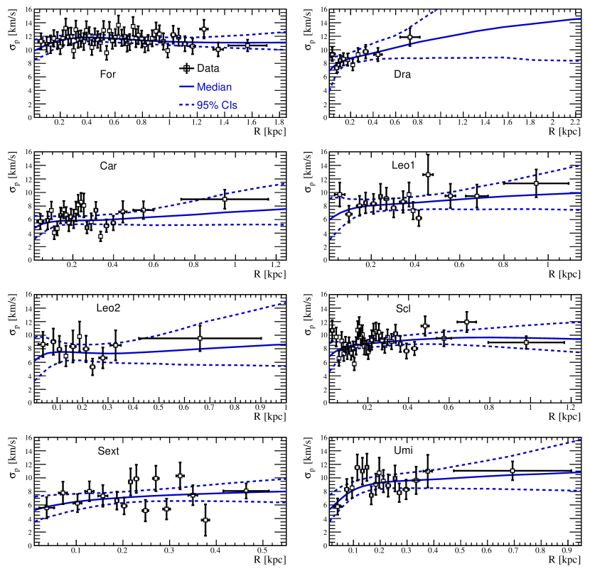
Figure 1: Velocity dispersion profiles $\sigma_{p}$ of the eight ‘classical’ dSphs: data (symbols) and reconstructed median and 95% CIs (blue lines). These profiles are shown for illustration; our results are based on an unbinned analysis.

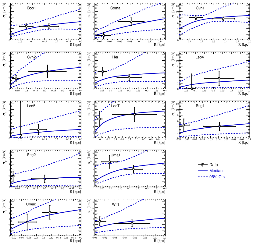
Figure 2: Velocity dispersion profiles $\sigma_{p}$ of the thirteen ‘ultrafaint’ dSphs: data (symbols) and reconstructed median and 95% CIs (blue lines). These profiles are shown for illustration; our results are based on an unbinned analysis.

4 Analysis setup

4.1 MCMC analysis

For each dSph, we perform the Jeans analysis to find the DM density profile parameters that best fit the stellar kinematics, and determine their uncertainties. The likelihood functions of the analysis (Section 2.2) have seven free parameters (see below). To efficiently explore this large parameter space, we use an MCMC technique, based on Bayesian parameter inference, which allows us to sample the PDF of a set of free parameters using Markov chains. To this purpose, we use the Grenoble Analysis Toolkit (GreAT) (Putze, 2011; Putze & Derome, 2014), which relies on the Metropolis-Hastings algorithm (Metropolis et al., 1953; Hastings, 1970). The posterior distributions are obtained after several post-processing steps (burn-in length removal, correlation length estimation, and thinning of the chains), allowing a selection of independent samples, insensitive to the initial conditions. From these PDFs, credibility intervals (CIs) for any quantity of interest can be easily computed.

For each step of the chains, we randomly select a light profile parametrisation from the accepted configurations of the MCMC analysis done previously for the surface brightness data (see Section 3), and use it for computing the velocity dispersion $\sigma_{\text{p}}$ (equation 3). This effectively propagates the light profile uncertainties to the posterior distributions of the DM and anisotropy parameters.

4.2 Free parameters and priors

The free parameters of the analysis are the three parameters of the Einasto DM density profile, and the four parameters of the Baes & van Hese (2007) velocity anisotropy profile, for which we adopt uniform priors. We follow Bonnivard et al. (2015) who after a thorough study of mock data identified an optimal prior combination that mitigates several biases introduced by the Jeans analysis. Table 1 summarises the ranges used on each parameter’s prior.

Table 1: Range of uniform priors used for the DM density and velocity anisotropy profile parameters. Note that all models must satisfy the Global Density-Slope Anisotropy Inequality (equation 17), which reduces the effective range of the anisotropy parameters. See text for details.

Quantity	Profile	Parameter	Prior range
DM density ​​​​​​	‘Einasto’ ​​​​​​​​​	$\log_{10}(\rho_{-2}/\text{M}_{\odot}~{}\text{kpc}^{-3})$​​​​​​	$[5,13]$ ​​​​​​
	equation (5) ​​​​​​​​​	$\log_{10}(\text{r}_{-2}/\text{kpc})$​​​​​​	$[\log_{10}(r_{\rm s}^{*}),1]$ ​​​​​​
		$\alpha$ ​​​​​​	$[0.12,1]$​​​​​​
Anisotropy ​​​​​​	‘Baes & van Hese’ ​​​​​​​​​	$\beta_{0}$ ​​​​​​	$[$-$9,1]$ ​​​​​​
	equation (6) ​​​​​​​​​	$\beta_{\infty}$ ​​​​​​	$[$-$9,1]$ ​​​​​​
		$\log_{10}(r_{a})$ ​​​​​​	$[$-$3,1]$ ​​​​​​
		$\eta$ ​​​​​​	$[0.1,4]$ ​​​​​​

DM density profile. Bonnivard et al. (2015) suggested two cuts on the DM density profile priors in order to tighten the constraints on the astrophysical factors without introducing bias. First, the scale radius $r_{-2}$ is forced to be larger than the scale radius of the stellar component, $r_{\rm s}^{*}$. This drastically reduces the upper CIs on the astrophysical factors for ‘ultrafaint’ dSphs. A second cut on the logarithmic slope $\alpha$, $\alpha\geq 0.12$, is also advocated in this previous work. We have chosen to use both cuts in our analysis, so as to obtain the most stringent and robust estimates of the astrophysical factors.

Velocity anisotropy profile. The priors we use for the 4 parameters of the Baes & van Hese (2007) anisotropy profiles are also those of Bonnivard et al. (2015). The generality of this parametrisation avoids the bias from the use of more specific anisotropy profiles, especially for large data samples. We also implement the Global Density-Slope Anisotropy Inequality (Ciotti & Morganti, 2010), which ensures that solutions to the Jeans equation given by our MCMC analysis correspond to physical models with positive phase-space distribution function:

$$\beta_{\text{ani}}(r)\leq-\frac{1}{2}\frac{\text{d}\log\nu(r)}{\text{d}\log(r)}.$$ (17)

This reduces the range of allowed velocity anisotropy parameters depending on the stellar number density $\nu(r)$.

4.3 Size of the DM halo

The extension of the DM halo is needed when computing the $J$- (or $D$-) factor (equation 13). The latter reaches a maximum when the integration angle $\alpha_{\rm int}$ corresponds to the angular size of the halo and saturates beyond (see figure 4, where the $J$-factor obtained for Fornax is plotted as a function of the integration angle $\alpha_{\rm int}$; the median value is seen to saturate above $\sim 1^{\circ}$).

There is no clear criterion to define the size of DM halos hence we adopt two different approaches for each dSph galaxy and for each set of DM parameters accepted by the MCMC. The first method considers the tidal radius $r_{\text{t}}$ to be a good estimator of the halo size (as shown by N-body or hydrodynamical simulations — see e.g. Springel et al. 2008; Mollitor, Nezri & Teyssier 2015); this is computed as:

$$r_{\text{t}}=\left[\frac{M_{\rm halo}(r_{\text{t}})}{[2-\text{d}\ln M_{\text{MW}}/\text{d}\ln r(d)]\times M_{\text{MW}}(d)}\right]^{(1/3)}\times d\;,$$ (18)

where $M_{\text{MW}}(d)$ is the mass of the MW enclosed within the galactocentric distance $d$ of the dSph and $M_{\rm halo}$ is the mass of the dSph galaxy. A second method to estimate the size of a DM halo consists in determining the radius $r_{\rm eq}$ where the halo density is equal to the density of the MW halo, namely,

$$\rho_{\rm DM}^{\rm halo}(r_{\rm eq})=\rho_{\rm DM}^{\rm MW}(d-r_{\rm eq}).$$ (19)

We have used both a Navarro-Frenk-White (Navarro, Frenk & White, 1997; Battaglia et al., 2005) and an Einasto profile (Navarro et al., 2004; Springel et al., 2008) for the MW density, with no impact on the results. We also find the above two estimates of the dSph galaxy size to be comparable, leading to very similar astrophysical factors (see Appendix B). Note that other assumptions can also be made to estimate the dSph halo size. For instance, in order to be conservative, Geringer-Sameth, Koushiappas & Walker (2015) used the outermost observed star as truncation radius for computing the astrophysical factors. However, this can underestimate the $J$- and $D$-factors, and may moreover underestimate the credibility intervals (see Appendix B).

4.4 Membership probabilities and impact of contamination

$J$- and $D$-factor reconstruction through Jeans analysis has been previously studied and optimised for contamination-free mock data (Charbonnier et al., 2011; Bonnivard et al., 2015). However, actual observations yield kinematic samples that may be contaminated by field stars belonging to the Milky Way or to a Galactic stream. The conventional approach to handle these interlopers relies on the arbitrary definition of some threshold separating members from outliers (sigma-clipping method, see e.g. Yahil & Vidal 1977). Expectation maximisation (EM) algorithms (Walker et al., 2009) differ from sigma-clipping methods as they provide membership probabilities $P_{i}$ for each star of the sample, which can be used as weights in subsequent analyses, e.g., equation (11). The EM algorithm was shown to provide accurate and reliable membership probabilities in most cases, although some failures may occur for samples presenting the heaviest contamination and the most overlapping velocity distributions (Walker et al., 2009).

In order to investigate whether residual contamination affects the $J$-factor values, we either use the star membership probability as weights in the likelihood function equation (11), or only retain stars which almost certainly belong to the dSph ($P_{i}>0.95$). Figure 3 compares these two approaches for dSphs with $P_{i}$ values available from the literature (eight ‘classical’ and Segue I). The same $J$-factors ($D$-factors) are reconstructed in both cases, except for Fornax and Segue I. For these two objects, the discrepancy hints at the presence of contamination in their samples that is not captured by the $P_{i}$ indicator.

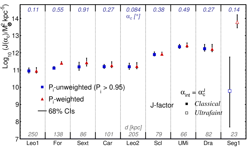
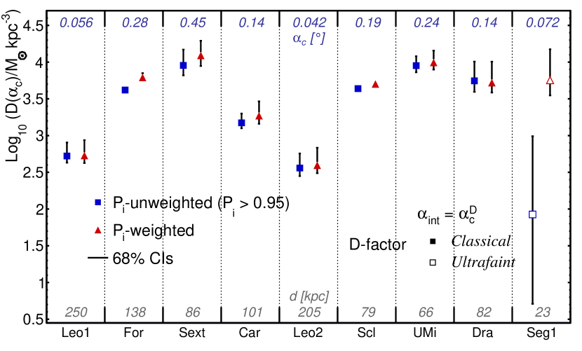
Figure 3: $J$- and $D$-factors at the critical integration angle (top and bottom panel respectively) for dSph galaxies whose $P_{i}$ values are available. Shown are values calculated using equation (11), i.e. with membership probabilities as weights in the Jeans analysis (red triangles), or using all stars passing the cut $P_{i}>0.95$ (blue squares).

The case of Segue I will be thoroughly discussed in Bonnivard, Maurin & Walker (in prep.), and we refer the reader to Appendix C for the ‘classical’ dSphs. Investigation of the stellar contamination issue is done by comparing reconstructed $J$-factors to their true values, for a set of mock data presenting different levels of Milky Way or stream contamination. Doing so, we find that:

• $J$-factors can be robustly reconstructed when large enough samples of stars are available (‘classical’ dSphs), whereas small samples (‘ultrafaint’ dSphs) are more sensitive to contamination, with their $J$- and $D$-factors more likely to overshoot the true value;

• discrepant $J$- or $D$-factors from the $P_{i}$-weighted and $P_{i}^{>0.95}$-cut analyses hint at high levels of contamination. The $P_{i}^{>0.95}$-cut analysis is found to give generally more conservative results (large CIs, but encompassing the true value) while the $P_{i}$-weighted analysis tends to overshoot (small CIs, true value outside CIs).

Therefore, in the remainder of the paper our results are based only on stars with $P_{i}>0.95$, whenever this information is available. A direct consequence of this is that Segue I (among the most favoured targets) may become one of the least reliable targets to set constraints on DM (Bonnivard, Maurin & Walker in prep.). Unsurprisingly this confirms that the ‘classical’ dSphs are the most robust targets as they are little affected by contamination.

5 Results

Using the MCMC analysis described in the previous Section, we fit the velocity data of the 8 ‘classical’ and of 13 ‘ultrafaint’ dSph galaxies with the 7 parameters (3 parameters for the Einasto DM profile and 4 for the Baes & Van Hese velocity anisotropy) required in our Jeans analysis. For each point in the chains, any relevant quantity may be computed and its median value and credibility intervals estimated from the resulting distribution.

This is true of the reconstructed velocity dispersion profile of each dSph, the median and 95% CIs of which are plotted in solid and dashed blue lines in figures 1 and 2. The reconstructed profiles and CIs appear to always provide a good representation of the data, with much wider CIs for ‘ultrafaint’ dSphs (up to a factor $\sim 5$ at large radii, compared to a factor $\sim 2$ for ‘classical’ dSphs) because of the sparsity of their stellar data.

The three Einasto profile parameters are used to compute the DM annihilation $J$-factors and decaying DM $D$-factors using equation (13). Figure 4 displays the median value and 95% CIs of the $J$- and $D$-factors, for the ‘classical’ dSph Fornax, as a function of $\alpha_{\rm int}$. Once the integration angle encompasses the whole halo, the astrophysical factors saturate. This figure shows the optimal integration angle $\alpha_{c}$ for which the CIs for the $J$- and $D$-factors are the smallest, i.e., where these astrophysical factors may be robustly determined despite our inability to constrain the inner slope of their DM profile. For Fornax, $\alpha_{c}^{D}\sim 0.28^{\circ}$ as may be seen from the figure. ASCII files of the median values, 68% and 95% CIs of $J(\alpha_{\rm int})$ and $D(\alpha_{\rm int})$ for all the dSphs discussed in this paper may be retrieved from the Supporting Information submitted with this paper.

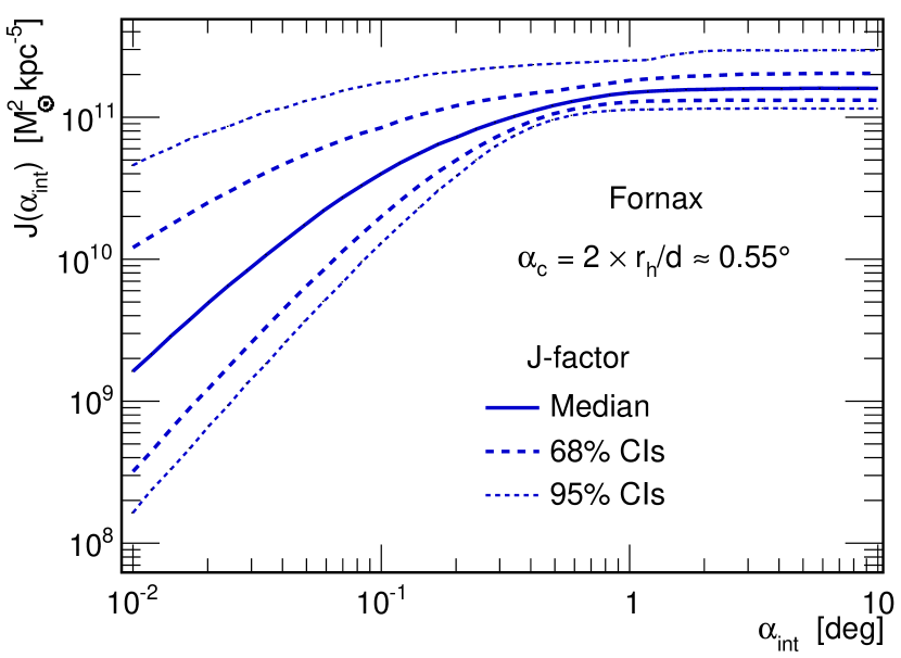
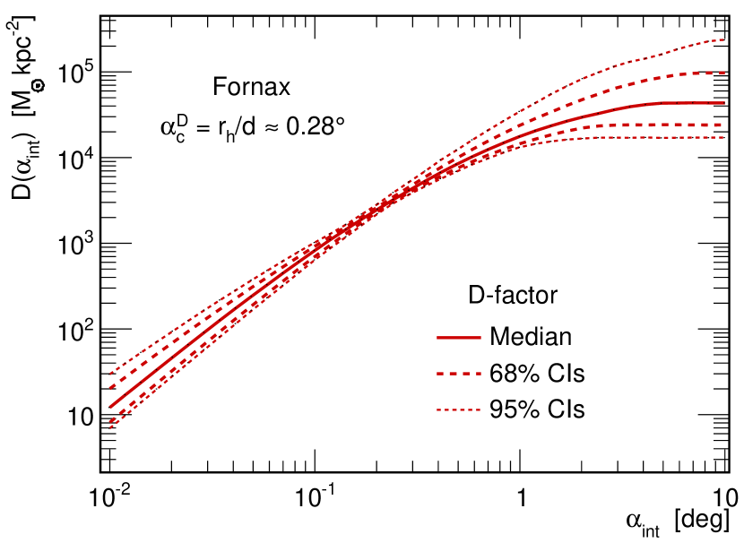
Figure 4: $J$- and $D$-factor (top and bottom panel respectively) as a function of the integration angle $\alpha_{\text{int}}$ for the ‘classical’ dSph Fornax.

5.1 J and D-factors of dSphs vs Galactic background

All the dSph satellite galaxies of the MW are embedded in its DM halo. Hence in both the annihilating and decaying DM scenario, our Galaxy’s DM halo will provide a background signal of the same nature as that of the targeted dSph galaxy. This consideration is quite independent of any diffuse $\gamma$-ray emission of astrophysical origin which we do not discuss here. For simplicity, we also ignore the extragalactic signal originating from DM annihilations or decays on cosmological scales (and integrated over all redshifts).

The MW halo’s astrophysical $J$- and $D$-factors are computed with the Clumpy code, assuming the following characteristics:

• We use an Einasto profile to model the smooth DM distribution, scaled to the local DM density ($\rho_{\odot}=0.3$ GeV cm^-3);

• We include the contribution of a population of DM clumps, having a cored spatial distribution and a mass distribution $dN/dM\propto M^{-1.9}$ (Springel et al., 2008) (amounting to $\sim 10\%$ of the MW’s total mass);

• We assume that the mass-concentration relation has a log-normal distribution (Sánchez-Conde & Prada, 2014).

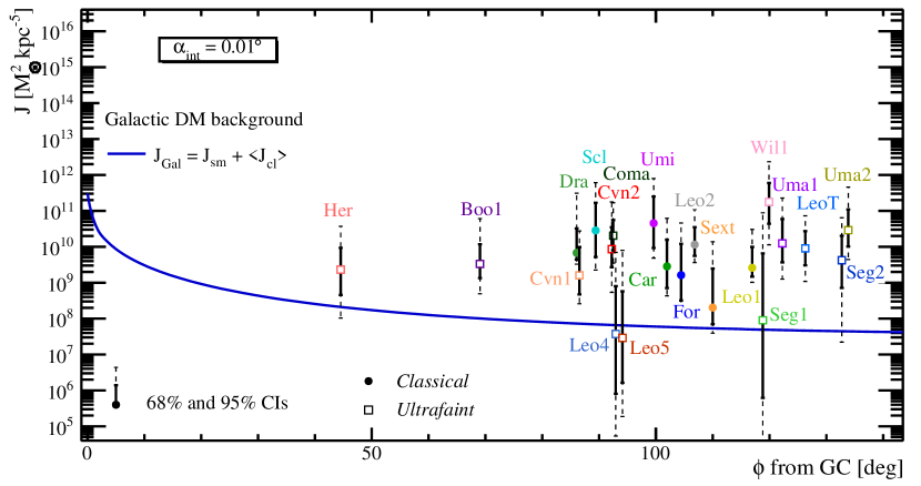
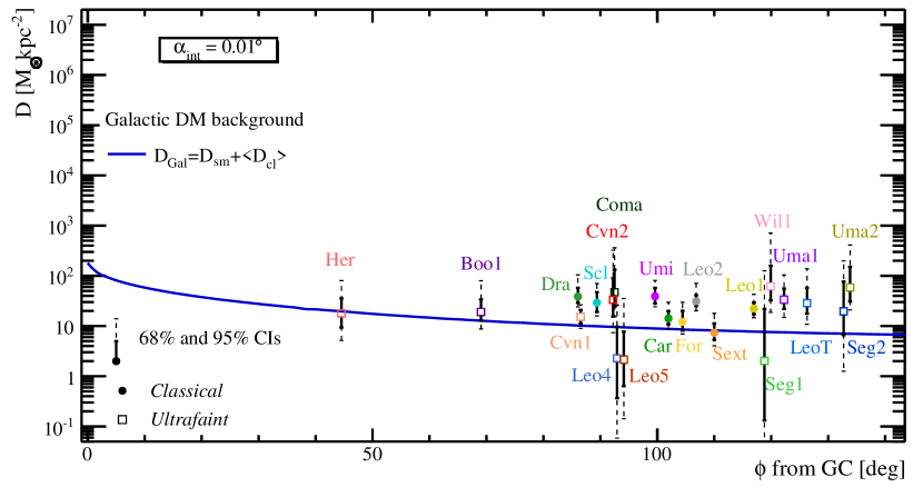
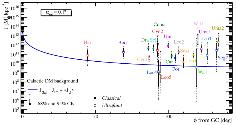
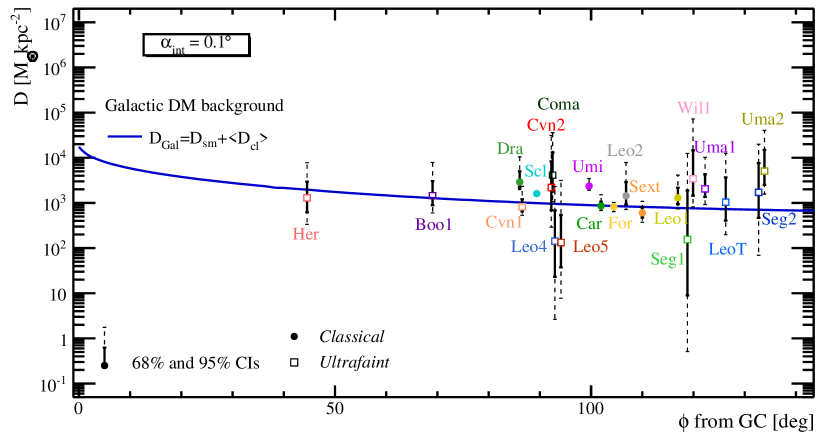
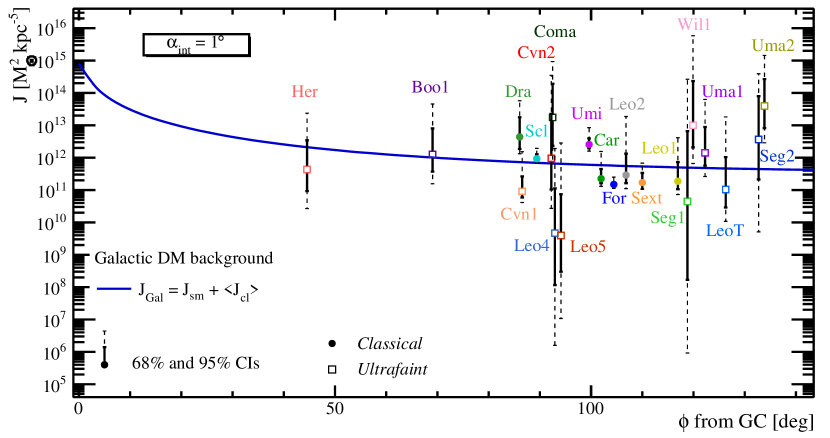
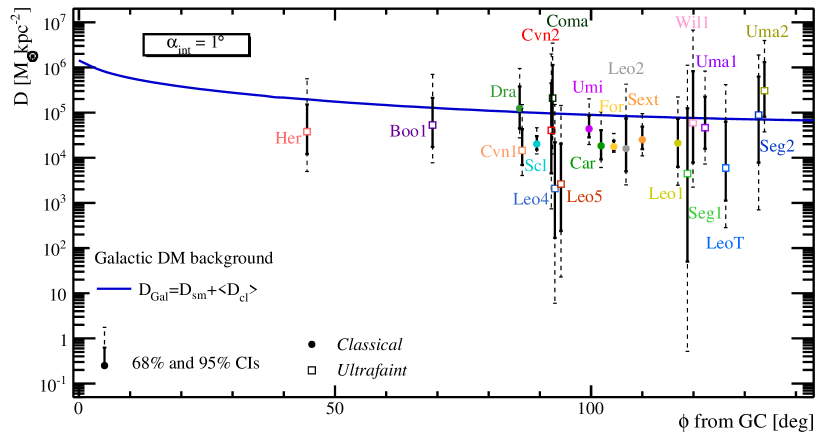
Figure 5: Annihilation (left) and decay (right) factors of the 21 dSphs studied (symbols) versus the Galactic DM halo background (blue line), as function of the angular distance from the Galactic centre. Top to bottom panels correspond to three integration angles: $0.01^{\circ}$, $0.1^{\circ}$, and $1^{\circ}$. See Section 5.1 for details.

Figure 5 displays the $J$- (left) and $D$-factors (right) of the 21 dSph galaxies (symbols) studied in this paper as a function of their angular distance from the Galactic centre. The solid blue line corresponds to our estimate of the contribution from the MW DM halo. This has been repeated for three integration angles, $\alpha_{\rm int}=0.01^{\circ},0.1^{\circ},1^{\circ}$. This figure clearly illustrates the loss of contrast between the dSph target and the MW background as the integration angle is increased. Indeed, the background (exotic or not) is $\propto\alpha_{\rm int}^{2}$; this is not so for the dSphs where the astrophysical factor is very centrally peaked, especially for $J$. For the $J$-factor, most of the dSphs appear an order of magnitude or more above the background for $\alpha_{\rm int}=0.01^{\circ}$, while this is true only of a couple of them for $\alpha_{\rm int}=1^{\circ}$. For decay (right column), even for small integration angles, the contrast is always smaller than that of annihilation. Therefore, for large integration angles which may be dictated by instrumental resolution, it would be a better strategy to look directly for the MW’s DM halo signature, rather than at a specific dSph galaxy.

5.2 J-factor: ranking of the dSphs and comparison to other works

Putting aside the notion of contrast mentioned above, the astrophysical factors are the relevant proxies to determine whether or not a given dSph is potentially interesting for indirect detection. Table 2 summarises our findings and we compare these results in figure 6 to other studies in the literature.

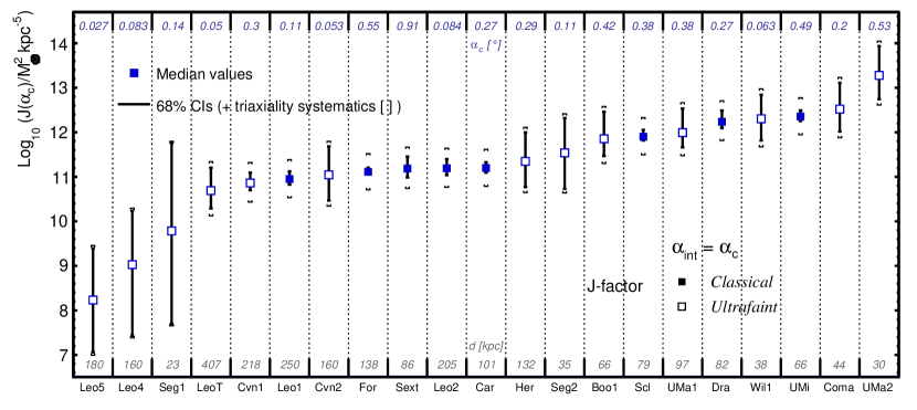
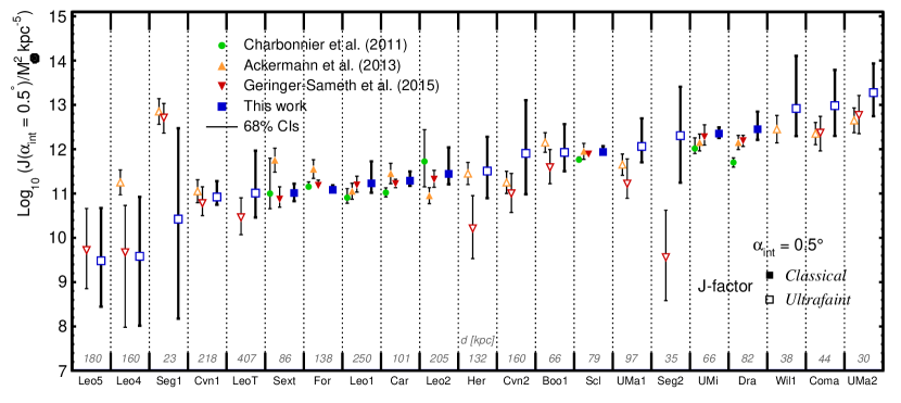
Figure 6: Top: $J$-factors and 68% CIs for $\alpha_{\text{int}}=\alpha_{c}^{J}$: the ’[]’ symbols combine in quadrature the 68% statistical uncertainties and possible systematics ($\pm 0.4$) from triaxiality of the dSph galaxies (Bonnivard et al., 2015). Bottom: comparison of the J-factors to other works, with $\alpha_{\rm int}=0.5^{\circ}$. See also Section 5.4 for a critical discussion of the targets most favoured by our analysis.

Ranking at $\alpha_{\rm int}=\alpha_{c}\approx 2r_{h}/d$.

The top panel in figure 6 shows the $J$-factors ordered according to their median from the faintest (Leo5) to the brightest (UMa2), when integrating the signal up to the optimal angle $\alpha_{\rm int}=\alpha_{c}$, where the $J$-factors have the smallest error bars. To account for possible systematics from triaxiality of the DM halo (which depends on the l.o.s. orientation of each dSph, see Bonnivard et al. 2015), the error bars (’[]’ symbols) combine a 0.4 dex uncertainty in quadrature with the 68% CIs. Our updated analysis (compared to the results presented in Charbonnier et al., 2011) still prefers UMi among all the ‘classical’ dSph while Coma and Ursa Major 2 are the most promising ‘ultrafaint’ dSphs (Segue I falls among the least interesting targets). For each dSph galaxy, the optimal angle $\alpha^{J}_{c}$ is quoted above the data point, while the distance to the dSph is quoted below. Unsurprisingly, the most promising galaxies are also among the closest. The estimated uncertainties on this plot provide a clear signature of our data-driven approach: the ‘ultrafaint’ dSphs have significantly larger error bars than their ‘classical’ counterparts.

Ranking at $\alpha_{\rm int}=0.5^{\circ}$ and comparison to other works.

The bottom panel in figure 6 compares our results to other existing studies for a fixed integration angle $\alpha_{\rm int}=0.5^{\circ}$, typical of the Fermi-LAT angular resolution in the GeV range. First, comparing the top and bottom panels shows no drastic ordering changes among the dSph galaxies but for a few inversions. Second, the overall trend appears to be preserved between the different studies, with the same objects having the highest $J$ values. Nonetheless, a closer inspection shows significant differences both in the values of the $J$-factors and the size of the error bars. The differences observed between our analysis and others is understood as follows:

• In Charbonnier et al. (2011), we conducted the same exercise on the 8 ‘classical’ dSph galaxies (green circles), but with a more constrained Jeans analysis (using a constant anisotropy profile and a Plummer light profile). UMi was found to be the most promising target among the ‘classical’ dSph, while Leo 2 had the highest median $J(\alpha_{c})$ but with much larger uncertainties. For all the objects but Leo 2 (which is very uncertain anyway), the Charbonnier et al. (2011) values are slightly lower than their updated version. Changing the anisotropy and light profiles to more flexible parametrisations in the current analysis is the main reason for the differences between this and our previous study. Overall, we find larger $J$-factors whenever the light data require an outer slope steeper than that given by the Plummer profile used in Charbonnier et al. (2011). Note that this effect was already observed on mock data in Bonnivard et al. (2015). The most striking example is the case of Draco.

• The Fermi collaboration (Fermi-LAT Collaboration, 2014, 2015) reported the $\gamma$-ray observations of 25 dSph galaxies and conducted a stacking analysis of 15 of them to set constraints on the DM annihilation cross section. These authors provide $J$-factors of 18 dSph galaxies overlapping with our sample (orange triangles), obtained using a two-level Bayesian hierarchical modelling that constraints the entire population of MW dSphs simultaneously (Martinez, 2013). Their values do not show any particular trend when compared to ours, with most CIs overlapping. The most striking difference concerns the size of their error bars, which remain roughly the same regardless of the nature of the object (‘classical’ or ‘ultrafaint’). This is very likely related to their two-level hierarchical analysis, where the entire population of MW dSph galaxies is to some extent assumed to share the same properties. The constraints coming from the ‘classical’ dSphs are therefore redistributed to the ‘ultrafaint’ dSphs. Note also that a NFW profile for the DM density was assumed, but the analysis found to be fairly insensitive to this choice.

• In Geringer-Sameth, Koushiappas & Walker (2015), the authors provide $J$- and $D$-factors of 20 dSph galaxies obtained using a data-driven Jeans analysis quite similar to ours. In particular, they use the same unbinned likelihood as in equation (10), but with a Zhao DM density profile, a constant anisotropy and a Plummer light profile. However, they select the radius of the outermost observed star as truncation radius for computing the astrophysical factors, which results in lower values (red triangles) than ours (blue squares). Segue II (Seg2), Hercules (Her), and Ursa Major I (UMa1) are particularly affected by this choice, with $R_{\text{max}}/r_{\text{h}}$ values between $\sim 2$ and $\sim 4$, while we obtain $R_{\text{max}}/r_{\text{h}}$ values $\gtrsim 10$ with our estimations of the halo size (see Section 4.3). Note that the underestimation of the halo size can also lead to an underestimation of the CIs (Appendix B). This partially explains the larger error bars we find, which are also a consequence of the more flexible anisotropy and light profiles parametrisations we use (Bonnivard et al., 2015).

In summary, figure 6 (bottom) highlights the fact that the values found for $J$-factors and their CIs can depend strongly on the underlying assumptions. We believe our present work to better reflect the various sources of uncertainties that affect $J$-factor estimations, following the thorough validation of the method initiated in Bonnivard et al. (2015) and concluded in Appendices A and B. Our data-driven analysis naturally implies larger error bars for dSphs with fewer stars, and vice-versa. Also, thanks to a more flexible parametrisation of light profile, we find higher $J$-factors for some targets, which may lower further the upper limits for the DM annihilation cross section (Fermi-LAT Collaboration, 2014; Geringer-Sameth, Koushiappas & Walker, 2014; Fermi-LAT Collaboration, 2015).

Table 2: Summary of results for the 21 dSph galaxies presented in this paper. The dSphs are ordered by distance and the columns correspond to (from left to right): name, distance, optimal angle for annihilation ($\alpha_{c}^{J}\approx 2\alpha_{c}^{D}\approx 2r_{h}/d$), median $J$-factors and 68% (95%) CIs for $\alpha_{\rm int}=0.01,\,0.5,\,\alpha_{c}^{J}$, median $D$-factors and 68% (95%) CIs for $\alpha_{\rm int}=0.01,\,0.5,\,\alpha_{c}^{D}$. Note that a systematic uncertainty of $\pm 0.4$ (resp. $\pm 0.3$) must be allowed in order to the reflect the possible triviality of the dSph galaxies (Bonnivard et al., 2015).

dSph	d	$\alpha_{c}^{J}$	$\log_{10}[J(0.01^{\circ})]$	$\log_{10}[J(0.5^{\circ})]$	$\log_{10}[J(\alpha_{c}^{J})]$ ​​		​​$\log_{10}[D(0.01^{\circ})]$​​	$\log_{10}[D(0.1^{\circ})]$	​​$\log_{10}[D(\alpha_{c}^{D})]$​​
	​​​[kpc]​​​	​​​[$\deg$]​​​	$[J/M_{\odot}^{2}\,$kpc${}^{-5}]$				$[D/M_{\odot}\,$kpc${}^{-2}]$
Segue I	23	0.14	$~{}8.0_{-2.2(-3.5)}^{+1.9(+3.0)}$	$10.4_{-2.2(-4.5)}^{+2.1(+3.5)}$	$~{}9.8_{-2.1(-3.8)}^{+2.0(+3.2)}$		$0.3_{-1.2(-2.1)}^{+1.0(+1.8)}$	$2.2_{-1.2(-2.5)}^{+1.1(+1.9)}$	$1.9_{-1.2(-2.3)}^{+1.1(+1.9)}$
Ursa Major II​​​​​​	30	0.53	$10.5_{-0.5(-0.8)}^{+0.6(+1.2)}$	$13.3_{-0.5(-0.9)}^{+0.7(+1.3)}$	$13.4_{-0.6(-1.0)}^{+0.7(+1.4)}$		$1.8_{-0.3(-0.4)}^{+0.4(+0.8)}$	$3.7_{-0.3(-0.5)}^{+0.5(+0.9)}$	$4.6_{-0.4(-0.6)}^{+0.5(+1.0)}$
Segue II	35	0.11	$~{}9.6_{-0.8(-2.3)}^{+0.7(+1.2)}$	$12.3_{-1.1(-2.7)}^{+1.1(+1.7)}$	$11.5_{-0.8(-2.3)}^{+0.8(+1.3)}$		$1.3_{-0.5(-1.2)}^{+0.6(+1.0)}$	$3.2_{-0.6(-1.4)}^{+0.6(+1.1)}$	$2.8_{-0.5(-1.3)}^{+0.6(+1.0)}$
Willman I	38	0.06	$11.2_{-0.6(-1.2)}^{+0.5(+1.1)}$	$12.9_{-0.6(-1.1)}^{+1.2(+2.3)}$	$12.3_{-0.5(-1.0)}^{+0.5(+1.2)}$		$1.8_{-0.3(-0.5)}^{+0.4(+1.1)}$	$3.5_{-0.4(-0.6)}^{+0.6(+1.3)}$	$2.8_{-0.3(-0.5)}^{+0.5(+1.2)}$
Coma	44	0.20	$10.3_{-0.4(-0.8)}^{+0.4(+0.9)}$	$13.0_{-0.7(-1.1)}^{+0.8(+1.4)}$	$12.5_{-0.5(-0.8)}^{+0.6(+1.1)}$		$1.7_{-0.3(-0.5)}^{+0.4(+0.9)}$	$3.6_{-0.4(-0.6)}^{+0.5(+0.9)}$	$3.6_{-0.4(-0.6)}^{+0.5(+0.9)}$
Ursa Minor​​​​​​	66	0.49	$10.7_{-0.7(-1.0)}^{+0.7(+1.2)}$	$12.4_{-0.1(-0.2)}^{+0.1(+0.4)}$	$12.4_{-0.1(-0.2)}^{+0.1(+0.4)}$		$1.6_{-0.1(-0.2)}^{+0.2(+0.3)}$	$3.3_{-0.0(-0.1)}^{+0.1(+0.2)}$	$4.0_{-0.1(-0.2)}^{+0.1(+0.3)}$
Boötes I	66	0.42	$~{}9.5_{-0.4(-0.8)}^{+0.5(+1.3)}$	$11.9_{-0.4(-0.8)}^{+0.6(+1.2)}$	$11.9_{-0.4(-0.7)}^{+0.6(+1.1)}$		$1.3_{-0.2(-0.3)}^{+0.3(+0.6)}$	$3.2_{-0.2(-0.4)}^{+0.3(+0.7)}$	$3.7_{-0.3(-0.5)}^{+0.4(+0.8)}$
Sculptor	79	0.38	$10.4_{-0.7(-1.1)}^{+0.8(+1.3)}$	$11.9_{-0.1(-0.1)}^{+0.1(+0.3)}$	$11.9_{-0.1(-0.1)}^{+0.1(+0.4)}$		$1.5_{-0.2(-0.3)}^{+0.2(+0.4)}$	$3.2_{-0.0(-0.1)}^{+0.0(+0.1)}$	$3.6_{-0.0(-0.1)}^{+0.0(+0.1)}$
Draco	82	0.28	$~{}9.8_{-0.2(-0.3)}^{+0.7(+1.7)}$	$12.5_{-0.2(-0.4)}^{+0.4(+0.7)}$	$12.2_{-0.1(-0.3)}^{+0.3(+0.6)}$		$1.6_{-0.1(-0.2)}^{+0.2(+0.4)}$	$3.5_{-0.1(-0.2)}^{+0.2(+0.5)}$	$3.8_{-0.2(-0.3)}^{+0.3(+0.6)}$
Sextans	86	0.91	$~{}8.3_{-0.5(-0.7)}^{+1.1(+1.8)}$	$11.0_{-0.2(-0.4)}^{+0.2(+0.4)}$	$11.2_{-0.2(-0.4)}^{+0.3(+0.6)}$		$0.9_{-0.1(-0.3)}^{+0.2(+0.4)}$	$2.8_{-0.1(-0.2)}^{+0.1(+0.3)}$	$4.0_{-0.1(-0.3)}^{+0.2(+0.4)}$
Ursa Major I​​​​​​	97	0.38	$10.1_{-0.5(-1.0)}^{+0.7(+1.3)}$	$12.1_{-0.4(-0.7)}^{+0.6(+1.3)}$	$12.0_{-0.3(-0.6)}^{+0.6(+1.2)}$		$1.5_{-0.2(-0.4)}^{+0.2(+0.5)}$	$3.3_{-0.2(-0.3)}^{+0.3(+0.7)}$	$3.8_{-0.2(-0.4)}^{+0.4(+0.8)}$
Carina	101	0.27	$~{}9.4_{-0.6(-0.8)}^{+0.7(+1.3)}$	$11.3_{-0.1(-0.2)}^{+0.2(+0.5)}$	$11.2_{-0.1(-0.2)}^{+0.1(+0.4)}$		$1.2_{-0.1(-0.2)}^{+0.1(+0.3)}$	$2.9_{-0.1(-0.1)}^{+0.1(+0.2)}$	$3.2_{-0.1(-0.1)}^{+0.1(+0.3)}$
Hercules	132	0.29	$~{}8.6_{-0.6(-1.3)}^{+0.6(+1.3)}$	$10.9_{-0.7(-1.2)}^{+0.7(+1.6)}$	$10.7_{-0.6(-1.1)}^{+0.7(+1.4)}$		$0.9_{-0.3(-0.6)}^{+0.3(+0.7)}$	$2.8_{-0.3(-0.6)}^{+0.4(+0.8)}$	$3.0_{-0.3(-0.6)}^{+0.4(+0.9)}$
Fornax	138	0.56	$~{}9.2_{-0.7(-1.0)}^{+0.9(+1.5)}$	$11.1_{-0.1(-0.1)}^{+0.1(+0.3)}$	$11.1_{-0.1(-0.1)}^{+0.1(+0.3)}$		$1.1_{-0.2(-0.2)}^{+0.2(+0.4)}$	$2.9_{-0.1(-0.1)}^{+0.0(+0.1)}$	$3.6_{-0.0(-0.0)}^{+0.0(+0.1)}$
Leo IV	160	0.08	$~{}7.6_{-1.7(-2.8)}^{+1.3(+2.3)}$	$~{}9.6_{-1.6(-3.4)}^{+1.3(+2.4)}$	$~{}9.0_{-1.6(-3.0)}^{+1.2(+2.0)}$		$0.4_{-0.8(-1.6)}^{+0.6(+1.1)}$	$2.2_{-0.8(-1.7)}^{+0.7(+1.2)}$	$1.5_{-0.8(-1.6)}^{+0.6(+1.1)}$
Canis Venatici II​​​​​​​	160	0.05	$~{}9.9_{-0.5(-1.2)}^{+0.6(+1.3)}$	$11.9_{-0.9(-1.5)}^{+1.2(+2.3)}$	$11.0_{-0.6(-1.2)}^{+0.6(+1.3)}$		$1.5_{-0.3(-0.7)}^{+0.4(+1.0)}$	$3.3_{-0.5(-0.9)}^{+0.6(+1.2)}$	$2.3_{-0.4(-0.7)}^{+0.5(+1.0)}$
Leo V	180	0.027	$~{}7.5_{-1.2(-2.2)}^{+1.3(+2.4)}$	$~{}9.5_{-1.0(-2.5)}^{+1.2(+2.7)}$	$~{}8.2_{-1.2(-2.1)}^{+1.2(+2.4)}$		$0.3_{-0.5(-1.2)}^{+0.6(+1.2)}$	$2.1_{-0.5(-1.2)}^{+0.6(+1.4)}$	$0.6_{-0.5(-1.2)}^{+0.6(+1.2)}$
Leo II	205	0.08	$10.1_{-0.3(-0.5)}^{+0.5(+1.0)}$	$11.4_{-0.2(-0.4)}^{+0.6(+1.5)}$	$11.2_{-0.2(-0.3)}^{+0.2(+0.5)}$		$1.5_{-0.1(-0.2)}^{+0.1(+0.4)}$	$3.2_{-0.2(-0.3)}^{+0.3(+0.7)}$	$2.6_{-0.1(-0.2)}^{+0.2(+0.6)}$
Canis Venatici I​​​​​​​	218	0.3	$~{}9.2_{-0.5(-0.8)}^{+0.8(+1.2)}$	$10.9_{-0.2(-0.3)}^{+0.4(+0.9)}$	$10.9_{-0.2(-0.3)}^{+0.3(+0.7)}$		$1.2_{-0.1(-0.2)}^{+0.1(+0.2)}$	$2.9_{-0.1(-0.2)}^{+0.2(+0.5)}$	$3.3_{-0.1(-0.2)}^{+0.2(+0.6)}$
Leo I	250	0.11	$~{}9.4_{-0.2(-0.4)}^{+0.6(+1.1)}$	$11.2_{-0.2(-0.4)}^{+0.5(+1.1)}$	$10.9_{-0.1(-0.2)}^{+0.2(+0.4)}$		$1.3_{-0.1(-0.2)}^{+0.1(+0.3)}$	$3.1_{-0.1(-0.2)}^{+0.2(+0.5)}$	$2.7_{-0.1(-0.2)}^{+0.2(+0.4)}$
LeoT	407	0.05	$10.0_{-0.5(-0.9)}^{+0.5(+0.9)}$	$11.0_{-0.6(-1.0)}^{+1.0(+2.1)}$	$10.7_{-0.4(-0.8)}^{+0.5(+1.1)}$		$1.5_{-0.2(-0.4)}^{+0.3(+0.7)}$	$3.0_{-0.4(-0.7)}^{+0.5(+1.1)}$	$2.1_{-0.3(-0.5)}^{+0.4(+0.8)}$

5.3 D-factor: ranking of the dSphs and comparison to other works

Dark matter decay is less often considered than annihilation, however recent observations of an unidentified X-ray line at 3.55 keV in galaxy clusters has generated increasing interest in this possibility (e.g., Bulbul et al., 2014a; Boyarsky et al., 2014b).

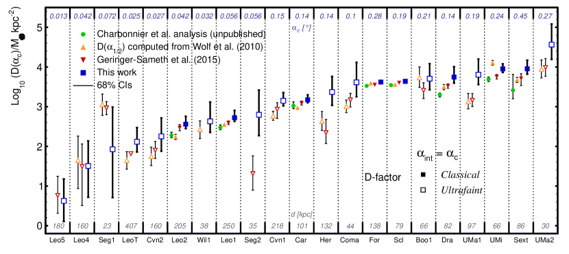
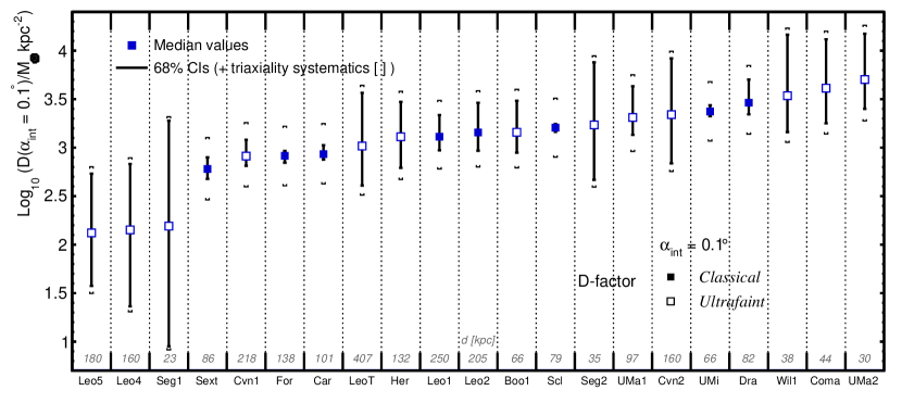
Figure 7: Top: $D$-factors and 68% CIs for $\alpha_{\text{int}}=\alpha_{c}^{D}$ and comparisons to other works Bottom: same but for $\alpha_{\text{int}}=0.1^{\circ}$: the ’[]’ symbols combine the 68% statistical uncertainties and possible systematics ($\pm 0.3$) from triaxiality of the dSph galaxies (Bonnivard et al., 2015). See also Section 5.4 for a critical discussion of the targets most favoured by our analysis.

Ranking.

The blue squares in figure 7 and the three rightmost columns of table 2 give an overview of the $D$-factors computed here. First, comparing the top panels of figures 6 and 7, we find that the ordering of the most promising targets changes significantly whether focusing on DM annihilation or decay, even though Ursa Major II remains the best candidate for $\alpha_{\rm int}=\alpha_{c}^{D}$. Furthermore, the two panels in figure 7 show that changing the integration angle for a decaying DM signal also has a strong impact on the ranking and on the error bars, more strongly than in the case of DM annihilation. In particular, for $\alpha_{\rm int}=0.1^{\circ}$ (bottom panel), most targets have very similar $D$-factors and the increased error bars make the ranking less obvious.

Comparison to other works.

The availability of independently-derived $D$-factors for dSphs in the literature remains limited, making comparison less straightforward than in the case of annihilation.

• Although not published in the Charbonnier et al. (2011) study which focused on $J$-factors only, the $D$-factors for the eight ‘classical’ dSphs were also obtained from our original analysis setup. As in the case of annihilation, these values (green dots in figure 7) are systematically lower than that obtained by the present analysis and this is connected, as for $J$, to the choice of the light profile.

• We also compare our results to those of Geringer-Sameth, Koushiappas & Walker (2015), noting again that the conservative choice made for the size of the DM halo in that study leads to a deficit in the $D$-factors compared to our values. This deficit is more apparent here than for annihilation as the outer regions of the DM halo contribute more to the $D$-factors than to the $J$-factors.

• Following the claims of X-ray line detections in galaxy clusters, Malyshev, Neronov & Eckert (2014) looked for such a signal in the dSph galaxies available in XMM-Newton data. In the absence of a signal, these authors used the mass derived from Wolf et al. (2010) and Geringer-Sameth, Koushiappas & Walker (2015) to set constraints on a sterile neutrino DM scenario. In doing so, rather than writing the $D$-factor as given by equation 13, these authors use the point-like approximation and use instead $D^{\rm point}(\alpha_{\rm int})=M_{\alpha_{\rm int}}/d^{2}$, where $d$ is the distance to the galaxy and $M_{\alpha_{\rm int}}$ is the enclosed mass. Wolf et al. (2010) provide the mass $M_{1/2}$ (and the corresponding error bars) contained within the deprojected half-light radius $r_{1/2}$, corresponding to an integration angle $\alpha_{1/2}=r_{1/2}/d$. This angle is closely related to our definition of the optimal integration for decay $\alpha^{D}_{c}=r_{h}/d$, where $r_{h}\approx 0.75\times r_{1/2}$ is the projected half-light radius. For each dSph in the Wolf et al. (2010) sample, we compute $D^{\rm point}(\alpha_{1/2})=M_{1/2}/d^{2}$ (orange triangles in figure 7). Despite the fact that $\alpha_{1/2}>\alpha^{D}_{c}$, our $D$-factors are generally higher than the ones derived from the Wolf et al. (2010) data. Computing $M_{1/2}$ from our MCMC chains provides, in general, values that are compatible with those of Wolf et al. (2010); this excludes the mass reconstruction from being the sole origin of the differences. The main remaining difference may lie in the point-like approximation, which does not account properly for the full volume of the DM halo being intercepted by the line-of-sight. While this may not be an inappropriate assumption for the strongly peaked annihilation signal, it results in a significant deficit for the $D$-factors.

5.4 Discussion

In the previous sub-sections, we presented a ranking of the Milky Way dSph satellites as potential targets for dark matter annihilation/decay surveys based on the estimated values and uncertainties of their $J$-factors or $D$-factors. However, it is important to note that while our analysis has marginalised over many of the modelling uncertainties, issues such as the dynamical status of individual dSphs and evidence pointing to cored profiles in a number of the ‘classical’ dSphs are not accounted for.

First, it is possible that some of the dSphs, especially the ‘ultrafaints’, are not currently in dynamical equilibrium. In particular, a number of authors have presented evidence that the UMa2 dSph, which occupies the top position in both the $J$- and $D$-factor rankings, is currently experiencing strong tidal disturbance by the Milky Way (Fellhauer et al., 2007; Muñoz, Geha & Willman, 2010; Smith et al., 2013). While it is not clear that this has inflated the velocity dispersion of UMa2, some caution is advisable before selecting UMa2 as a prime candidate for indirect dark matter detection surveys.

Secondly, the precise nature of some ‘ultrafaint’ galaxies is still uncertain—it is possible that some are more closely related to star clusters and do not, in fact, contain dark matter. For example, the most recent study of Wil1 describes it as ”A Probable Dwarf Galaxy with an Irregular Kinematic Distribution” and notes that foreground contamination and unusual kinematics make the determination of its dark matter content difficult (Willman et al., 2011). Target selection for dark matter surveys must take account of such uncertainty when weighting candidates for study.

The Sextans, Ursa Minor and Draco ‘classical’ dSphs feature in the top five of both the $J$- and $D$-factor rankings. The larger kinematic samples in these objects make the Jeans modelling more robust (as indicated by their smaller confidence intervals in figures 6 and 7). However, in the case of Sextans (Lora et al., 2013; Kleyna et al., 2004) and Ursa Minor (Pace et al., 2014; Kleyna et al., 2005), it has been suggested that the presence of kinematic substructures indicate that the dark matter halos of these objects are cored rather than cusped. In principle, this could be taken into account via priors on the halo slope within our Bayesian analysis, but as shown in figure 15 of Charbonnier et al. (2011), this would not actually change the conclusions for most integration angles (i.e., $\alpha_{\rm int}\gtrsim 0.1^{\circ}$).

Thus, of the seven dSphs which are within the top five of the $J$ and $D$ rankings, additional evidence for 4 of them suggests that the results of equilibrium dynamical modelling might not be sufficient to characterise their suitability as targets for indirect dark matter detection. Clearly, it is imperative that further data are obtained on potential candidates before future surveys select their target lists. New non-equilibrium modelling approaches such as that presented in Ural et al. (2015, in press) will also be important in placing the target selection on a secure footing.

6 Conclusions

Dwarf spheroidal galaxies have been widely targetted in for searches for annihilating dark matter in the Galaxy. This has enabled $\gamma$-ray telescopes to set very stringent limits on the DM annihilation cross section which are now beginning to impinge on the cosmologically preferred value for a thermal relic. Reliable estimates of the dSph $J$-factors and associated error budgets are clearly crucial in this regard. This is especially true for ‘stacking’ analyses that use data on several dSph galaxies simultaneously to improve the sensitivity. Ranking of the dSphs, according to their $J$- (and $D$-) factors, is also mandatory to optimise the strategy of pointed observations. In case of a positive detection in a given target, this will inform the strategy for subsequent observations aiming to validate the DM hypothesis.

This study — follow-up of our previous effort (Charbonnier et al., 2011) — extends and improves the reconstruction of the astrophysical factor for dSph galaxies in several ways:

• We use the optimised analysis setup proposed in Bonnivard et al. (2015): the parametrisation of the ingredients of the Jeans analysis are kept as general as possible to minimise biases. In the spirit of Charbonnier et al. (2011), we adopt very weak priors to have as data-driven an analysis as possible.

• We rely on an improved analysis of light profiles (Walker et al., in prep.) for better $J$-factor reconstruction (Bonnivard et al., 2015), and also include recent kinematic data (e.g. for Draco, see Walker, Olszewski & Mateo 2015) in the analysis.

• We test the impact of the choice of the likelihood function on the results: the performance and consistency of binned and unbinned analyses are validated on real and mock data. Furthermore, contamination from foreground stars and any associated impact on the $J$-factors are also investigated, using the membership probability of stars when available.

• In addition to the 8 ‘classical’ dSph galaxies in Charbonnier et al. (2011), re-analysed here, the results for 13 ‘ultrafaint’ dSphs are now also provided — both the $J$-factors for annihilating DM and the $D$-factors for decaying candidates.

The most important result of our study is the ranking (median and CIs) of the astrophysical factors shown in figures 6 (annihilation) and 7 (decay), and summarised in Table 2. ASCII files for the median and 68% and 95% CIs for a large range of integration angles can be retrieved from the Supporting Information submitted with this paper. Our findings can be summarised thus:

1. The unbinned Jeans analysis of stars whose membership probability is $>0.95$ gives the most stringent constraints and is appropriate to deal conservatively with possible contaminations.

2. Our $J$- and $D$-factors are in general consistent with other calculations, though several differences are observed: using a more flexible light profile (cf. the usually adopted Plummer profile) slightly increases the astrophysical factor for several dSphs; using a more flexible anisotropy profile (w.r.t. the usually assumed constant) slightly enlarges the $J$-factor CIs, providing more realistic uncertainties. This also mitigates possible biases (Bonnivard et al., 2015).

3. Uncertainties on the astrophysical factors ($J$ and $D$) from this data-driven analysis are directly related to the sample size used for the analysis (large error bars for ‘ultrafaints’, small error bars for ‘classicals’). We believe this better accommodates a possible non-universality in the properties of these objects.

4. The ranking of the targets (according to their median values) slightly depends on the integration angle. At the optimal angle $\alpha_{c}^{J}\approx 2r_{h}/d$, the ‘classical’ dSphs UMi and Draco are confirmed as the potentially-brightest and most favoured targets in terms of $J$-factors. The ‘ultrafaint’ objects UMa 2 and Coma outrank them, but suffer from larger uncertainties, and in particular their lower 95% CIs are lower than those of UMi or Draco. For decaying DM, Sextans appears as the brightest ‘classical’ dSph at $\alpha_{c}^{D}\approx r_{h}/d$, while UMa 2 remains the brightest ‘ultrafaint’ target. Not discussed here is the frequency-dependent astrophysical background that may affect this ranking. This would require an instrument-specific analysis that goes beyond the scope of this paper.

5. The astrophysical factors of Segue I might be highly uncertain due to probable stellar contamination and few kinematic data, and this object does not make it among the top ten targets (Bonnivard, Maurin & Walker, in prep.). (Re)-analyses of membership probabilities for other ‘ultrafaints’ would be helpful to probe the level of contamination in these objects.

The 9 new potential dSphs discovered in the DES survey (DES Collaboration et al., 2015; Koposov et al., 2015) and already searched for in Fermi-LAT data (Fermi-LAT Collaboration et al., 2015; Geringer-Sameth et al., 2015) call for a continued effort on this topic (see also Laevens et al. 2015; Martin et al. 2015; Kim et al. 2015 for three other recently discovered dSphs). Careful studies of their astrophysical factors will likely be difficult due to the small amount of kinematic data expected for these objects. As underlined in this study, it is all the more important to explore the limitations of kinematic analyses for such small stellar samples. This may prove crucial to understand whether the recently published limits from 6 years of Fermi-LAT observations on 15 dSphs (Geringer-Sameth, Koushiappas & Walker, 2014; Fermi-LAT Collaboration, 2015) can be significantly improved or not, and/or if better targets exist for the forthcoming Cherenkov Telescope Array (Actis et al., 2011).

Appendix A Unbinned analysis - validation on mock data

Bonnivard et al. (2015) thoroughly tested the Jeans analysis using binned velocity dispersion profiles (see equation 8), but unbinned analyses (equation 10) are also often used in the literature (e.g. Strigari et al. 2008; Martinez et al. 2009; Geringer-Sameth, Koushiappas & Walker 2015). Here, we conduct a careful comparison using a large set of mock data to determine the merits and limits of each approach, and select the optimal setup for our analysis.

Mock data set

To this purpose, we employed the same suite of mock data set used previously by Walker et al. (2011); Charbonnier et al. (2011); Bonnivard et al. (2015). It consists of 64 models covering a large variety of DM density profiles (from cored to NFW-like cuspy profiles), stellar light profiles and velocity anisotropy values (between $\beta_{\text{ani}}=-0.45$ and $\beta_{\text{ani}}=+0.3$, with constant anisotropy). We refer the reader to the papers quoted above for a more complete description of this mock data set. For each model, we draw samples of $N=30$ (small), $1000$ (medium) and $10000$ (large) stars, mimicking ‘ultrafaint’, ‘classical’ and ‘ideally observed’ dSphs. No foreground contamination is added to the data sets, and all the objects are fixed to a distance $d=100$ kpc.

Analysis setup

For each 64 mock models and sample sizes combination, we run the Jeans analysis using either the binned or unbinned likelihood functions described in Section 2.2 (see Eqs. 8 and 10 respectively). We fix the light and anisotropy parameters to their true values (i.e. the ones used to generate the mock data), in order to disentangle the effects of the likelihood functions to that originating from the physical parameters. For each model we then compute the $J$- and $D$-factors as a function of the integration angle $\alpha_{\rm int}$.

Effects of unbinned analysis

First, we find that using either the binned or the unbinned likelihood function leads to very similar results for the 64 models, regardless of the sample size. This is illustrated in figure 8, by comparing the $J$-factors obtained using either the binned (blue filled circles) or the unbinned (red empty circles) analysis to the true value (solid back line, computed using the DM parameters used to generate the mock data), for a typical ‘ultrafaint’-like mock dSph.

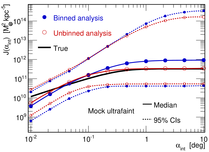
Figure 8: Median value (solid) and 95% CIs (dashed) of the $J$-factors as a function of the integration angle $\alpha_{\rm int}$, reconstructed using either a binned (blue filled circles) or an unbinned (red empty circles) Jeans analysis on a mock ‘ultrafaint’ dSph. Both analyses lead to very similar results, with the true $J$-factor (black) being encompassed within the reconstructed CIs.

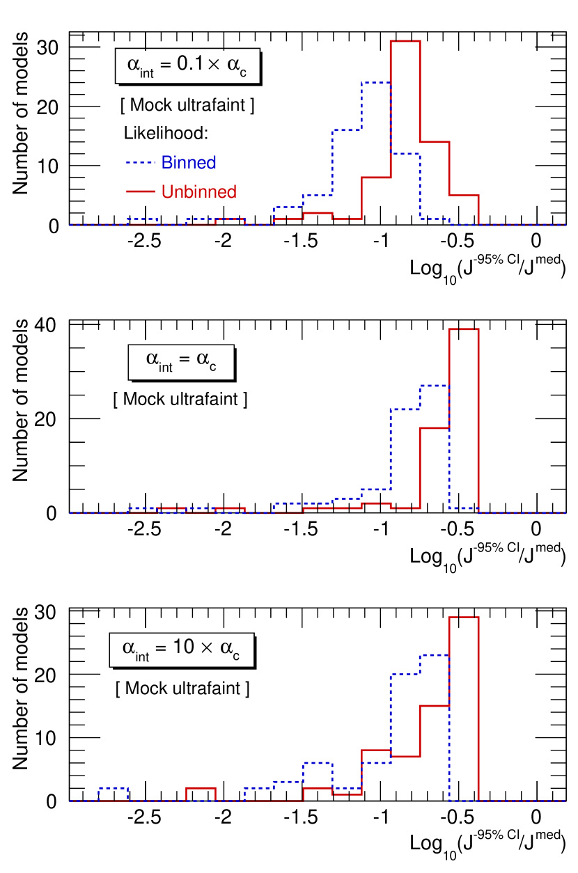
Figure 9: Distributions of $J^{-95\%\rm CI}/J^{\rm med}$, obtained for the 64 mock ‘ultrafaint’ dSphs using either the binned (dashed blue) or the unbinned (solid red) analysis. For the three integration angles considered ($\alpha_{\rm int}=0.1\times\alpha_{c}$, $\alpha_{c}$ and $10\times\alpha_{c}$, from top to bottom), the unbinned analysis allows to reduce the mean $J^{-95\%\rm CI}/J^{\rm med}$ by a factor two. The effect is much less pronounced for larger data sets.

The main difference between the two analyses lies in the CIs, as the unbinned analysis is found to be more constraining than the binned approach for ‘ultrafaint-like’ dSphs. We show in figure 9 the distributions of $J^{-95\%\rm CI}/J^{\rm med}$, i.e. the ratio of the lower 95% CI to the median $J$-factor, obtained for the 64 mock ‘ultrafaint’ dSphs using either the binned (dashed blue) or the unbinned (solid red) analysis. The integration angle is set to $0.1\times\alpha_{c}$ (top), $\alpha_{c}$ (middle) and $10\times\alpha_{c}$ (bottom). For each integration angle, the mean value of $J^{-95\%\rm CI}/J^{\rm med}$ is reduced by a factor two for the mock ‘ultrafaint’ dSphs when using the unbinned analysis. The effect is much less pronounced for the medium (‘classical’-like) and large data samples. We note a similar effect on the upper 95 % CIs (not shown). For the $D$-factors, the effect is also present for the ‘ultrafaint’-like dSphs, but less so, with a reduction of the CIs by $\sim 30\%$ when using the unbinned analysis.

Finally, we have checked that no bias is introduced when using the unbinned analysis on the 64 mock models. We therefore advocate the use of the unbinned analysis when dealing with small data samples, as it allows a significant reduction of the statistical uncertainties.

Appendix B Size of the DM halo

As pointed out in Section 4.3, the way one defines the DM halo size could influence the values of the astrophysical factors. In order to quantify this effect, we performed several tests on the mock dataset described in Appendix A.

Impact of halo size on $J$- and $D$-factors: tests on mock data

First, using two typical mock models (with either cuspy or core DM density profile), and for three different choices of halo maximum radius $R_{\text{max}}$, we compute the $J$-factor as a function of the integration angle $\alpha_{\rm int}$. Figure 10 compares the results to a reference value obtained with $R_{\text{max}}^{\rm ref}=50\times r_{s}^{*}$, chosen arbitrarily. Unsurprisingly it shows that an underestimation of the halo size leads to an underestimation of the $J$-factor, the effect being stronger for the core than for the cuspy DM profile. The $J$-factor can be underestimated by up to 70% at the critical angle $\alpha_{c}$ for a core profile and a halo size strongly underestimated (factor 25 too small). The effect is even more important for the $D$-factors (underestimation by $\sim 80\%$ at $\alpha_{c}$ for the same model mentioned before, not shown).

To evaluate the response of the CIs of the $J$-factors to the halo size, we run the Jeans analysis on the entire set of mock dSphs (see Appendix A). For each mock dSph, we fix three values of $R_{\text{max}}$, and compute the $J$-factors and their CIs from the reconstructed DM density profiles. We show in figure 11 the distributions of $J^{+95\%\rm CI}/J^{\rm med}$ for the three halo sizes, i.e. the ratio of the upper 95% CI to the median value, obtained for the 64 mock ‘ultrafaint’ dSphs at $\alpha_{\rm int}=5\times\alpha_{c}$. For this large integration angle, the credibility intervals shrink when the halo size gets smaller, so that an underestimation of the halo size will also lead to an underestimation of the credibility intervals. For the $J$-factors, this effect appears only at large integration angles ($\alpha_{\rm int}>\alpha_{c}$). For the $D$-factors, the effect is more pronounced, and appears at all integration angles (not shown).

Halo size estimation: comparison of the two methods

In this work, we have considered two methods to estimate the halo size, detailed in Section 4.3. The first method uses the tidal radius as an estimation of the physical size of the halo; in the second approach, it is evaluated as the radius where the halo DM density and the MW DM density are equal. For a given dSph galaxy, the halo size is computed for each DM model accepted by the MCMC analysis. Figure 12 shows the distributions of $R_{\text{max}}$ values obtained for Ursa Minor, using either the tidal radius estimation (red solid) or the equality of DM densities (dashed blue). Both distributions spread over more than one order of magnitude, with the mean of tidal radii distribution being systematically larger than the mean estimation from the DM density equality. This behaviour is found in all the dSphs. This trend is however not reflected on the astrophysical factors, for which both methods give very similar results as shown in the bottom panel in figure 12.

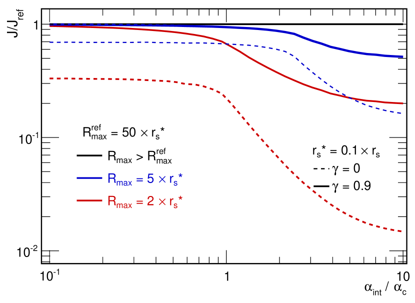
Figure 10: Ratios of $J$-factors obtained with three different halo sizes $R_{\text{max}}$ (in black, blue and red colours) to a reference $J$-factor with $R_{\text{max}}^{\rm ref}=50\times r_{s}^{*}$. The smaller is $R_{\text{max}}/R_{\text{max}}^{\rm ref}$, the more underestimated is the $J$-factor. The effect is stronger for core (dashed lines) than for cuspy DM profiles (continuous lines).

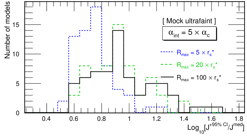
Figure 11: Distributions of $J^{+95\%\rm CI}/J^{\rm med}$ obtained for the 64 mock ‘ultrafaint’ dSphs at $\alpha_{\rm int}=5\times\alpha_{c}$. Three halo sizes are considered (short dashed blue, $R_{\text{max}}=5\times r_{s}^{*}$; long dashed green, $R_{\text{max}}=20\times r_{s}^{*}$; solid black, $R_{\text{max}}=100\times r_{s}^{*}$). At such large integration angles, smaller halo sizes reduce the credibility intervals. Underestimation of the halo size can then lead to underestimation of the CIs.

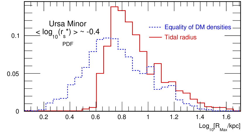
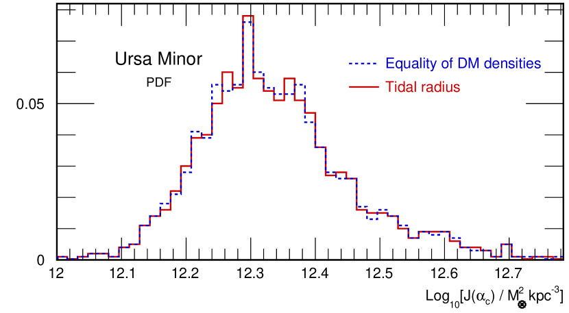
Figure 12: Top: Distribution of halo sizes obtained for Ursa Minor, using either the tidal radius (solid red) or the DM densities equality (dashed blue) estimation. Both distributions show a large spread over one order of magnitude, with the mean of the tidal radii distribution systematically larger than the mean estimation with the DM densities. Note that the mean light scale radius $\langle r_{s}^{*}\rangle$ (obtained by fitting the surface brightness data) is typically one order of magnitude lower than halo sizes derived here. Bottom: Same as upper panel but for the $J$-factors. The systematic shift noted in the halo size does not propagate to the astrophysical factors.

Appendix C Impact of contamination for ‘classical’-like dSph galaxies

Samples of stars from dSph galaxies may be contaminated by Milky Way and/or stream interlopers. Contamination in the context of Segue I will be discussed in Bonnivard, Maurin & Walker (in prep.). The less spectacular case of Fornax is presented below.

Low impact contamination in Fornax

Figure 13 shows the $J$-factors for Fornax from both the $P_{i}$-weighted (red cross) and $P_{i}$-unweighted (cut $P_{i}>0.95$, black circles) analyses. Contrarily to the other ‘classical’ dSphs, the two analyses give results which are in slight disagreement at the two-sigmas level (especially at large radii). The lower panels of figure 13 show the membership probabilities as a function of the projected radius $R$ for Fornax (middle panel) and Carina (bottom panel): 7 out of the 8 ‘classical’ dSph data display similar properties as Carina, i.e. most of the stars have $P_{i}\gtrsim 0.95$ with velocities close to the mean value $\langle v\rangle$ for the object. Fornax shows a significant fraction of stars with intermediate $P_{i}$ values (especially at large radii), whose velocity departs from the average. This is at the origin of the difference between the two reconstructed $J$-factors (top panel). Segue I shows a much stronger dependence on the type of analysis, as will be discussed in Bonnivard, Maurin & Walker (in prep.).

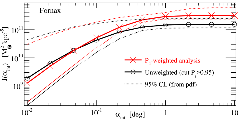
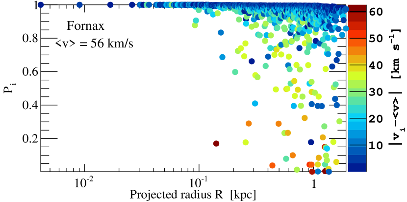
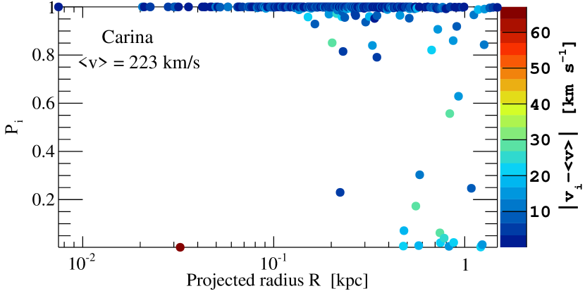
Figure 13: Top panel: $J$-factor as a function of the integration angle $\alpha_{\text{int}}$ for the ‘classical’ dSph Fornax, for an analysis with and without weighting by membership probabilities (see text). The lower panels show the membership probability $P_{i}$ of Fornax and Carina stars as a function of the projected radius $R$. The colour scale indicates the departure (red) from the mean velocity $\langle v\rangle$ of all stars (blue).

Impact of contamination checked on mock data

Jeans analyses on mock data with controlled levels of contaminant are helpful to investigate the impact and/or robustness of the reconstructed $J$-factors. Among the contaminant-free mock data described in Bonnivard et al. (2015), we selected a couple of models (with rising, flat, or decreasing velocity dispersion, from a core and cusp DM profile) mixed with MW and stream stars (details will be presented in Bonnivard, Maurin & Walker in prep.). For each model, we created 1000 data sets with different levels of contamination from the MW and from the stream (denoted $f_{\rm MW}$ and $f_{\rm stream}$ respectively, with $f_{\rm MW}+f_{\rm stream}\leq 1$). Two sample sizes were drawn to mimic ‘classical’ ($\sim 300-3000$ stars) and ‘ultrafaint’ ($\sim 30-100$ stars) dSph galaxies. After reconstructing membership probabilities with the EM algorithm (Walker et al., 2009), we selected the contaminated mock data that have at least 10% of their stars with intermediate membership probabilities (0.1 $\leq P_{i}\leq$ 0.95). The other sets of contaminated data correspond to a sample whose $P_{i}$ are reconstructed with high certainty (similar to no contamination case). We then ran the Jeans analysis, fixing the light and anisotropy profiles parameters to their true values to factor out non-essential ingredients of the analysis.

The results for the small sample sizes, in the context of Segue I’s analysis, will be presented in Bonnivard, Maurin & Walker (in prep.). Here, we present the result for the larger sample sizes in relation to Fornax, and show that $J$-factors for such samples are much less affected by contamination. Figure 14 shows a comparison of the reconstructed to the true value for both the $P_{i}$-weighted and $P_{i}$-unweighted (cut $P_{i}>0.95$) Jeans analyses on adversely contaminated mock data: the former analysis relies on the likelihood function equation (11), while the second takes care of removing all stars with $P_{i}\leq 0.95$. The maximal departure from the true value is observed close to maximum contamination (dashed line is $f_{\rm MW}+f_{\rm stream}=1$). However, even in this worst case, the overshoot is within a factor 10 for most of the models. Four models show more important overshooting (up to a factor $10^{3}$), which are caused by a few misidentified contaminant stars with both large departure from the mean velocity (up to 100 km/s) and large membership probability. These stars could be easily identified and removed from a real data sample. We checked that none of the ‘classical’ dSph we studied had such extreme outliers.

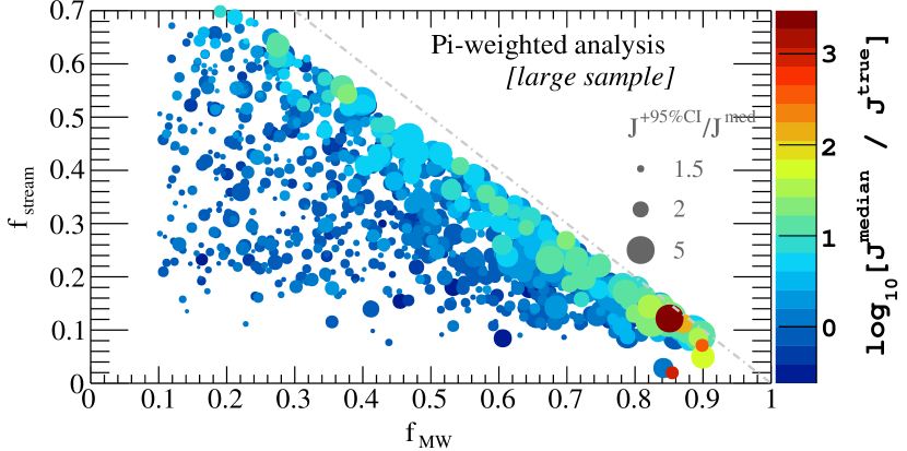
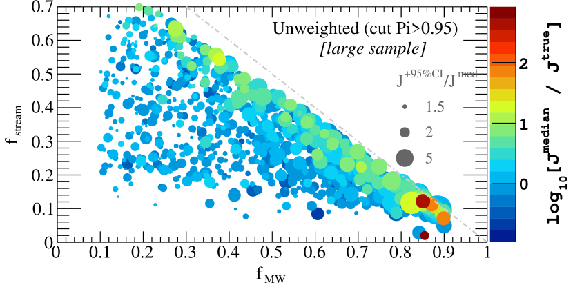
Figure 14: Analysis of reconstructed $J$-factors ($\alpha_{\rm int}=\alpha_{c}\approx 2r_{h}/d$, large sample size) of contaminated mock data. The $x$-axis (resp. $y$-axis) is the level of contamination from the Milky-Way (resp. stream) in the sample. The colour scale shows the ratio of the reconstructed to the true $J$ value. The size of the symbols correspond to the size of the CI on the reconstructed $J$-factor. See text for the discussion.

This leads to the conclusion that objects with a significant number of stars, as a result of having their membership probabilities robustly recovered (Walker et al., 2009), have a robustly reconstructed $J$-factor, even in the presence of large contamination. Regardless of the sample size, another conclusion is that whenever the fraction of stars with intermediate membership probabilities (0.1 $\leq P_{i}\leq$ 0.95) becomes significantly different from zero, the $P_{i}-R-|\Delta v|$ plot is useful to identify likely contaminated objects: in the case of ‘ultrafaint’ dSph galaxies, the impact on the $J$-factor can be very important (Bonnivard, Maurin & Walker in prep.).

References

- Abramowski et al. (2014) Abramowski A. et al., 2014, Phys. Rev. D, 90, 112012
- Actis et al. (2011) Actis M. et al., 2011, Experimental Astronomy, 32, 193
- Adén et al. (2009) Adén D., Wilkinson M. I., Read J. I., Feltzing S., Koch A., Gilmore G. F., Grebel E. K., Lundström I., 2009, ApJ, 706, L150
- Agnello & Evans (2012) Agnello A., Evans N. W., 2012, ApJ, 754, L39
- Aleksić et al. (2014) Aleksić J., Ansoldi S., Antonelli L., Antoranz P., Babic A., et al., 2014, J. Cosmology Astropart. Phys., 2, 8
- Amorisco, Agnello & Evans (2013) Amorisco N. C., Agnello A., Evans N. W., 2013, MNRAS, 429, L89
- Baes & van Hese (2007) Baes M., van Hese E., 2007, A&A, 471, 419
- Battaglia, Helmi & Breddels (2013) Battaglia G., Helmi A., Breddels M., 2013, New A Rev., 57, 52
- Battaglia et al. (2005) Battaglia G. et al., 2005, MNRAS, 364, 433
- Battaglia et al. (2008) Battaglia G., Helmi A., Tolstoy E., Irwin M., Hill V., Jablonka P., 2008, ApJ, 681, L13
- Bergström (2012) Bergström L., 2012, Annalen der Physik, 524, 479
- Bergström, Ullio & Buckley (1998) Bergström L., Ullio P., Buckley J. H., 1998, Astroparticle Physics, 9, 137
- Binney & Tremaine (2008) Binney J., Tremaine S., 2008, Galactic Dynamics: Second Edition. Princeton University Press
- Bonnivard et al. (2015) Bonnivard V., Combet C., Maurin D., Walker M. G., 2015, MNRAS, 446, 3002
- Boyarsky et al. (2014a) Boyarsky A., Franse J., Iakubovskyi D., Ruchayskiy O., 2014a, ArXiv e-prints, 1408.4388
- Boyarsky, Iakubovskyi & Ruchayskiy (2012) Boyarsky A., Iakubovskyi D., Ruchayskiy O., 2012, Physics of the Dark Universe, 1, 136
- Boyarsky et al. (2014b) Boyarsky A., Ruchayskiy O., Iakubovskyi D., Franse J., 2014b, Physical Review Letters, 113, 251301
- Breddels & Helmi (2014) Breddels M. A., Helmi A., 2014, ApJ, 791, L3
- Bulbul et al. (2014a) Bulbul E., Markevitch M., Foster A., Smith R. K., Loewenstein M., Randall S. W., 2014a, ApJ, 789, 13
- Bulbul et al. (2014b) Bulbul E., Markevitch M., Foster A. R., Smith R. K., Loewenstein M., Randall S. W., 2014b, ArXiv e-prints, 1409.4143
- Charbonnier et al. (2011) Charbonnier A. et al., 2011, MNRAS, 418, 1526
- Charbonnier, Combet & Maurin (2012) Charbonnier A., Combet C., Maurin D., 2012, Computer Physics Communications, 183, 656
- Ciotti & Morganti (2010) Ciotti L., Morganti L., 2010, MNRAS, 408, 1070
- Cirelli (2012) Cirelli M., 2012, Pramana, 79, 1021
- Cline & Frey (2014) Cline J. M., Frey A. R., 2014, Phys. Rev. D, 90, 123537
- Cole et al. (2012) Cole D. R., Dehnen W., Read J. I., Wilkinson M. I., 2012, MNRAS, 426, 601
- Combet et al. (2012) Combet C., Maurin D., Nezri E., Pointecouteau E., Hinton J. A., White R., 2012, Phys. Rev. D, 85, 063517
- DES Collaboration et al. (2015) DES Collaboration et al., 2015, ArXiv e-prints, 1503.02584
- Dotter et al. (2008) Dotter A., Chaboyer B., Jevremović D., Kostov V., Baron E., Ferguson J. W., 2008, ApJS, 178, 89
- Essig, Sehgal & Strigari (2009) Essig R., Sehgal N., Strigari L. E., 2009, Phys. Rev. D, 80, 023506
- Essig et al. (2010) Essig R., Sehgal N., Strigari L. E., Geha M., Simon J. D., 2010, Phys. Rev. D, 82, 123503
- Evans, Ferrer & Sarkar (2004) Evans N. W., Ferrer F., Sarkar S., 2004, Phys. Rev. D, 69, 123501
- Fellhauer et al. (2007) Fellhauer M. et al., 2007, MNRAS, 375, 1171
- Fermi-LAT Collaboration (2015) Fermi-LAT Collaboration, 2015, ArXiv e-prints, 1503.02641
- Fermi-LAT Collaboration et al. (2015) Fermi-LAT Collaboration et al., 2015, ArXiv e-prints, 1503.02632
- Fermi-LAT Collaboration (2014) Fermi-LAT Collaboration A., 2014, Phys. Rev. D, 89, 042001
- Feroz & Hobson (2008) Feroz F., Hobson M. P., 2008, MNRAS, 384, 449
- Feroz, Hobson & Bridges (2009) Feroz F., Hobson M. P., Bridges M., 2009, MNRAS, 398, 1601
- Feroz et al. (2013) Feroz F., Hobson M. P., Cameron E., Pettitt A. N., 2013, ArXiv e-prints, 1306.2144
- Geringer-Sameth, Koushiappas & Walker (2014) Geringer-Sameth A., Koushiappas S. M., Walker M. G., 2014, ArXiv e-prints, 1410.2242
- Geringer-Sameth, Koushiappas & Walker (2015) Geringer-Sameth A., Koushiappas S. M., Walker M. G., 2015, ApJ, 801, 74
- Geringer-Sameth et al. (2015) Geringer-Sameth A., Walker M. G., Koushiappas S. M., Koposov S. E., Belokurov V., Torrealba G., Wyn Evans N., 2015, ArXiv e-prints, 1503.02320
- Goerdt et al. (2006) Goerdt T., Moore B., Read J. I., Stadel J., Zemp M., 2006, MNRAS, 368, 1073
- Gunn et al. (1978) Gunn J. E., Lee B. W., Lerche I., Schramm D. N., Steigman G., 1978, ApJ, 223, 1015
- Hastings (1970) Hastings W. K., 1970, Biometrika, 57, 97
- Hernquist (1990) Hernquist L., 1990, ApJ, 356, 359
- Hooper (2012) Hooper D., 2012, Physics of the Dark Universe, 1, 1
- Hooper & Linden (2015) Hooper D., Linden T., 2015, ArXiv e-prints, 1503.06209
- Irwin & Hatzidimitriou (1995) Irwin M., Hatzidimitriou D., 1995, MNRAS, 277, 1354
- Jeltema & Profumo (2014) Jeltema T. E., Profumo S., 2014, ArXiv e-prints, 1408.1699
- Kim et al. (2015) Kim D., Jerjen H., Mackey D., Da Costa G. S., Milone A. P., 2015, ArXiv e-prints, 1503.08268
- Kleyna et al. (2004) Kleyna J. T., Wilkinson M. I., Evans N. W., Gilmore G., 2004, MNRAS, 354, L66
- Kleyna et al. (2005) Kleyna J. T., Wilkinson M. I., Evans N. W., Gilmore G., 2005, ApJ, 630, L141
- Kleyna et al. (2003) Kleyna J. T., Wilkinson M. I., Gilmore G., Evans N. W., 2003, ApJ, 588, L21
- Klimentowski et al. (2007) Klimentowski J., Łokas E. L., Kazantzidis S., Prada F., Mayer L., Mamon G. A., 2007, MNRAS, 378, 353
- Koposov et al. (2015) Koposov S. E., Belokurov V., Torrealba G., Wyn Evans N., 2015, ArXiv e-prints, 1503.02079
- Laevens et al. (2015) Laevens B. P. M. et al., 2015, ApJ, 802, L18
- Lake (1990) Lake G., 1990, Nature, 346, 39
- Lora et al. (2013) Lora V., Grebel E. K., Sánchez-Salcedo F. J., Just A., 2013, ApJ, 777, 65
- Madau, Shen & Governato (2014) Madau P., Shen S., Governato F., 2014, ApJ, 789, L17
- Malyshev, Neronov & Eckert (2014) Malyshev D., Neronov A., Eckert D., 2014, Phys. Rev. D, 90, 103506
- Martin et al. (2015) Martin N. F. et al., 2015, ArXiv e-prints, 1503.06216
- Martinez (2013) Martinez G. D., 2013, ArXiv e-prints, 1309.2641
- Martinez et al. (2009) Martinez G. D., Bullock J. S., Kaplinghat M., Strigari L. E., Trotta R., 2009, Journal of Cosmology and Astro-Particle Physics, 6, 14
- Maurin et al. (2012) Maurin D., Combet C., Nezri E., Pointecouteau E., 2012, A&A, 547, A16
- McConnachie (2012) McConnachie A. W., 2012, AJ, 144, 4
- Merritt et al. (2006) Merritt D., Graham A. W., Moore B., Diemand J., Terzić B., 2006, AJ, 132, 2685
- Metropolis et al. (1953) Metropolis N., Rosenbluth A. W., Rosenbluth M. N., Teller A. H., Teller E., 1953, Journal of Chemical Physics, 21, 1087
- Mollitor, Nezri & Teyssier (2015) Mollitor P., Nezri E., Teyssier R., 2015, MNRAS, 447, 1353
- Muñoz, Geha & Willman (2010) Muñoz R. R., Geha M., Willman B., 2010, AJ, 140, 138
- Navarro, Eke & Frenk (1996) Navarro J. F., Eke V. R., Frenk C. S., 1996, MNRAS, 283, L72
- Navarro, Frenk & White (1997) Navarro J. F., Frenk C. S., White S. D. M., 1997, ApJ, 490, 493
- Navarro et al. (2004) Navarro J. F. et al., 2004, MNRAS, 349, 1039
- Nezri et al. (2012) Nezri E., White R., Combet C., Hinton J. A., Maurin D., Pointecouteau E., 2012, MNRAS, 425, 477
- Oñorbe et al. (2015) Oñorbe J., Boylan-Kolchin M., Bullock J. S., Hopkins P. F., Kerěs D., Faucher-Giguère C.-A., Quataert E., Murray N., 2015, ArXiv e-prints, 1502.02036
- Pace et al. (2014) Pace A. B., Martinez G. D., Kaplinghat M., Muñoz R. R., 2014, MNRAS, 442, 1718
- Paiano et al. (2011) Paiano S., Lombardi S., Doro M., Nieto D., for the MAGIC Collaboration, Fornasa M., 2011, arXiv:1110.6775
- Park, Kong & Park (2014) Park J.-C., Kong K., Park S. C., 2014, Physics Letters B, 733, 217
- Pieri, Lattanzi & Silk (2009) Pieri L., Lattanzi M., Silk J., 2009, MNRAS, 399, 2033
- Pontzen & Governato (2012) Pontzen A., Governato F., 2012, MNRAS, 421, 3464
- Putze (2011) Putze A., 2011, International Cosmic Ray Conference, 6, 260
- Putze & Derome (2014) Putze A., Derome L., 2014, Phys.Dark Univ.
- Read & Gilmore (2005) Read J. I., Gilmore G., 2005, MNRAS, 356, 107
- Richardson & Fairbairn (2014) Richardson T., Fairbairn M., 2014, MNRAS, 441, 1584
- Sánchez-Conde & Prada (2014) Sánchez-Conde M. A., Prada F., 2014, MNRAS, 442, 2271
- Sánchez-Conde et al. (2007) Sánchez-Conde M. A., Prada F., Łokas E. L., Gómez M. E., Wojtak R., Moles M., 2007, Phys. Rev. D, 76, 123509
- Simon & Geha (2007) Simon J. D., Geha M., 2007, ApJ, 670, 313
- Simon et al. (2011) Simon J. D. et al., 2011, ApJ, 733, 46
- Smith et al. (2013) Smith R., Fellhauer M., Candlish G. N., Wojtak R., Farias J. P., Blaña M., 2013, MNRAS, 433, 2529
- Springel et al. (2008) Springel V. et al., 2008, MNRAS, 391, 1685
- Stecker (1978) Stecker F. W., 1978, ApJ, 223, 1032
- Strigari (2013) Strigari L. E., 2013, Phys. Rep., 531, 1
- Strigari, Frenk & White (2014) Strigari L. E., Frenk C. S., White S. D. M., 2014, ArXiv e-prints, 1406.6079
- Strigari et al. (2007) Strigari L. E., Koushiappas S. M., Bullock J. S., Kaplinghat M., 2007, Phys. Rev. D, 75, 083526
- Strigari et al. (2008) Strigari L. E., Koushiappas S. M., Bullock J. S., Kaplinghat M., Simon J. D., Geha M., Willman B., 2008, ApJ, 678, 614
- Teyssier et al. (2013) Teyssier R., Pontzen A., Dubois Y., Read J. I., 2013, MNRAS, 429, 3068
- Walker (2013) Walker M., 2013, Dark Matter in the Galactic Dwarf Spheroidal Satellites, Oswalt, T. D. and Gilmore, G., p. 1039
- Walker et al. (2011) Walker M. G., Combet C., Hinton J. A., Maurin D., Wilkinson M. I., 2011, ApJ, 733, L46
- Walker et al. (2006) Walker M. G., Mateo M., Olszewski E. W., Bernstein R., Wang X., Woodroofe M., 2006, AJ, 131, 2114
- Walker et al. (2009) Walker M. G., Mateo M., Olszewski E. W., Sen B., Woodroofe M., 2009, AJ, 137, 3109
- Walker, Olszewski & Mateo (2015) Walker M. G., Olszewski E. W., Mateo M., 2015, ArXiv e-prints, 1503.02589
- Walker & Peñarrubia (2011) Walker M. G., Peñarrubia J., 2011, ApJ, 742, 20
- Willman et al. (2011) Willman B., Geha M., Strader J., Strigari L. E., Simon J. D., Kirby E., Ho N., Warres A., 2011, AJ, 142, 128
- Wojtak & Łokas (2007) Wojtak R., Łokas E. L., 2007, MNRAS, 377, 843
- Wolf et al. (2010) Wolf J., Martinez G. D., Bullock J. S., Kaplinghat M., Geha M., Muñoz R. R., Simon J. D., Avedo F. F., 2010, MNRAS, 406, 1220
- Yahil & Vidal (1977) Yahil A., Vidal N. V., 1977, ApJ, 214, 347
- Zhao (1996) Zhao H., 1996, MNRAS, 278, 488